Deep Reinforcement Learning for QoS-Constrained Resource Allocation in Multiservice Networks

Abstract

In this article, we study a Radio Resource Allocation (RRA) that was formulated as a non-convex optimization problem whose main aim is to maximize the spectral efficiency subject to satisfaction guarantees in multiservice wireless systems. This problem has already been previously investigated in the literature and efficient heuristics have been proposed. However, in order to assess the performance of Machine Learning (ML) algorithms when solving optimization problems in the context of RRA, we revisit that problem and propose a solution based on a Reinforcement Learning (RL) framework. Specifically, a distributed optimization method based on multi-agent deep RL is developed, where each agent makes its decisions to find a policy by interacting with the local environment, until reaching convergence. Thus, this article focuses on an application of RL and our main proposal consists in a new deep RL based approach to jointly deal with RRA, satisfaction guarantees and Quality of Service (QoS) constraints in multiservice celular networks. Lastly, through computational simulations we compare the state-of-art solutions of the literature with our proposal and we show a near optimal performance of the latter in terms of throughput and outage rate.

I Introduction

The overall performance of wireless telecommunications systems directly depends on how efficiently the available resources are managed, e.g., subcarriers, time slots, transmit power, antennas, among others. Consequently, optimal RRA is one of the fundamental challenges and a key requirement for the design of efficient mobile networks. RRA problems in general are formulated as optimization problems and different objective functions and constraints have been considered in the literature. Two examples of classical objective functions are: maximize the system throughput, as considered in [1] and [2] and guarantee system fairness, as done in [3]. However, with the advent of the 5G of mobile wireless telecommunications, which shall integrate new technology components, RRA problems can be come even harder to tackle, with larger optimization domains and a series of practical considerations. Moreover, these problems need also to deal with the advanced RRA functionalities, the growing variety of scenarios and sophisticated types of services and/or QoS constraints of the users [4].

Although it is possible to apply optimal methods to some of these problems, such as exhaustive search and BB algorithm, their high computational complexities are prohibitive and, therefore, these methods are not appealing for large-scale mobile networks. Contrarily, techniques such as Lagrangian relaxations, iterative distributed optimization and heuristic algorithms normally have reduced computational costs, but they fail in achieving the maximum performance and are usually tailored to specific network configurations. Furthermore, issues related to convergence and optimality gaps of these solutions can be unknown as well [5]. As a result, the solution of many problems in the context of RRA can be quite inadequate using conventional optimization methods. There already exists a very rich literature on this topic, as it can be seen in [6], where an extensive survey on these techniques is presented.

ML techniques are leading the advent of the fourth industrial revolution due to its capabilities of solving complex problems. In fact, this has aroused interest of many researchers in the mobile communications field. More specifically, in learning-based resource allocation, a branch of ML called deep learning has gained notoriety and shown its potential in this type of context. Moreover, in order to further improve the performance of this technique with regard to learning from high-dimensional raw input data and make intelligent decisions, in [7], it is proposed a sophisticated approach where deep learning and RL are combined, resulting in a promising and powerful technique known as deep RL. In summary, in deep RL, a DNN along with other techniques, e.g., replay memory, are used in order to carry out a stable and efficient training.

Applying deep RL to cellular mobile networks can lead to the following main advantages: (1) a DNN with a moderate size can quickly perform predictions as only a small number of simple operations are needed to obtain an output. This is interesting and also helps the deep RL agent to get to know his environment faster; (2) the fact of the deep RL agent learn directly from the raw collected network data with high dimension in large environments is not a problem due to the powerful representation capabilities of DNN; (3) by exploiting distributed and/or parallel computing employing multiple machines and multiple cores, the response time of deep RL-based schemes can be greatly reduced and its performance increased; (4) deep RL-based schemes can also improve over time since the deep RL agent aims at optimizing a long-term performance, considering the impact of actions on future rewards. This makes deep RL efficient in dealing with imprecise input data such as the CSI and makes it capable of learning how to behave in an unknown environment [8]; (5) deep RL is a model-free approach, i.e., it does not rely on a specific system model and, therefore, it can be easily extended to different contexts [9].

Motivated by the benefits of deep RL, in this paper, we revisit the problem of maximizing system throughput subject to minimum satisfaction constraints per service, as in [1] and [2], and we propose a new near-optimal RRA solution based on multiple agent deep RL.

The remainder of this paper is organized as follows. In Section II previous related works are reviewed, and the main contributions of our work are highlighted. In Section III and Section IV, we present the system modeling and formulate the optimization problem to be solved, respectively. Section V presents a deep RL-based method to solve the problem formulated in the previous section. Section VI and Section VII show simulation results and the main conclusions of this study, respectively.

II State-of-the-Art and Main Contributions

RL techniques have recently been used in a variety of wireless resource management problems such as, channel and power allocation, throughput maximization and spectrum sharing. In [10], for example, a self-organizing method to allocate power to mmW BS is proposed based on $Q$-learning technique. $Q$-learning is the most popular RL algorithm, where an agent interacts over time with its environment based on trial-and-error in order to learn a policy to achieve a given goal [11]. Thus, based on this technique, in [10], each BS acts as an independent agent taking actions such as choosing a transmit power. In other words, each BS sees the others as part of the environment and do not communicate with each other. In this case, the environment, for a given BS, is seen as a source of interfering signals. The problem with this solution is that, in a non stationary environment as mobile wireless networks, it takes a long time to converge, due to the lack of cooperation between the BS.

$Q$-learning based resource allocation models are also proposed in [12] and [13]. Specifically, in [12], $Q$-learning is used to select which network node a UE should connect to in order to minimize the total transmit power. It is considered that a UE can either directly connect to a BS or to another UE, which relays the traffic from a BS. According to that solution, each UE autonomously selects the node to which it will be connected and keeps a record of its experience when using that node. The records, called rewards, reflect the degree of fulfillment of the optimization target, e.g., total transmit power used by BS and also other constraints such as required bit rate. In [13], we have proposed a $Q$-learning based solution to the same problem that we address in the present paper, i.e., schedule frequency resources to UE in order to maximize the system throughput subject to users’ QoS requirements, in terms of UE throughput. However, in general, $Q$-learning based solutions, and especially the one proposed in [13], present a scalability problem, since the agent’s experiences are stored in a look-up table, called $Q$-table. This becomes an issue when the set of possible experiences increases with the dimensions of the environment, which is the case in [13], where the size of the $Q$-table is proportional to the number of frequency resources and the number of UE.

As presented in the previous section, when a DNN is used by an agent, it is referred to as deep RL and this technique has shown to be efficient for RRA in large cellular networks. In [14], for example, a model-free deep RL method is applied to perform dynamic transmit power allocation. The solution presented in that work achieves near-optimal performance and is suitable for practical scenarios where the system model is inaccurate, thus overcoming some issues of classical and heuristic solutions. A decentralized band and power allocation problem for a V2V communication system is solved based on deep RL in [15]. In details, the goal is to minimize interference under latency constraints, where each V2V link operates as an agent making its own allocation decisions. Moreover, many other papers also successfully address deep RL in several wireless telecommunications research areas, such as resource scheduling [16] and mobile edge computing/caching [17, 18].

The above mentioned works consider either a completely centralized solution [17, 18] or a decentralized solution [14, 15, 16]. On one hand, in a centralized solution, a deep RL agent is localized in a central node and it is responsible for the entire processing. Unfortunately, this processing consumes a lot of computational resources since the employed DNN size is proportional to the wireless network dimension. On the other hand, in a decentralized solution, multiple agents are considered each one running in a different node and taking actions independently. In this last option, the agents can either work independently or in cooperation with the burden of a longer convergence time or a higher signalling overhead and data updating procedures, respectively. In the present work, we propose another option, where we assume a centralized node, but with multiple agents running in parallel, each one related to a frequency resource. In addition, this structure is executed independently in a distributed way in different cores or machines in order to improve the performance of the system.

In summary, our main contributions are the following:

1. We revisit an important RRA problem originally studied with the help of optimization tools and heuristics and propose a new methodology that leverages decentralized deep RL. This methodology could be applied in other RRA problems to obtain alternative solutions. To the best of our knowledge, this strategy has not yet been applied to frequency resource scheduling problems.

2. By means of extensive computer simulations, we show that our proposed deep RL-based solution outperfoms the state-of-art solutions found in the literature. Indeed, this is interesting because it shows that our deep RL approach is capable of dealing with a challenging scenario of mobile networks that includes satisfaction of users’ QoS in different types of service plans, something that few papers consider in the literature.

III System Modeling

We consider a SISO downlink cellular system composed of a number of sectored cells so that in a given sector there are $J$ UE grouped in set $\mathcal{J}=\{1,\dots,J\}$ and connected to an eNB.

We assume that the intra-cell interference, i.e., interference between terminals of the same cell, is controlled by employing the combination of OFDMA and TDMA with the assignment of orthogonal resources. Thus, we define a RB as the basic scheduling unit composed of a group of subcarriers in the frequency domain and a number of consecutive OFDM symbols in the time domain, whose total duration represents a TTI. In addition, $\mathcal{N}=\{1,\dots,N\}$ is the set of RB available. Regarding inter-cell interference, we assume that it is added to the thermal noise in the SNR expression, defined later.

In this work, we also assume a multiservice scenario with $L$ service plans contained in the set $\mathcal{L}=\{1,\dots,L\}$ and supported by the system operator. In each TTI, the $J$ UE compete for the available RB in order to meet their throughput requirements, which are defined by their service plans. Each service plan $l\in\mathcal{L}$ requires a minimum number of UE that should be satisfied. The set of all UE from service $l\in\mathcal{L}$ is $\mathcal{J}_{l}$ with $|\mathcal{J}_{l}|=J_{l}$, where $|\cdot|$ denotes the cardinality of a set and $\mathcal{J}_{l}$ is the set of UE from service $l\in\mathcal{L}$. Besides, each UE subscribes to only a single service plan, i.e., $\mathcal{J}_{l_{1}}\cap\mathcal{J}_{l_{2}}=\emptyset$, $\forall l_{1},l_{2}\in\mathcal{L}$ and $l_{1}\neq l_{2}$.

The SNR $\gamma_{j,n}$ of UE $j\in\mathcal{J}$ in RB $n\in\mathcal{N}$ is given by

$$\gamma_{j,n}=\frac{p_{n}\cdot\alpha_{j}\cdot|h_{j,n}|^{2}}{\sigma^{2}},$$ (1)

where $p_{n}$ is the transmit power allocated to the UE $j$ on RB $n$; $\alpha_{j}$ models the joint effect of the path loss and shadowing of the link between the eNB and UE $j$; $|h_{j,n}|$ represents the magnitude of the complex channel frequency response of RB $n$ when assigned to UE $j$; and, finally, $\sigma^{2}$ is the noise power at the receiver in the bandwidth of a given RB.

Similar to [1], [2] and [13], power allocation is not optimized herein and we employ EPA among RB, which is the most basic and common power allocation scheme. Hence, the power $p_{n}$ allocated to each RB $n$ is fixed and equal to $P/N$, where $P$ is the available power at the eNB.

We assume $f(\cdot)$ as the link adaptation function responsible for mapping the achieved SNR to the transmit rate. It is a discrete and monotonic increasing function that models the MCS levels so that the transmission parameters at the physical layer are adapted according to the current channel state. Thus, we consider that the transmit rate when the RB $n$ is assigned to UE $j$ is $r_{j,n}$ such that $r_{j,n}=f(\gamma_{j,n})$.

IV Problem Formulation and Optimal Solution

As presented in Section II, the problem investigated herein aims to maximize the system throughput constrained by a per-service minimum number of satisfied UE in a given TTI. For that problem, we define $x_{j,n}$ as the binary decision variable that assumes the value $1$ when RB $n$ is assigned to UE $j$ and $0$, otherwise. Furthermore, let $R_{j}$ be the total throughput allocated to a UE $j$, i.e., $R_{j}=\sum_{n\in\mathcal{N}}r_{j,n}x_{j,n}$. Therefore, the resource assignment problem can be formulated as:

$$\max_{\mathbf{X}}\sum_{j\in\mathcal{J}}R_{j},$$ (2a)

s.t. $$\sum_{j\in\mathcal{J}}x_{j,n}=1,\,\,\forall n\in\mathcal{N},$$ (2b)

$$\sum_{j\in\mathcal{J}_{l}}u\mathopen{}\mathclose{{}\left(R_{j},\xi_{j}}\right)\geq\eta_{l},\,\,\forall l\in\mathcal{L},$$ (2c)

$$x_{j,n}\in\{0,1\},\,\,\forall j\in\mathcal{J}\text{ and }\forall n\in\mathcal{N},$$ (2d)

where $\mathbf{X}$ is the matrix of optimization variables composed of $x_{j,n}$ and $u(a,b)$ in (2c) denotes the Heaviside step function, which assumes the value $1$ if $a\geq b$ and $0$, otherwise. With this, $\eta_{l}$ is the minimum number of UE from service $l$ that should be satisfied and $\xi_{j}$ represents the required throughput for a UE to be considered satisfied, i.e., $\xi_{j}$ consists of a QoS requirement for each UE $j$ in terms of throughput. Regarding constraints (2b) and (2d), they guarantee that each RB is assigned to a single UE. Notice that (2) is a combinatorial optimization problem with a non-convex constraint (2c). In order to simplify the optimal solution analyses, we linearize (2c) by introducing some new variables. Let $\rho_{j}$ be a binary selection variable that assumes the value $1$ if UE $j$ is selected to be satisfied and $0$, otherwise. Thus, (2c) can be replaced by $\eqref{CONS:3_new}$ and $\eqref{CONS:4_new}$, where $\rho_{j}=1$ in (3c) implies that UE $j$ is satisfied and $\eqref{CONS:4_new}$ means that for all service $l$ there are at least $\eta_{l}$ satisfied UE. Hence, problem (2) can be equivalently reformulated as

$$\max_{\mathbf{x},\mathbf{\boldsymbol{\rho}}}\sum_{j\in\mathcal{J}}R_{j},$$ (3a)

s.t. $$\sum_{j\in\mathcal{J}}x_{j,n}=1,\,\,\forall n\in\mathcal{N},$$ (3b)

$$R_{j}\geq\xi_{j}\cdot\rho_{j},\,\,\forall j\in\mathcal{J},$$ (3c)

$$\sum_{j\in\mathcal{J}_{l}}\rho_{j}\geq\eta_{l},\,\,\forall l\in\mathcal{L},$$ (3d)

$$x_{j,n},\,\,\rho_{j}\in\{0,1\},\,\,\forall j\in\mathcal{J}\text{ and }\forall n\in\mathcal{N}.$$ (3e)

Thus, we have transformed (2) into an ILP, which can be solved by standard methods such as the BB algorithm [1, 2].

V Proposed solution

In this section, in order to better understand our proposed solution, a brief review of RL, including the techniques $Q$-learning and deep RL, is first described.

V-A An Overview of Reinforcement Learning

V-A1 $Q$-Learning technique

One of the most common RL techniques is the $Q$-learning model which consists of an agent, a set of states $\mathcal{S}$ and a set of actions per state $\mathcal{A}(s)$, $s\in\mathcal{S}$. By performing actions and, consequently, transitions from state to state, the agent aims to learn an optimal policy or an optimal path to a given goal. Each of these states can be defined as a tuple of values that characterizes the environment for the agent, while each action represents the change that the agent applies to this environment. Thereby, the idea is that the agent perceives the environment state and selects an action according to a particular strategy or decision policy [11]. This strategy or policy can be implemented using a variety of techniques such as the $\epsilon$-greedy decision policy. Particularly, the $\epsilon$-greedy policy is simple, but very efficient: the agent explores or exploits its environment taking random (non-greedy) or greedy actions according to a given probability distribution, respectively. Normally, for this decision policy, a random action can be chosen with probability $\epsilon\in(0,1)$, while a greedy action is taken with a probability $1-\epsilon$.

On one hand, when greedy actions are taken, the objective is to exploit the acquired knowledge to improve performance. Generally, for a (partially-)unknown environment, these actions lead to locally optimal solutions. On the other hand, when the agent decides to take random actions, it explores its environment for the sake of acquiring experience and knowledge about the environment and, therefore, there is no concern with the immediate effects of these actions. However, random actions allow the agent to neglect the locally optimal policies, and to achieve the globally optimal one, instead. Consequently, one of the challenges that arise in RL techniques is the trade-off between exploration and exploitation and it should be carefully balanced so that the benefits of both can be properly harvested [11].

Once taken an action $a\in\mathcal{A}(s)$, the system state changes from $s$ to $s^{\prime}$ and this change generates a signal or indicator that evaluates the effect of the taken action. This feedback or message from the environment is called reward, $\phi$, which is a numerical score and it is used to estimate the expected value of taking an action $a$ in a particular state $s$, also known as $Q$-value of a state/action $(s,a)$. In detail, the $Q$-value is calculated by a $Q$-function such that $Q:\mathcal{S}\times\mathcal{A}\rightarrow\mathbb{R}$ and, for a given state/action pair $(s,a)$, it can be estimated according to Bellman’s equation [11]:

$$\hat{Q}(s,a)=(1-\alpha)\hat{Q}(s,a)+\alpha(\phi+\gamma\max_{a^{\prime}}\hat{Q}(s^{\prime},a^{\prime})),$$ (4)

where $0<\alpha\leq 1$, $0\leq\gamma<1$ are constants called learning rate and discount factor, respectively, and $\max_{a^{\prime}}\hat{Q}(s^{\prime},a^{\prime})$ is the best estimated $Q$-value given the next state $s^{\prime}$ and all possible actions at $s^{\prime}$. Basically, $\alpha$ determines how quickly the learning process occurs, while $\gamma$ controls the value placed on future $Q$-values. Then, over several iterations the state/action pairs are defined and their respective $Q$-values are estimated and updated by Bellman’s equation. A set of these iterations from an initial state $s_{\text{o}}$ to a final state $s_{\text{f}}$ is called an episode.

Thereby, each state/action pair and its respective performed action allow the agent to interact with the environment and this interaction after several episodes produces precious information about the consequences of actions, mainly about what to do or not in order to achieve goals. This information are precisely represented in the $Q$-values and the set of all of them is stored in the $Q$-table, which is where all the experience or knowledge acquired by the agent is stored. Therefore, the basic idea in $Q$-learning is that the agent finds and learns an optimal policy for the desired problem by benefiting from the experience gathered in the $Q$-table.

V-A2 Deep $Q$-Learning technique

Although the $Q$-learning technique is very simple, it is a quite powerful algorithm to create an interesting set of experience or a kind of cheat-sheet for the agent. Indeed, this is fundamental and helps the agent to figure out exactly which action to perform until it converges to an optimal policy. Nevertheless, as highlighted in [13], $Q$-learning has two serious problems: (1) the amount of memory required to save and update the $Q$-table can increase exponentially as the number of states and actions increases, (2) many states are rarely visited and, consequently, the amount of time required to explore all these possibilities (state/action pairs) in order to create a good estimate for $Q$-table would be unrealistic or impractical in a real setting [14].

As a result, producing and updating a $Q$-table can become ineffective in large-sized environments, i.e., with a large number of states and actions. Notwithstanding, these limitations can be solved with the emerging deep RL, e.g., deep $Q$-learning, which is considered as a promising technique to solve the complex control issues, especially for the high-dimension solutions [16]. Basically, this technique can be cast as an extension of classical $Q$-learning algorithm that uses DNN to approximate the $Q$-function in lieu of a lookup table.

In specific, in the deep $Q$-learning algorithm, a DNN called DQN is defined as a parameterized value function $Q_{\mbox{\boldmath{$\theta$}}}:\mathcal{S}\times\mathcal{A}\rightarrow\mathbb{R}$ that is used to estimate the $Q$-function, where the state is given as its input, the $Q$-value of all possible actions is generated as its output and, finally, $\theta$ represents its parameters that define the $Q$-values. Therefore, the key idea of deep $Q$-learning technique is that the function $Q_{\mbox{\boldmath{$\theta$}}}$ is completely determined by $\theta$. Consequently, the task of finding the best $Q$-function is essentially limited to the search for these best parameters of finite dimensions [14].

Although the algorithmic and statistical properties as well as the performance of the classical $Q$-learning algorithm are well known and studied, the same is not true for deep $Q$-learning, which still remains less well-understood in theory. Thereby, the idea of simply approximating the $Q$-function by a DNN can often lead to learning instability. Fortunately, these instabilities can be greatly reduced by the following two aspects [19, 20]. Firstly, similar to classical $Q$-learning, the agent interacts with its environment following an $\epsilon$-greedy policy over $\mathcal{S}\times\mathcal{A}$. However, the experiences, composed each one of them of the current state ($s$), action ($a$), reward ($\phi$), and the next state ($s^{\prime}$), obtained by agent are gathered in a memory $\mathcal{D}$ with limited capacity $D$. In addition, the DQN training is performed on a mini-batch $\mathcal{B}$ of $B$ tuples or experiences selected randomly from $\mathcal{D}$. Such method is known as memory replay. This strategy can reduce the correlation among the training examples, which ensures that the optimal policy cannot be driven to a local minimal [20].

Moreover, when only a single DQN is employed, the same values are used to select and evaluate an action and, thereby, the $Q$-function may be over-optimistically estimated. Therefore, the second important aspect consists of using two DQN with the same architecture: the target DQN, $Q_{\mbox{\boldmath{$\theta$}}_{\text{target}}}$, with parameters $\mbox{\boldmath{$\theta$}}_{\text{target}}$ and the training DQN, $Q_{\mbox{\boldmath{$\theta$}}_{\text{train}}}$, with parameters $\mbox{\boldmath{$\theta$}}_{\text{train}}$. The training DQN is responsible for learning the values of $\mbox{\boldmath{$\theta$}}_{\text{train}}$, while the target DQN is used to take actions. The value of $\mbox{\boldmath{$\theta$}}_{\text{target}}$ are updated at every $\tau$ iterations and set to be equal to $\mbox{\boldmath{$\theta$}}_{\text{train}}$. Put another way, the weights $\mbox{\boldmath{$\theta$}}_{\text{target}}$ are fixed for a number of iterations while the weights $\mbox{\boldmath{$\theta$}}_{\text{train}}$ are constantly updated. This strategy is commonly called Double DQN (DDQN) and it has shown improvements in learning process compared to single DQN strategy [21]. Therefore, for each episode, the least squares loss of the training DQN for a random mini-batch $\mathcal{B}\subset\mathcal{D}$ with $B$ samples is

$$\Omega(\mbox{\boldmath{$\theta$}}_{\text{train}})=\sum_{(s,a,\phi,s^{\prime})\in\mathcal{B}}(y-Q_{\mbox{\boldmath{$\theta$}}_{\text{train}}}(s,a))^{2},$$ (5)

where the target is

$$y=\phi+\gamma\max_{\forall a^{\prime}}Q_{\mbox{\boldmath{$\theta$}}_{\text{target}}}(s^{\prime},a^{\prime}).$$ (6)

Finally, the loss function (5) is minimized by a stochastic gradient algorithm in order to train the mini-batch $\mathcal{B}$. Then, the train DQN updates its parameters with the new parameters provided by training. According to [14], the convergence to a set of good parameters occurs quickly.

V-B Proposed Multi-Agent Deep $Q$-learning Solution

In this section, we present a multi-agent DQN-based dynamic resource allocation framework to solve problem (2). Firstly, we define the concept of agent, state, action, and reward for this approach.

• Agents: we propose a multi-agent deep reinforcement learning scheme with each RB as an agent. As a result, there are $N$ agents in this approach.

• Action of agent $n$: consist of choosing a UE $j$, i.e., an action $a^{(n)}=j$ means that RB $n$ is assigned to UE $j$. A tuple or vector $\mathbf{a}$, composed of elements $a^{(n)}$, therefore, means a given assignment pattern or association among UE and RB.

• State of agent $n$: we describe the state of agent $n$, $s^{(n)}$, as a composition of two important aspects for an agent. In the first part, we consider a piece of information common to all agents. This information consists in an $N$-tuple $\mathbf{a}$ which represents a possible assignment for the system. On the other hand, in the second part, we have specific information related to agent $n$. Thus, the second part of the state of agent $n$ is composed by a $J$-tuple, $\mathbf{u}$, where $u^{(n)}_{j}=\gamma_{j,n},\,\,\forall j$, i.e., each agent or RB $n$ knows the SNR value for all users of the system.

• Reward: obviously, the reward function should be designed to maximize the objective (2a) of problem (2). Thus, to do that we use Alg. 1. The main idea of this algorithm is to define a reward value, $\phi$, capable of reporting what is possible to achieve in terms of satisfaction and system throughput for a given assignment. This value tries to measure how close one is from meeting the requirements of problem (2), without disregarding its objective function. Note that if all constraints of problem (2) are met, meaning that the chosen assignment is a feasible solution of problem (2), then $\phi$ is equal to $\sum_{j\in\mathcal{J}}R_{j}$, which is the objective function (2a). Otherwise, $\phi$ is equal to $\vartheta/\sum_{j\in\mathcal{J}}R_{j}$. The variable $\vartheta$ is responsible for quantifying how close the chosen assignment is to a feasible solution of problem (2). Notice that if any constraint is not met, then $\vartheta$ is negative, and this represents a punishment or a negative reward.

Algorithm 1 Set reward value

1:$R_{j}\text{ and }\xi_{j},\,\,\forall j\in\mathcal{J}$;

2:$\phi\leftarrow\sum_{j\in\mathcal{J}}R_{j}$ and $\vartheta\leftarrow 0$;

3:for $l\in\mathcal{L}$ do

4:    if $\sum_{j\in\mathcal{J}_{l}}u\mathopen{}\mathclose{{}\left(R_{j},\xi_{j}}\right)<\eta_{l}$ then

5:        for $j\in\mathcal{J}_{l}$ do

6:           if $R_{j}<\xi_{j}$ then

7:               $\vartheta\leftarrow\vartheta+(R_{j}-\xi_{j})/\xi_{j}$;

8:           end if

9:        end for

10:    end if

11:end for

12:if $\vartheta<0$ then

13:    $\phi\leftarrow\vartheta/\phi$;

14:end if;

15:return $\phi$;

Algorithm 2 Deep $Q$-learning based Resource Assignment

1:Initialize replay memory $\mathcal{D}$, $\gamma$ and $\tau$;

2:Initialize the training DQN, $Q_{\mbox{\boldmath{$\theta$}}_{\text{train}}}$, with random weights $\mbox{\boldmath{$\theta$}}_{\text{train}}$;

3:Initialize the target DQN, $Q_{\mbox{\boldmath{$\theta$}}_{\text{target}}}$, with weights $\mbox{\boldmath{$\theta$}}_{\text{target}}\leftarrow\mbox{\boldmath{$\theta$}}_{\text{train}}$;

4:loop over the episodes

5:    Observe current state of all agents $s^{(n)}$;

6:    Each agent $n$ chooses an action $a^{(n)}$ using $\epsilon$-greedy policy from $Q_{\mbox{\boldmath{$\theta$}}_{\text{target}}}$;

7:    Execute the action of each agent, i.e., $\mathbf{a}\leftarrow[a^{(1)},\ \cdots,a^{(N)}]$;

8:    Obtain $\phi$ using Alg. 1;

9:    Observe the next state of each agent ($s^{\prime(n)}$);

10:    Store experience $(s^{(n)},a^{(n)},\phi,s^{\prime(n)})$ of each agent in $\mathcal{D}$;

11:    Sample a set of random experiences, i.e., a mini-batch $\mathcal{B}$ from $\mathcal{D}$;

12:    Perform the gradient descent step on (5) with respect to the weights $\mbox{\boldmath{$\theta$}}_{\text{train}}$;

13:    At every $\tau$ episodes replaces target parameters, i.e., $\mbox{\boldmath{$\theta$}}_{\text{target}}\leftarrow\mbox{\boldmath{$\theta$}}_{\text{train}}$;

14:    Update the $\epsilon$-greedy decision policy;

15:    $s^{(n)}\leftarrow s^{\prime(n)},\quad\forall n\in\mathcal{N}$;

16:end loop;

17:return $\mathbf{a}$;

Our proposed solution based on deep $Q$-learning to problem (2) is shown in Alg. 2. Basically, the idea of this algorithm is to use the concepts of DQN and those defined in Section V-A to approximate $Q$-table by a function and, therefore, avoid the main disadvantages of the proposal addressed in [13], such as high memory cost.

Regarding Alg. 2, in lines 1, 2 and 3 we define the main structures for our approach. More specifically, in line 1, we reserve a limited amount of memory, $\mathcal{D}$, and define a certain number of iterations, $\tau$, that represent a period for updating target DQN weights. In lines 2 and 3, we randomly initialize the target and training DQN responsible for the learning process, where both DQN are fully-connected DNN that consists of four layers: an input layer, an output layer and two hidden layers in between. The input layer is fed by the state vector of length $(N+J)$ and the output layer has dimensionality corresponding to the number of possible actions, in this case, $J$.

The loop between lines 4 and 16 represents the learning process, which is responsible for adjusting the weights of training and target DQN, where each iteration is defined as an episode. We assume an approach in which the actions are taken in parallel by each agent while the training is performed by a central module according to Fig. 1. In this figure, on one hand, it can be seen that the decisions of the $N$ agents can be chosen in parallel using a DQN whose input and output depend on the current states and possible actions of each agent, respectively. However, on the other hand, the training phase is centralized and, therefore, the experiences of all agents are constantly collected to adjust the weights of another DQN. This framework eases implementation and improves stability. Moreover, this strategy can also significantly reduce the amount of memory and computational resources required by training [14]. Therefore, each agent has the same copy of $Q_{\mbox{\boldmath{$\theta$}}_{\text{target}}}$, while $Q_{\mbox{\boldmath{$\theta$}}_{\text{train}}}$ is localized at the central module. Thus, in each episode, all agents observe their respective states and are synchronized to take their actions at the same time based on $\epsilon$-greedy policy from $Q_{\mbox{\boldmath{$\theta$}}_{\text{target}}}$, according to lines 5 and 6. Next, an assignment pattern, $\mathbf{a}$, is defined from the agent’s actions, the reward, $\phi$, is calculated and each agent $n$ observes its next state according to lines 7, 8 and 9, respectively. Note that the reward is common for all agents so that they can benefit from each other’s experiences to try to learn the optimal policy. In other words, the agents work collaboratively to maximize the obtained reward and, consequently, the objective in (2a).

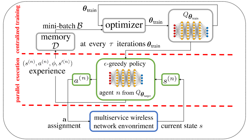
Figure 1: llustration of the proposed multi-agent deep RL algorithm for resource allocation [14], adapted.

After that, in line 10, we define an experience sample as a tuple, $(s^{(n)},a^{(n)},\phi,s^{\prime(n)})$, consisting in current state $s^{(n)}$, chosen action $a^{(n)}$, reward $\phi$ and next state, $s^{\prime(n)}$ of each agent. In addition, in order to avoid oscillations and divergence in the parameters, we use the concept of memory replay so that the tuples of experiences of all agents are stored in memory $\mathcal{D}$. We consider that this memory is a FIFO queue where a new experience replaces the oldest experience in the queue when the number of experiences exceeds the capacity, $D$. In order to train the parameters $\mbox{\boldmath{$\theta$}}_{\text{train}}$, a mini-batch of experiences, $\mathcal{B}$, is sampled randomly from $\mathcal{D}$ and the stochastic gradient descent method is performed by central module to minimize the cost function in (5) as shown in lines 11 and 12, respectively. Furthermore, the process of updating the parameters $\mbox{\boldmath{$\theta$}}_{\text{target}}$ is periodic and, therefore, in line 13, only at every $\tau$ episodes, the new parameters $\mbox{\boldmath{$\theta$}}_{\text{train}}$ are available for target DQN. Finally, in line 14, the $\epsilon$-greedy policy is updated, the current state of each agent changes to the next state (line 15) and another episode starts.

Mathematically, the complexity of Alg. 2 can be evaluated by quantifying the complexity to obtain the $Q$-function from the DQN and to train the weights of the DQN since this is the main idea of this algorithm. Obviously, it highly depends on the structure of the employed DQN and its parameters. As discussed, in our case, the DQN is composed by fully-connected layers and, thereby, the complexity of the algorithm is given by $\mathcal{O}(wm\log m)$ where $w$ is the number of layers and $m$ is the number of units per layer [22].

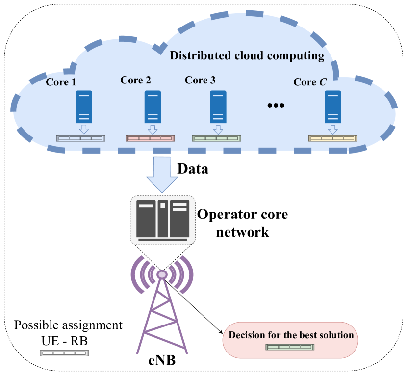
Figure 2: Proposed solution to problem (2) using parallel execution of Alg. 2 on different cores.

Something interesting about Alg. 2 is that depending on the initialization of the DQN weights or parameters, the algorithm can converge to a solution more or less accurately relative to the optimal solution of problem (2), given a fixed number of episodes. Indeed, this can be exploited by letting Alg. 2 run multiple times on different cores and, therefore, with totally independent weights initialization. As a result, since the runtime of each core is the same, the idea is to choose the best output as a solution to problem (2) as depicted in Fig. 2. Note that parallel execution of multiple cores does not necessarily need to be computed on the eNB itself. Due to possible limitations of this infrastructure such as overhead, small storage space and low computing ability, the data storage and processing can be moved to decentralized and powerful computing platforms located in a cloud. In terms of performance, the cloud utilizes distributed system architectures and can offer excellent computation speeds. Besides, cloud computing provides many other advantages as quick deployment, easy integration, resiliency, redundancy, backup, disaster recovery, among others [23]. Thus, the eNB is limited to deciding the best solution after data processing.

VI Performance Evaluation

In this section, we evaluate our proposed solution and compare it with the optimal solution and with the solutions of [1], [2] and [13]. We firstly present the main simulations parameters and, after that, the results and their discussion.

VI-A Simulation Assumptions

We consider 6 RB ($N=6$), 4 UE ($J=4$), 2 service plans ($L=2$) and we admit that UE from service plan $2$ demand a throughput of $150$ kbps higher than the UE from the service plan $1$. In both services, we consider only two UE, where $\eta_{1}=2$ and $\eta_{2}=1$. We assume $11$ QoS levels in kbps such that $\xi_{j\in\mathcal{J}_{1}}=(150,220,\dots,850)$, i.e., the required data rates for service plan $1$ vary between $150$ kbps and $850$ kbps at the step of $70$ kbps. Consequently, the requeriments for service plan $2$ vary between $300$ and $1000$ with the same step. The DQN was implemented using Tensorflow [24], assuming two hidden layers. We use the rectifier linear unit (ReLU) as DQN’s activation function and we use Adam’s algorithm [25] for the optimization. Moreover, we consider that $\epsilon$-greedy policy varies over the episodes following an exponential decay. In general, all the important simulation parameters are shown in Table I and Table II.

To perform qualitative comparisons with our proposed algorithm (deep $Q$-RA), we simulate the optimal solution of problem $\eqref{EQ:OBJ2}$ (OPT) as well as the algorithms Reallocation-based Assignment for Improved Spectral Efficiency and Satisfaction (RAISES) [1], Rate Maximization under Experience Constraints (RMEC) [2] and $Q$-learning based Resource Assignment ($Q$-RA) [13]. On one hand, RAISES and RMEC are traditional rule-based algorithms, which use resource reallocation strategies to define the best assignment pattern for the system. On the other hand, $Q$-RA, as its name suggests, is an algorithm based on $Q$-learning technique for resource allocation. Therefore, $Q$-RA algorithm is a tabular learning method, where a single agent accumulates all its experience in a $Q$-table over several episodes.

Regarding the performance metrics, we consider the outage rate and the system throughput. An outage event happens when an algorithm cannot manage to find a feasible solution, i.e., the algorithm does not find a solution fulfilling the constraints of problem (2). Then, outage rate is defined as the ratio between the number of instances with outage events and the total number of simulated instances. The system throughput is the sum of the data rates obtained by all the UE in a given instance. The results were obtained by running $1,000$ feasible instances of problem (2) in order to get valid results in a statistical sense and the channel realizations were the same for all the simulated algorithms to get fair comparisons.

TABLE I: DQN Parameters

Parameter	Value
Memory size	1000
Mini-batch size	256
Number of neurons per hidden layer	64
Initial value for $\epsilon$	0.8
Decay rate	0.001
Learning rate	0.0001
Discount factor	0
Period for updating target DQN weights	5

TABLE II: Network Parameters [1]

Parameter	Value
Cell radius	$334\text{\,}\mathrm{m}\text{/}$
Transmit power per RB	$0.35\text{\,}\mathrm{W}\text{/}$
Number of subcarriers per RB	12
Shadowing standard deviation	$8\text{\,}\mathrm{dB}\text{/}$
Path loss	35.3 + 37.6$\ \cdot\log(d)$ [$\text{\,}\mathrm{dB}\text{/}$]
Traffic model	Full buffer
Noise spectral density	3.16$\ \cdot 10^{-20}$ $\text{\,}\mathrm{W}\text{/}$/$\text{\,}\mathrm{Hz}\text{/}$

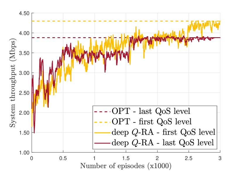
Figure 3: System throughput versus number of episodes in a particular instance for OPT and deep $Q$-RA algorithms.

VI-B Numerical Results

Fig. 3 shows the system throughput versus the number of episodes for the algorithms OPT and deep $Q$-RA, condesidering the first and the last QoS levels described in Section VI-A. Looking at the performance of the deep $Q$-RA solution, we can observe that it converges to the OPT solution as the number of episodes increases for both investigated QoS levels. This is an expected result since the more episodes we have, the more accurate the estimation of $Q$-function is and, consequently, the more favorable it is for the agents to converge to the optimal solution of problem (2). Moreover, note that in Fig. 3 the convergence time to the optimal solution may vary depending on the required QoS level. This is because at low QoS levels there are several possible solutions and, as a result, it can be more difficult to converge to the optimal solution of problem (2). For scenarios with high QoS levels required, possible solutions are rarer but once found means near optimal solutions, consequently the deep $Q$-RA algorithm tends to focus on them. Indeed, this can lead to faster convergence.

In Fig. 4 and Fig. 5, we plot the system throughput and outage rate versus the number of parallel cores in the system, respectively, in order to show the advantages of the structure illustrated in Fig. 2. Also, from here, we assume for all the following results a confidence interval with a $95\%$ confidence level. Firsty, in Fig. 4 and Fig. 5, note that as the number of cores in the system increases, there is a considerable increase in the performance of the proposed solution. In addition, due to the characteristics of the deep $Q$-learning technique, this structure does not require a high memory consumption and, as shown in the last figures, a relatively low number of cores is enough to ensure excellent performance. Note, for example, that with less than $10$ cores there is practically no outage in the system for the investigated scenario.

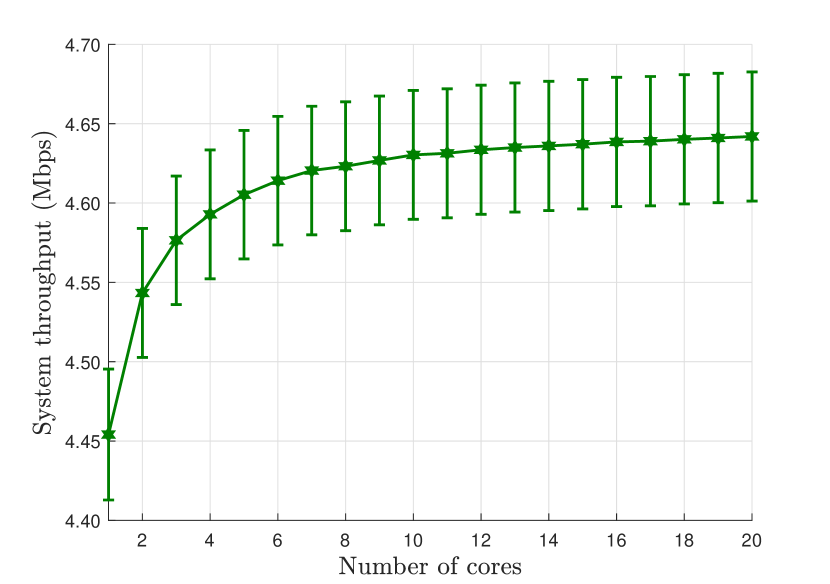
Figure 4: System throughput of deep $Q$-RA algorithm versus the number of parallel cores in the system.

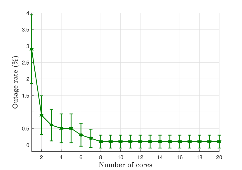
Figure 5: Outage rate of deep $Q$-RA algorithm versus the number of parallel cores in the system.

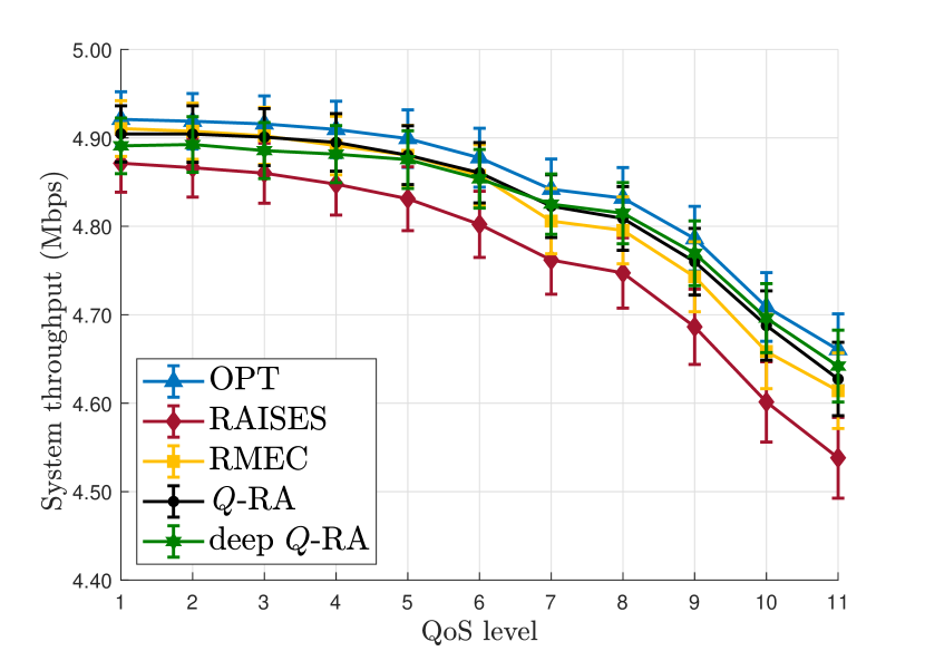
Figure 6: System throughput versus QoS level for OPT, RAISES, RMEC, $Q$-RA and deep $Q$-RA algorithms in the considered scenario.

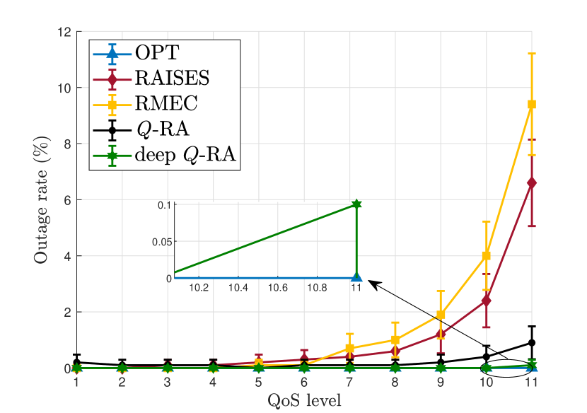
Figure 7: Outage rate versus QoS level for OPT, RAISES, RMEC, $Q$-RA and deep $Q$-RA algorithms in the considered scenario.

Now we compare our approach with other proposals from the literature. In Fig. 6 and Fig. 7, we plot the system throughput and the outage rate in the considered scenario versus the QoS level for the algorithms OPT, RAISES, RMEC, $Q$-RA and deep $Q$-RA, respectively. For the $Q$-RA and deep $Q$-RA algorithms, we consider $3,000$ episodes in the plots of these figures. Besides, for deep $Q$-RA algorithm we use $10$ cores. In this way, we firstly observe a near optimal performance of our proposed solution both in terms of outage rate and system throughput to problem (2). In fact, we highlight Fig. 7 that shows the outage curve that is considerably better for the solutions based on RL, with even better performance for deep $Q$-RA solution. In this figure, notice that the outage rate for these solutions are smaller than $1\%$ and $0.1\%$ for $Q$-RA and deep $Q$-RA, respectively.

On the other hand, RAISES and RMEC solutions have much higher outage rates, with approximately $7\%$ and $10\%$ for the highest QoS level, respectively. This shows that solutions based on ML algorithms may perform better than traditional heuristics and, therefore, they can be considered as a promising tool to solve resource allocation problems in modern networks. However, as highlighted in [13], $Q$-RA solution may require a high memory cost to build and store $Q$-table because it directly depends on space $\mathcal{S}\times\mathcal{A}$. Therefore, this makes its use more difficult in interesting and realistic scenarios. As discussed earlier, this is not a problem for deep $Q$-RA solution, which may in fact become a more attractive and less problematic solution in larger scenarios.

VII Conclusions and Perspectives

In this paper, we have investigated the problem of maximizing the system throughput subject to user satisfaction ratio constraints in a multiservice scenario. This problem was previously studied in [1], [2] and [13], where tradicional heuristics or machine learning based methods were proposed. However, to tackle this problem we have proposed a new decentralized radio resource allocation mechanism employing multi-agent deep reinforcement learning. From the simulation results, we have shown that each agent can learn how to jointly deal with resource allocation and QoS garantees while maximizing the system throughput. As a result, our proposed can provide better performance than the other benchmark approaches simulated in this article.

Regarding future works, we believe that the proposed framework in this paper can be improved by taking into consideration the channel correlation along the time and redefining the system state in order to considerably decrease the need for training when applied in dynamic contexts. Finally, other approaches where learning-based techniques are jointly responsible for allocating power and resource can also be analyzed in the future.

References

- [1] Francisco Rafael Marques Lima, Tarcisio Ferreira Maciel, Walter Cruz Freitas and Francisco Rodrigo Porto Cavalcanti “Resource assignment for rate maximization with QoS guarantees in multiservice wireless systems” In IEEE Transactions on Vehicular Technology 61.3, 2012, pp. 1318–1332 DOI: 10.1109/TVT.2012.2183905
- [2] Diego Aguiar Sousa et al. “Resource Management for Rate Maximization with QoE Provisioning in Wireless Networks” In Journal of Communication and Information Systems 31.1, 2016 DOI: 10.14209/jcis.2016.25
- [3] Victor Farias Monteiro et al. “Distributed RRM for 5G Multi-RAT Multiconnectivity Networks” In IEEE Systems Journal 13.1, 2019, pp. 192–203 DOI: 10.1109/JSYST.2018.2838335
- [4] Francesco Davide Calabrese et al. “Learning Radio Resource Management in RANs: Framework, Opportunities, and Challenges” In IEEE Communications Magazine 56.9, 2018, pp. 138–145 DOI: 10.1109/MCOM.2018.1701031
- [5] K.. Ahmed, H. Tabassum and E. Hossain “Deep Learning for Radio Resource Allocation in Multi-Cell Networks” In IEEE Network 33.6, 2019, pp. 188–195 DOI: 10.1109/MNET.2019.1900029
- [6] Eduardo Castaneda, Adao Silva, Atilio Gameiro and Marios Kountouris “An Overview on Resource Allocation Techniques for Multi-User MIMO Systems” In IEEE Communications Surveys and Tutorials 19.1, 2017, pp. 239–284 DOI: 10.1109/COMST.2016.2618870
- [7] Volodymyr Mnih et al. “Human-level control through deep reinforcement learning” In Nature 518.7540 Nature Publishing Group, 2015, pp. 529–533
- [8] Qian Mao, Fei Hu and Qi Hao and “Deep Learning for Intelligent Wireless Networks: A Comprehensive Survey” In IEEE Communications Surveys and Tutorials 20.4, 2018, pp. 2595–2621 DOI: 10.1109/COMST.2018.2846401
- [9] Y. Sun, M. Peng and S. Mao “Deep Reinforcement Learning-Based Mode Selection and Resource Management for Green Fog Radio Access Networks” In IEEE Internet of Things Journal 6.2, 2019, pp. 1960–1971 DOI: 10.1109/JIOT.2018.2871020
- [10] Roohollah Amiri and Hani Mehrpouyan “Self-Organizing mm Wave Networks: A Power Allocation Scheme Based on Machine Learning” In Proceedings of the Global Symposium on Millimeter Waves (GSMM), 2018, pp. 1–4 DOI: 10.1109/GSMM.2018.8439323
- [11] Richard S Sutton and Andrew G Barto “Reinforcement learning: An introduction” MIT press, 2018
- [12] Jordi Pérez-Romero et al. “Power-Efficient Resource Allocation in a Heterogeneous Network With Cellular and D2D Capabilities” In IEEE Transactions on Vehicular Technology 65.11, 2016, pp. 9272–9286 DOI: 10.1109/TVT.2016.2517700
- [13] Juno Vitorino Saraiva et al. “A Q-learning Based Approach to Spectral Efficiency Maximization in Multiservice Wireless Systems” In Proceedings of the Brazilian Telecommunications Symposium (SBrT), 2019
- [14] Yasar Sinan Nasir and Dongning Guo “Multi-Agent Deep Reinforcement Learning for Dynamic Power Allocation in Wireless Networks” In IEEE Journal on Selected Areas in Communications 37.10, 2019, pp. 2239–2250 DOI: 10.1109/JSAC.2019.2933973
- [15] H. Ye, G.. Li and B.. Juang “Deep Reinforcement Learning Based Resource Allocation for V2V Communications” In IEEE Transactions on Vehicular Technology 68.4, 2019, pp. 3163–3173
- [16] Nan Zhao et al. “Deep Reinforcement Learning for User Association and Resource Allocation in Heterogeneous Cellular Networks” In IEEE Transactions on Wireless Communications 18.11, 2019, pp. 5141–5152 DOI: 10.1109/TWC.2019.2933417
- [17] Ying He et al. “Software-Defined Networks with Mobile Edge Computing and Caching for Smart Cities: A Big Data Deep Reinforcement Learning Approach” In IEEE Communications Magazine 55.12, 2017, pp. 31–37 DOI: 10.1109/MCOM.2017.1700246
- [18] Y. He et al. “Deep-Reinforcement-Learning-Based Optimization for Cache-Enabled Opportunistic Interference Alignment Wireless Networks” In IEEE Transactions on Vehicular Technology 66.11, 2017, pp. 10433–10445 DOI: 10.1109/TVT.2017.2751641
- [19] Vincent François-Lavet et al. “An introduction to deep reinforcement learning” In Foundations and Trends® in Machine Learning 11.3-4 Now Publishers, Inc., 2018, pp. 219–354 DOI: 10.1561/2200000071
- [20] Zhuoran Yang, Yuchen Xie and Zhaoran Wang “A theoretical analysis of deep Q-learning” In arXiv preprint arXiv:1901.00137, 2019
- [21] Hado Hasselt, Arthur Guez and David Silver “Deep reinforcement learning with double Q-learning” In Thirtieth AAAI conference on artificial intelligence, 2016
- [22] Hyun-Suk Lee, Jin-Young Kim and Jang-Won Lee “Resource Allocation in Wireless Networks With Deep Reinforcement Learning: A Circumstance-Independent Approach” In IEEE Systems Journal, 2019, pp. 1–04 DOI: 10.1109/JSYST.2019.2933536
- [23] Ahmed Alzahrani, Nasser Alalwan and Mohamed Sarrab “Mobile Cloud Computing: Advantage, Disadvantage and Open Challenge” In Proceedings of the 7th Euro American Conference on Telematics and Information Systems New York, NY, USA: Association for Computing Machinery, 2014 DOI: 10.1145/2590651.2590670
- [24] Martı́n Abadi “TensorFlow: A System for Large-Scale Machine Learning” In Proc. USENIX Symposium on Operating Systems Design and Implementation, 2016, pp. 265–283
- [25] Diederik P. Kingma and Jimmy Ba “Adam: A Method for Stochastic Optimization” In CoRR abs/ 1412.6980, 2014 arXiv: https://arxiv.org/abs/1412.6980v9