Dimensionality Reduction of Movement Primitives in Parameter Space

Abstract

Movement primitives are an important policy class for real-world robotics. However, the high dimensionality of their parametrization makes the policy optimization expensive both in terms of samples and computation. Enabling an efficient representation of movement primitives facilitates the application of machine learning techniques such as reinforcement on robotics. Motions, especially in highly redundant kinematic structures, exhibit high correlation in the configuration space. For these reasons, prior work has mainly focused on the application of dimensionality reduction techniques in the configuration space. In this paper, we investigate the application of dimensionality reduction in the parameter space, identifying principal movements. The resulting approach is enriched with a probabilistic treatment of the parameters, inheriting all the properties of the Probabilistic Movement Primitives. We test the proposed technique both on a real robotic task and on a database of complex human movements. The empirical analysis shows that the dimensionality reduction in parameter space is more effective than in configuration space, as it enables the representation of the movements with a significant reduction of parameters.

I Introduction

Robot learning is a promising approach to enable more intelligent robotics, which can easily adapt to the user’s desires. In recent years, the field of reinforcement learning (RL) has experienced an enormous advance in solving simulated tasks such as board- or video-games [1, 2, 3], in contrast to little improvements in robotics. The major challenges in the direct application of RL to real robotics, are mainly the limited availability of samples and the fragility of the system, which disallow the application of unsafe policies. These two disadvantages become even more evident when we consider that usual robotic tasks such as industrial manipulation, are defined in a high dimensional state and action space. A usual approach in the application of RL to robotics, is to initialize the policy via imitation learning [4, 5, 6, 7]. In the past, there has been some effort in providing a safe representation of the policy for robotics, mainly by the means of Movement Primitives (MPs) [8, 9, 10, 11]. The general framework of MPs has been extensvely studied and employed in a large variety of settings [12, 13, 14, 15, 16].

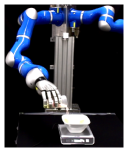
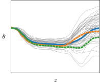
Figure 1: Our binamual platform performing a pouring task using Pro-Primos (left). The generation of trajectories via PriMos (right): the blue line corresponds to the mean movement, while the dashed lines to the principal movements. By only linearly combining two principal movements, it is possible to generate a wide variety of movements (gray lines).

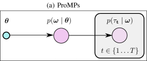
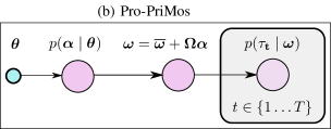
Figure 2: Graphical model of the ProMPs framework (a) compared to Pro-PriMos (b). The main idea of Pro-PriMos is to generate a distribution of linear combinations of the principal-movements $\bm{\Omega}$.

MPs have been shown to be effective when used for the direct application of RL to robotics [17, 18, 19]. The drawback of the general framework of MPs, is the usual high number of parameters. In fact, in the configuration-space, the number of parameters is equal to the number of basis functions (typically greater than 10), times the number of degree-of-freedom (DoF). The number of parameters grows even quadratically w.r.t. the number of basis function and DoF when we want to represent the full covariance matrix in the case of Probabilistic Movement Primitives (ProMPs) [11, 20]. In recent years, many authors have proposed techniques to solve the problem by using a latent representation of the robot’s kinematic structure [21, 22, 23, 24]. Especially for complex systems, such as humanoids, many DoF are redundant, and a compressed representation of the configuration-space results in a lighter parametrization of the MP. However, this approach is less effective in the case of a robotic arm with fewer DoF Moreover, the parametrization of the MPs would be still linear w.r.t. the number of basis functions.

In this article, we build on the general framework of ProMPs and we propose to apply the dimensionality reduction in parameter space. In tasks where there is a high correlation between the movements, it makes more sense to seek a compressed representation of the movement instead of the configuration-space. To this end, we propose an approach where the movements can be seen as a linear combination of principal movements (Fig.1). We enrich our framework with a probabilistic treatment of the parameters, so that our approach inherits all the properties of ProMPs. We analyze the benefit of dimensionality reduction in the parameter space w.r.t. in configuration space, both on a challenging human motion reconstruction and in a robotic pouring task (Fig. 1). Our findings show that our proposed approach achieve satisfying accuracy even with a significant reduction of parameters.

II Related Work

The issue of dimensionality reduction in the context of motor primitives has been extensively studied. To achieve dimensionality reduction for Dynamic Movement Primitives (DMPs) [9], the autoencoded dynamic movement primitives model proposed in [23], uses to find a representation of the movements in a latent feature space, while in [24] the DMPs are embedded into the latent space of a time-dependent variational autoencoder. In [22] a linear projection in the latent space of the configuration space is considered, as well as the adaption of the projection matrix in the RL context. Interestingly, they consider the possibility to address the dimensionality reduction in the parameter space, but they discard this option as the projection matrix is more difficult to adapt since it is of higher dimensions. We agree with this argument, however, when we assume that the projection matrix can be considered fixed this argument is not valid anymore. The dimensionality reduction of ProMPs has been addressed in [25], where the authors compare PCA versus an expectation-maximization approach in configuration space. Until this point, all the literature is focused in finding a mapping between configuration space and a latent space, and proposing the learning of the MPs in this lower representation. However, this approach results to be more efficient in complex kinematic structures, such as the human body, where the high number of joints facilitate the possibility of redundancies in the configuration space. Moreover, this reduction, does not affect the intrinsic high-dimensional nature of the MPs, which requires usually a high number of basis functions.

A way to overcome this problem is to focus in the parameter space of the movement primitives. The dimensionality reduction in this case exploits similarities between movements, and high correlations between parameters. To the best of our knowledge, the only work performing a reduction in parameter is [26]. The proposed setup is however complex as it considers a fully hierarchical Bayesian setting, where the movements are encoded by a mixture of Gaussian models. They learn those parameters using variational inference. Furthermore, their approach does not address the question of whether the parameter space reduction is more convenient or not.

In our paper, we want to focus on the comparison between the dimensionality reduction in configuration and parameter space, arguing that the latter is more convenient. To this end, we propose the Principal Movements (PriMos) framework, which enables the selection of principal movements and the subsequent representation of the movements in this convenient space. We extend PriMos to incorporate a probabilistic treatment of the parameters (Pro-PriMos), in a similar way to the ProMPs framework. Our approach only adds a linear transformation to the framework already developed by Parachos et al., as depicted in Fig. 2, therefore it maintains all the properties exposed by the ProMPs, such as time modulation, movements co-activation or movement conditioning. To maintain the method simple, we select PCA for the dimensionality reduction, even if more sophisticated techniques can be used.

III The Principal Movement Framework

Machine learning, should allow the robotic agent to interact with the real world in a non-predetermined way. However, the possible generated movement should be smooth, and possibly constrained to be safe (not colliding with other objects, without excessive speed or accelerations, etc). These issues require a whole field of research to be solved. MPs are useful in this context. The idea behind MPs, is to restrict the class of all possible robotic movements to a specific parameterized class usually by linearly combining a set of parameters with a set of features. For a particular class of features (e.g., radial basis function), the movements are guaranteed to be smooth. However, sometimes restricting the space of robotic movement to be smooth is not enough, and we want also the movements to be distributed similarly to some demonstration provided by a human expert. The ProMPs provides a probabilistic treatment of the movement’s parameters [11, 20]. Both frameworks are useful and can be coupled with RL. In the following, we introduce the Principal Movements (PriMos) framework, as well as its probabilistic extension (Pro-PriMos). In Section III-A, we introduce the formal notation of the MPs framework. In Sections III-B and III-C, we introduce PriMos and Pro-PriMos relying on the assumption that a set of principal movement is given. In Section III-D we propose a technique to find the principal movements, offering a complete algorithm for dimensionality reduction for MPs.

III-A Preliminaries

Let us concisely introduce the notation and formalize the classic MPs framework. For simplicity, we will first consider only a one-dimensional trajectory $\bm{\tau}^{\intercal}=[\tau_{1},\dots,\tau_{T}]$, where $\tau_{i}$ represent the joint’s position at time $t_{i}$. In order to introduce the time modulation, we use a phase-vector z where $z_{i}=(t_{i}-t_{1})/(t_{T}-t_{1})$. Moreover, we consider $n$ normalized radial-basis functions $\Phi_{i}:\mathbb{R}\to\mathbb{R}$, usually, ordered to evenly cover the phase-space, they are centered between $[-2h,1+2h]$ where $h$ is the bandwidth. At time $t$ the features are described by a $n$-dimensional column vector $\bm{\Phi}_{t}$ where $\Phi_{t,i}=\Phi_{i}(z_{t})$. Assuming that the observations are perturbed by a zero-mean Gaussian noise $\epsilon_{t}$ with variance $\sigma_{\tau}$, we want to represent the movement $\tau_{t}=\bm{\Phi}_{t}^{\intercal}\bm{\omega}+\epsilon_{t}$ as a linear combination of parameters $\bm{\omega}\in\mathbb{R}^{n}$. , we obtain the following maximum-likelihood estimation (MLE) problem

$$\max_{\omega}\mathcal{L}(\bm{\omega})=\max_{\omega}\prod_{t}\mathcal{N}(\tau_{t}\mid\bm{\Phi}_{t}^{\intercal}\omega,\sigma_{t}).$$ (1)

Equation (1) can be solved with usual linear regression, or more commonly with Ridge-regression (which corresponds to have a prior Gaussian distribution on $\omega$, $\mathcal{N}(\omega_{i}|0;\sigma_{\omega})$) that leads to better generalization and is more numerically stable,

$$\bm{\omega}=\left(\bm{\Phi}^{\intercal}\bm{\Phi}+\lambda\mathbb{I}\right)^{-1}\bm{\Phi}^{\intercal}\bm{\tau}$$ (2)

where $\lambda$ is the ridge penalization term and $\bm{\Phi}^{\intercal}=[\bm{\Phi}_{1},\bm{\Phi}_{2}\dots,\bm{\Phi}_{T}]$. However, there is the possibility to extend this setting with a probabilistic treatment of the movement parameters. In this case, we want to find the best distribution over parameters which encode a distribution of trajectories, i.e.,

$$p(\bm{\tau}\mid\mu_{\omega},\Sigma_{\omega})=\int p(\bm{\tau}\mid\omega)\mathcal{N}(\bm{\omega}\mid\mu_{\omega};\Sigma_{\omega})\mathrm{d}\bm{\omega}.$$ (3)

This is the setting described with ProMPs in [11]. For a finite set of stroke-movements $\{\bm{\tau}_{i}\}_{i=1}^{m}$, it is possible to use the parameters $\bm{\omega}_{i}$ estimated for each trajectory $\bm{\tau}_{i}$ in order to estimate $\bm{\mu}_{\omega}$ and $\bm{\Sigma}_{\omega}$, i.e.,

$$\bm{\mu}_{\omega}=\frac{1}{m}\sum_{i=1}^{m}\bm{\omega}_{i},\quad\bm{\Sigma}_{\omega}=\frac{1}{m}\sum_{i=1}^{m}(\bm{\omega}_{i}-\bm{\mu}_{\omega})(\bm{\omega}_{i}-\bm{\mu}_{\omega})^{\intercal}.$$ (4)

In a more realistic scenario, we need to represent multiple joints. Assuming a system with $d$ joints, we can encode $\bm{\tau}^{\intercal}=[\tau_{1,1},\dots,\tau_{1,T},\dots,{\tau_{d,T}}]$ where $\tau_{i,j}$ is the position of the $i^{\text{th}}$ joint at time $t_{j}$, $\bm{\Psi}=\mathbb{I}\otimes\bm{\Phi}$ (where $\mathbb{I}$ is the $d\times d$ identity matrix) and $\bm{\omega}$ column-vector of length $nd$ encoding the movement’s parameters. Similarly to the notation already used, we denote with $\bm{\Psi}_{t}$ the feature matrix corresponding to the time step $t$.

III-B Principal Movements

The MPs and ProMPs frameworks, usually require a large number of parameters for encoding the movements. In MPs, we need in fact $d\times n$ parameters (where $d$ is the dimension of the considered movement and $n$ is the number of radial basis functions). rThe choice of the number of radial-basis functions usually depends by both the speed and the complexity of the movements, but most of the time it is greater than ten. For a $7$ d.o.f. we, therefore, need at least $70$ parameters to encode the MPs. This makes the application of RL challenging for a 7 d.o.f. robot arm. We will assume, from now on, that an oracle (i.e., a human expert or a dimensionality reduction method) will give us the parameters of a mean-movement $\overline{\bm{\omega}}$, and a matrix of principal-movements $\bm{\Omega}^{\intercal}=[\bm{\omega}^{p}_{1},\dots,\bm{\omega}^{p}_{n_{c}}]$. We therefore want to encode a given trajectory $\bm{\tau}$ as a linear combination of the principal movements, i.e.,

$$\bm{\tau}_{t}=\bm{\Psi}_{t}\overline{\bm{\omega}}+\bm{\Psi}_{t}\bm{\Omega}\bm{\alpha}+\epsilon_{t}.$$ (5)

We consider $\bm{\alpha}\in\mathbb{R}^{n_{c}}$ the new parameter vector. Note that $n_{c}$ is generally independent of the number of joints $d$ and of the number of radial basis function $n$, but instead the choice of $n_{c}$ is connected to the complexity of the movement-space that we aim to represent. The MLE problem

$$\max_{\bm{\alpha}}\prod_{t}\mathcal{N}(\bm{\tau}_{t}\mid\bm{\Psi}_{t}\overline{\bm{\omega}}+\bm{\Psi}_{t}\bm{\Omega}\bm{\alpha},\sigma_{t}),$$ (6)

induced by (5) has a Ridge regression solution

$$\bm{\alpha}=\left(\bm{\Omega}^{\intercal}\bm{\Psi}^{\intercal}\bm{\Psi}\bm{\Omega}+\lambda\mathbb{I}\right)^{-1}\bm{\Omega}^{\intercal}\bm{\Psi}^{\intercal}\left(\bm{\tau}-\bm{\Psi}\overline{\bm{\omega}}\right).$$ (7)

III-C Probabilistic Principal Movements

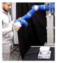
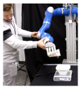
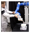
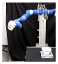
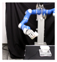
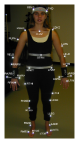
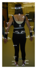
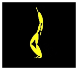
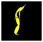
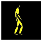
Figure 3: Top: From left to right, the demonstration in kinestatic teaching mode of the pouring task, and the subsequent reconstruction of the movement with PriMos. Bottom: Markers placements on the human body, and illustrative example of the skeleton reconstruction for a “walk and pick-up” task of subject #143 of the MoCap database http://mocap.cs.cmu.edu.

A probabilistic treatments of the MPs, is often convenient, as it enables the application of statistical tools [11, 20]. To enrich our approach with a probabilistic treatment, we assume our parameter vector $\bm{\alpha}$ to be multivariate-Gaussian distributed, i.e., $\bm{\alpha}\sim\mathcal{N}(\cdot\mid\bm{\mu}_{\alpha};\bm{\Sigma}_{\alpha})$. Very similarly to the classic ProMPs approach, we have that

$$p(\bm{\tau}_{t}\mid\bm{\mu}_{\alpha},\bm{\Sigma}_{\alpha})$$

$$= \int\mathcal{N}(\bm{\tau}_{t}\mid\bm{\Psi}_{t}(\bm{\Omega}\bm{\alpha}+\overline{\bm{\omega}}),\bm{\Sigma}_{\tau})\mathcal{N}(\bm{\alpha}\mid\bm{\mu}_{\alpha},\bm{\Sigma}_{\alpha})\mathrm{d}\bm{\alpha}$$

$$= \mathcal{N}(\bm{\tau}_{t}\mid\bm{\Psi}_{t}(\bm{\Omega}\bm{\mu}_{\alpha}+\overline{\bm{\omega}}),\bm{\Psi}_{t}\bm{\Omega}\bm{\Sigma}_{\alpha}\bm{\Omega}^{\intercal}\bm{\Psi}_{t}^{\intercal}+\bm{\Sigma}_{\tau}).$$ (8)

The mean $\bm{\mu}_{\alpha}$ and the covariance $\bm{\Sigma}_{\alpha}$ can be estimated as similarly done for ProMPs, (Eq. 4)

$$\bm{\mu}_{\alpha}=\frac{1}{m}\sum_{i=1}^{m}\bm{\alpha}_{i},\quad\bm{\Sigma}_{\alpha}=\frac{1}{m}\sum_{i=1}^{m}(\bm{\alpha}_{i}-\bm{\mu}_{\alpha})(\bm{\alpha}_{i}-\bm{\mu}_{\alpha})^{\intercal},$$ (9)

where the parameters $\bm{\alpha}_{i}$ correspond to the trajectories $\bm{\tau}_{i}$.

We assume an affine transformation between the full parameters $\bm{\omega}$ and the reduced $\bm{\alpha}$, as shown in Fig. 2, and $\bm{\alpha}$ is assumed to be Gaussian distributed. Under these assuptions, $\bm{\omega}$ is also Gaussian distributed, allowing for a mapping from Pro-PriMos to ProMPs,

$$\hat{\bm{\mu}}_{\omega}=\bm{\Omega}\bm{\mu}_{\alpha}+\overline{\bm{\omega}},\quad\quad\hat{\bm{\Sigma}}_{\omega}=\bm{\Omega}\bm{\Sigma}_{\alpha}\bm{\Omega}^{\intercal}.$$

Hence, the proposed framework enjoys all the properties of the ProMPs, such as movements co-activation or movement conditioning.

III-D Inference of the Principal Components

Until this point, we considered the parameters $\overline{\bm{\omega}}$ and $\bm{\Omega}$ given by an oracle. We mentioned that the underlying assumption of our work is that each movement can be seen as a linear combination of some movements which we call principal movements. To be precise, we assume that every trajectory $\bm{\tau}$ can be seen as $\bm{\tau}=\overline{\bm{\tau}}+\sum_{i}\bm{\tau}^{p}_{i}\alpha_{i}$. Since there exists a linear combination between the trajectory $\bm{\tau}$ and its parameter $\bm{\omega}$, we can argue, that the same relation exists in the parameter space. Reasoning in the parameter space is more convenient since the trajectories can have different lengths, depending on the sampling frequency and duration. The parameter space is instead fixed. We can say that the parameter space is frequency and duration agnostic. There are many techniques that can be used to estimate $\overline{\bm{\omega}}$ and $\bm{\Omega}$ when they are unknown, but among these, given the Gaussian assumption very made and also thanks to its simplicity, the Principal Component Analysis (PCA) [27] seems to be the most suited. We can think of the movement being Gaussian distributed with a certain mean trajectory $\overline{\bm{\tau}}$ (with parameters $\overline{\bm{\omega}}$) and with some orientation. In its geometric interpretation, the PCA extracts the main axis of the covariance matrix (i.e. the Eigenvectors of the covariance), and we can express each point in the new space as a linear combination of the Eigenvectors. Even though the Singular Value Decomposition is a more efficient technique to perform the PCA [28], we continue with the Eigenvector decomposition to maintain this parallelism. Let $\{\mathbf{v}_{i}\}_{i=1}^{nd}$ be the Eigenvectors of $\bm{\Sigma}_{\omega}$ and $\lambda_{i}$ the corresponding Eigenvalues (with $|\alpha_{1}|\geq|\alpha_{2}|\geq\dots$). To compute the projection matrix $\bm{\Omega}$ we select the first most informative $n_{c}$ Eigenvectors and we multiply them by the square roots of their corresponding Eigenvalues

$$\bm{\Omega}=\left[\bm{v}_{1}\sqrt{|\lambda_{1}|},\bm{v}_{2}\sqrt{|\lambda_{2}|},\dots,\bm{v}_{n_{c}}\sqrt{|\lambda_{n_{c}}|}\right].$$ (10)

This re-scaling gives us the possibility to have the principal movements scaled according to the variance of the data, and results in standardized values of $\bm{\alpha}$ (i.e. $\bm{\alpha}\sim\mathcal{N}(\cdot\sim\bm{0},\mathbb{I})$). Pro-PriMos is concisely summarized in Algorithm 1.

Algorithm 1 Pro-PriMos

A dataset of trajectories $\{\mathbf{z}_{i},\bm{\tau}_{i}\}_{i=1}^{m}$

for each $\mathbf{z}_{i},\bm{\tau}_{i}$ do

     Compute $\bm{\omega}_{i}$ with (2)

end for

Estimate $\bm{\mu}_{\omega}$ and $\bm{\Sigma}_{\omega}$ with (4)

Compute $\bm{\Omega}$ with (10)

Set $\overline{\bm{\omega}}:=\bm{\mu}_{\omega}$

for each $\mathbf{z}_{i},\bm{\tau}_{i}$ do

     Compute $\bm{\alpha}_{i}$ with (7)

end for

return $\bm{\mu}_{\alpha}\!=\!\frac{\sum_{i}\bm{\alpha}_{i}}{n_{c}}$; $\bm{\Sigma}_{\alpha}\!=\frac{\!\sum_{i}(\bm{\alpha}_{i}-\bm{\mu}_{\alpha})(\bm{\alpha}_{i}-\bm{\mu}_{\alpha})^{\intercal}}{n_{c}}$

IV Empirical Analysis

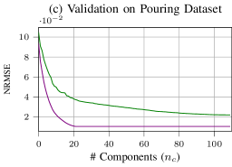
Figure 4: The number of parameters (y-axis) needed to achieve a certain accuracy (x-axis) (a), (b). As can be seen PriMos achieve better results with less samples. The error has been normalized in order to highlight the difference in complexity between the two datasets. In plot (b), both PriMo and CPCA fail in reaching a NRMSE lower than $0.08$. This is due to the complexity of the movement in the dataset, and by the maximum number of radial basis functions (20). In plots (c) we observe the comparison between train (blue) and validation error (green) achieved by PriMos in the pouring datasets.

We want to compare the dimensionality reduction in parameter space w.r.t. in configuration space. Therefore, we test the two approaches on two different scenario: the reconstruction of highly uncorrelated movements of a human subject, and on a dataset of pouring movements shown with a 7 DoF robotic arm. We also perform a qualitative analysis showing how our proposed method can achieve similar results to standard techniques, dramatically reducing the number of parameters.

The Human Motion Dataset

We want to apply PriMos to reconstruct some human motions contained in the MoCap dataset. The MoCap database contains a wide range of human motions (such as running, walking, picking up boxes, and even dancing) using different subjects (Fig. 3). Human motion is tracked using 41 markers with a Vicon optical tracking system. The data is preprocessed using Vicon Bodybuilder in order to reconstruct a schematic representation of the human body and the relative joint’s angles including the system 3D system reference, for a total of 62 values. The human motion is known to be highly redundant (i.e. many configurations are highly correlated), and therefore this is in principle the best case for the dimensionality-reduction in the configuration-space. The presence of many different typologies of movements, makes the application of PriMos challenging since our algorithm relies on the correlation between movements. In our experiments, we use the 42 movements recorded for the subject #143.

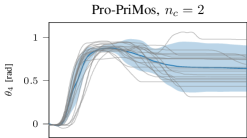
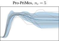
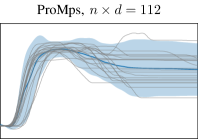
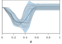
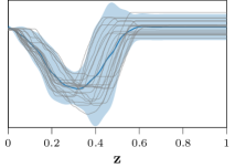
Figure 5: Mean movement of the joints most involved in the movements (shoulder and elbow), accompanied by the standard deviation ($\pm 2\sigma$) for Pro-PriMos with 2 and 5 components, and with ProMPs with 112 parameters for the mean. Note that the covariance matrix is encoded with 4, 25 and 12544 values respectively.

The Pouring Task

In the pouring task, we use a KUKA light-weight robotic arm with 7 DoF accompanied with a DLR-hand as an end-effector to pour some “liquid” (which, for safety reasons, is replaced by granular sugar). We record some motions from a human demonstrator, pouring some sugar in a bowl. The motion is recorded setting the robotic arm in kinestatic teaching. The quantity of sugar contained in the bowl is recorded by a DYMO digital scale with a sensitivity of $2g$. We aim to reconstruct the movements and understand whether our method is able to pour a similar amount of sugar: this experiment gives us a qualitative understanding, beyond the numerical accuracy analysis, to investigate the effectiveness of our algorithm in a real robot-learning task.

IV-A Accuracy of Movement Reconstruction

We want to compare the quality of the reconstruction using PriMos, and the dimensionality reduction in the configuration space. In order to be fair, we use PCA as reduction technique for both methods. In the remainder of the paper, we refer to the dimensionality reduction in the configuration space with the acronym “CPCA”.

Parameters vs Error Analysis

In this experiment, we want to assess the number of parameters needed to obtain a certain accuracy in the reconstruction. We, therefore, apply PriMos and CPCA to both the MoCap dataset and a dataset containing 15 different pouring movements. The CPCA admits several configurations for a fixed number of parameters (e.g., $100$ parameters can be obtained using $2$ components of the PCA and $50$ features or $4$ components and $25$ features, and so on). Therefore we created a grid of configuration in order to obtain the minimal amount of parameters to assess a certain accuracy. In order to make the results comparable between the MoCap and the pouring datasets, we use the normalized root mean square error (NRMSE) where the normalization is achieved dividing the RMSE by the standard deviation of the dataset. Fig. 4 depicts the NRMSE of PriMos and CPCA for the MoCap and pouring datasets. In both cases, the reduction in parameter space performed by PriMos requires significantly fewer parameter than the one performed in joint space by CPCA. Notably, for the MoCap database, the maximum number of basis functions chosen is not sufficient to achieve less than the $0.08$ reconstruction error.

Leave-One-Out Analysis

One might argue that our method “memorizes” the movements contained in the datasets. We want therefore to inspect the ability of PriMos to reconstruct movements not contained in the dataset (in other words, we want to understand if our method generalizes). We achieve this analysis using an increasing number of parameters and plotting the NRMSE using a leave-one-out strategy in the pouring dataset (we train on all the possible $n$ subsets of $n-1$ movements, and we test on the movement left out). More precisely, we fit $\overline{\bm{\omega}}$ and $\bm{\Omega}$ using the training set and then we test the error in the validation set. Fig. 4 shows that the error in the validation sets is not significantly higher than the training-error. Interestingly, while the training error becomes almost constant after $20$ components, the validation error keeps getting lower. This behavior suggests that our approach is robust against overfitting.

IV-B A Qualitative Evaluation

We want to understand the applicability of PriMos to real robotics. The study of the accuracy conducted is important, but on its own, it does not give us a feeling about how the method works in practice. For this reason, we use the 15 trajectories contained in the pouring dataset, and we measured the quantity of sugar poured in the bowl.

Single Movement Reconstruction

We run all the 15 trajectories reconstructed with the classic MPs and with PriMos for three times in order to average the stochasticity inherent to the experiment (a slight perturbation of the glass position or of the sugar contained in the glass might perturb the resulting quantity of sugar poured). A video of the demonstration as well of the reconstruction is available as supplementary material. Fig. 6 represents a confusion scatter plot: on the $x$-axis we have the weight of the sugar observed during the demonstration, while on the $y$-axis we observe the reconstructed movement both with MPs (112 parameters) and with PriMos (5 parameters). The ideal situation is when the points lye down on the identity line shown in green (perfect reconstruction). We observe that PriMos, except few outliers, reaches a similar accuracy to the MPs, but with $4.5\%$ of the parameters.

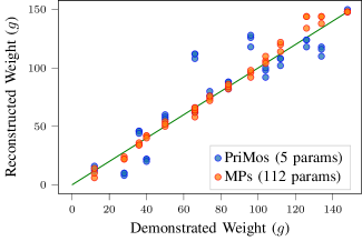
Figure 6: Precision of the reconstructed weight. The diagonal line represents the best possible reconstruction. For each demonstration, we repeated three times the reconstructed movement in order.

Probabilistic Representation

An important aspect of our framework is the possibility to represent the distribution of movements. For this reason, we show novel movements generated both with ProMPs and Pro-PriMos given $25$ demonstrations. The approximation of the full covariance-matrix is usually demanding, as it scales quadratically w.r.t. the number of parameters encoding the mean movement. Fig. 5 depicts the standard deviation of the shoulder of the robotic arm, within the demonstrated movement; Pro-PriMos seems to represent the stochasticity very similarly to the ProMPs, although the covariance matrix in the first case requires $5\times 5$ values, in contrast to $112\times 112$ required by the ProMPs. We also note that the variability of the Pro-PriMos seems to be lower than the ProMPs’ one: this behavior is explained by the fact that for a fixed set of features, PriMos represents a subset of movements of ProMPs. We furthermore sample 40 movements both from ProMPs and Pro-PriMos with $n_{c}=5$, and we measure the quantity of sugar poured. Table I shows that both the methods are able to pour all ranges of sugar (even if with different proportion from the demonstrated data). However, ProMPs occasionally fails to generate a good movement, and it pours the sugar outside the bowl. The video in the Supplementary Materials shows this situation.

Method	0-40$g$	40-80$g$	80-120$g$	120-150$g$	Failure
Demonstrations	20%	33%	27%	20%	0%
ProMPs	43%	7%	20%	17%	13%
Pro-PriMos	53%	20%	3%	24%	0

TABLE I: Measurement of sugar poured from 40 movements sampled both from ProMPs and Pro-PriMos. The methods manage to roughly resemble the original distribution, however ProMPs exhibit unwanted behaviors, like pouring most of the sugar outside the bowl (classified as “failures”).

V Conclusion

The main contribution of this paper is the analysis of the dimensionality reduction in parameter space in the context of MPs. Our findings suggest that this reduction is more efficient than the one in the configuration space. The novel approach (PriMos), which operates dimensionality reduction in the parameter space using the principal component analysis, is enriched with a probabilistic treatment of the parameters in order to inherit all the convenient properties of the ProMPs. We tested our approach both on a robotic task as well as in a challenging dataset of human movements. Our method compares well against the dimensionality reduction in configuration space, and exhibits a significant reduction of parameters with a modest loss of accuracy, even in the probabilistic setting. We argue that these insights are helpful to develop more efficient robot learning techniques.

As future work, we will investigate the application of different dimensionality reduction techniques in parameter space, with a special focus in the RL context.

References

- [1] V. Mnih, K. Kavukcuoglu, D. Silver, A. A. Rusu, J. Veness, M. G. Bellemare, A. Graves, M. Riedmiller, A. K. Fidjeland, G. Ostrovski, S. Petersen, C. Beattie, A. Sadik, I. Antonoglou, H. King, D. Kumaran, D. Wierstra, S. Legg, and D. Hassabis, “Human-Level Control Through Deep Reinforcement Learning,” Nature, vol. 518, no. 7540, pp. 529–533, 2015. [Online]. Available: http://www.nature.com/articles/nature14236
- [2] T. P. Lillicrap, J. J. Hunt, A. Pritzel, N. Heess, T. Erez, Y. Tassa, D. Silver, and D. Wierstra, “Continuous Control with Deep Reinforcement Learning,” in International Conference on Learning Representations, 2016, arXiv: 1509.02971. [Online]. Available: http://arxiv.org/abs/1509.02971
- [3] J. Schulman, F. Wolski, P. Dhariwal, A. Radford, and O. Klimov, “Proximal Policy Optimization Algorithms,” arXiv preprint arXiv:1707.06347, 2017.
- [4] S. Schaal, “Is Imitation Learning the Route to Humanoid Robots?” Trends in cognitive sciences, vol. 3, no. 6, pp. 233–242, 1999.
- [5] A. Billard and R. Siegwart, “Robot Learning from Demonstration,” Robotics and Autonomous Systems, vol. 2, no. 47, pp. 65–67, 2004.
- [6] B. D. Argall, S. Chernova, M. Veloso, and B. Browning, “A Survey of Robot Learning from Demonstration,” Robotics and autonomous systems, vol. 57, no. 5, pp. 469–483, 2009.
- [7] M. Rana, M. Mukadam, S. R. Ahmadzadeh, S. Chernova, and B. Boots, “Towards Robust Skill Generalization: Unifying Learning from Demonstration and Motion Planning,” in Intelligent robots and systems, 2018.
- [8] A. D’Avella, P. Saltiel, and E. Bizzi, “Combinations of Muscle Synergies in the Construction of a Natural Motor Behavior,” Nature Neuroscience, vol. 6, no. 3, pp. 300–308, 2003.
- [9] S. Schaal, J. Peters, J. Nakanishi, and A. Ijspeert, “Learning Movement Primitives,” in Robotics research. The eleventh international symposium. Springer, 2005, pp. 561–572.
- [10] S. M. Khansari-Zadeh and A. Billard, “Learning Stable Nonlinear Dynamical Systems with Gaussian Mixture Models,” IEEE Transactions on Robotics, vol. 27, no. 5, pp. 943–957, 2011.
- [11] A. Paraschos, C. Daniel, J. Peters, and G. Neumann, “Probabilistic Movement Primitives,” in Advances in Neural Information Processing Systems (NIPS). mit press, 2013.
- [12] H. B. Amor, G. Neumann, S. Kamthe, O. Kroemer, and J. Peters, “Interaction Primitives for Human-Robot Cooperation Tasks,” in IEEE international conference on robotics and automation (ICRA). IEEE, 2014, pp. 2831–2837.
- [13] G. Maeda, M. Ewerton, R. Lioutikov, H. B. Amor, J. Peters, and G. Neumann, “Learning Interaction for Collaborative Tasks with Probabilistic Movement Primitives,” in IEEE-RAS International Conference on Humanoid Robots. IEEE, 2014, pp. 527–534.
- [14] D. Koert, G. Maeda, R. Lioutikov, G. Neumann, and J. Peters, “Demonstration Based Trajectory Optimization for Generalizable Robot Motions,” in IEEE-RAS 16th International Conference on Humanoid Robots (Humanoids). IEEE, 2016, pp. 515–522.
- [15] G. Maeda, M. Ewerton, T. Osa, B. Busch, and J. Peters, “Active Incremental Learning of Robot Movement Primitives,” 2017.
- [16] S. Stark, J. Peters, and E. Rueckert, “Experience Reuse with Probabilistic Movement Primitives,” arXiv preprint arXiv:1908.03936, 2019.
- [17] J. Peters and S. Schaal, “Reinforcement Learning of Motor Skills with Policy Gradients,” Neural networks, vol. 21, no. 4, pp. 682–697, 2008.
- [18] J. Kober and J. R. Peters, “Policy Search for Motor Primitives in Robotics,” in Advances in Neural Information Processing Systems, 2009, pp. 849–856.
- [19] K. Mülling, J. Kober, O. Kroemer, and J. Peters, “Learning to Select and Generalize Striking Movements in Robot Table Tennis,” The International Journal of Robotics Research, vol. 32, no. 3, pp. 263–279, 2013.
- [20] A. Paraschos, C. Daniel, J. Peters, and G. Neumann, “Using Probabilistic Movement Primitives in Robotics,” Autonomous Robots (AURO), no. 3, pp. 529–551, 2018.
- [21] A. Colomé and C. Torras, “Dimensionality Reduction and Motion Coordination in Learning Trajectories with Dynamic Movement Primitives,” in IEEE/RSJ International Conference on Intelligent Robots and Systems. IEEE, 2014, pp. 1414–1420.
- [22] A. Colomé, G. Neumann, J. Peters, and C. Torras, “Dimensionality Reduction for Probabilistic Movement Primitives,” in International Conference on Humanoid Robots. IEEE, 2014, pp. 794–800.
- [23] N. Chen, J. Bayer, S. Urban, and P. Van Der Smagt, “Efficient Movement Representation by Embedding Dynamic Movement Primitives in Deep Autoencoders,” in IEEE-RAS 15th International Conference on Humanoid Robots (Humanoids). IEEE, 2015, pp. 434–440.
- [24] N. Chen, M. Karl, and P. Van Der Smagt, “Dynamic Movement Primitives in Latent Space of Time-Dependent Variational Autoencoders,” in 2016 IEEE-RAS 16th International Conference on Humanoid Robots (Humanoids). IEEE, 2016, pp. 629–636.
- [25] A. Colomé and C. Torras, “Dimensionality Reduction for Dynamic Movement Primitives and Application to Bimanual Manipulation of Clothes,” IEEE Transactions on Robotics, vol. 34, no. 3, pp. 602–615, 2018.
- [26] E. Rueckert, J. Mundo, A. Paraschos, J. Peters, and G. Neumann, “Extracting Low-Dimensional Control Variables for Movement Primitives,” in 2015 IEEE International Conference on Robotics and Automation (ICRA). IEEE, 2015, pp. 1511–1518.
- [27] K. Pearson, “On Lines and Planes of Closest fit to Systems of Points in Space,” The London, Edinburgh, and Dublin Philosophical Magazine and Journal of Science, vol. 2, no. 11, pp. 559–572, 1901.
- [28] G. H. Golub and C. F. Van Loan, Matrix Computations, 3rd ed. JHU press, 2012.