Seeding Approach to nucleation in the NVT ensemble: the case of bubble cavitation in overstretched Lennard Jones fluids

Abstract

Simulations are widely used to study nucleation in first order phase transitions due to the fact that they have access to the relevant length and time scales. However, simulations face the problem that nucleation is an activated process. Therefore, rare event simulation techniques are needed to promote the formation of the critical nucleus. The Seeding method, where the simulations are started with the nucleus already formed, has proven quite useful in efficiently providing estimates of the nucleation rate for a wide range of orders of magnitude. So far, Seeding has been employed in the NPT ensemble, where the nucleus either grows or redissolves. Thus, several trajectories have to be run in order to find the thermodynamic conditions that make the seeded nucleus critical. Moreover, the nucleus lifetime is short and the statistics for obtaining its properties is consequently poor. To deal with these shortcomings we extend the Seeding method to the NVT ensemble. We focus on the problem of bubble nucleation in a mestastable Lennard Jones fluid. We show that, in the NVT ensemble, it is possible to equilibrate and stabilise critical bubbles for a long time. The nucleation rate inferred from NVT-Seeding is fully consistent with that coming from NPT-Seeding. The former is quite suitable to obtain the nucleation rate along isotherms, whereas the latter is preferable if the dependence of the rate with temperature at constant pressure is required. Care should be taken with finite size effects when using NVT-Seeding. Further work is required to extend NVT seeding to other sorts of phase transitions.

I Introduction

The study of the onset of first order phase transitions by means of computer simulations has received a great deal of attention JCP_1992_96_04655 ; searJPCM2007 ; anwarAnge2011 ; reviewMichaelides2016 ; coluzza2017perspectives . Simulations is a very suited tool to study this phenomenon given that the nucleation of the stable phase in the parent mestastable phase typically entails hundreds of molecules and takes a few nanoseconds kelton . These are time and length scales accessible to simulations but difficult to probe in experiments.

One of the main difficulties that simulations face in nucleation studies is the activated nature of such process. As a consequence, there is a huge timescale difference between the duration of the nucleation process itself and the time required for a nucleation event to start. To deal with this problem, different rare event simulation techniques have been used to promote the formation of the nucleus JCP_1992_96_04655 ; searJPCM2007 ; anwarAnge2011 ; reviewMichaelides2016 ; PRL_2005_94_018104 ; haji-akbariPNAS2015 ; bolhuis2002transition ; PRL_94_2005_235703 ; quigley:154518 ; PNAS_2002_99_12562 .

A rather recent approach, named Seeding, consists in directly starting the simulation from a configuration where the nucleus of the stable phase is already formed baiJCP2006 ; carignano ; knottJACS2012 ; jacs2013 ; seedingvienes . This approach is not fully rigorous as it relies on the validity of Classical Nucleation Theory kelton ; ZPC_1926_119_277_nolotengo ; becker-doring and on a judicious choice for the criterion used to determine the nucleus size seedingbaronNaCl . Despite the lack of rigour, this method has proven successful in predicting nucleation rates in crystal nucleation of hard spheres, Lennard Jones spheres, water or sodium chloride seedingvienes . More recently, we have shown that Seeding is also successful to study vapor cavitation seedingNpT .

In all the works above mentioned, Seeding has been applied at constant pressure and temperature. In this ensemble, the inserted nucleus either grows or redissolves depending on whether its size is post or pre-critical at the simulated pressure and temperature. This implies that in order to find the conditions at which the inserted nucleus is critical one has to run several trajectories. Moreover, the lifetime of the nucleus is quite short because it either grows or shrinks quite quickly. Therefore, the statistics when computing its properties is quite poor.

To deal with these shortcomings of Seeding in the NPT ensemble (NPT-Seeding) in this work we develop a Seeding variant at constant volume, temperature and number of molecules: NVT-Seeding. Inspired by previous work where nuclei are generated and stabilised at constant volume in the grand canonical ensemble macdowell2006nucleation ; koss2017free ; statt2015finite ; finitesizenucreguera , we consider the possibility of stabilising a seeded nucleus in the NVT ensemble. To do this we choose to investigate the liquid-to-vapor transition, which is of great interest both in nature and industry shusser1999explosive ; shusser2000kinetic ; toramaru1989vesiculation ; massol2005effect ; brennen2014cavitation ; suslick1990sonochemistry ; suslick1997chemistry ; kahler2015cavitation . We have recently applied NPT-Seeding to study bubble nucleation in a system composed of Lennard Jones particles seedingNpT and we found a good accordance with other studies where rigorous rare event techniques were used wang2008homogeneous ; meadley2012thermodynamics .

In this work we show that NVT and NPT-Seeding give the same bubble nucleation rate. In NVT-Seeding only one trajectory is needed to obtain the rate because critical bubbles are spontaneously equilibrated from a generated cavity. Moreover, the critical bubble remains stable for the simulation duration, which makes it possible to accurately obtain its properties. The system size imposes some applicability limitations, though. On the one hand, finite size effects may appear when generating large cavities if the remaining liquid is not enough to define bulk thermodynamic properties in it. On the other hand, too small cavities redissolve and cannot be equilibrated. We find that NVT-Seeding is quite suitable to obtain the nucleation rate along an isotherm. Further work is required to prove if NVT-Seeding is also valid to study other sorts of phase transitions such as crystallization or condensation.

II Seeding

The Seeding method consists in using the expressions given by Classical Nucleation Theory (CNT) kelton ; ZPC_1926_119_277_nolotengo ; becker-doring to estimate with computer simulations parameters that characterize nucleation, such as nucleation free energy barriers, interfacial free energies and, most importantly, nucleation rates. In our particular case, we study the nucleation of vapor bubbles in an overstretched fluid. The CNT rate expression we employ is:

$$J=\rho_{l}\sqrt{\frac{\Delta PR_{c}}{\pi m}}\exp\left(-\frac{2\pi R_{c}^{3}\Delta P}{3k_{B}T}\right),$$ (1)

where $R_{c}$ is the radius of the critical bubble (which is assumed to be spherical), $\rho_{l}$ is the density of the parent liquid phase, $\Delta P$ is the pressure difference between the liquid and the bubble and $k_{B}$ is the Boltzmann constant. The exponential pre-factor is an expression provided by Blander and Kats Blanderino . In a recent publication, we showed that such expression gives the same result as two other alternative ways of computing the kinetic pre-factor seedingNpT . We use here the Blander and Kats expression because it is the handiest one seedingNpT . In summary, to obtain the nucleation rate, one must just obtain via computer simulations $R_{c}$, $\Delta P$ and $\rho_{l}$.

In a previous publication seedingNpT we showed how to obtain these parameters with simulations of a bubble surrounded by liquid at constant pressure and temperature (NPT ensemble). Here, we obtain $\Delta P$ and $R_{c}$ at constant volume and temperature (NVT ensemble). A critical difference between both ensembles is the bubble lifetime. At constant pressure a bubble is either sub-critical or post-critical and it will accordingly either dissolve or grow. As a consequence, the bubble lifetime is short. At constant volume, however, we expect that longer lifetimes are accessible given that a liquid with a bubble under periodic boundary conditions represents a minimum in the (Helmholtz) free energy landscape macdowell2006nucleation ; finitesizenucreguera . Long bubble lifetimes improve the statistics in the calculation of $\Delta P$ and $R_{c}$ in the simulations. Moreover, as discussed below, the preparation of the seeding configuration (a bubble surrounded by liquid) is easier in the NVT ensemble.

III Simulation details

To validate our new Seeding approach to study cavitation in the NVT ensemble, we carry out computer simulations of the truncated and force-shifted Lennard-Jones (TSF-LJ) potential wang2008homogeneous , a model for which bubble cavitation has been previously studied wang2008homogeneous ; tanaka2015simple ; meadley2012thermodynamics ; seedingNpT :

$$U_{TSF-LJ}(r)=U_{LJ}(r)-U_{LJ}(r_{c})-(r-r_{c})U^{\prime}_{LJ}(r_{c}),$$ (2)

where $U_{LJ}(r)$ is the 12-6 Lennard-Jones potential and $U^{\prime}_{LJ}(r)$ its first derivative. The interaction potential is truncated and shifted at $r_{c}=2.5\sigma$, being $\sigma$ the particle’s diameter and $\epsilon$ the depth of the un-truncated Lennard-Jones potential. In what follows, we will use reduced units, expressing all physical variables in terms of $\sigma$, $\epsilon$ and $m$, where $m$ is the mass of the particles. Reduced variables are indicated with an asterisk: $T^{*}=k_{B}T\epsilon^{-1}$, $P^{*}=P\cdot\sigma^{3}\epsilon^{-1}$, $\rho^{*}=\rho\cdot\sigma^{3}$, $t^{*}=t\left(\epsilon m^{-1}\sigma^{-2}\right)^{1/2}=t/\tau$, $\gamma^{*}=\gamma\cdot\sigma^{2}\epsilon^{-1}$ and $J^{*}=J\sigma^{3}\tau$. All simulations are performed at $T^{*}=0.785$, which is the coexistence temperature at $P^{*}=0.026$.

All simulations have been performed using the Molecular Dynamics (MD) LAMMPS package lammps_program , applying cubic periodic boundary conditions and integrating the equations of motion with a leap-frog algorithm leapfrog with a time-step of $\Delta t^{*}=0.0012$.

To carry out NVT simulations, the temperature was fixed using the Nosé-Hover thermostat JCP_1984_81_00511 ; and when NPT simulations were run, both the temperature and pressure were held constant via a Nose-Hover thermostat and barostat JCP_1984_81_00511 with relaxation times $\tau_{T}=0.46\tau$ and $\tau_{P}=4.6\tau$ respectively.

IV Results

The Seeding method in the NVT ensemble consists in generating an initial configuration with a bubble surrounded by liquid from which a long NVT simulation is run to compute $R_{c}$ and $\Delta P$. Then, Eq. 1 is used to estimate the nucleation rate. In the following we give details of the NVT-Seeding calculations and present and discuss the results.

IV.1 Phase diagram

In Fig. 1 we show the temperature-pressure plane of the equilibrium phase diagram of the employed Lennard-Jones model wang2008homogeneous . The red curve is the coexistence line and the triangle indicates the location of the critical point. The dashed line corresponds to the studied isotherm. Pink circles indicate the state points where we did NVT-Seeding simulations whereas the diamonds correspond to brute force molecular dynamics calculations of the nucleation rate.

Figure 1: Temperature-pressure phase diagram of the Lennard Jones model under study. In red, the coexistence line (the triangle corresponds to the critical point). The dashed vertical line indicates the isotherm under investigation. Pink circles correspond to the points where NVT-Seeding simulations were carried out and orange diamonds to those where the bubble cavitation rate was determined by brute force molecular dynamics.

IV.2 Bubble radius for an instantaneous configuration

To obtain the bubble radius we compute spherically symmetric density profiles from the bubble center. A substantial difference with respect to our previous seeding work in the NPT ensemble is that, when simulated at constant volume, the bubble can drift away during the course of the simulation (at constant pressure the bubble lifetime is not long enough for drifting). Therefore, we must first find the bubble center for each configuration. We identify the bubble centre coordinates with the density profile minima along each cartesian coordinate (see Fig. 2 (a)). From the obtained center coordinates, a radial density profile is computed. As in our previous Seeding work seedingNpT , the bubble radius, $R$, is identified with the position at which the density is average between that of the liquid and that in the interior of the bubble ($R^{ED}$ in Ref. seedingNpT ). See Fig. 2(b) for an example of a density profile. We do not repeat here the details on the calculation of the bubble radius from density profiles, which are profusely described in Ref. seedingNpT .

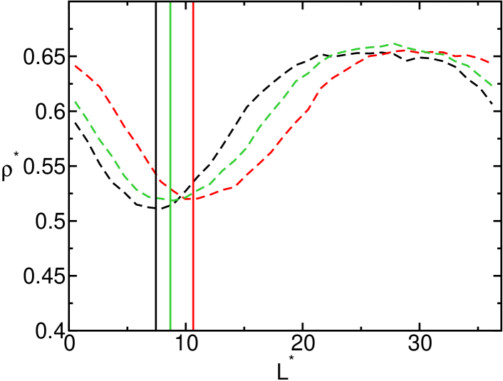
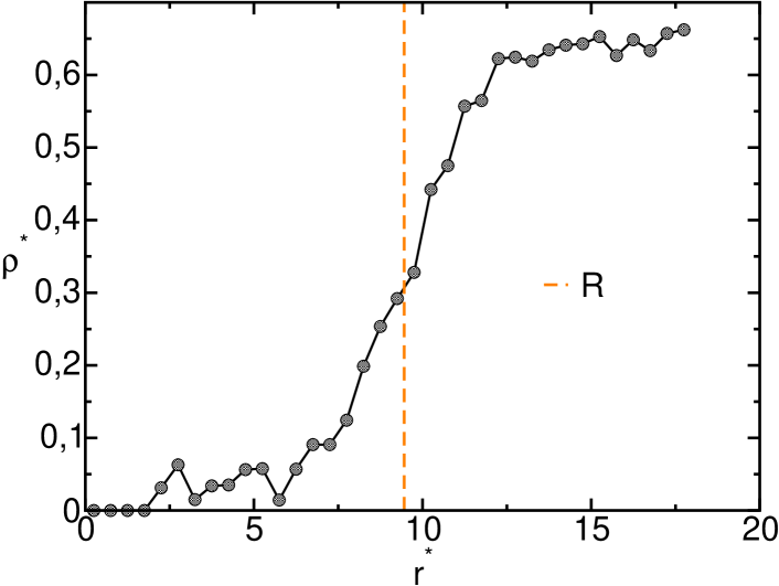
(a) (b)

Figure 2: (a) Density profiles along the $x$ (black), $y$ (red) and $z$ (green) coordinates of the simulation box. The bubble centre along each coordinate is located at the corresponding density profile minimum (indicated with vertical lines in the figure). (b) Radial density profile centred at the position identified in (a). The vertical dashed line indicates the bubble radius obtained, as described in our previous work seedingNpT , as the radius for which the density is average between that inside the bubble and that of the surrounding liquid.

IV.3 Preparation of the initial configuration

To induce a bubble of certain radius we take an equilibrated configuration of the liquid of density $\rho_{l}$ and $N_{0}$ particles at the temperature of interest and we randomly subtract $N_{-}$ particles. We estimate the number of particles needed to be erased in order to obtain a bubble with a certain intended radius, $R_{i}$, as:

$$N_{-}=\frac{4\pi\rho_{l}}{3}R_{i}^{3}.$$ (3)

Then, we are left with $N_{T}$ particles and we switch on a spherically symmetric step-like repulsive potential, $U_{rp}$, at a given point of the simulation box to create a cavity in the fluid:

$$U_{rp}=\frac{\epsilon_{rp}}{2}\sum_{i=1}^{i=N_{T}}\left[1-\tanh\left(\frac{r_{i-rp}-r_{rp}}{\alpha_{rp}}\right)\right].$$ (4)

Here, $r_{rp}$ and $\epsilon_{rp}$ are the radius and the height of the repulsive potential respectively, $r_{i-rp}$ is the distance between the centers of the repulsive potential and particle $i$ and $\alpha_{rp}$ controls the steepness of the repulsive step (we use $\alpha_{rp}^{*}=0.005$).

The precise value of the parameters of the repulsive potential are unimportant as long as the cavity is formed. For instance, we carried out simulations with a repulsive potential of radius $r_{rp}=5.0\sigma$ and $r_{rp}=3.5\sigma$, both with $\epsilon=1.0k_{B}T$ and the resulting bubbles were identical. This is due to the fact that the system minimizes the Helmholtz free energy, F, at constant N, V and T, which guarantees that the bubble size converges to an equilibrium value regardless the initial size of the cavity generated. $\epsilon_{rp}$ must be high enough to repel liquid particles from the repulsive potential area, but not too high to exert too strong forces in the particles leaving the repulsive area (otherwise pressure waves appear and it takes longer to equlibrate the system). We found $\epsilon_{rp}=1.0k_{B}T$ to be a good value.

In figure 3(a) we show the time evolution of the radius of the induced cavity. The repulsive potential is switched on at time 0. All these simulations are performed with a repulsive potential of $r_{rp}=5\sigma$ and $\epsilon_{rp}=1.0k_{B}T$. Cavities with different radii have been induced by erasing a different amount of particles from the simulation box. The corresponding intended radius, $R_{i}$ in Eq. 3, is reported in the figure legend. The correspondence between the radius of the generated cavity and $R_{i}$ is quite good. Obviously, when no particles are removed ($R_{i}^{*}=0$) the cavity radius is close to $r_{rp}$.

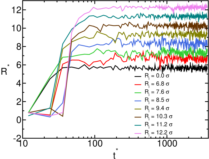
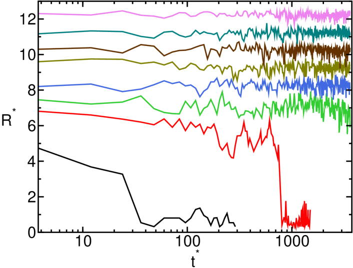
(a) (b)

Figure 3: (a)Radius of the cavity as a function of time. A repulsive step-like potential is switched on at the beginning of the simulation. Different cavity radii are obtained by subtracting different amount of particles to aim at a certain intended cavity radius ($R_{i}$ in the legend) according to Eq. 3. The simulation box edge in all cases is $L=36.7307\sigma$. (b) Continuation of the runs shown in (a) but with the repulsive potential switched off.

From the previous step we have configurations with the same simulation box edge, $L$, different number of particles and a cavity with a certain radius. In table 1 we give details on the systems employed in this work. Those with $L^{*}=36.73$ correspond to the simulations shown in Fig. 3.

IV.4 Critical bubble radius

We now switch off the repulsive potential and let the system equilibrate. In Fig. 3(b) we show the continuation of the simulations shown in Fig. 3(a) but switching off the repulsive potential at time 0. In most cases the cavity generated due to the repulsive potential remains stable throughout the simulation, i. e., we got equilibrated bubbles whose size is dictated by a minimisation of F in the system. The F minimum could be a local one and a cylindrical bubble pipe could form when the simulation is run for long times schrader2009simulation ; binder2012beyond , but we have not come across this problem. For $R_{i}^{*}=0$ the cavity immediately redissolved and we did not get any stable bubble. For $R_{i}^{*}=6.8$ the bubble remained stable for about $t^{*}=$750 and then redissolved. This is enough time to compute the bubble properties, as we show later on.

Not all trajectories with a stable bubble are suitable to obtain the bubble properties: it should also be possible to define bulk properties in the surrounding liquid. If the bubble is too big as compared to $L$, a too thin liquid layer will separate one bubble from its periodic replica. In Fig. 4(a) we show radial density profiles starting from the bubble centre of the simulations with a stable bubble. The curves shown in the figure are in reality fits of superimposed density profiles to the following sigmoid function:

$$\rho(r)=\frac{\rho_{v,dp}+\rho_{l,dp}}{2}+\left(\frac{\rho_{l,dp}-\rho_{v,dp}}{2}\right)\cdot\tanh\left[(r-R_{c})/\alpha\right],$$ (5)

where $\rho_{v,dp}$ and $\rho_{l,dp}$ are the densities of the vapor and the liquid phases obtained with the density profile (dp) fit respectively, $\alpha$ is a parameter related to the width of the interfacial region and $R_{c}$, our definition of the critical bubble radius, is the distance at which the density is the average between both phases (i. e. the “equi-density” critical radius in Ref. seedingNpT ):

$$\rho(R_{c})=\frac{\rho_{v,dp}+\rho_{l,dp}}{2}$$ (6)

The fit parameters $R_{c}$, $\rho_{l,dp}$ and $\rho_{v,dp}$ are reported in Table 1.

Due to periodic boundary conditions the density profiles can only be computed until $L/2$. Therefore, the fits shown in Fig. 4 are an extrapolation beyond $L/2$ (shown with dashed curves). As it can be seen in part (b) of the figure, for the two biggest bubbles, the liquid density has not converged by $L/2$, indicated by a vertical dashed line in the figure. In these cases the liquid does not reach a uniform bulk density along the directions perpendicular to the box sides. We can nonetheless define the liquid density via $\rho_{l,dp}$, which is a parameter of the fit above.

In Fig. 5 we show $\rho_{l,dp}$ as a function of the pressure obtained in the simulations with the virial equation (purple diamonds). These are compared with the red dots, which have been obtained in bulk liquid simulations. The agreement is quite satisfactory, which means that the nucleus is small as compared to the whole system and its presence does not affect the liquid density-pressure relation in any measurable manner. Thus, the thermodynamic state of the bulk liquid phase that surrounds the bubble can be estimated from the simulation that contains the bubble. Only small deviations between the bulk equation of state (red points) and that coming from the bubble simulations (purple diamonds) are present in the two biggest bubbles, which is perhaps expected from the afore-mentioned finite size effects in these cases.

To test if the obtained bubbles are indeed critical, we take a number of configurations obtained along the course of the simulation where the bubbles were stabilised and launch NPT simulations at the pressure given by the virial equation. We give an example of such test in Fig. 6, where we show the evolution of the bubble radius in NPT simulations for 30 bubble configurations with radius $\sim 9\sigma$ obtained in the NVT simulation corresponding to $R_{i}=9\sigma$ in Fig. 3(b). In this and all cases the bubbles grows/shrink in roughly half of the trajectories, which is a clear indication that critical bubbles are equilibrated in the NVT ensemble. Demonstrating that critical nuclei are equilibrated at constant NVT is the most important result of this work. Therefore, the bubbles that minimimize F at constant N, V and T correspond to a maximum of G at the same N, T and at constant P (that corresponding to the overall pressure in the system at constant V).

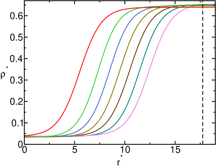
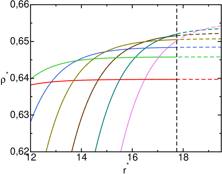
(a) (b)

Figure 4: (a) Fits to the radial density profiles of the stabilised bubbles (Eq. 5). The color code is the same as in Fig. 3. The vertical dashed line indicates a distance of half the edge of the simulation box. Beyond that distance the fits are an extrapolation and are shown in dashed curves. In part (b) a zoom close to that distance is shown.

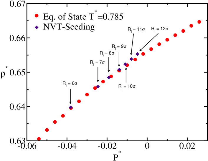
Figure 5: Bulk liquid density equation of state (red dots) compared with the density of the liquid surrounding the bubble, $\rho_{l,dp}$, versus the virial pressure of the whole system (purple diamonds).

$R_{i}$	$R_{c}$	$\rho_{v,dp}$	$P_{v,dp}$	$\rho_{l,dp}$	$P_{l,dp}$	$\rho_{v,cp}$	$P_{v,cp}$	$\Delta P$	$N_{0}$	$N_{T}$	$L$	$V_{box}/V_{bub}$	$\log(J)$
5.7	6.400	0.0320	0.0207	0.645	-0.0314	0.0345	0.0226	0.0540	32500	32000	37.1026	46.51	-17.07
6.8	5.506	0.0300	0.0197	0.640	-0.0380	0.0340	0.0222	0.0602	32000	31136	36.7307	70.87	-12.32
7.6	7.315	0.0327	0.0211	0.646	-0.0245	0.0355	0.0230	0.0341		30795		30.57	-22.23
8.5	8.466	0.0338	0.0218	0.648	-0.0191	0.0362	0.0233	0.0342		30342		19.63	-30.48
9.4	9.483	0.0340	0.0219	0.651	-0.0139	0.0369	0.0236	0.0375		29760		13.99	-37.74
10.3	10.48	0.0360	0.0231	0.652	-0.0109	0.0373	0.0238	0.0374		29034		10.39	-46.90
11.2	11.47	0.0365	0.0234	0.654	-0.0079	0.0376	0.0240	0.0319		28147		8.243	-56.42
12.2	12.44	0.0380	0.0243	0.655	-0.0049	0.0380	0.0242	0.0290		27082		6.493	-65.37
12.2	12.13	0.0375	0.0240	0.653	-0.0059	0.0379	0.0241	0.0300	136000	131072	59.2509	27.84	-62.62

Table 1: Details on the simulations used to compute the bubble nucleation rate for overstretched Lennard Jones fluids. All data are reported in reduced units. $R_{i}$ is the intended bubble radius (Eq. 3), $R_{c}$ is the critical bubble radius obtained in NVT-Seeding by fitting the radial density profile (dp) starting at the bubble center to Eq. 5, $\rho_{v,dp}$ and $\rho_{l,dp}$ are the vapor and the liquid number densities obtained from such fit, $P_{l,dp}$ ($P_{v,dp}$) is the liquid (vapor) pressure obtained from $\rho_{l,dp}$ ($\rho_{v,dp}$) and the bulk liquid (vapor) equation of state, $\rho_{v,cp}$ is the vapor density obtained by equating the chemical potential of the fluid to that of the vapor, $P_{v,cp}$ is the vapor pressure obtained from $\rho_{v,cp}$ and the bulk vapor equation of state, $\Delta P$ is $P_{v,cp}-P_{l,dp}$, $L$ is the length of the simulation box edge, $N_{T}$ is the number of particles in the simulation box (after deletion of $N_{-}$ particles from a system with $N_{0}$ particles), $V_{box}/V_{bub}$ is the volume ratio between the box and the bubble, and $J$ is the nucleation rate.

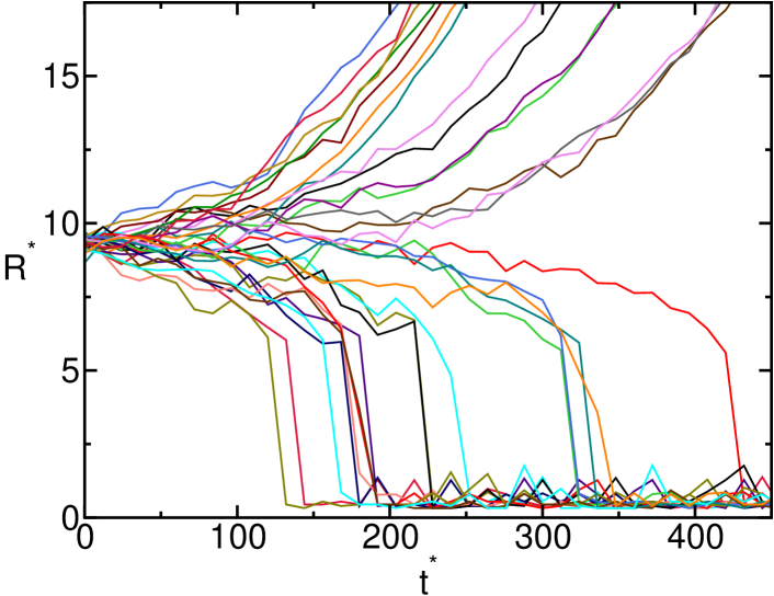
Figure 6: Bubble radius time evolution in the NPT ensemble for 30 configurations taken from an NVT simulation of an equilibrated bubble (that corresponding to $R_{i}^{*}=9$ in Fig. 3(b)). These simulations were launched at $T^{*}=0.785$ and $P^{*}=-0.014$ (the virial pressure of the NVT run where the bubble configurations were generated). The bubbles grow/shrink in roughly half of the trajectories, which proves that critical bubbles are obtained in the NVT simulations.

IV.5 Calculation of $\Delta P$

$\Delta P$ is the pressure difference between the vapor inside the critical bubble and that of the surrounding liquid. We obtain the liquid pressure through $\rho_{l,dp}$, the liquid density from the density profiles, and the bulk liquid equation of state that relates pressure with density (red dots in Fig. 5). Such pressure is reported in Table 1 as $P_{l,dp}$. To find the vapor pressure inside the critical bubble, we follow our previous approach seedingNpT and use the fact that the chemical potential of the liquid and the vapor phases are equal both at coexistence and at nucleation conditions tolman1949effect . The chemical potential difference with respect to coexistence at any pressure can be found by integrating the inverse density from the coexistence pressure, ($P^{*}_{coex}=0.026$ at $T^{*}=0.785$):

$$\Delta\mu(P)=\mu(P)-\mu_{coex}=\int_{P_{coex}}^{P}\frac{1}{\rho}dP$$ (7)

In Fig. 7 we show in black and red the pressure versus the chemical potential difference with coexistence for the vapor and the liquid respectively. For a given liquid pressure ($P_{l,dp}$) we obtain the vapor pressure by reading in Fig. 7(a) the vapor pressure for $\Delta\mu(P_{l,dp})$. We refer to this vapor pressure, obtained by chemical potential (cp) equality, as $P_{v,cp}$. Finally, $\Delta P$ is $P_{v,cp}-P_{l,dp}$. The values of $\Delta P$ thus obtained for the bubbles studied in this work are reported in Table 1 and plotted versus $P_{l,dp}$ in Fig. 7 (b) with red dots.

We could have obtained the vapor pressure via $\rho_{v,dp}$ (the density inside the bubble) and the vapor equation of state. The resulting vapor pressure, $P_{v,dp}$, is reported in table 1. We do not use $P_{v,dp}$ to compute $\Delta P$ because such vapor pressure value does not guarantee that the vapor chemical potential is equal to that of the surrounding liquid. In table 1 it can be seen that $P_{v,dp}$ is similar to $P_{v,cp}$, although systematically smaller. The difference arises from the discrepancy between the actual density near the center of the bubble and that of the hypothetical system. Consistently, the discrepancy increases as stretching (or the superheating) is increased and the bubbles become smaller. Therefore, computing the bubble pressure through $\rho_{v,dp}$ gives reasonable but not accurate or rigorous values.

In order to obtain a function that gives $\Delta P$ at any liquid pressure –which will be needed to fit $J$ along pressure– we do as follows: we fit the $P(\Delta\mu)$ data shown in Fig. 7(a) to a linear fit for the liquid and for the vapor. The difference between both fits gives $\Delta P$ as a function of $\Delta\mu$. Then, we substitute $\Delta\mu$ in the resulting expression by $\Delta\mu(P_{liquid})$. This gives $\Delta P(P_{liquid})$, that we represent in Fig. 7(b) with a black line.

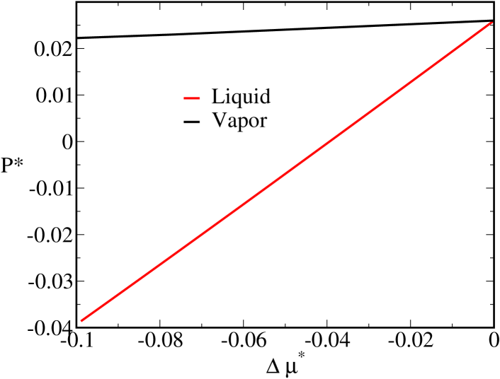
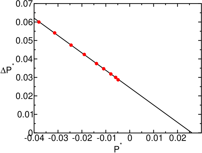
(a) (b)

Figure 7: (a) Pressure versus the chemical potential difference with respect to coexistence as obtained from Eq. 7 for the liquid and the vapor. (b) $\Delta P$ versus the liquid pressure. Red dots are the values of $\Delta P$ for the bubbles studied in this work.

IV.6 Nucleation rate

With Eq. 1 and the values reported in Table 1 for $\Delta P$, $\rho_{l,dp}$ and $R_{c}$ we obtain the nucleation rate, reported also in Table 1. The NVT-Seeding results for the nucleation rate are shown with pink solid circles in Fig. 8. These are compared with Seeding results in the NPT ensemble (brown dots), obtained as described in Ref. seedingNpT . The agreement between Seeding results in both ensembles is excellent. In Fig. 8 we also include with orange diamonds data obtained for the bubble nucleation rate in conditions of high overstretching where cavitation is spontaneous in a simulation starting from a bulk liquid configuration. In such conditions the rate can be estimated as $J=1/(Vt)$ filion:244115 , where $t$ is the average nucleation time in a handful of independent trajectories and $V$ is the system’s volume. The results for the nucleation rate obtained by brute force molecular dynamics are reported in table 2. Although Seeding cannot be directly used in conditions where cavitation is spontaneous given that the critical bubbles are too small, the trend of Seeding data is consistent with the spontaneous cavitation data.

$P^{*}$	-0.090	-0.082	-0.075
$log(J^{*})$	-6.33	-6.59	-6.95

Table 2: Nucleation rate in conditions of high overstretching, where the bubbles spontaneously nucleate in a brute force molecular dynamics simulation. All simulations have been run with a system of 32000 particles.

In a recent publication, we showed that when the bubble radius is measured with the definition adopted in this paper, NPT-Seeding gives bubble nucleation rates consistent with those computed by means of independent rare event simulation techniques seedingNpT . Here we demonstrate that NVT and NPT-Seeding give the same results. The advantage of NVT over NPT-Seeding is that the critical bubble is naturally equilibrated along the course of the simulation. In the NPT ensemble, however, the bubble either grows, if the pressure is lower than that for which the inserted bubble is critical, or shrinks in the contrary case. Thus, by performing simulations at different pressures, the pressure that makes the bubble critical is enclosed within a certain range. This procedure is much more cumbersome than just letting the critical bubble equilibrate by itself as we do in the NVT ensemble. Moreover, NPT-Seeding entails an error in the pressure that makes the bubble critical. By contrast, in the NVT ensemble the pressure is obtained from the density of the fluid surrounding the bubble, that can be accurately averaged along the course of the long NVT simulation in which the critical bubble is stable. Therefore, we recommend the NVT ensemble to compute bubble nucleation rates along isotherms via Seeding.

The only caveat for the use of Seeding in the NVT ensemble is the appearance of finite size effects when the bubble is big as compared to the simulation box. In practice, one should check that the fluid reaches a plateau density at $L/2$ from the bubble centre. In Fig. 2 we show that the two largest bubbles generated in a box with $L^{*}=36.73$ do not meet this requirement, so we anticipate that these systems might be affected by finite size effects. The rate corresponding to these systems is shown with empty circles in Fig.8. Finite size effects are not strong given that neither data clearly deviates from the general trend. We find that NVT-Seeding is a very promising strategy to enhance the efficiency and accuracy of Seeding. In our study finite size effects started to appear when the volume ratio between the simulation box and the critical bubble was smaller than $\sim 8$ (see Table 1). Further work is required to establish if the appearance of finite size effects in NVT-Seeding below this volume ratio is more general.

IV.7 Nucleation rate fit and surface tension

The pink curve in Fig. 8 is a CNT inspired fit to the NVT-Seeding data. To get such curve we need, according to Eq. 1, $\Delta P$, $\rho_{l}$ and $R_{c}$ as a function of pressure. $\rho_{l}$ and $\Delta P$ versus pressure have already been presented in Figs. 5 and 7 respectively. We have already evaluated $R_{c}$ for different pressures from the seeding simulations (see table 1). However, the dependence of $R_{c}$ with the liquid pressure is far from linear. Rather than directly fitting $R_{c}$ vs the liquid pressure, it is more convenient to get the surface tension dependence with pressure first through the Laplace equation $\gamma=\Delta PR_{c}/2$. The $\gamma$ values obtained from the $R_{c}$ and $\Delta P$ Seeding data combined with the Laplace equation are shown in Fig. 9(a). As expected from the good agreement for the nucleation rate, NPT and NVT-Seeding give the same $\gamma$. We observe that $\gamma$ decreases as the bubbles become smaller, in contrast with Ref. matsumoto2008nano where $\gamma$ was found to be roughly constant in NVT simulations of bubbles. The NVT-Seeding $\gamma$ data can be linearly fitted alongside the coexistence $\gamma$, $\gamma_{0}$ (green dot in the figure). We take $\gamma_{0}$ from our previous work seedingNpT . With $\gamma(P)$ and the Laplace equation we obtain $R_{c}$ at any liquid pressure. With that, we have all the ingredients required to fit $J$ (pink curve in Fig. 8).

If $\gamma$ is assumed to be equal to the coexistence value for any pressure (capillarity approximation) one gets the red curve in Fig. 8. As expected, the red curve is below the pink one given that the coexistence $\gamma$ is larger than those obtained by Seeding for overstretched fluids. Therefore, a theoretical description based on CNT and the capillarity approximation fails in predicting bubble nucleation rates.

Finally, we represent the $\gamma$ data shown in Fig. 9(a) as a function of $1/R_{c}$ in Fig. 9(b). The straight line is a fit to the following expression proposed by Tolman tolman1949effect :

$$\gamma=\gamma_{0}\left(1-2\delta_{T}/R_{c}\right),$$ (8)

where $\delta_{T}$ is the Tolman length, which sign tells if $\gamma$ increases or decreases with curvature at constant temperature and its magnitude indicates how strong is such variation kashchievbook ; blokhuis2006thermodynamic ; wilhelmsen2015tolman ; sampayo . In this case we obtain a positive $\delta_{T}$ (hence $\gamma$ decreases with curvature) of about the particle radius: $\delta_{T}^{*}=0.47$.

It is fair to point out here that the theoretical framework employed in this paper (the Laplace equation and Eqs. 1 and 8) assumes that the critical bubble radius is that corresponding to the surface of tension. In principle, such radius does not necessarily coincide with that obtained in our simulations as explained in section IV.4. However, in a recent study we found that such radius definition plus CNT provides free energy barrier heights consistent with those obtained from independent Umbrella Sampling calculations seedingvienes . This suggests that our radius definition provides a good estimate of the radius of tension. This idea is supported in this paper by the consistency between seeding and brute force data for the nucleation rate (see Fig. 8).

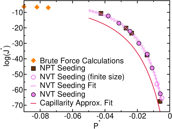
Figure 8: Nucleation rate as a function of the liquid pressure at constant temperature $T^{*}=0.785$. Pink and brown symbols correspond to Seeding data obtained in the NVT and NPT ensemble respectively. Empty symbols are data subject to finite size effects. Brute force calculations are shown as orange diamonds. Pink curve is a CNT fit (Eq. 1) to the NVT seeding data. The dashed pink curves indicate the upper and lower error limits in the solid one by considering an error of 0.1 $\sigma$ in $R_{c}$ and a relative error of 0.5 per cent in $\Delta P$. Red curve corresponds to a $J$ estimate based on the capillarity approximation (Eq. 1 assuming that $\gamma$ is equal to the coexistence $\gamma$ for any pressure).

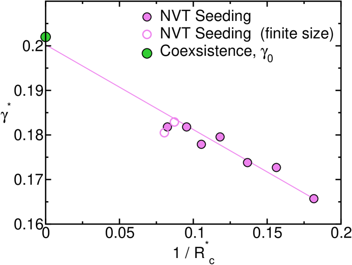
(a) (b)

Figure 9: (a)Interfacial free energy as a function of the liquid pressure. Pink (brown) circles (squares) correspond to NVT (NPT) Seeding simulations. The coexistence $\gamma$, shown with a green circle, was obtained in Ref. seedingNpT . The pink line is a linear fit to the coexistence value and the NVT-Seeding data. (b) $\gamma$ versus the inverse critical radius.

V Summary and conclusions

In this paper we study the nucleation of bubbles in overstretched Lennard Jones fluids at constant temperature. We first “seed” the fluid with a cavity by randomly removing particles and switching on a repulsive step-like potential. We then switch off the respulsive potential and let the system evolve at constant volume and temperature (NVT ensemble). The cavity becomes a vapor bubble in equilibrium with the surrounding liquid. We demonstrate that such bubble corresponds to the critical one at the thermodynamic conditions of the surrounding liquid. We measure the bubble radius by computing radial density profiles from its center and the vapor pressure by means of thermodynamic integration considering equal chemical potential between the bubble and the liquid. With the bubble radius and the pressure difference between both phases, we estimate the bubble nucleation rate using Classical Nucleation Theory to compute the free energy barrier height alongside an expression provided by Blander and Kats to estimate the kinetic pre-factor (Eq. 1). We name this approach to obtain the nucleation rate NVT-Seeding. To fit the computed nucleation rates we needed to consider a pressure dependent surface tension. Therefore, the capillarity approximation is not valid to make theoretical predictions of bubble nucleation.

The nucleation rate obtained by NVT-Seeding, here used for the first time, is fully consistent with that obtained by Seeding at constant pressure, NPT-Seeding, which is the approach adopted so far to study either bubble seedingNpT or crystal nucleation knottJACS2012 ; jacs2013 ; seedingvienes ; petersJACS2015 ; espinosaJCP2014 ; espinosaJCP2016 ; espinosaPRL2016 ; espinosaJPCL2017 ; guiomar ; sossoJCP2016 via Seeding. NVT-Seeding enables a more accurate computation of the critical bubble parameters than its NPT counterpart because the bubble remains stable along the course of the simulation. Moreover, given that the bubble equilibrates by itself, it is less cumbersome to apply. NVT-Seeding is quite handy to obtain the nucleation rate along pressure for a given temperature. However, to obtain the rate along an isobar NPT-Seeding is more suitable since in NVT-Seeding the pressure cannot be easily controlled because it is coupled to the bubble radius, which changes during the equilibration of the generated cavity. There are also size limitations in NVT-Seeding: too small bubbles will dissolve and too large ones will suffer from finite size effects due to the lack of surrounding liquid. More work is required to establish the applicability limits of the NVT-Seeding technique and to test if it is also valid to study nucleation in other sorts of phase transitions such as freezing or condensation.

VI Acknowledgments

This work was funded by grant FIS2016/78117-P of the MEC. C. Valeriani thanks financial support from FIS2016-78847-P of the MEC. The authors acknowledge the computer resources and technical assistance provided by the RES. P. R. thanks a doctoral grant from UCM.

References

- (1) J. S. van Duijneveldt and D. Frenkel, “Computer simulation study of free energy barriers in crystal nucleation,” J. Chem. Phys., vol. 96, p. 4655, 1992.
- (2) R. P. Sear, “Nucleation: theory and applications to protein solutions and colloidal suspensions,” Journal of Physics: Condensed Matter, vol. 19, no. 3, p. 033101, 2007.
- (3) J. Anwar and D. Zahn, “Uncovering molecular processes in crystal nucleation and growth by using molecular simulation,” Angewandte Chemie International Edition, vol. 50, no. 9, pp. 1996–2013, 2011.
- (4) G. C. Sosso, J. Chen, S. J. Cox, M. Fitzner, P. Pedevilla, A. Zen, and A. Michaelides, “Crystal nucleation in liquids: Open questions and future challenges in molecular dynamics simulations,” Chemical Reviews, vol. 116, no. 12, pp. 7078–7116, 2016.
- (5) I. Coluzza, J. Creamean, M. J. Rossi, H. Wex, P. A. Alpert, V. Bianco, Y. Boose, C. Dellago, L. Felgitsch, J. Fröhlich-Nowoisky, et al., “Perspectives on the future of ice nucleation research: Research needs and unanswered questions identified from two international workshops,” Atmosphere, vol. 8, no. 8, p. 138, 2017.
- (6) K. F. Kelton, Crystal Nucleation in Liquids and Glasses. Boston: Academic, 1991.
- (7) R. J. Allen, P. B. Warren, and P. R. ten Wolde, “Sampling rare switching events in biochemical networks,” Phys. Rev. Lett., vol. 94, p. 018104, 2005.
- (8) A. Haji-Akbari and P. G. Debenedetti, “Direct calculation of ice homogeneous nucleation rate for a molecular model of water,” Proceedings of the National Academy of Sciences, vol. 112, no. 34, pp. 10582–10588, 2015.
- (9) P. G. Bolhuis, D. Chandler, C. Dellago, and P. L. Geissler, “Transition path sampling: Throwing ropes over rough mountain passes, in the dark,” Annual review of physical chemistry, vol. 53, no. 1, pp. 291–318, 2002.
- (10) D. Moroni, P. R. ten Wolde, and P. G. Bolhuis, “Interplay between structure and size in a critical crystal nucleus,” Phys. Rev. Lett., vol. 94, p. 235703, 2005.
- (11) D. Quigley and P. M. Rodger, “Metadynamics simulations of ice nucleation and growth,” J. Chem. Phys., vol. 128, no. 15, p. 154518, 2008.
- (12) A. Laio and M. Parrinello, “Escaping free-energy minima,” Proc. Natl. Acad. Sci., vol. 99, p. 12562, 2002.
- (13) X.-M. Bai and M. Li, “Calculation of solid-liquid interfacial free energy: A classical nucleation theory based approach,” J. Chem. Phys., vol. 124, no. 12, p. 124707, 2006.
- (14) R. G. Pereyra, I. Szleifer, and M. A. Carignano, “Temperature dependence of ice critical nucleus size,” J. Chem. Phys., vol. 135, p. 034508, 2011.
- (15) B. C. Knott, V. Molinero, M. F. Doherty, and B. Peters, “Homogeneous nucleation of methane hydrates: Unrealistic under realistic conditions,” J. Am. Chem. Soc., vol. 134, pp. 19544–19547, 2012.
- (16) E. Sanz, C. Vega, J. R. Espinosa, R. Caballero-Bernal, J. L. F. Abascal, and C. Valeriani, “Homogeneous ice nucleation at moderate supercooling from molecular simulation,” Journal of the American Chemical Society, vol. 135, no. 40, pp. 15008–15017, 2013.
- (17) J. R. Espinosa, C. Vega, C. Valeriani, and E. Sanz, “Seeding approach to crystal nucleation,” J. Chem. Phys., vol. 144, p. 034501, 2016.
- (18) M. Volmer and A. Weber, “Keimbildung in ubersattigten gebilden,” Z. Phys. Chem., vol. 119, p. 277, 1926.
- (19) R. Becker and W. Doring, “Kinetische behandlung der keimbildung in ubersattigten dampfen,” Ann. Phys., vol. 416, pp. 719–752, 1935.
- (20) N. E. Zimmermann, B. Vorselaars, J. R. Espinosa, D. Quigley, W. R. Smith, E. Sanz, C. Vega, and B. Peters, “Nacl nucleation from brine in seeded simulations: Sources of uncertainty in rate estimates,” The Journal of chemical physics, vol. 148, no. 22, p. 222838, 2018.
- (21) P. Rosales-Pelaez, M. Garcia-Cid, C. Valeriani, C. Vega, and E. Sanz, “Seeding approach to bubble nucleation in superheated lennard-jones fluids,” Physical Review E, vol. 100, no. 5, p. 052609, 2019.
- (22) L. G. MacDowell, V. K. Shen, and J. R. Errington, “Nucleation and cavitation of spherical, cylindrical, and slablike droplets and bubbles in small systems,” The Journal of chemical physics, vol. 125, no. 3, p. 034705, 2006.
- (23) P. Koß, A. Statt, P. Virnau, and K. Binder, “Free-energy barriers for crystal nucleation from fluid phases,” Physical Review E, vol. 96, no. 4, p. 042609, 2017.
- (24) A. Statt, P. Virnau, and K. Binder, “Finite-size effects on liquid-solid phase coexistence and the estimation of crystal nucleation barriers,” Physical review letters, vol. 114, no. 2, p. 026101, 2015.
- (25) J. Wedekind, D. Reguera, and R. Strey, “Finite-size effects in simulations of nucleation,” The Journal of Chemical Physics, vol. 125, no. 21, p. 214505, 2006.
- (26) M. Shusser and D. Weihs, “Explosive boiling of a liquid droplet,” International journal of multiphase flow, vol. 25, no. 8, pp. 1561–1573, 1999.
- (27) M. Shusser, T. Ytrehus, and D. Weihs, “Kinetic theory analysis of explosive boiling of a liquid droplet,” Fluid Dynamics Research, vol. 27, no. 6, p. 353, 2000.
- (28) A. Toramaru, “Vesiculation process and bubble size distributions in ascending magmas with constant velocities,” Journal of Geophysical Research: Solid Earth, vol. 94, no. B12, pp. 17523–17542, 1989.
- (29) H. Massol and T. Koyaguchi, “The effect of magma flow on nucleation of gas bubbles in a volcanic conduit,” Journal of volcanology and geothermal research, vol. 143, no. 1-3, pp. 69–88, 2005.
- (30) C. E. Brennen, Cavitation and bubble dynamics. Cambridge University Press, 2014.
- (31) K. S. Suslick, “Sonochemistry,” science, vol. 247, no. 4949, pp. 1439–1445, 1990.
- (32) K. S. Suslick, M. M. Mdleleni, and J. T. Ries, “Chemistry induced by hydrodynamic cavitation,” Journal of the American Chemical Society, vol. 119, no. 39, pp. 9303–9304, 1997.
- (33) G. Kähler, F. Bonelli, G. Gonnella, and A. Lamura, “Cavitation inception of a van der waals fluid at a sack-wall obstacle,” Physics of Fluids, vol. 27, no. 12, p. 123307, 2015.
- (34) Z.-J. Wang, C. Valeriani, and D. Frenkel, “Homogeneous bubble nucleation driven by local hot spots: A molecular dynamics study,” The Journal of Physical Chemistry B, vol. 113, no. 12, pp. 3776–3784, 2008.
- (35) S. L. Meadley and F. A. Escobedo, “Thermodynamics and kinetics of bubble nucleation: Simulation methodology,” The Journal of chemical physics, vol. 137, no. 7, p. 074109, 2012.
- (36) Blander, Milton, and Joseph L. Katz. , “Bubble nucleation in liquids.,” AIChE Journal, vol. 21, no. 5, pp. 833–848, 1975.
- (37) K. K. Tanaka, H. Tanaka, R. Angelil, and J. Diemand, “Simple improvements to classical bubble nucleation models,” Physical review E, vol. 92, no. 2, p. 022401, 2015.
- (38) S. Plimpton J. Comput. Phys., vol. 117, p. 1, 1995.
- (39) R. W. Hockney, S. P. Goel, and J. Eastwood, “Quiet high resolution computer models of a plasma,” J. Comp. Phys., vol. 14, pp. 148–158, 1974.
- (40) S. Nos , “A unified formulation of the constant temperature molecular dynamics methods,” J. Chem. Phys., vol. 81, p. 511, 1984.
- (41) M. Schrader, P. Virnau, and K. Binder, “Simulation of vapor-liquid coexistence in finite volumes: A method to compute the surface free energy of droplets,” Physical Review E, vol. 79, no. 6, p. 061104, 2009.
- (42) K. Binder, B. J. Block, P. Virnau, and A. Tröster, “Beyond the van der waals loop: What can be learned from simulating lennard-jones fluids inside the region of phase coexistence,” American Journal of Physics, vol. 80, no. 12, pp. 1099–1109, 2012.
- (43) R. C. Tolman, “The effect of droplet size on surface tension,” The journal of chemical physics, vol. 17, no. 3, pp. 333–337, 1949.
- (44) L. Filion, M. Hermes, R. Ni, and M. Dijkstra, “Crystal nucleation of hard spheres using molecular dynamics, umbrella sampling, and forward flux sampling: A comparison of simulation techniques,” J. Chem. Phys., vol. 133, no. 24, p. 244115, 2010.
- (45) M. Matsumoto and K. Tanaka, “Nano bubble-size dependence of surface tension and inside pressure,” Fluid dynamics research, vol. 40, no. 7-8, p. 546, 2008.
- (46) D. Kashchiev, Nucleation: Basic Theory with Applications. Oxford: Butterworth-Heinemann, 2000.
- (47) E. M. Blokhuis and J. Kuipers, “Thermodynamic expressions for the tolman length,” The journal of chemical physics, vol. 124, no. 7, p. 074701, 2006.
- (48) Ø. Wilhelmsen, D. Bedeaux, and D. Reguera, “Tolman length and rigidity constants of the lennard-jones fluid,” The Journal of chemical physics, vol. 142, no. 6, p. 064706, 2015.
- (49) J. G. Sampayo, A. Malijevskỳ, E. A. Müller, E. de Miguel, and G. Jackson, “Communications: Evidence for the role of fluctuations in the thermodynamics of nanoscale drops and the implications in computations of the surface tension,” J. Chem. Phys., vol. 132, no. 14, p. 141101, 2010.
- (50) N. E. R. Zimmermann, B. Vorselaars, D. Quigley, and B. Peters, “Nucleation of NaCl from aqueous solution: Critical sizes, ion-attachment kinetics, and rates,” Journal of the American Chemical Society, vol. 137, no. 41, pp. 13352–13361, 2015.
- (51) J. R. Espinosa, E. Sanz, C. Valeriani, and C. Vega, “Homogeneous ice nucleation evaluated for several water models,” J. Chem. Phys., vol. 141, p. 18C529, 2014.
- (52) J. R. Espinosa, C. Navarro, E. Sanz, C. Valeriani, and C. Vega, “On the time required to freeze water,” The Journal of Chemical Physics, vol. 145, no. 21, p. 211922, 2016.
- (53) J. R. Espinosa, A. Zaragoza, P. Rosales-Pelaez, C. Navarro, C. Valeriani, C. Vega, and E. Sanz, “Interfacial free energy as the key to the pressure-induced deceleration of ice nucleation,” Phys. Rev. Lett., vol. 117, p. 135702, 2016.
- (54) J. R. Espinosa, G. D. Soria, J. Ramirez, C. Valeriani, C. Vega, and E. Sanz, “Role of salt, pressure, and water activity on homogeneous ice nucleation,” J. Phys. Chem. Lett., vol. 8, p. 4486, 2017.
- (55) G. D. Soria, J. R. Espinosa, J. Ramirez, C. Valeriani, C. Vega, and E. Sanz, “A simulation study of homogeneous ice nucleation in supercooled salty water,” The Journal of chemical physics, vol. 148, no. 22, p. 222811, 2018.
- (56) G. C. Sosso, G. A. Tribello, A. Zen, P. Pedevilla, and A. Michaelides, “Ice formation on kaolinite: Insights from molecular dynamics simulations,” The Journal of Chemical Physics, vol. 145, no. 21, p. 211927, 2016.