On microscopic theory of pygmy- and giant resonances

Abstract

The Green function formalism with a consistent account for phonon coupling (PC), based on the self-consistent theory of finite Fermi-systems, is applied for pygmy- and giant multipole resonances in magic nuclei with the aim to consider particle-hole (ph) and complex 1p1h$\otimes$phonon configurations. A new equation for the effective field, which describes nuclear polarizability, is obtained. It contains new PC contributions which are of interest in the energy region under consideration. They are due to: i)the tadpole effect in the standard ph-propagator, ii)two new induced interactions (caused by the exchange of ph-phonon) in the second ph-channel and in the particle-particle channels, and iii) the first and second variations of the effective interaction in the phonon field. The general expressions for energies and probabilities of transitions between the ground and excited states are obtained. The qualitative analysis and discussion of the new terms are performed.

I introduction

The modern microscopic theory of pygmy- and giant multipole resonances (for simplicity, hereafter PDR and GMR) is mainly at the level of accounting for: i) self-consistency between the mean field and effective interaction and ii) the low-lying phonon coupling (PC) Paar ; Bracco ; kaevYadFiz2019 . First of all, accounting for PC explained the third integral GMR characteristic, i.e. the width revKST ; Paar ; ave2011 . The self-consistency approach turned out very useful for astrophysical applications even at QRPA level due to its great predictive power Goriely . Also, PC inclusion resulted in considerable improvement in explanations of GMRs properties and appropriate applications Paar ; Bracco ; kaevYadFiz2019 ; YadFiz2011 , although some problems are encountered even for magic nuclei. For example, the ones connected with the Skyrme parameters Tselyev2016 and spin-spin forces Lyutor2018 universal for all nuclei.

As far as PDR is concerned, the situation is more complex and requires more detailed consideration. Firstly, it is due to existence of many new and delicate physical effects in this energy region, like irrotational and vortical kind of motion (the toroidal dipole resonance which is present in all the nuclei, while PDR manifests itself in the nuclei with N$>$Z Nester ; Bracco ; Paar ), and the upbend phenomenon Larsen at 1-3 MeV energy region. Besides, there are new experimental possibilities Cosel ; Larsen ; Bracco , for example, polarized proton inelastic scattering at very forward angles Cosel . Secondly, as it turned out, it is impossible to explain completely the observed PDR fine structure within the latest self-consistent approach with Skyrme functional and accounting for PC Lyutor2018 in the nucleus ²⁰⁸Pb, which was always a polygon for theory and experiment in PDR and GMR fields. All these facts can be a real reason for an additional analysis of PDR and GMR microscopic theory.

In the field of the self-consistent description of characteristics of ground and low-lying collective states, large work and a lot of succesful calculations have been performed by the Kurchatov Institute group, see reviews SapTol2016 ; kaevYadFiz2019 . Here the self-consistent theory of finite Fermi systems (TFFS) KhSap1982 , based on the effective density functional theory, has been used with Fayans functional Fayans and PC. In this sense, one can speak about the second stage of developing TFFS. It was shown that in all the numerous problems considered, PC contribution is sizable, of fundamental importance and necessary for explaining experimental data. The success of these works is explained not only by the use of Fayans functional but also by a more consistent consideration of PC effects, in particular, the tadpole effects KhSap1982 ; SapTol2016 and, probably, the effect of variation of the effective interaction in the phonon field voitenkov . The important reason for this success, in the author’s opinion, was the use of consistent quantum many-body formalism, the Green function (GF) method Migdal , to be exact.

Simultaneously with the above-mentioned GF approach KhSap1982 and beginning from 1983 kaev83 , the theory for PDR and GMR was being developed within GF method and with PC, in the framework of both non-selfconsistent kaev83 ; ts89 ; revKST and self-consistent variants ts2007 ; ave2011 . The difference between kaev83 and ts89 consisted in the fact that in ts89 the disadvantage of kaev83 was eliminated, namely, a special approximate method of chronological decoupling of diagrams (MCDD) (or, in a more modern terminology, time blocking approximation (TBA)) was developed in order to solve the problem of second order poles in the generalized propagator of the extended RPA propagator in kaev83 . This disadvantage was not important to explain the properties of M1 resonance ktZPhys , but it was important for electrical MGR. Later on, this method to solve the second order poles problem was considerably improved ts2007 so that the approach obtained the name of qasiparticle time blocking approximation (QTBA) for nuclei with pairing. See, for example, ts2018 for references to the improved TBA approaches for magic nuclei. However, the main physical content, i.e. inclusion of PC only into the particle-hole (ph) propagator (in the language of TFFS) has been always preserved despite the fact that the derivation method was different and was based on the Bethe-Salpeter equation. In particular, even the known tadpole effect was not considered in the generalized propagator of MCDD or TBA, except for the analytical attempt in YadFiz2011 , where this effect was considered within the method of kaev83 .

Thus, in contrast to what we have within the non-selfconsistent Sol89 and self-consistent scQPM quasiparticle–phonon model, where both energy regions (low-lying and PDR+GMR) are considered on an equal footing, there still exists a gap between GF approaches applied in the region of the ground state and low-lying excited states KhSap1982 ; SapTol2016 , on the one hand, and the approach in (PDR+GMR) energy region YadFiz2011 ; ave2011 , on the other hand. In any case, we are sure that the possibilities of GF approach have not been used completely in the microscopic theory of PDR and GMR.

The goal of this article is to use the GF approach based on the self-consistent TFFS, in the PDR+GMR energy region, in order to close this gap and to include PC consistently, i.e. not only into the ph-propagator but also into other quantities contained in GF apparatus, for example, the effective interaction. We will see that such an approach gives new effects, which can be important for the microscopic description of PDR and GMR.

In this article, we will consider only magic nuclei and complex configurations 1p1h$\otimes$phonon and discuss only $g^{2}$ PC corrections, where $g$ is the phonon creation amplitude. As usual, we use the fact of existence of the small $g^{2}$ parameter. Very often we symbolically write our formulas, the main of which are represented in the form of Feynman diagrams, so the final formulas can be easily obtained.

II Some earlier results with PC

As it was mentioned in the Introduction, the physical content of the previous GF approaches in the PDR and GMR theory was that $g^{2}$ PC corrections were included into ph-propagator, so that the new ph-propagator should correspond to the diagrams which are presented in Fig.1,

Figure 1: Diagrams corresponding to the simplest ph propagator with PC .

where the first diagram means the RPA case with the ph propagator

$$A_{12}(\omega)=\int G_{1}(\varepsilon+\frac{\omega}{2})G_{2}(\varepsilon-\frac{\omega}{2})d\varepsilon$$ (1)

Hereinafter number 2 before a graph or a corresponding formula means that there are two graphs or formulas of a similar type, low indices mean the set of single-particle quantum numbers 1 $\equiv({n_{1},j_{1},l_{1},m_{1}})$ , $\omega$ is the energy of the external field $V^{0}$ and we write everywhere $d\varepsilon$ instead of $\frac{d\varepsilon}{2\imath\pi}$. Of course, it is always necessary to keep in mind that for numerical results the method of MCDD ts89 or TBA in the case under consideration should be used in reality to avoid the above-mentioned problem with second order poles in the ph propagator shown in Fig.1. Such a generalized propagator is rather complicated, it was discussed in details and given in revKST .

In the works, performed within the self-consistent TFFS, the $g^{2}$ PC corrections to the mean field, which take into account the tadpole, have been used actively. They can be written in the symbolic form as

$$\delta\Sigma=gDGg+g_{11}D$$ (2)

and shown in Fig.2.

Figure 2: The $g^{2}$ corrections to the mean field. Straight and wavy lines correspond to GF G and D, circles with one wavy line stand for the amplitude of phonon production g, and the circle with two wavy lines is $g_{11}$

Here G and D are the single-particle and phonon GF’s:

$$G_{1}(\varepsilon)=\frac{1-n_{1}}{\varepsilon-\varepsilon_{1}+\imath\gamma}+\frac{n_{1}}{\varepsilon-\varepsilon_{1}-\imath\gamma},$$

$$D_{s}(\omega)=\frac{1}{\omega-\omega_{s}+\imath\gamma}-\frac{1}{\omega+\omega_{s}-\imath\gamma}$$ (3)

and g obeys the homogeneous equation Migdal

$$g=FAg$$ (4)

where F is the effective interaction , A is the ph propagator, Eq.(1). Eq.(4) means the RPA approach formulated in GF language.

The amplitude of creation of two phonons (similar in the tadpole case) is obtained as the variation of Eq.(4) in the field of phonon 2

$$g_{12}\equiv\delta^{(1)}g_{2}=\delta^{(1)}FAg_{1}+F\delta^{(1)}Ag_{1}+FAg_{12}$$ (5)

The solution of this equation is rather difficult. It has been solved only in the coordinate representation in the works by A.P. Platonov pertaining to other problems connected with the properties of ground or low-lying collective states platonov ; KhSap1982 . However, it is possible to use a realistic estimation of the two-phonon creation amplitude $g_{11}\equiv\delta^{(1)}g_{1}$, which is contained in the tadpole term. This estimation has been based on the approximation for the quantity $\delta F$ KhSap1982 :

$$\delta F=(\raisebox{1.0pt}{$\delta F$}\big{/}\raisebox{-1.0pt}{$\delta\rho$})\,Ag$$ (6)

If one neglects the small in-volume term of the amplitude g, a simple expression for $(g_{11})_{ik}=\alpha_{L}^{2}\partial^{2}U/\partial\textbf{r}_{i}\partial\textbf{ r}_{k}$ in the non-pole term $K^{ph}=\int d\omega g_{11}D(\omega)$ can be obtained platonov , where $U$ is the self-consistent mean field and $\alpha_{L}$ is the deformation parameter of the L-phonon in the Bohr-Mottelson model .

III Equation for new effective field $\tilde{V}$ with PC corrections

Our aim is to find $g^{2}$-corrections to the vertex $V$, which is described by the standard TFFS equation Migdal

$$V=e_{q}V^{0}+FAV$$ (7)

in order to find, within the GF method, a new equation for a new vertex, which takes into account all the $g^{2}$ corrections to $V$.

We assume that our approach is self-consistent, i.e. the mean field and effective interaction $F$ are defined, respectively, as the first and second functional derivations of the effective density functional. In this sense, our approach is a generalization of the self-consistent TFFS with PC corrections to the PDR and GMR energy region.

Using the general analogy for obtaining Eq.(5) and above-mentioned $g^{2}$-correction to the mean field, one can write the following for $g^{2}$-corrections to the vertex $V$:

$$\tilde{V}=V+\Delta V(g,V)$$ (8)

and

$$\Delta V=2gDG\delta^{(1)}V+\delta^{(2)}VD,$$ (9)

where the quantities $\delta^{(1)}V$ and $\delta^{(2)}V$ are the first and second order variations of the vertex $V$, Eq.(7) in the phonon field. They are shown in Fig.3. The second term in Eq.(9),Fig.3, contains ”pure” $g^{2}$ corrections, which are, in a sense, similar to the tadpole corrections in Fig.1, while the first term in Eq.(9),Fig.3, is a mix between the first order correction to the vertex $V$ and the ”end” correction of the first order in $g$, with the ends of the first diagram in Fig.3. kept in mind.

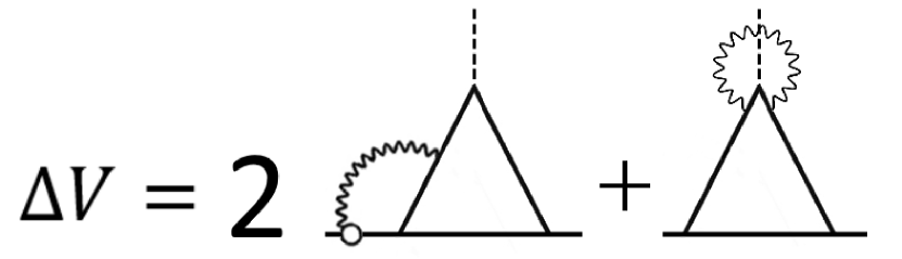
Figure 3: The $g^{2}$ corrections to the vertex V.

In fact, the corrections $\Delta V$ already appeared in the consideration of quite another problem, namely, the calculations of $g^{2}$ corrections to matrix elements $(\varphi_{\lambda_{1}},V\varphi_{\lambda_{2}})$ for static electromagnetic moments of odd nuclei in the ground state YadFiz2014 ; JPhysG . This problem was reduced to the analysis of 8 terms with $g^{2}$ corrections, from which 5 terms contain $\delta^{(2)}\varphi_{\lambda}$ (the so-called ends corrections) and the other 3 terms are our corrections $\Delta V$, Eg.(9), but in the static form, while in our case we need them at PDR and GMR energies. It turned out that these 5 terms, which depend strongly on single-particle ends $\lambda_{1}$ and $\lambda_{2}$, cancel each other noticeably, so that their algebraic sum gives an improvement to describe experimental data under consideration. For some particular cases, the other 3 corrections were estimated and it was shown that for the problems considered in YadFiz2014 ; JPhysG the appropriate $g^{2}$ corrections should not be addressed because they are important not for individual states $\lambda_{1}=\lambda_{2}$, but for the case when they contain large sums of small contributions. However, just this latter case of large sums of small contributions is of great interest for us when only the collective (or ”cooperative” Bracco ) phenomena like PDR and GMR are studied. It is well known that the collectivity of PDR and GMR are due to cogerent sums of many configurations 1p1h + (1p1h$\otimes$phonon)

Getting back to our problem, let us find the variations $\delta^{(1)}V$ and $\delta^{(2)}V$. But first, we obtain the quantity $\delta^{(2)}A$ for our case of similar phonons, which is contained in $\delta^{(2)}V$. For the general case, $\delta^{(2)}A$ is as follows:

$$\delta^{(2)}A=\delta^{(2)}G_{1}G_{2}=\delta^{\tilde{2}}\delta^{\tilde{1}}G_{1}G_{2},$$ (10)

where $\delta^{\tilde{1}}$ is variation in the field of phonon 1, and we have introduced notion $\tilde{1}$ for phonon 1, not to confuse it with the single-particle index 1. Then we have

$$\delta^{\tilde{1}}G_{1}G_{2}=\delta^{\tilde{1}}G_{1}G_{2}+G_{1}\delta^{\tilde{1}}G_{2}=$$

$$G_{1}g_{\tilde{1}}G_{3}G_{2}+G_{1}G_{2}g_{\tilde{1}}G_{3}$$ (11)

$$\delta^{\tilde{2}}G_{1}g_{\tilde{1}}G_{3}G_{2}=\delta^{\tilde{2}}G_{1}g\delta^{\tilde{1}}G_{3}G_{2}+G_{1}\delta^{\tilde{2}}g_{\tilde{1}}G_{3}G_{2}+$$

$$G_{1}g_{\tilde{1}}\delta^{\tilde{2}}G_{3}G_{2}+G_{1}g_{\tilde{1}}G_{3}\delta^{\tilde{2}}G_{2}$$ (12)

and analogically for the second term in Eq.(11). Finally, for the case $\tilde{1}=\tilde{1}$, which is of interest in our case for the variation $\delta^{(2)}V=\delta^{\tilde{1}}\delta^{\tilde{1}}V$, we obtain five terms instead of eight, they are shown in Fig.4.

$$\delta^{\tilde{1}}\delta^{\tilde{1}}G_{1}G_{2}=2G_{1}g_{\tilde{1}}G_{3}g_{\tilde{1}}G_{4}G_{2}+$$

$$2G_{1}g_{\tilde{1}\tilde{1}}G_{3}G_{2}+G_{1}g_{\tilde{1}}G_{3}G_{2}g_{\tilde{1}}G_{4}$$ (13)

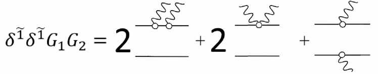
Figure 4: Expression (13) in the diagrammatic representation.

The quantities $\delta^{(1)}V$ and $\delta^{(2)}V$ should be obtained by variation of Eq.(7) in the phonon field:

$$\delta^{(1)}V= \delta^{(1)}FAV+F\delta^{(1)}AV+FA\delta^{(1)}V,$$

$$\delta^{(2)}V= \delta^{(1)}\delta^{(1)}V=F\delta^{(2)}AV+$$

$$2\delta^{(1)}F\delta^{(1)}AV+2\delta^{(1)}FA\delta^{(1)}V+2F\delta^{(1)}A\delta^{(1)}V+$$

$$\delta^{(2)}FAV+FA\delta^{(2)}V$$ (14)

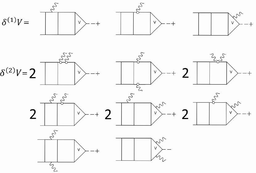
Figure 5: First- and second order variations of Eq.(7) in the phonon field.

They are shown in Fig.5, where the term with $\delta^{(2)}A$ is already shown by the three graphs in the first line for $\delta^{(2)}V$.

One can see from Eq.(14),Fig.5, that the quantities $\delta^{(1)}V$ and $\delta^{(2)}V$ obey a rather complicated coupled system of integral equations, the first of which has two free terms and the second one has five free terms. All these free terms contain the vertex $V$ or (in the case of $\delta^{(2)}V$) the quantity $\delta^{(1)}V$. System (14) can be solved if to use the approximation Eq.(6)for $\delta^{(1)}F$ and develop such an approximation for $\delta^{(2)}F$ further. However, this is a very complicated way and for the better understanding of physical sense, it is better here to use only above-mentioned free terms of Eq.(14). Also, one can transform Eq.(14) in order to find expressions for $\delta^{(1)}V$ and $\delta^{(2)}V$. However, in this case we will obtain a noticeable complication because of appearance of a two-phonon channel. We will not use this way for simplicity and because of our restriction to only complex 1p1h$\otimes$phonon configurations mentioned in the Introduction.

Let us go back to expression (8). One can see that expression (8) is the first iteration of the following equation (if $V$ , Eq.(7) is zero iteration)

$$\tilde{V}=V+\Delta V(g,\tilde{V}).$$ (15)

Then, after setting of the above-mentioned free terms of Eq.(14) and keeping in mind Eq.(15), we obtain the final equation for the new effective field $\tilde{V}$:

$$\tilde{V}=e_{q}V^{0}+FA\tilde{V}+2FGgDGgGG\tilde{V}+FGgGDGgG\tilde{V}$$

$$+2FGg_{\tilde{1}\tilde{1}}DGG\tilde{V}+4gGDFGgGG\tilde{V}+$$

$$+4FGgDGGFGgGG\tilde{V}+$$

$$+2g\delta FDGGG\tilde{V}+2\delta FDGgGG\tilde{V}+$$

$$2\delta FDGGFGgG\tilde{V}+2FGgDGG\delta FGG\tilde{V}+$$

$$2\delta FDGG\delta FGG\tilde{V}+\delta^{(2)}FDGG\tilde{V}$$ (16)

It is shown in Fig.6. The lines of Eq. (16) and Fig.6 correspond to each other. Because of the symbolical form of Eq.(16), in each of its lines 2 and 3, we have shown two graphs in Fig.6 instead of the terms with number 4 in the same lines of Eq.(16) All the terms in Eq. (16) correspond to the case when only the complex configurations 1p1hx$\otimes$phonon are taken into account in magic nuclei.

Thus, we have obtained that all the terms in the first line of Eq.(16),Fig.6, correspond to the previous approach kaev83 ; ts89 ; Tselyev2016 , which uses the ph-propagator with PC shown in Fig.1. The other lines contain the following difference from this approach. Namely, these are contributions due to: i) tadpole effect in the standard particle-hole propagator (the first term of the second line), ii) two new induced interactions ( due to exchange by the usual particle-hole phonon) in the second particle-hole channel and in the particle-particle channels (the second and third lines), and iii) the first and second variations of the effective interaction in the phonon field (the forth, fifth and sixth lines).

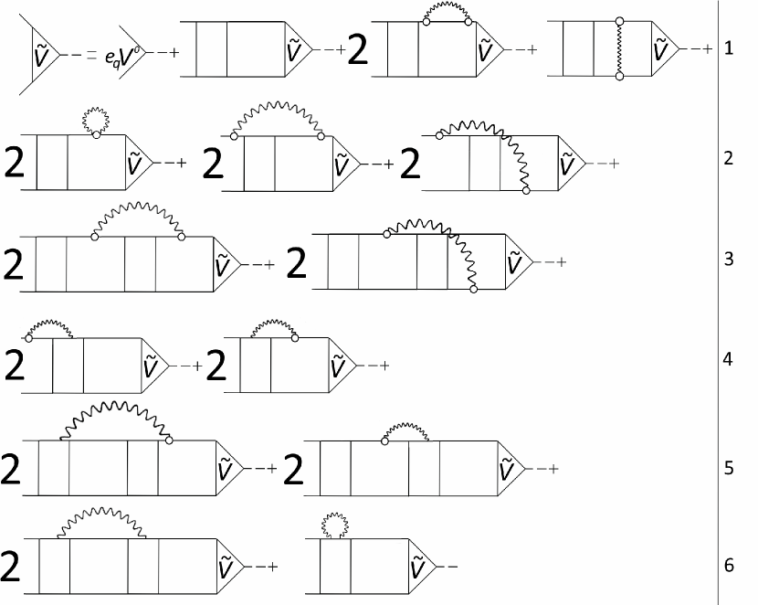
Figure 6: Equation (16) for the new effective field $\tilde{V}$ with PC in the diagrammatic representation. For convenience, numeration on the right gives numbers of the lines here and in Eq.(16)

IV Discussion of the equation for the new effective field $\tilde{V}$

For simplicity, we enumerate the terms of Eq. (16),Fig.6, in accordance with their lines as follows:

$$\tilde{V}=\tilde{V}^{1}+\tilde{V}^{tad}+\tilde{V}^{2}+\tilde{V}^{3}+\tilde{V}^{4}+\tilde{V}^{5}+\tilde{V}^{6}$$ (17)

Here the upper indices mean only the number of the line in Eq. (16),Fig.6. The separate parts of Eq.(17) may include two or three terms in each line.

1. The first term, $\tilde{V}^{1}$, corresponds to previous approaches kaev83 ; ts89 ; Tselyev2016 , which use the ph- propagator with PC shown in Fig.1. For the completeness, we give the term of $\tilde{V}^{1}$, which contains the second part of $\tilde{V}^{1}$ (with insertions). The third part (with the old induced interaction) will be discussed in section B. See also Ref.revKST for detailed discussions of the TBA approaches.

$$\tilde{V}^{1(2)}=\sum_{3465,s}F_{1263}g_{34}g_{45}\tilde{V}_{56}I_{3456,s}^{(1)}(\omega)$$ (18)

where

$$I_{3456,s}^{(1)}(\omega)\!\!=\!\!\!\!\int\!\!\!G_{3}(\varepsilon)G_{5}(\varepsilon)G_{6}(\varepsilon-\omega)\times$$

$$G_{4}(\varepsilon-\omega_{1})D_{s}(\omega_{1})d\varepsilon d\omega_{1}$$

$$=\frac{1}{(\varepsilon_{63}+\omega)\varepsilon_{53}}\cdot\Biggl{(}\frac{n_{6}(1-n_{4})}{\varepsilon_{46}+\omega_{s}-\omega}-\frac{n_{4}(1-n_{6})}{\varepsilon_{46}-\omega_{s}-\omega}+$$

$$\frac{n_{4}(1-n_{3})}{\varepsilon_{43}-\omega_{s}}-\frac{n_{3}(1-n_{4})}{\varepsilon_{43}+\omega_{s}}\Biggr{)}-$$

$$-\frac{1}{(\varepsilon_{65}+\omega)\varepsilon_{53}}\cdot\Biggl{(}\frac{n_{6}(1-n_{4})}{\varepsilon_{46}+\omega_{s}-\omega}-\frac{n_{4}(1-n_{6})}{\varepsilon_{46}-\omega_{s}-\omega}+$$

$$\frac{n_{4}(1-n_{5})}{\varepsilon_{45}-\omega_{s}}-\frac{n_{5}(1-n_{4})}{\varepsilon_{45}+\omega_{s}}\Biggr{)}$$ (19)

Hereinafter $\varepsilon_{34}=\varepsilon_{\lambda_{3}}-\varepsilon_{\lambda_{4}},n_{3}=n_{\lambda_{3}}$, the low indices mean the set 1$\equiv({n_{1},j_{1},l_{1},m_{1}})$, and we write down only one term of Eq.(16),Fig.6, which contains number 2.

Below we discuss the new terms of Eq.(16), Fig.6.

2. In the second lines of Eq.(16),Fig.6, we obtained the tadpole contribution $\tilde{V}^{tad}$ and four graphs with the general structure which is similar to the PC graphs of the first line in the sense that all of them contain four GFs G, one phonon GF D and two phonon creation amplitudes $g$.

3. In the third line, there are rather complex graphs with two effective interactions F, six GFs G, one phonon GF D and two phonon creation amplitudes $g$.

All the 4-th, 5-th and 6-th lines contain the variations of the effective interaction $\delta F$ of the first and second orders:

4. In the fourth line, rather simple graphs with three GFs G , one phonon GF D and one phonon creation amplitude $g$ are present.

5. In the fifth line, we have rather complex graphs which contain simultaneously the effective interaction F, its variations $\delta F$ and one phonon creation amplitude $g$.

6. Finally, in the last, sixth line, there are one GF D, two first order variations of the effective interaction $F$, four GFs G (the first graph) and the second order variation of $F$ $\delta^{(2)}F$ with two GFs G and one GF D(the second graph).

IV.1 The term with tadpole

Let us discuss the term in the second line of Eq.(16),Fig.6 ($\tilde{V}^{tad}$ of Eg. (17)). One can see, it has a relatively simple structure:

$$\tilde{V}^{tad}_{12}=\Sigma F_{1234}\tilde{V}_{54}K^{ph}_{35}I_{354}(\omega)$$ (20)

$$I_{354}(\omega)=\int G_{3}(\varepsilon)G_{5}(\varepsilon)G_{4}(\varepsilon-\omega)d\varepsilon=$$

$$\frac{n_{3}-n_{4}}{(\varepsilon_{34}-\omega)(\varepsilon_{54}+\omega)}+(1-\delta_{35})\frac{n_{3}-n_{5}}{\varepsilon_{35}(\varepsilon_{54}+\omega)}$$ (21)

In the works of the Kurchatov institute group, it was shown that, as a rule, the quantitative tadpole contributions to characteristics of the ground and low-lying states are rather considerable and have the opposite sign as compared to the pole (usual) diagrams. One can think that tadpole term $\tilde{V}^{tad}_{12}$ should give the same effect as compared to the insertion terms in $\tilde{V}^{1}$ of Eq.(17).

IV.2 Terms $\tilde{V}^{2}$ with new induced interactions

As one can see from Fig.6, the term $\tilde{V}^{2}$ of Eq.(17) contains two new induced interactions caused by the exchange of our phonon in the second ph-channel and in the particle-particle channels. We call these new terms of $\tilde{V}^{2}$ as $\tilde{V}^{ph2}$ and $\tilde{V}^{pp}$ because the term in $\tilde{V}^{1}$ with the old induced interaction (caused by the exchange of the same ph-phonon) can be called as $\tilde{V}^{ph1}$ and is already contained in the last term of the first line of Fig.6. All of them are shown in Fig.7: the old one $\tilde{V}^{ph1}_{12}$ and two new ones $\tilde{V}^{ph2}_{12}$ and $\tilde{V}^{pp}_{12}$. Each of the induced interactions, by our definition, contains the effective interaction $F$, two single-particle GFs G , one phonon GF D , two phonon creation amplitudes $g$ and depends on the single-particle energy variable $\varepsilon_{1}$. This dependence corresponds to the time variable of particle 1 in the $\delta$-function $\delta(\varepsilon_{1}-\varepsilon_{2}-\omega)$, which always appears in all final formulas for $\tilde{V}$.

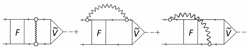
Figure 7: Terms of Eq.(16),Fig.6 with induced interactions:the old one $\tilde{V}^{ph1}_{12}$ and new $\tilde{V}^{ph2}_{12}$ and $\tilde{V}^{pp}_{12}$.

The old term $\tilde{V}^{ph1}_{12}$, which is contained in the term $\tilde{V}^{1}$ of Eq.(17), is as follows:

$$\tilde{V}^{ph1}_{12}=\sum_{3465,s}F_{1243}g_{35}g_{65}\tilde{V}_{56}I_{3456,s}^{(2)}(\omega)$$ (22)

where

$$I_{3456,s}^{(2)}(\omega)\!\!=\!\!\!\!\int\!\!\!G_{3}(\varepsilon)G_{6}(\varepsilon-\omega)D_{s}(\omega_{1})\times$$

$$G_{4}(\varepsilon-\omega_{1})G_{5}(\varepsilon-\omega_{1}-\omega)d\varepsilon d\omega_{1}$$

$$=\frac{1}{(\varepsilon_{63}+\omega)(\varepsilon_{45}-\omega)}\cdot\Biggl{(}\frac{n_{6}(1-n_{4})}{\varepsilon_{46}+\omega_{s}-\omega}-\frac{n_{4}(1-n_{6})}{\varepsilon_{46}-\omega_{s}-\omega}+$$

$$\frac{n_{5}(1-n_{3})}{\varepsilon_{35}+\omega_{s}-\omega}-\frac{n_{3}(1-n_{5})}{\varepsilon_{46}-\omega_{s}-\omega}+\frac{n_{6}(1-n_{5})}{\varepsilon_{65}-\omega_{s}}-$$

$$\frac{n_{5}(1-n_{6})}{\varepsilon_{65}+\omega_{s}}+\frac{n_{4}(1-n_{3})}{\varepsilon_{43}-\omega_{s}}-\frac{n_{3}(1-n_{4})}{\varepsilon_{43}+\omega_{s}}\Biggr{)}$$ (23)

We have applied the simple and useful formula:

$$G_{\lambda}(\varepsilon)\cdot G_{\lambda^{\prime}}(\varepsilon+\omega)=\frac{G_{\lambda}(\varepsilon)-G_{\lambda^{\prime}}(\varepsilon+\omega)}{\varepsilon_{\lambda}-\varepsilon_{\lambda^{\prime}}+\omega}$$ (24)

In the microscopic theory of GMR, it is well known that , as a rule, the term $\tilde{V}^{ph1}_{12}$ has the opposite sign as compared to insertion terms in $\tilde{V}^{1}$ and the maximal cancellation is for E0 resonances. In the previous section A, it was said that the quantitative contribution of tadpole terms has the opposite sign as compared to contributions of pole diagrams. By analogy, one can think that the relative role of $\tilde{V}^{ph1}_{12}$ should be increased as compared to insertion terms in $\tilde{V}^{1}$. Thus, the quantitative final contribution of our new tadpole terms may be of great interest.

$\tilde{V}^{ph1}_{12}$ does not depend on the energy variable, while the new terms $\tilde{V}^{ph2}_{12}$ and $\tilde{V}^{pp}_{12}$ depend on the energy variable $\varepsilon_{1}$:

$$\tilde{V}^{2}_{12}(\varepsilon_{1},\omega)=\tilde{V}^{ph2}_{12}(\varepsilon_{1},\omega)+\tilde{V}^{pp}_{12}(\varepsilon_{1},\omega),$$ (25)

$$\tilde{V}^{ph2}_{12}(\varepsilon_{1},\omega)=\sum_{3465,s}g_{13}g_{46}F_{3254}\tilde{V}_{65}I^{(1)}_{3465,s}(\varepsilon_{1},\omega),$$ (26)

$$\tilde{V}^{pp}_{12}(\varepsilon_{1},\omega)=\sum_{3465,s}g_{13}g_{65}F_{3254}\tilde{V}_{46}I^{(2)}_{3465,s}(\varepsilon_{1},\omega).$$ (27)

where

$$I^{(1)}_{3465,s}(\varepsilon_{1},\omega)=\!\!\int\!I_{465}(\omega_{1},\omega)G_{3}(\varepsilon_{1},-\omega_{1})D_{s}(\omega_{1})d\omega_{1}$$ (28)

$$I^{(2)}_{3465,s}(\varepsilon_{1},\omega)\!=\!\!\!\int\!\!\!I_{465}(\!-\omega,\!-\omega_{1})G_{3}(\varepsilon_{1},\!-\omega_{1})D_{s}(\omega_{1})d\omega_{1}$$ (29)

$$I_{465}(\omega_{1},\omega)=\int G_{6}(\varepsilon)G_{5}(\varepsilon-\omega)G_{4}(\varepsilon-\omega_{1})d\varepsilon=$$

$$\frac{1}{\varepsilon_{54}+\omega_{1}-\omega}\cdot\Biggl{[}\frac{n_{6}-n_{5}}{\varepsilon_{65}+\omega}-\frac{n_{6}-n_{4}}{\varepsilon_{64}+\omega_{1}}\Biggr{]}$$ (30)

As one can see from Eqs.(22),(26),(27), each of the the quantities $\tilde{V}^{ph1},\tilde{V}^{ph2},\tilde{V}^{pp}$ has the similar structure: the effective interaction $F$, vertex $\tilde{V}$, two amplitudes of phonon creation $g$, four single-particle GFs G and one phonon GF D. At this stage, one can not see a noticeable quantitative difference between them, but, of course, only calculations should clarify this statement. The difference of the similar quantity $\tilde{V}^{4(1)}$, Eq.(34) (see below) from the above-mentioned ones is that $\tilde{V}^{4(1)}$ contains $\delta F$ instead of $F$ and this difference may be noticeable. The quantities $\tilde{V}^{ph2},\tilde{V}^{pp}$ and $\tilde{V}^{4(1)}$ contain an unexpected effect - they depend on the energy variable $\varepsilon_{1}$. Physically, it is not difficult to understand: after the very first interaction of the external field with a nucleus, one of the quasiparticles of the initial ph-pair may create not the next ph-pair, as in the usual RPA, but a phonon with the creation amplitude $g$, and after that another ph-pair may interact with other ones through effective interaction. In other words, our approach gives more than earlier, additional possibilities to create the complex configurations 1p1h$\otimes$phonon and this can be clearly seen in Fig.6.

The dependence of the effective field (vertex) on the energy variable $\varepsilon_{1}$ arose for the first time. It is caused by the first term of Eq.(9). Note that this term of Eq.(9) gives in sum eight terms in Fig.6 (connected with $\delta(1)\tilde{V}$ in Eq.(9)), including three ”dangerous” terms with the induced interactions under consideration.

Such a dependence of the vertex on the energy variable $\varepsilon_{1}$ (or time in the time representation) is quite new and it should be investigated in the future. At present, one can say the following. Our vertex $\tilde{V}$ is , by definition, a change of FG G in the weak external field $V^{0}$ and the $\varepsilon_{1}$ dependence arose from the account for PC for the vertex. There is an analogy with $\varepsilon$-dependence and PC role in the optical potential $V_{opt}$, which is, in fact, mass operator $\Sigma(\varepsilon)$, for example, see article Giai . By analogy, one can speak about $Re\tilde{V}$ and $Im\tilde{V}$. Then $Im\tilde{V}$ corresponds to a change of an absorption in the external field, i.e. to the quantity $ImV_{opt}$. As the microscopic calculations Giai of PC contribution to $V_{opt}$ showed, the addition of PC to $ImV_{opt}$ turned out too insignificant to explain the experiment. Maybe, one can hope that such analogy may justify the suggestion that in the calculations for the beginning one can use the approximation $\varepsilon_{1}=\varepsilon_{\lambda_{1}}$, where $\varepsilon_{\lambda_{1}}$ is the single-particle energy, i.e. to take $\varepsilon_{1}$ on the mass surface.

IV.3 Terms in the third line of Eq.(16),Fig.6

The next terms of the third line of Eq.(16),Fig.6 can be expressed through $\tilde{V}^{ph2}_{12}$ and $\tilde{V}^{pp}_{12}$:

$$\tilde{V}^{3}_{78}= \sum_{21}F_{7821}\int G_{1}(\varepsilon)G_{2}(\varepsilon-\omega)(\tilde{V}^{ph2}_{12}+\tilde{V}^{pp}_{12})(\varepsilon,\omega)d\varepsilon$$

$$= \sum_{213465,s}F_{7821}g_{13}g_{46}F_{3254}V_{65}I^{ph2}_{213465,s}+$$

$$\sum_{213465,s}F_{7821}g_{13}g_{65}F_{3254}\tilde{V}_{46}I^{pp}_{213465,s}$$ (31)

where

$$I^{ph2}_{213465,s}=\int G_{1}(\varepsilon)G_{2}(\varepsilon-\omega)I^{(1)}_{3465,s}(\varepsilon,\omega)d\varepsilon$$ (32)

$$I^{pp}_{213465,s}=\int G_{1}(\varepsilon)G_{2}(\varepsilon-\omega)I^{(2)}_{3465,s}(\varepsilon,\omega)d\varepsilon$$ (33)

with $I^{(1)}_{3465,s}(\varepsilon,\omega)$ and $I^{(2)}_{3465,s}(\varepsilon,\omega)$ from Eq.(28) and Eq.(29)

IV.4 Terms containing $\delta F$

IV.4.1 Terms in the fourth line of Eq.(16),Fig.6

The first term $\tilde{V}^{4(1)}$ of $\tilde{V}^{4}$:

$$\tilde{V}^{4(1)}_{12}(\varepsilon)=\sum_{345,s}g_{13}\delta F_{3254,s}V_{45}I^{(1)}_{345,s}(\varepsilon,\omega)$$ (34)

$$I^{(1)}_{345,s}(\varepsilon,\omega)=A_{45}(\omega)I_{3,s}(\varepsilon),$$

$$I_{3,s}(\varepsilon)=\int G_{3}(\varepsilon-\omega_{1})D_{s}(\omega_{1})d\omega_{1}=$$

$$\frac{n_{3}}{\varepsilon+\omega_{s}-\varepsilon_{3}-i\gamma}+\frac{1-n_{3}}{\varepsilon-\omega_{s}-\varepsilon_{3}+i\gamma}$$ (35)

Again, we get here the dependence on the energy variable $\varepsilon$ caused by the first term of Eq.(9), see the discussion in section B.

The second term $\tilde{V}^{4(2)}$ is as follows

$$\tilde{V}^{4(2)}_{12}=\sum_{345,s}\delta F_{1254,s}g_{34}V_{45}I^{(2)}_{345,s}(\omega)$$ (36)

$$I^{(2)}_{345,s}(\omega)=\int G_{3}(\varepsilon-\omega_{1})G_{4}(\varepsilon)G_{5}(\varepsilon-\omega)D_{s}(\omega_{1})d\varepsilon d\omega_{1}=$$

$$\!=\frac{1}{\varepsilon_{45}+\omega}\!\!\int\!\!\biggl{(}G_{4}(\varepsilon)-G_{5}(\varepsilon)\biggr{)}\!\!\!\times\!\!G_{3}(\varepsilon-\omega_{1})D_{s}(\omega_{1})d\varepsilon d\omega_{1}=$$

$$\frac{1}{\varepsilon_{45}+\omega}\int\biggl{(}G_{4}(\varepsilon)-G_{5}(\varepsilon)\biggr{)}I_{3s}(\varepsilon)d\varepsilon$$ (37)

with $I_{3s}(\varepsilon)$ from Eq.(35)

Thus, for $I^{(2)}_{345,s}$ we have:

$$I^{(2)}_{345,s}(\omega)=\frac{1}{\varepsilon_{45}+\omega}\Biggl{[}\frac{n_{4}(1-n_{3})}{\varepsilon_{43}-\omega_{s}}-\frac{(1-n_{4})n_{3}}{\varepsilon_{43}+\omega_{s}}+$$

$$\frac{n_{5}(1-n_{3})}{\varepsilon_{53}-\omega_{s}+\omega}-\frac{(1-n_{5})n_{3}}{\varepsilon_{53}+\omega_{s}+\omega}\Biggr{]}$$ (38)

IV.4.2 Terms in the fifth line of Eq.(16),Fig.6

These terms contain $\delta F$ and $F$

$$\tilde{V}^{5(1)}_{12}(\omega)=\sum_{34657,s}\delta F_{1234,s}F_{3457}g_{76}V_{65}I_{34765,s}(\omega)$$ (39)

$$I_{34765,s}(\omega)=\int A_{34}(\omega-\omega_{1})I_{765}(\omega,\omega_{1})D_{s}(\omega_{1})d\omega_{1}$$ (40)

with $I_{765}(\omega,\omega_{1})$ from Eq.(30)

The second term of $\tilde{V}^{5(2)}$ is:

$$\tilde{V}^{5(2)}_{12}(\omega)\!\!=\!\!\sum_{3456,s}\!\!F_{1234}\!\int\!G_{3}(\varepsilon)G_{4}(\varepsilon-\omega)V_{34}^{4(1)}(\varepsilon-\omega)d\varepsilon$$ (41)

with $V_{34}^{4(1)}(\varepsilon-\omega)$ from Eq.(34)

IV.4.3 The first term in the sixth line of Eq.(16),Fig.6

Here we have

$$\tilde{V}^{6(1)}_{12}(\omega)=\sum_{3456,s}\delta F_{1243,s}\delta F_{3465,s}V_{56}I_{3456,s}(\omega),$$

$$I_{3456,s}(\omega)=A_{56}(\omega)\cdot\int A_{34}(\omega,-\omega_{1})D_{s}(\omega_{1})d\omega_{1}$$ (42)

IV.5 Term containing $\delta^{(2)}F$

The second term of $\tilde{V}^{6}$:

$$\tilde{V}^{6(2)}_{12}(\omega)=\sum_{54}\delta^{(2)}F_{3254}DV_{45}A_{45}(\omega),$$ (43)

where $\delta^{(2)}F_{3254}$ should be obtained with a generalization of Eq.(6).

V Energies and probabilities of transitions

Below we describe, in a short form, a general scheme for calculations of the observable characteristics within our approach. It may be also useful for calculations and analysis of selected terms of Eq.(16),Fig.6. In order to see more clearly the main features of the method, Eq.(16),Fig.6 can be written in the following form:

$$\tilde{V}=e_{q}V^{0}+FA^{1}\tilde{V}+F(A^{tad}+A^{2}+A^{3})\tilde{V}+$$

$$\delta F(A^{4}+A^{5})\tilde{V}+(\delta F)^{2}A^{6(1)}\tilde{V}+\delta^{(2)}FA\tilde{V}$$ (44)

with the obvious notations for the propagators $A^{i}$, for which the indices $i$ correspond to the numbers of lines in Eq.(16),Fig.6 and parts $V^{i}$ in Eq.(17). Here $A^{1}$ corresponds to the previous approach kaev83 ; ts89 and (without pairing) ts2007 , which includes the RPA part and PC part with two graphs with insertions and induced interaction $F^{ph1}$ shown in Fig.1 Propagators $A^{i}$ can be easily obtained: $A^{1}$ from Eqs.(18),(22), $A^{tad}$ from Eq.(20), $A^{2}$ from Eqs.(26),(27), $A^{3}$ from Eq.(31),$A^{4}$ from Eqs.(34),(36), $A^{5}$ from Eqs.(39),(41), $A^{6(1)}$ from Eq.(42). The quantity $A^{5}$ contains the effective interaction $F$.

To get formulas for energies and probabilities of transitions between the ground and excited states, we generalise the method of standard TFFS Migdal . In the pole under consideration $\omega=\omega_{n}$, the vertex $\tilde{V}$ has a form

$$\tilde{V}=\frac{\chi^{n}}{\omega-\omega_{n}}+\tilde{V}^{R},$$ (45)

where $\omega_{n}$ is the energy of the excited state under consideration, $\chi^{n}$ is the residue in this pole and $\chi^{R}$ is a regular part of $\tilde{V}$. Then the transition energies should be found from the homogeneous equation

$$\chi^{n}=FA^{1}\chi^{n}+F(A^{tad}+A^{2}+A^{3})\chi^{n}+$$

$$\delta F(A^{4}+A^{5})\chi^{n}+(\delta F)^{2}A^{6(1)}\chi^{n}+\delta^{(2)}FA\chi^{n}$$ (46)

It is convenient to rewrite Eq.(44) in a more compact form:

$$\tilde{V}=e_{q}V^{0}+F\overline{A}\tilde{V}.$$ (47)

where $\overline{A}$ has a complicated form and can be obtained from Eq.(44). It depends on four single-particle indices , can contain the effective interaction $F$, $\delta F$ and different sums. Then, the transition energies should be found from the homogeneous equation:

$$\chi^{n}=F\overline{A}^{n}\chi^{n},$$ (48)

where $\overline{A}^{n}=\overline{A}(\omega=\omega_{n})$

In order to find a normalization condition for the residue $\chi^{n}$, first, we derive the equation for $\tilde{V}^{R}$:

$$\tilde{V}^{R}=e_{q}V^{0}+F\overline{A}^{n}\tilde{V}^{R}+F\frac{d\overline{A}^{n}}{d\omega}\chi^{n}$$ (49)

and multiply it on the left by $\chi^{n}\overline{A}^{n}$. As a result, we obtain the normalization condition for the residue $\chi^{n}$:

$$\chi^{n}\overline{A}^{n}e_{q}V^{0}=-\chi^{n}\frac{d\overline{A}^{n}}{d\omega}\chi^{n}.$$ (50)

Let us obtain the probabilities of transitions between the ground and excited states. This quantity is defined as usual:

$$W_{0n}=2\pi\mid M_{0n}\mid^{2}\delta(\omega-\omega_{n})$$ (51)

where the matrix element should be found from the polarizability operator, which contains the change of the density matrix $\rho$ in the external field for the transition from the ground to excited state $n$:

$$\Pi(\omega)=\sum_{12}V^{0}_{12}\rho_{21}.$$ (52)

Further, it is quite natural to define our density matrix $\rho$ in the following form:

$$\rho=\overline{A}\tilde{V}$$ (53)

One can show that this definition is the same, within our $g^{2}$ approximation, as the usual definition $\rho=\int GG\tilde{V}d\epsilon$. So, from Eq.(47) we have the equation for $\rho$:

$$\rho=\overline{A}e_{q}V^{0}+\overline{A}F\rho$$ (54)

The transition probabilities should be obtained as the residue of the polarizability operator

$$W_{0n}=2Im(e_{q}V^{0}\rho)^{n}$$ (55)

with the residue $\eta^{n}$ of $\rho$ in the pole $\omega_{n}$

$$\rho=\frac{\eta^{n}}{\omega-\omega_{n}}+\rho^{R},$$ (56)

so that from Eq.(45) we have

$$\rho=\overline{A}(\frac{\chi^{n}}{\omega-\omega_{n}}+V^{R})$$ (57)

and for the residue $\eta^{n}$ we find

$$\eta^{n}=\overline{A}\chi^{n}$$ (58)

Finally, we obtain :

$$W_{0n}=(e_{q}V^{0}\overline{A}\chi^{n})$$ (59)

or, accounting for the normalization condition Eq.(50):

$$W_{0n}=\frac{(e_{q}V^{0}\overline{A}\chi^{n})^{2}}{(-\chi^{n}\frac{d\overline{A}}{d\omega}\chi^{n})}$$ (60)

For the energy regions, for which it is not possible to study the individual eigenenergies of the states, it is necessary to have an envelope of GMR under consideration. Then it makes sense to use the smearing parameter $\Delta$, which greatly reduces numerical difficulties of the calculations, if, of course, a peaked function has a width substantially larger than the energy averaging interval, see revKST . In this case one uses the strength function

$$S(\omega,\Delta)=\frac{dB(EL)}{d\omega}=-\frac{1}{\pi}Im\sum_{12}e_{q}V^{0}_{12}\rho_{21}(\omega+\imath\Delta),$$ (61)

from which one can easily obtain the transition probabilities and energy-weighed sum rule, summed over an energy interval.

The formulas obtained in this section are very general and can be also used, if necessary, to study any selected part of Eq.(17) or Eq.(47).

VI Conclusion

In this work, the formalism of many-body nuclear self-consistent theory, the quantum GF method, to be exact, has been applied for PDR and GMR in magic nuclei to take PC effects and complex 1p1h$\otimes$phonon configurations into account. The main physical difference from the previous approaches is that, due to consistent inclusion of PC effects, our approach gives much more than earlier additional possibilities to create the complex configurations 1p1h$\otimes$phonon and that can be cleary seen from Fig.6. It is necessary to note that within the method under consideration, one can take into account the single-particle spectrum revKST and, which is more important, all the new (as compared to the case of RPA ) numerous ground state correlations (GSC), including three-quasiparticle GSC , for example, in $\tilde{V}^{tad}$ of Eq.(17), and more complex GSC. The effects of new three- and four-quasiparticle GSC were disscused in voitenkov ; picma for the case of ground and low-lying states and, as it turned out, they are very considerable.

A new equation for the effective field with PC and quite new PC contributions to the effective field, which are of interest in the energy regions of PDR and GMR, have been obtained. These contributions are: i)the tadpole effect in the standard ph-propagator, ii)two new induced interactions due to phonon exchange in the second ph-channel (in addition to the old induced interaction in the first ph-channel ) and the induced interactions in the pp- and hh-channels, iii) the effects of the first and second variations of the effective interaction in the phonon field.

Thus, we have extended the above-mentioned self-consistent approach KhSap1982 to the energy region of PDR and GMR in order to describe on the equal footing both the ground states and all the region of nuclear excitations up to GMR energies (30-35 MeV). This extension does not concern only the PDR and MGR energy region, but also generalizes the TFFS formalism. In this sense, one can speak about the beginning of the third stage of developing TFFS. As it was mentioned in the Introduction, and we would like to stress it again that, if necessary, the prescription of MCDD, or TBA ts89 should be used in calculations. Unfortunately, at present there is no other method to solve the second order poles problem within the formalism considered.

We have considered, rather schematically, all the terms in the new equation for the effective field $\tilde{V}$ Eq.(16),Fig.6. Strictly speaking, at the present stage it is not possible to speak about numerical contributions of the separate terms in view of the fact that the approach is applicable for many physical cases (the multipole orders, energies of transitions, of excitations etc.). One can think, however, that the effects of the tadpole in the part $\tilde{V}^{tad}$ and of the new induced interactions in the parts $\tilde{V}^{2}$ and maybe (with $\delta F$) in $\tilde{V}^{4}$ can give something quite new both in qualitative and quantitative sense, while other terms with $\delta F$ and the term $\delta^{(2)}F$ can be not so important.

Probably, our new effects are of the highest interest for calculations of fine structures of GMR and, especially, PDR and other pygmy-resonances. As it was said in the Introduction, there are new physical phenomena in the PDR energy region and new experimental methods for fine structure studies, but there is no reasonable self-consistent explanation of the PDR fine structure even for ²⁰⁸Pb. However, the problem of the self-consistent explanation of GMR is topical too, first of all, for M1 resonances, where the problem with the second order poles are not so important ktZPhys . All these problems will be discussed by us in the future.

VII ACKNOWLEDGMENTS

We are grateful to V.A. Khodel ,S.V.Tolokonnikov and V.I. Tselayev for useful discussions and to S.S. Pankratov for discussions of calculation problems. The reported study was funded by RFBR, project no.19-31-90186 and supported by the Russian Science Foundation, project no.16-12-10155.

References

- (1) N. Paar, D. Vretenar, E. Khan, G. Colo, Rep. Prog. Phys. 70, 691 (2007).
- (2) A. Bracco, E.G. Lanza, and A. Tamii, Prog. Part. Nucl.Phys. 106, 360 (2019).
- (3) S.P. Kamerdzhiev, O.I. Achakovskiy, S.V. Tolokonnikov, M.I. Shitov, Phys. At. Nucl. 82, 366 (2019)
- (4) S. Kamerdzhiev, J. Speth, G. Tertychny, Phys. Rep. 393, 1 (2004).
- (5) A. Avdeenkov, S. Goriely, S. Kamerdzhiev, S. Krewald, Phys. Rev. C 83, 064316 (2011).
- (6) S. Goriely, E. Khan, V. Samyn, Nucl. Phys. A 739, 331 (2004).
- (7) S.P. Kamerdzhiev, A.V. Avdeenkov, D.A.Voitenkov, Phys. At. Nucl. 74, 1478 (2011).
- (8) V. Tselyaev, N. Lyutorovich, J. Speth, S. Krewald, and P.-G. Reinhard, Phys. Rev. C 94, 034306 (2016).
- (9) N. A. Lyutorovich, V. I. Tselyaev, O. I. Achakovskiy, and S. P. Kamerdzhiev, JETP Lett. 107, 659 (2018).
- (10) A. Repko, V.O. Nesterenko, J. Kvasil, and P.-G. Reinhard, arXiv:1903.01348 [nucl-th] (2019).
- (11) A. Tamii, I. Poltoratska, P. von Neumann-Cosel, Y. Fujita, T. Adachi, C. A. Bertulani, J. Carter, M. Dozono, H. Fujita, K. Fujita, K. Hatanaka, D. Ishikawa, M. Itoh, T. Kawabata, Y. Kalmykov, A. M. Krumbholz, E. Litvinova, H. Matsubara, K. Nakanishi, R. Neveling, H. Okamura, H. J. Ong, B. Özel-Tashenov, V. Yu. Ponomarev, A. Richter, B. Rubio, H. Sakaguchi, Y. Sakemi, Y. Sasamoto, Y. Shimbara, Y. Shimizu, F. D. Smit, T. Suzuki, Y. Tameshige, J. Wambach, R. Yamada, M. Yosoi, and J. Zenihiro, Phys. Rev. Let. 107, 062502 (2011).
- (12) A. C. Larsen, J. E. Midtbø, M. Guttormsen, T. Renstrøm, S. N. Liddick, A. Spyrou, S. Karampagia, B. A. Brown, O. Achakovskiy, S. Kamerdzhiev, D. L. Bleuel, A. Couture, L. Crespo Campo, B. P. Crider, A. C. Dombos, R. Lewis, S. Mosby, F. Naqvi, G. Perdikakis, C. J. Prokop, S. J. Quinn, and S. Siem, Phys. Rev. C 97, 054329 (2018).
- (13) E. E. Saperstein and S. V. Tolokonnikov, Yad.Fiz. 79, 703 (2016) [Phys. At.Nucl. 79, 1030 (2016)].
- (14) V. A. Khodel and E. E. Saperstein, Phys. Rep. 92,183 (1982).
- (15) A.V. Smirnov, S.V. Tolokonnikov, S.A. Fayans Sov. J. Nucl. Phys. 48, 995(1988).
- (16) D.Voitenkov, S. Kamerdzhiev, S. Krewald, E.E. Saperstein, S.V. Tolokonnikov, Phys. Rev. C 85, 054319 (2012).
- (17) A. B.Migdal, Theory of Finite Fermi Systems and Applications to Atomic Nuclei (Nauka, Moscow, 1965; Intersci., New York, 1967).
- (18) S.P. Kamerdzhiev, Yad. Fiz. 38, 316 (1983) [Sov. J. Nucl. Phys. 38,188 (1989) ].
- (19) V. I. Tselyaev, Yad. Fiz. 50, 1252 (1989) [Sov. J. Nucl. Phys. 50, 780 (1989) ].
- (20) V. Tselyaev, Phys. Rev. C 75, 024306 (2007)
- (21) S. P. Kamerdzhiev and V.N. Tkachev, Z. Phys.A334, 19 (1989).
- (22) S.P. Kamerdzhiev, A.V. Avdeenkov, O.I. Achakovskiy, Phys. Atom. Nucl. 77, 1303 (2014).
- (23) V. Tselayev, N. Lyutorovich, J. Speth, P.-G.Reinhard, Phys.Rev. C 97, 044308 (2018)
- (24) V.G. Soloviev, Theory of atomic nuclei: quasi-particles and phonons (Institute of physics, Bristol and Philadelphia, USA, 1992).
- (25) Nguyen Van Giai, Ch. Stoyanov, and V. V. Voronov, Phys. Rev. C 57, 1204 (1998).
- (26) V. A. Khodel, A.P. Platonov, E.E. Saperstein, J. Phys. G: Nucl. Phys. 6 1199 (1980).
- (27) E. E. Saperstein, O. I.Achakovskiy, S. P. Kamerdzhiev, S. Krewald, J.Speth, and S. V. Tolokonnikov, Physics of At. Nuclei, 77, 1033 (2014).
- (28) E.E. Saperstein, S.P. Kamerdzhiev, D. S. Krepish, S. V. Tolokonnikov and D. Voitenkov, J. Phys. G: Nucl. Part. Phys. 44, 065104 (2017).
- (29) V. Bernard and Nguyen Van Giai, Nucl. Phys. A327 397, (1979)
- (30) S.P. Kamerdzhiev, D.A.Voitenkov, E.E. Saperstain, S.V. Tolokonnikov, M.I. Shitov, JETP Lett, 106, No.3, 139 (2017).