Observation of plaquette fluctuations in the spin-1/2 honeycomb lattice

Abstract

Quantum spin liquids are materials that feature quantum entangled spin correlations and avoid magnetic long-range order at T = 0 K. Particularly interesting are two-dimensional honeycomb spin lattices where a plethora of exotic quantum spin liquids have been predicted. Here, we experimentally study an effective S = 1/2 Heisenberg honeycomb lattice with competing nearest and next-nearest neighbor interactions. We demonstrate that YbBr₃ avoids order down to at least T = 100 mK and features a dynamic spin-spin correlation function with broad continuum scattering typical of quantum spin liquids near a quantum critical point. The continuum in the spin spectrum is consistent with plaquette type fluctuations predicted by theory. Our study is the experimental demonstration that strong quantum fluctuations can exist on the honeycomb lattice even in the absence of Kitaev-type interactions, and opens a new perspective on quantum spin liquids.

Introduction

Magnetism arises because of the quantum mechanical nature of the electron spin, yet for the understanding of many materials, particularly those used in today’s applications, a classical approach is sufficient. Materials with strong quantum fluctuations are rare, but attract significant research attention since they hold enormous potential for future technologies [1] that make use of the long-range entanglement for quantum communication [2, 3]. Fault-tolerant quantum computers are proposed to operate with anyon quasi-particles [2] which exist in a class of quantum spin liquids [4, 5].

Quantum spin liquids (QSL) are caused by quantum fluctuations which reduce the size of the ordered magnetic moment of static magnetic structures and can affect the dynamics of the spin excitations. This happens in the $S=1/2$ frustrated antiferromagnetic square lattice, with competing nearest and next-nearest neighbour interactions, $J_{1},J_{2}$, where the zone boundary spin-waves develop a dispersion due to the presence of quantum dimer-type fluctuations between nearest neighbors [6]. These fluctuations are similar to the resonant valence bond fluctuations predicted in the frustrated triangular lattice [7], which are believed to be relevant for high-temperature superconductors [8]. Frustration can be induced by competing interactions and depending on their relative strength, incommensurate magnetic phases, valence bond solids with periodic ordering of local quantum states, or QSLs with different symmetry are theoretically predicted [4, 10, 11, 12, 13, 14, 15, 16]. In particular, it is expected that frustration enforces a quantum phase transition at which fractionalization of magnons into deconfined spinons occurs [9].

It has been a challenge to identify and understand appropriate model systems to study QSLs. In general, lowering the dimension will increase quantum fluctuations. In one-dimension QSLs have been identified in antiferromagnetic (AF) spin chains. Case in point are KCuF₃ [17] and Cu(C₆D₅COO)${}_{2}\cdot$ 3D₂O [18]. In two- and three-dimensions, quantum fluctuations can be enhanced by frustration, and there are several routes to achieve this: The inherent geometrical frustration of kagome [19], triangular [20], spinel [21] and pyrochlore [22] lattices may prohibit long-range ordering at low temperatures. Another promising candidate is the honeycomb lattice which has received relatively little attention until Kitaev’s work [4] when it was realized that bond-dependent anisotropic interactions can stabilize a new form of QSL whose properties are known exactly. Representatives materials are $\alpha$-RuCl₃ [23], Li₂IrO₃ [24] and H₃LiIr₂O₆ [25] which show signatures of spin correlations due to quantum entanglement.

Quantum fluctuations are enhanced in the honeycomb lattice compared to the square lattice since the number of neighbours of each spin is lower, thus placing it closer to the quantum limit. When next-nearest neighbour frustrating exchange interactions are sufficiently large compared to the nearest neighbour exchange, theories predict a quantum phase transition from a Néel ground state into a quantum entangled state. However, there is no consensus on the nature of this ground state: Theories predict either a QSL [12, 13] or a plaquette valence bond crystal (pVBC) [14, 15, 16] with different magnetic excitations which include spinons [12], rotons [16] or plaquette fluctuations[26].

Here, we study the static and dynamic properties of the trihalide two-dimensional compound YbBr₃ that forms a realization of the undistorted S=1/2 honeycomb lattice with frustrated interactions. Short-range magnetic correlations between the Yb moments develop below $T\approx$ 3 K, but the correlation length is only of the order of the size of an elementary honeycomb plaquette at $T\leavevmode\nobreak\ =$ 100 mK, consistent with a QSL ground state. Despite this short correlation length, inelastic neutron measurements reveal well defined dispersive low energy magnetic excitations close to the Brillouin zone center. At high energies and at the zone boundary, we observe a continuum of excitations that we interpret as quantum fluctuations on an elementary hexagonal plaquette.

Results

Crystal structure and susceptibility

YbBr₃ crystallizes with the BiI₃ layer structure in the rhombohedral space group $R\bar{3}$ (148), where the Yb ions form perfect two-dimensional (2D) honeycomb lattices perpendicular to the $c$-axis, as shown in Fig. 1. The temperature dependence of the magnetic susceptibility has a broad maximum around $T=3\;\mathrm{K}$, but as shown below, there is no evidence for long-range magnetic order down to at least $T=100\;\mathrm{mK}$. In the low temperature regime below 10 K we observe $\rm\leavevmode\nobreak\ \chi^{a}\approx 1.3\chi^{c}$ which reflects a small easy-plane anisotropy.

The rare earth ion Yb³⁺ features a $J=7/2$ ground-state multiplet that is split by the crystal-electric field (CEF), giving rise to a total of four Kramers doublets with the three excited CEF levels being observable via neutron scattering. The first excited level is observed at $\sim 15$ meV and the ground-state doublet is an effective $S=1/2$ state. From an analysis of the measured susceptibility and the inelastic neutron data we obtain the CEF parameters (cf. Suppl. Info). They result in ground state expectation values of $\langle J_{\perp}\rangle=1.2$ and $\langle J_{\parallel}\rangle=0.8$ where the subscript indicates spin orientations measured relative to the $c$-axis.

Magnetic ground state

Fig. 2a shows the neutron diffraction pattern of the energy integrated magnetic scattering of Yb₃ that was determined as the difference between diffraction patterns taken at $T=100$ mK and $T=10$ K in order to eliminate the contributions of nuclear scattering. No magnetic Bragg peaks are visible in the diffraction pattern, demonstrating that $\rm\leavevmode\nobreak\ YbBr_{3}$ avoids magnetic order down to at least this temperature.

Diffuse magnetic scattering is centred at $(1,0,0)$ and equivalent wave-vectors, which implies that the short-range correlations are described by a propagation vector Q₀ = (0,0,0). Fig. 2b shows the diffuse scattering as obtained from the 2D spin wave theory described below, which reproduces both position and intensity of the observed diffuse scattering.

Fig. 2c shows a cut along the $\textbf{Q}=(q,0,0)$ direction which reveals diffuse scattering with Lorentzian line shape that reflects short-range magnetic order [27]. From a fit to the neutron intensity $I\propto\kappa^{2}/(q^{2}+\kappa^{2})$, we determine an in-plane correlation length between the Yb moments of $\xi=1/\kappa\approx 10\leavevmode\nobreak\ \rm\AA$ at $T=100$ mK, comparable to the fourth nearest-neighbour distance of $10.66\leavevmode\nobreak\ {\rm\AA}$ which is $\sim$1.25 times the diameter of an Yb₆-hexagon plaquette.

Magnetic excitations

We measured well-defined magnetic excitations at $T=250$ mK along three cuts in the hexagonal plane. Within experimental resolution we observed a single excitation branch and no spin gap at the zone centre. As shown in the constant energy-scans in Fig.  2d and in Fig. 3, the magnetic excitations are sharp close to the Brillouin zone center. One of the key results of this study is the observation of a broadening of the spectrum when the dispersion approaches the zone boundary, as shown in Fig. 3. In fact, the inelastic neutron spectrum close to the zone boundary exhibits a continuum which extends to over twice the energy of the well-defined magnetic excitation. While low-lying excitations are sharp, these broad excitations are only observed at higher energies.

While it may appear surprising that we observe well defined excitations even in the presence of a correlation length of merely 10 ${\rm\AA}$, this agrees with the predictions of Schwinger-Boson [28] and modified spin-wave [29] theories which show that spin-waves can propagate in low-dimensional systems with short-range Néel order. The well-defined excitations in YbBr₃ can be described by an effective $S=1/2$ Hamiltonian including nearest and next-nearest neighbour Heisenberg exchange coupling, and dipolar interactions between the CEF ground state doublets,

$$H=-\frac{1}{2}\sum_{i,j}\sum_{\alpha,\beta}{\cal J}_{\alpha,\beta}(i,j)S^{\alpha}_{i}S^{\beta}_{j},$$ (1)

where ${\cal J}_{\alpha,\beta}(i,j)=g^{2}_{\alpha}\delta_{\alpha\beta}J(i,j)+g_{\alpha}g_{\beta}D_{\alpha,\beta}(i,j)$, with $\alpha,\beta=x,y,z$ cartesian coordinates of the hexagonal cell, and $S^{\alpha}_{i}$ is the $\alpha$-component of a spin-1/2 operator at site $i$. Here $J(i,j)$, are the exchange coupling constants between distinct sites $i$ and $j$, while $D(i,j)$ denote the dipolar interactions. For the calculation of the spin wave dispersion, we use the random phase approximation (RPA) around the Néel state with spins in the hexagonal plane and $S=1/2$. Our measurements allow the determination of the exchange couplings, while the dipolar coupling is fixed by the magnetic moment. As shown in Fig. 3, we find good agreement between measured and calculated spin-wave dispersions. The nearest- and next-nearest-neighbour exchange interactions $J_{1}$, $J_{2}$ are obtained from a least-square fit to the data. We obtained $g^{2}J_{1}=-0.69(8)\,\rm{meV}$ and $g^{2}J_{2}=-0.09(2)\,{\rm meV}$ (see Suppl. Info. for details). We note that our spin wave theory does not describe all aspects of our experimental results: It predicts an optical branch for values of the easy-plane anisotropy that corresponds to the measured susceptibility (cf. Fig. 1), while we do not find experimental evidence for such a second branch. Also it does not explain the existence of an excitation continuum as we shall discuss next.

Continuum of excitations

As shown in Fig. 3, the magnetic excitation spectrum also features weaker broad scattering at energies where the optical branch is expected. This is particularly evident near the M-points at $(0.5,0.5,0)$ and $(0.5,-1,0)$, where the excitations extend to $0.8$ - $1\;\mathrm{meV}$ and are reminiscent of scattering observed in other low-dimensional antiferromagnets [31, 30]. In most materials, spin-waves are long-lived excitations that are resolution-limited as a function of energy. When the spin-waves are damped or interact with other spin-waves they have a finite life-time and the line-shape of the dynamical structure factor S(Q, $\omega$) broadens. We have simulated the line-shape of S(Q, $\omega$) derived from our model and convoluted it with the resolution of the spectrometer obtained from the Takin software [32] (cf. Methods). While the spin-wave model adequately explains the dispersion and intensity distribution close to the Brillouin zone centers, it does not reproduce the inelastic neutron line-shape close to the maximum of the dispersion of the spin-wave branch as shown in Fig. 4.

Discussion

The spin wave dispersion in YbBr₃ can be well described by a spin-1/2 Heisenberg Hamiltonian including nearest and next-nearest interactions with $J_{2}/J_{1}\approx 0.13$. This is close to the value $J_{2}/J_{1}\approx 0.16$ [10], where classical theories predict instability of the Néel state, and also close to $J_{2}/J_{1}\approx 0.1$ [11, 29], where quantum fluctuation in linear spin wave theory destroy long-range Néel order. We note that other theoretical approaches find that quantum fluctuations may stabilize the Néel phase up to somewhat higher ratios of $J_{2}/J_{1}$. These approaches include Schwinger boson approach [12], variational wave functions [33, 16] and exact diagonalization [14] which all yield a critical ratio $J_{2}/J_{1}\approx 0.2$. Since we do not find any evidence for static magnetism, we thus conclude that YbBr₃ must be in close proximity of such a quantum phase transition.

In YbBr₃ the Yb-ion has a large magnetic moment of the order of $2\,\mu_{B}$ and therefore the dipolar interactions cannot be neglected. At the classical level, one can show that they favour antiferromagnetic Néel order with the spins along the $c$-axis [34] enabled by a spin gap at the zone center of $\sim$ 200 $\mu$eV. This spin gap caused by the dipolar interaction is reduced by the CEF easy-plane anisotropy which contributes to a destabilization of the Néel state at finite temperature (Supplement Fig. S2). At $g_{\rm crit}\approx g_{zz}/g_{xx}\equiv$ 0.985 the spin gap closes and quantum fluctuations will be enhanced. Below that value the spins rotate into the basal plane. Linear spin wave theory predicts that easy-plane anisotropy entails a lifting of the degeneracy of the two spin-wave branches at the zone centre, and the splitting increases with increasing anisotropy. A large anisotropy in YbBr₃ would then become measurable since the branch separation becomes large enough to be resolved. A computation of S(Q, $\omega$) at $g_{\rm crit}$ is shown in Fig. 3 and describes the observed dispersion and intensities of the sharp excitations very well.

Experimentally, we have observed neither a splitting of spin waves nor a spin gap within the available energy resolution. This suggests that the absence of the long-range order in YbBr₃ at T = 100 mK is caused by the competition between easy-plane anisotropy and dipolar interactions that accentuates quantum fluctuations. This places YbBr₃ close to the quantum critical point towards a QSL of the spin-1/2 Heisenberg Hamiltonian on the honeycomb lattice.

Our experiment provides clear evidence for the presence of a continuum of excitations at high energies in YbBr₃. We can exclude the possibility of the line-shape broadening being caused by two-magnon decay. The necessary cubic anharmonicities are absent for collinear magnets such as YbBr₃ [35]. We observe that the intensity of the continuum is stronger at the M’ points along (h,-1,0) and (h,h,0) directions whereas it is absent along (0,k,0) and at the $\Gamma$ and $\Gamma^{\prime}{}$ points.

We found, as shown in Fig. 5, that this modulation of the neutron intensity associated with the continuum can be reproduced by a random-phase approximation (RPA) calculation for a hexamer plaquette with the exchange parameters obtained from the spin-wave calculations (cf. Methods). This picture of local excitations in YbBr₃ is supported by an analogous calculation of the magnetic susceptibility which shows a broad maximum at T $\simeq$ 4 K (see Supplement). Similar excitations associated with small spin clusters were also observed in the spinel lattice [36]. Our neutron measurements are also in agreement with recent Monte-Carlo calculations of the dynamical structure factor for the frustrated honeycomb lattice [16] that show a deconfined two-spinon continuum [37] with enhanced intensity at the zone boundary due to proximity of a quantum critical point.

In summary, we have shown that the magnetic ground-state of YbBr₃ exhibits only short range order well below the maximum in the static susceptibility. Analysis of the dispersion of the magnetic excitations reveals competition between the nearest-neighbour and next-nearest-neighbour exchange interactions, but no mode softening We observed a continuum of excitations with the spectrum of excitations extending to approximately twice the energy of the position of the maximum in S(Q, $\omega$). The neutron inelastic intensity due to the continuum follows the modulation expected for the fluctuations of a honeycomb spin plaquette. Our results demonstrate that YbBr₃ is a two-dimensional $S=1/2$ system on the honeycomb lattice with spin-liquid properties without Kitaev-type interactions. The observation of the continuum associated with localized plaquette excitations supports the view of a deconfined quantum critical point [38] in the frustrated honeycomb lattice, in agreement with results from coupled cluster methods, density matrix renormalization group calculations and Monte-Carlo simulations [39, 15, 16]. Our measurements set a quantitative benchmark for future theoretical work.

Methods

Experimental methods

In the following we describe the different methods used to obtain the results presented in the main text.

Crystal growth and sample preparation

An YbBr₃ single crystal of cylindrical shape (15 mm diameter, 18 mm height) was grown from the melt in a sealed silica ampoule by the Bridgman method, as previously described for ErBr₃ [40]. YbBr₃ was prepared from Yb₂O₃ (6N, Metall Rare Earth Ltd.) by the NH₄Br method [41] and sublimed for purification. All handling of the hygroscopic material was done under dry and O-free conditions in glove boxes or closed containers.

Magnetic Susceptibility

The magnetic susceptibility was determined with a MPMS SQUID system (Quantum Design).

Neutron scattering experiments

The neutron experiments were performed at the Swiss Spallation Neutron Source (SINQ) utilizing different instruments. On all instruments filters were used to reduce contamination of the beam by higher-order neutron wavelengths.

Powder diffraction— The crystal structure of YbBr₃ was refined using diffraction data collected with the high-resolution powder diffractometer HRPT at the wavelength of $\rm\lambda=1.494\leavevmode\nobreak\ \AA$ at room temperature. The crystal structure and lattice parameters were refined with Fullprof.

Diffuse scattering— The magnetic ground-state was investigated with the multi-counter diffractometer DMC at the wavelength $\rm\lambda=2.4576\leavevmode\nobreak\ \AA$. The measured neutron intensity is proportional to the equal time spin-spin correlation function.

Crystal-field excitations— The crystal-field splitting of the $\rm Yb^{3+}$ ions was determined on the thermal three-axis spectrometer EIGER operated in the constant final-energy mode with $k_{f}=2.662\leavevmode\nobreak\ {\rm\AA}^{-1}$ at $T$ = 1.5 K and $|{\bf Q}|=1.5\;{\rm\AA}^{-1}$. With that configuration the energy resolution is $0.8\leavevmode\nobreak\ {\rm meV}$.

Magnetic excitations— The dispersion of the magnon excitations is bound by $\rm\hbar\omega$(q) $\rm<1\leavevmode\nobreak\ meV$ in YbBr₃ which required the use of cold neutrons that provide an improved energy resolution. Therefore the measurements of the spin-waves were performed with the TASP three-axis spectrometer using $k_{f}=1.3\leavevmode\nobreak\ {\rm\AA}^{-1}$ which resulted in an energy-resolution of $80\leavevmode\nobreak\ \mu{\rm eV}$. To maximize the intensity, the measurements were performed without collimators in the beam and the analyzer was horizontally focusing.

Theoretical methods

Magnetic excitations

We analyzed the dispersion of the magnetic excitations with a Heisenberg Hamiltonian,

$$H_{\rm h}=-\frac{1}{2}\sum_{i,j}\sum_{\alpha}g^{2}_{\alpha}\;J(i,j)\;S^{\alpha}_{i}S^{\alpha}_{j}.$$ (2)

$J(i,j)$ are the exchange constants between sites $i$ and $j$, to be determined experimentally, the anisotropic $g$-factors reflect the cystal-field anisotropy where $\alpha=x,y,z$ denotes Cartesian coordinates, and $S^{\alpha}_{i}$ denotes the $\alpha$ component of a spin-1/2 operator at site $i$. For Heisenberg interactions $g_{x}=g_{y}=g_{z}\equiv g$. Because the magnetic moment of Yb³⁺ is large, we also consider the dipolar interactions,

$$H_{\rm dip}=-\frac{\mu_{0}\mu_{B}^{2}}{8\pi}\sum_{i,j}\sum_{\alpha,\beta}g_{\alpha}g_{\beta}D_{\alpha,\beta}(ij)S_{i}^{\alpha}S_{j}^{\beta},$$ (3)

with

$$D_{\alpha,\beta}(ij)=\frac{3(R_{ij})_{\alpha}(R_{ij})_{\beta}}{R_{ij}^{5}}-\frac{1}{R^{3}_{ij}}\delta_{\alpha,\beta}.$$ (4)

where ${\bf R}_{ij}\equiv{\bf R}_{j}-{\bf R}_{i}$ is the relative position vector between the $j$’th and $i$’th ion.

The dispersion of magnetic excitations was calculated within the random-phase approximation (RPA) where the spin-waves appear as poles in the dynamical tensor $\overline{\overline{\chi}}(\textbf{q},\omega)$,

$$\overline{\overline{\chi}}(\textbf{q},\omega)=[\overline{\overline{1}}-\overline{\overline{\chi}}_{0}(\omega)\overline{\overline{M}}(\textbf{q})]^{-1}\overline{\overline{\chi}}_{0}(\omega)$$ (5)

with $\overline{\overline{M}}(\textbf{q})$ the Fourier transform of the exchange and dipolar interactions and $\overline{\overline{\chi}}_{0}(\omega)$ the single-ion susceptibility. The neutron cross-section is proportional to the imaginary part of the dynamical susceptibility [42],

$${d^{2}\sigma\over d\Omega dE}\propto\sum_{\alpha,\beta}(\delta_{\alpha,\beta}-\frac{Q_{\alpha}Q_{\beta}}{|\textbf{Q}|^{2}})\;S^{\alpha,\beta}(\textbf{Q},\omega),$$ (6)

where we defined the dynamical structure factor,

$$S^{\alpha,\beta}(\textbf{Q},\omega)={1\over\pi}\frac{1}{1-\exp(-\hbar\omega/k_{B}T)}\sum_{u,v}\;\Im\chi^{\alpha,\beta}_{u,v}(\textbf{Q},\omega).$$ (7)

Here Q denotes the scattering vector, and $u,v$ labels the Yb-ions in the magnetic cell. To analyse the data, the scattering cross-section was convoluted with the resolution of the spectrometer using Popovici method implemented in Takin [32].

References

Figure 1

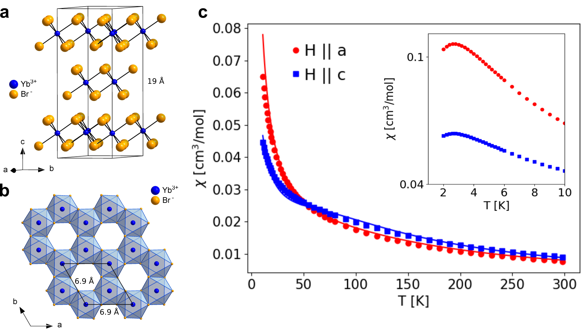
Figure 1: Fig.1 $|$ Magnetic susceptibility, crystal electric field and crystal structure. a, View along [210] on the unit cell of YbBr₃. b, Yb³⁺ honeycomb layer. c, Temperature dependence of the magnetic susceptibility $\chi$ of YbBr₃ for field orientations along the a- and c-axes. Solid lines are the calculated single-ion susceptibilities based on the crystal field (CEF)-parameters (Suppl.Info.). Inset: Measured low-temperature susceptibility showing a rounded peak around $T=2.75\;{\rm K}$.

Figure 2

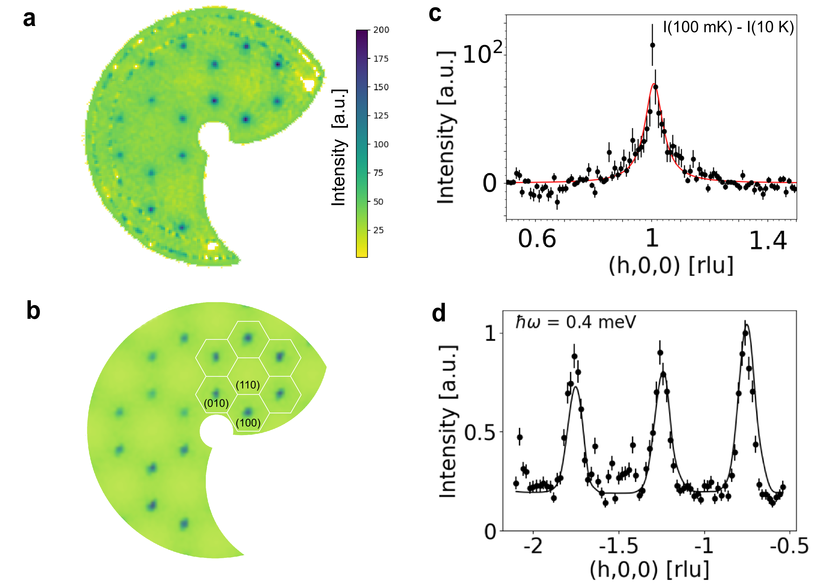
Figure 2: Fig.2 $|$ Magnetic diffuse scattering and correlation length. a, Magnetic diffuse scattering in YbBr₃ in the [h,k,0] plane at T = 100 mK, after subtraction of the nuclear Bragg contribution. b, Calculated magnetic diffuse scattering based on the spin-wave model including exchange and dipolar interactions. c, Cut through the diffuse scattering along the (h,0,0) direction. The line is a fit to the data with a Lorentzian function. [Note that the presence of paramagnetic scattering at 10 K leads to a negative background in the 100 mK data after subtraction]. d, Constant-energy scan for $\rm\hbar\omega=0.4\leavevmode\nobreak\ meV$ in YbBr₃ at T = 250 mK showing well-defined low energy excitations. The solid line represents the computed inelastic neutron scattering cross-section. Observed small peaks are due to spurious scattering and are not included in the model calculation.

Figure 3

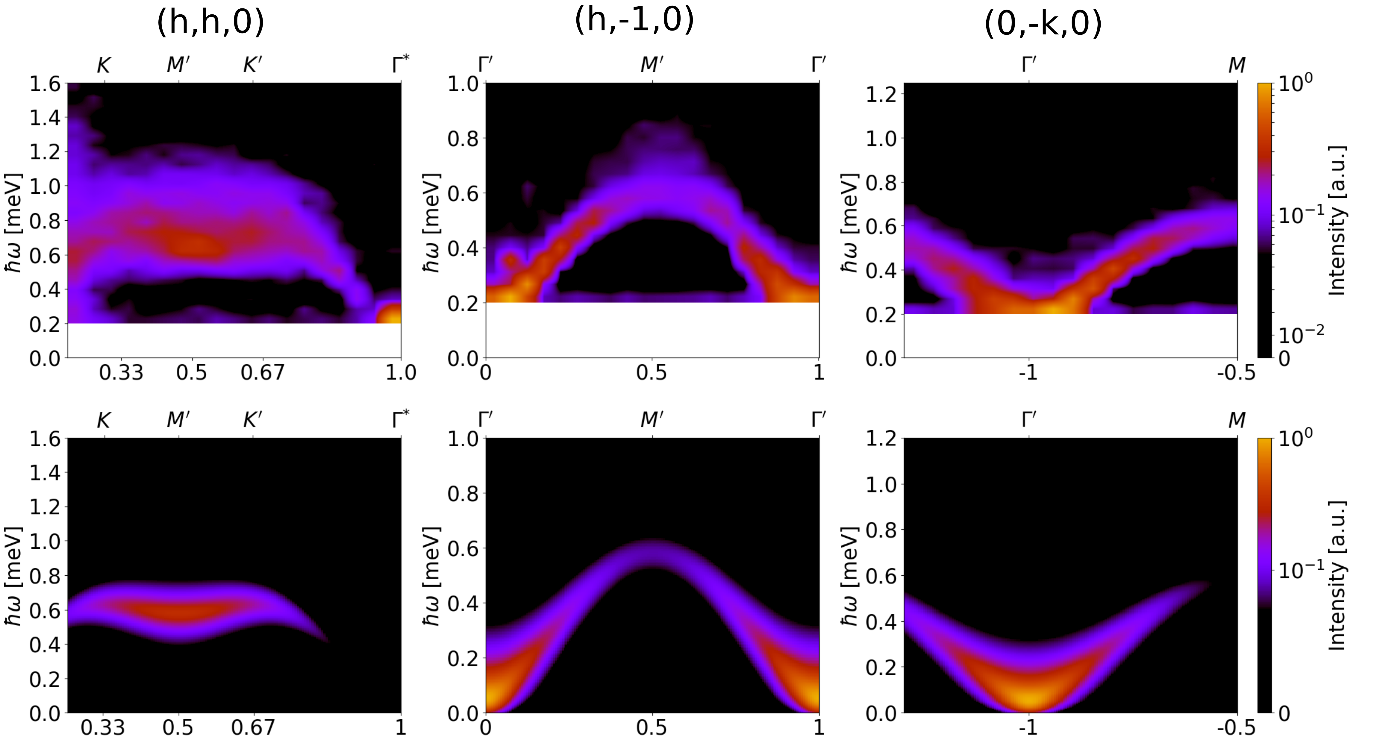
Figure 3: Fig.3 $|$ Magnetic excitations along high symmetry directions. False color plot of the observed (top) and calculated (bottom) inelastic neutron cross section of the magnetic excitations in YbBr₃ at $T=0.25$ K. The intensity is shown on a logarithmic scale. Note the existence of a continuum of excitations around $(1/2,1/2,0)$ and $(1/2,-1,0)$ which is not described by spin waves and is indicative of plaquette fluctuations (cf. Fig. 5).

Figure 4

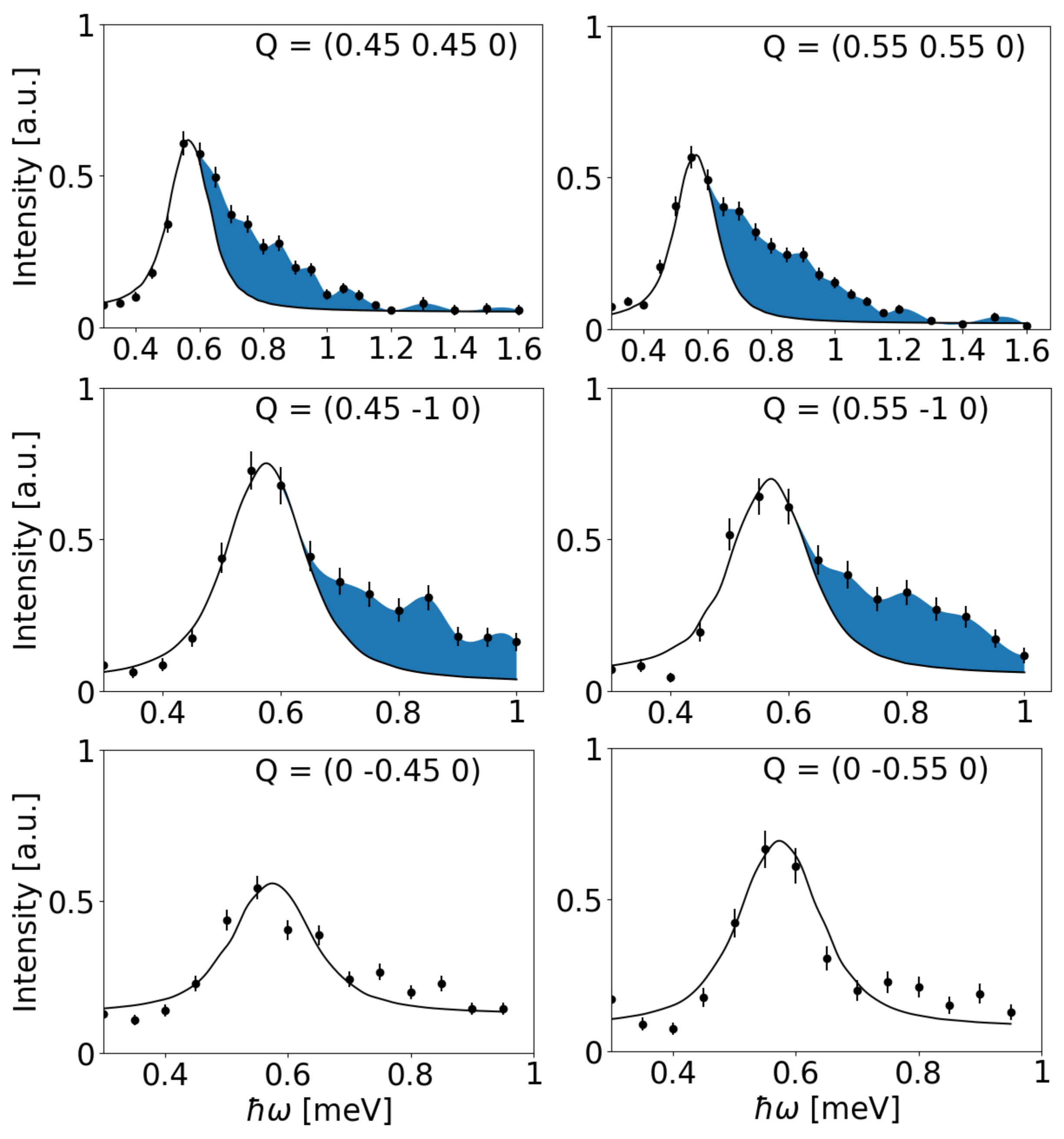
Figure 4: Fig.4 $|$ Excitation continuum near the Brillouin zone boundary. Observed and simulated magnon spectra based on the spin-wave model explained in the text. The lines are fits to the data with a Lorentzian function. An intrinsic line-width of $0.1\leavevmode\nobreak\ {\rm meV}$ was used for the simulation. The shaded area indicates the continuum of excitations.

Figure 5

Figure 5: Fig.5 $|$ Calculated neutron form factor for a plaquette. The neutron form factor of an Yb₆ hexagon calculated within the random-phase approximation and assuming Néel order on the plaquette. The directions of the neutron measurement are indicated by white arrows: cut I corresponds to $(h,h,0)$, cut II is $(0,-k,0)$ and cut III is $(h,-1,0)$. High-symmetry points are labeled similar to Fig. 3. Basis vectors of the reciprocal lattice are denoted as ${\bf a^{*}},{\bf b^{*}}.$

Supplementary materials

The supplementary materials include

• Section S1: Crystal structure

• Section S2: Magnetic susceptibility

• Section S3: Crystal electric field

• Section S4: Magnetic ground-state

• Section S5: Magnetic excitations

• Table 1: Structural parameters of YbBr₃ determined on HRPT at room temperature

• Fig. S1: Crystal electric field and magnetic susceptibility fit for YbBr₃

• Fig. S2: Dependence of the energy gap as a function of easy-plane anisotropy

• Fig. S3: Calculated susceptibility for a Yb₆ hexamer

• References

Section S1: Crystal structure

YbBr₃ crystallizes with the BiI₃ layer structure in the rhombohedral space group $R\bar{3}$ (148) with lattices parameters of $a$ = 6.97179(18)$\rm\leavevmode\nobreak\ \AA$ and $c$ = 19.1037(7)$\rm\leavevmode\nobreak\ \AA$ at room temperature. The lattice parameters are in good agreement with powder [1] and crystal [2] diffraction data found in literature. The unit cell contains six Yb³⁺ ions on site (6c) at (0, 0, z), (0, 0, z) + (2/3, 1/3, 1/3) and (0, 0, z) + (1/3, 2/3, 2/3) with z = 0.1670(2). The Yb ions have C₃ point symmetry and form two-dimensional (2D) honeycomb lattices perpendicular to the $c$-axis, see Fig. 1. Yb³⁺ has a distorted octahedral coordination by Br^- ions which are located on site (18f) at (x, y, z) with x=0.3331(5), y=0.3131(5), and z=0.08336(15). Surprisingly, the distance between Yb³⁺-Br^- varies by less than $10^{-2}\,{\rm\AA}$, however the Br^--Yb³⁺-Br^- bond angles differ significantly between 87.3^∘ and 91.1^∘. The crystallographic parameters determined on HRPT are are summarized in Table 1.

Section S2: Magnetic Susceptibility

The temperature dependence of the static susceptibility $\chi$ is shown in Fig. 1c for magnetic field orientations in-plane ($a$-axis) and out-of-plane ($c$-axis). $\chi T$ values (not shown) increase with temperature and do not saturate up to 300 K. The values at 300 K are 2.282 and 2.687 cm³K/mol along the a- and c-axes, respectively. The average of 2.417 cm³K/mol is slightly below the expectation value of 2.572 cm³K/mol for the ${}^{2}F_{7/2}$ ground-state of Yb³⁺. At lower temperature a maximum in the $\chi$ versus $T$ curves is observed at $T=2.75\leavevmode\nobreak\ {\rm K}$, see the inset in Fig. 1c. We have calculated the temperature dependence of the static susceptibility for an Yb₆ honeycomb with the exchange parameters determined from the spin-wave analysis and easy-plane anisotropy parameters g_a/g_c = 1.25. We find that the susceptibility has a broad maximum around T $\simeq$ 4 K and reproduces the experimental $\chi$ (T) above 5 K well, as shown in Fig. S2.

Section S3: Crystal electric field (CEF)

The electrostatic potential originating from the ions surrounding the Yb³⁺ ion can be modelled with Stevens operators

$$\begin{aligned} H_{CEF}=\sum_{l,m}B_{l}^{m}O_{l}^{m}\end{aligned}$$

with $B_{l}^{m}=\gamma_{l}^{m}\theta_{l}$ and $\theta_{l}$ the Stevens coefficients. For the $C_{3}$ point group symmetry of the Yb site only the parameters [8] $B_{2}^{0},B_{4}^{0},B_{4}^{\pm 3},B_{6}^{0},B_{6}^{\pm 3},B_{6}^{\pm 6}$ are non-zero. From the inelastic neutron scattering measurement we determined 3 CEF excitations at $E_{1}=14.5$ meV, $E_{2}=25$ meV and $E_{3}=29$ meV. We first used the susceptibility $\chi(T)$ for the determination of the CEF Hamiltonian. From a least-square fit to $\chi_{a}$ and $\chi_{c}$ where $a$ and $c$ denote the crystallographic axis we obtain $\gamma_{2}^{0}$ = -5.14 meV, $\gamma_{4}^{0}$ = -0.59 meV, $\gamma_{4}^{+3}$ = 57.43 meV, $\gamma_{4}^{-3}$ = 51.31 meV, $\gamma_{6}^{0}$ = 6.09 meV, $\gamma_{6}^{+3}$ = 50.21 meV, $\gamma_{6}^{-3}$ = 55.56 meV, $\gamma_{6}^{+6}$ = 33.9 meV, $\gamma_{6}^{-6}$ = 42.4 meV. In agreement with the Kramers theorem the CEF splits the $J=7/2$ multiplet of the Yb³⁺ ion into 4 doublets. The calculated CEF-levels are at $15.16$ meV, $24.75$ meV, and $28.88$ meV, respectively. From a subsequent fit of the inelastic neutron data we obtain very similar values, $\gamma_{2}^{0}$ =-6.49 meV, $\gamma_{4}^{0}$ = -0.51 meV, $\gamma_{4}^{+3}$ =58.53 meV, $\gamma_{4}^{-3}$ =52.12 meV, $\gamma_{6}^{0}$ = 6.01 meV, $\gamma_{6}^{+3}$ = 48.11 meV, $\gamma_{6}^{-3}$ = 56.30 meV, $\gamma_{6}^{+6}$ = 33.21 meV, $\gamma_{6}^{-6}$ = 41.12 meV. We show in Fig. S1 a comparison between calculated and observed neutron scattering intensities. We point out that first excitated CEF-level has a double-peak structure in YbBr₃ that is not explained by our model. It is conceivable that this peak structure is caused by a phonon, and as it also resembles the CEF levels[9] of YbCl₃ this issue requires further investigation. Nevertheless the CEF-model presented here provides an adequate description of the temperature dependence of the static susceptibility. In addition we performed a point charge calculation based on the program multiX [3]. In agreement with the susceptibility measurements, calculations show that at high temperatures anisotropy is small in YbBr₃ with easy-plane anisotropy developing below T = 50 K. At T = 4 K, we obtain $\chi_{a}\approx 1.3\chi_{c}$.

Section S4: Magnetic ground-state

In mean field theory, the classical ground-state is given by the eigenvectors of the largest eigenvalue $\lambda$ (q) of the Fourier transform of the interaction matrix $\overline{\overline{M}}$(q) [4, 5, 6]. Based on the Hamiltonian $H_{\rm h}+H_{\rm dip}$, $\lambda$ (q) has a maximum at Q₀ = (0,0,0) which agrees with the diffuse scattering observed in YbBr₃ (cf. Fig. 2a). We find that the dipolar energy becomes independent of the distance between the Yb-planes for a lattice parameter $c>20\leavevmode\nobreak\ {\rm\AA}$, which shows that the 2D limit is reached in YbBr₃ and inter-layer interactions can be neglected.

Section S5: Magnetic excitations

Because of the large separation between the ground-state and the first CEF doublet, the magnetic properties of YbBr₃ can be approximated by a spin $S=1/2$. Choosing a local coordinate frame with the $\zeta$-axis oriented along a given spin direction, the non-zero elements of the single-ion susceptibility matrix are $\chi_{0}^{\xi\xi}(\omega)=\chi_{0}^{\eta\eta}(\omega)$ and $\chi_{0}^{\xi\eta}(\omega)=-\chi_{0}^{\eta\xi}(\omega)$ which correspond to excitations transverse to the (local) spin direction. Within mean-field approximation,

$$\chi^{\xi\xi}_{0}(\omega) = {1\over 2}\frac{\Delta}{\Delta^{2}-(\omega+i\epsilon)^{2}}$$ (8)

$$\chi_{0}^{\xi\eta}(\omega) = {i\over 2}\frac{\omega+i\epsilon}{\Delta^{2}-(\omega+i\epsilon)^{2}},$$ (9)

with $\Delta\equiv\Delta_{i}=-\langle S_{\zeta}\rangle\sum_{j}{\cal J}_{\zeta\zeta}(i,j)$ the local field acting on a given Yb moment with ${\cal J}$ defined in Eq. (1) and $\epsilon$ the finite line width of the excitations.

Within linear spin-wave theory, the dipole-dipole interactions induce a gap in the spin-wave dispersion [34, 7]. With a Yb magnetic moment of $\rm 2\leavevmode\nobreak\ \mu_{B}$, the dipolar interactions produce a spin gap at the zone center $\rm\sim 200\leavevmode\nobreak\ \mu eV$. The easy-plane anisotropy favors alignment of the spins in the hexagonal plane. The spin gap opened by $H_{\rm dip}$ is reduced by the easy-plane anisotropy. At $g_{\rm crit}\sim 0.985$ the spin gap is minimal and below that value the spins rotate into the basal plane, see Fig. S2. The easy-plane anisotropy lifts the degeneracy of the spin wave branches at the zone center and the splitting increases with increasing anisotropy.

Supp. Tables

Table 1: Structural parameters of YbBr₃ determined on HRPT at room temperature

Name	x	y	z	occ.
Yb1	0	0	0.33289(21)	0.317(3)
Yb2	0	0	0	0.009(0)
Br	0.35362(57)	0.00022(60)	0.08325(15)	1

Supp. Figures

S1: Crystal electric field.

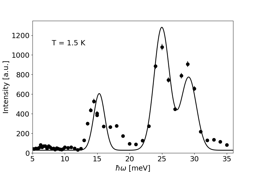
Figure 6: Fig. S1 $|$ Yb³⁺ crystal electric field in YbBr₃. Crystal electric field (CEF) excitations measured by inelastic neutron scattering. The solid line is the calculated intensity for the CEF-parameters given in Suppl. Info. S3.

S2: Dependence of the energy gap as a function of easy-plane anisotropy.

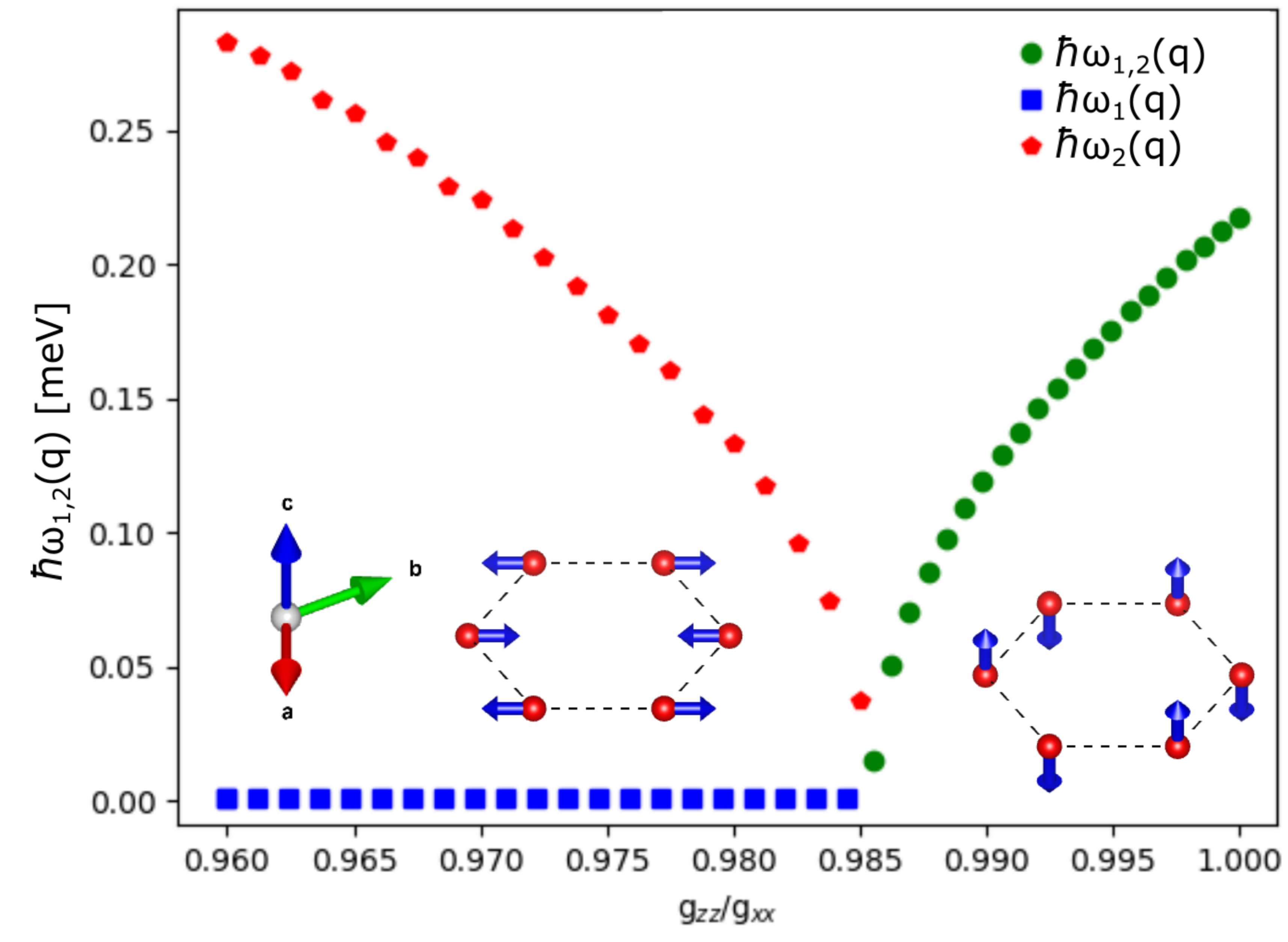
Figure 7: Fig. S2 $|$ Dependence of the energy gap as a function of easy-plane anisotropy. Above $\rm g_{zz}/g_{xx}$ = 0.985 = $\rm g_{crit}$, the calculated branches $\rm\omega_{1}(q)$ and $\rm\omega_{2}(q)$ are degenerate while for $\rm g_{zz}/g_{xx}<g_{crit}$ the two spin-wave branches split. All points are calculated with a precision of $\sim$ 0.005 meV. The magnetic configurations shown in the figure correspond to a Néel antiferromagnet with spins aligned along the c-axis for $\rm g_{zz}/g_{xx}>$ 0.985 and in the hexagonal plane for $\rm g_{zz}/g_{xx}<$ 0.985.

S3: Calculated susceptibility for a Yb₆ hexamer.

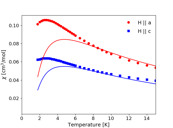
Figure 8: Fig. S3 $|$ Calculated susceptibility for a Yb₆ hexamer. The measured low-temperature magnetic susceptibility is shown together with the calculation (solid lines) for a single plaquette with $S=1/2$, and the Hamiltonian $H_{\rm h}+H_{\rm dip}$ of the main text.

References

References

- 1. Dowling, J.P. & Milburn, G.J. Quantum technology: the second quantum revolution. Phil. Trans. R. Soc. Lond. A 361, 1655-1674 (2003).
- 2. Kitaev, A.Y. Fault-tolerant quantum computation by anyons. Ann. Phys. 303, 2-30 (2003).
- 3. Nayak, C., Simon, S.H., Stern, A., Freedman, M., & Das Sarma, S. Non-Abelian anyons and topological quantum computation. Rev. Mod. Phys. 80, 1083 - 1159 (2008).
- 4. Kitaev, A.Y. Anyons in an exactly solved model and beyond. Ann. Phys. 321, 2-111 (2006).
- 5. Savary, L. & Balents, L. Quantum spin liquids: a review. Rep. Prog. Phys. 80, 016502-016568 (2016).
- 6. Tsyrulin, N. et al. Quantum Effects in a Weakly Frustrated S = 1/2 Two-Dimensional Heisenberg Antiferromagnet in an Applied Magnetic Field. Phys. Rev. Lett. 102, 197201 (2009).
- 7. Anderson, P.W. Resonating valence bonds: A new kind of insulator? Mat. Res. Bull. 8, 153-160 (1973).
- 8. Anderson, P.W. et al. The physics behind high-temperature superconducting cuprates: the ‘plain vanilla’ version of RVB. J. Phys.: Condens. Matter 16, R755–R769 (2004).
- 9. Senthil, T.,Vishwanath, A., Balents, L., Sachdev, S. & Fisher, M. P. A. Deconfined Quantum Critical Points. Science 303, 1490 (2004).
- 10. Mulder, A., Ganesh, R., Capriotti, L. & Paramekanti, A. Spiral order by disorder and lattice nematic order in a frustrated Heisenberg antiferromagnet on the honeycomb lattice. Phys. Rev. B 81, 214419 (2010).
- 11. Fouet, J.B., Sindzingre, P. & Lhuillier, C. An investigation of the quantum model on the honeycomb lattice. Eur. Phys. J. B 20, 241-254 (2001).
- 12. Merino, J. & Ralko, A. Role of quantum fluctuations on spin liquids and ordered phases in the Heisenberg model on the honeycomb lattice. Phys. Rev. B 97, 205112 (2018).
- 13. Wang, F. Schwinger boson mean field theories of spin liquid states on a honeycomb lattice: Projective symmetry group analysis and critical field theory. Phys. Rev. B. 82, 024419 (2010).
- 14. Albuquerque, A.F. et al. Phase diagram of a frustrated quantum antiferromagnet on the honeycomb lattice: Magnetic order versus valence-bond crystal formation. Phys. Rev. B 84, 024406 (2011).
- 15. Ganesh, R., van den Brink, J. & Nishimoto, S. Deconfined Criticality in the Frustrated Heisenberg Hamiltonian Honeycomb Antiferromagnet. Phys. Rev. Lett. 110, 127203 (2013).
- 16. Ferrari, F. & Becca, F. Dynamical properties of Néel and valence-bond phases in the model on the honeycomb lattice. arXiv:1912.09310 (2019).
- 17. Tennant, D.A., Perring, T.G., Cowley, R.A. & Nagler, S.E. Unbound Spinons in the S = 1/2 Antiferromagnetic Chain KCuF3. Phys. Rev. Lett. 70, 4003-4006 (1993).
- 18. Dender, D.C., Hammar, P.R., Reich, D.H., Broholm, C. & Aeppli, G. Direct Observation of Field-Induced Incommensurate Fluctuations in a One-Dimensional S = 1/2 Antiferromagnet. Phys. Rev. Lett. 79, 1750-1753 (1997).
- 19. Mendels, P.& Bert, F. Quantum kagome frustrated antiferromagnets: One route to quantum spin liquids. C. R. Physique 17, 455-470 (2016).
- 20. Shimizu, Y., Miyagawa, K., Kanoda, K., Maesato, M. & Saito, G. Spin Liquid State in an Organic Mott Insulator with a Triangular Lattice. Phys. Rev. Lett. 91, 107001 (2003).
- 21. Villain, J. Insulating Spin Glasses. Z. Physik B 33, 31-42 (1979).
- 22. B. Canals & C. Lacroix, Pyrochlore Antiferromagnet: A Three-Dimensional Spin Liquid. Phys. Rev. Lett. 80, 2933-2936 (1998).
- 23. Banerjee, A. et al. Proximate Kitaev quantum spin liquid behaviour in a honeycomb magnet. Nature Materials 15, 733-741 (2016).
- 24. Singh, Y. et al. Relevance of the Heisenberg-Kitaev Model for the Honeycomb Lattice Iridates A3IrO3. Phys. Rev. Lett. 108, 127203 (2012).
- 25. Kitagawa, K. et al. A spin–orbital-entangled quantum liquid on a honeycomb lattice. Nature 554, 341-345 (2018).
- 26. Ganesh R., Nishimoto S., & van den Brink J. Plaquette resonating valence bond state in a frustrated honeycomb antiferromagnet, Phys. Rev. B 87, 054413 (2013).
- 27. Collins, M.R. Magnetic Critical Scattering (Oxford University Press, 1989).
- 28. Mattsson, A., Fröjdh, P. & Einarsson, T. Frustrated honeycomb Heisenberg antiferromagnet: A Schwinger-boson approach. Phys. Rev. B 49, 3997-4002 (1994).
- 29. Ghorbani, E., Shahbazi, F. & Mosadeq, H. Quantum phase diagram of distorted J1-J2 Heisenberg S = 1/2 antiferromagnet in honeycomb lattice: a modified spin wave study. J. Phys.: Cond. Mat. 28, 406001 (2016).
- 30. Mourigal, M. et al. Fractional spinon excitations in the quantum Heisenberg antiferromagnetic chain. Nat. Phys. 9, 435-441 (2013).
- 31. Han, T.-H. et al. Fractionalized excitations in the spin-liquid state of a kagome-lattice antiferromagnet. Nature 492, 406-410 (2012).
- 32. Weber, T., Georgii, R. & Böni, P. Takin: An open-source software for experiment planning, visualization, and data analysis. SoftwareX5, 121-126 (2016).
- 33. Ferrari, F., Bieri, S. & Becca, F. Competition between spin liquids and valence-bond order in the frustrated spin-1/2 Heisenberg model on the honeycomb lattice. Phys. Rev. B 96, 104401 (2017).
- 34. Pich, C. & Schwabl, F. Order of two-dimensional isotropic dipolar antiferromagnets. Phys. Rev. B 47, 7957-7960 (1993).
- 35. Zhitomirsky, M.E. & Chernyshev, A.L. Colloquium: Spontaneous magnon decays. Rev. Mod. Phys. 85, 219-243 (2013).
- 36. Lee, S.-H. et al. Emergent excitations in a geometrically frustrated magnet. Nature 418, 856-858 (2002).
- 37. Ferrari, F. & Becca, F. Spectral signatures of fractionalization in the frustrated Heisenberg model on the square lattice. Phys. Rev. B. 98, 100405 (2018).
- 38. Senthil, T., Balents, L., Sachdev, S., Vishwanath, A. & Fisher, M.P.A. Quantum criticality beyond the Landau-Ginzburg-Wilson paradigm. Phys. Rev. B. 70, 144407 (2004).
- 39. Bishop, R.F., Li, P.H.Y. & Campbell, C.E. Valence-bond crystalline order in the model on the honeycomb lattice. J. Phys.: Condens. Matter 25, 306002 (2013).
- 40. Krämer, K.W. et al. Noncollinear two- and three-dimensional magnetic ordering on the honeycomb lattices of (). Phys. Rev. B 60, R3724-R3727 (1999).
- 41. Meyer, G. Advances in the Synthesis and Reactivity of Solids, 2, 1-26 (Elsevier science & technology, Oxford, 1994).
- 42. Jensen, J. & Macintosh, A.R. Rare Earth Magnetism (Clarendon Press, Oxford, 1991).
Acknowledgments
Funding: The financial support by the Swiss National Science Foundation under grant no. SNF 200020172659 is gratefully acknowledged. Author contributions: D.C., L.K., M.K., B.R. and C.W. performed the neutron experiments. Crystal growth and characterization was done by K.W.K.. Theoretical calculations were performed by B.D., B.R., C.W., O.W., and H.B.B.. Data analysis and discussion of the results was done by all authors. All authors contributed to the writing of the manuscript. Competing interests: The authors declare no competing interests. Data and materials availability: All data needed to evaluate the conclusions in the paper are present in the paper and/or the Supplementary Materials. Additional data related to this paper may be requested from the authors.

References

- 1. Meyer, G. Private communication to powder diffraction data base (PDF2), no. [42-0968] (1990).
- 2. Brenner, M. Kinetische Studien zu Phasenumwandlungen zwischen polymorphen Formen von YbBr2 sowie die Bestimmung der Kristallstruktur von YbBr3. Dissertation Universität Karlsruhe (1997).
- 3. Uldry, A., Vernay, F. & Delley, B. Systematic computation of crystal-field multiplets for x-ray core spectroscopies. Phys. Rev. B 85, 125133 (2012).
- 4. Reimers, J.N. Diffuse-magnetic-scattering calculations for frustrated antiferromagnets. Phys. Rev. B 46, 193-202 (1992).
- 5. Kadowaki, H., Ishii, Y., Matsuhira, K. & Hinatsu, Y. Neutron scattering study of dipolar spin ice Ho2Sn2O7: Frustrated pyrochlore magnet. Phys. Rev. B 65, 144421 (2002).
- 6. Enjalran, M. & Gingras, M.J.P. Theory of paramagnetic scattering in highly frustrated magnets with long-range dipole-dipole interactions: The case of the Tb2Ti2O7 pyrochlore antiferromagnet. Phys. Rev. B 70, 174426 (2004).
- 7. Pich, C. & Schwabl, F. Spin-wave dynamics of two-dimensional isotropic dipolar Honeycomb antiferromagnets. JMMM 148, 30-31 (1995).
- 8. E. Bauer & M. Rotter, “Magnetism of Complex Metallic Alloys: Crystalline Electric Field effects”, in: Book Series on Complex Metallic Alloys Vol. 2, ed. E. Belin-Ferr, World Scientific (2009).
- 9. Sala, G. et al., Crystal field splitting, local anisotropy, and low-energy excitations in the quantum magnet YbCl3, Phys. Rev. B 100, 180406 (2019).