Also at ]e.rapisarda@iaea.org
The measurement of the quadrupole moment of 185Re and 187Re from the hyperfine structure of muonic X rays
Abstract
The hyperfine splitting of the transitions in muonic 185,187Re has been measured using high resolution HPGe
detectors and compared to state-of-the-art atomic theoretical predictions. The spectroscopic quadrupole moment has been extracted using
modern fitting procedures and compared to the values available in literature obtained from muonic X rays of natural rhenium.
The extracted values of the nuclear spectroscopic quadrupole moment are 2.07(5) barn and 1.94(5) barn, respectively for
185Re and 187Re.
This work is part of a larger effort at the Paul Scherrer Institut towards the measurement of the nuclear charge radii
of radioactive elements.
pacs:
32.30.Rj, 32.10.Fn, 36.10.Ee, 21.10.KyI Introduction
It is well known that muonic X rays can be used as a sensitive means to determine the charge radius of a nucleus. Moreover if the hyperfine structure (hfs) can be resolved, then the distribution of the magnetic dipole (MD) and electric quadrupole (EQ) moments in the nucleus can be investigated as well. All stable elements and few unstable elements have been studied by muonic X-ray spectroscopy. Rhenium is the last stable element whose nuclear charge radius has not been measured with muonic X rays Angeli and Marinova (2013). Since Re is a strongly-deformed nucleus, the muonic X-ray spectrum is complicated by the so-called dynamic hyperfine splitting Jacobsohn (1954); Wilets (1954). This effect is particularly sizeable in muonic atoms and is due to the fact that the quadrupole interaction between muon and nucleus has non-vanishing off-diagonal elements which link the ground state and low-lying excited states of the nucleus. The effect leads to a mixing of the nuclear states due to the similar energy scale between the atomic binding energies and the nuclear excitation energies resulting in a dynamic hyperfine splitting even for nuclei which have zero spin in the ground state where no hfs is to be expected. As a result of the dynamic hyperfine splitting, the extraction of the nuclear charge parameters from the transition in deformed nuclei requires a more elaborated analysis compared to spherical nuclei as shown in Acker (1966); McKee (1969); Tanaka et al. (1984a) and references therein.
The only existing measurement of muonic X rays of rhenium was performed on a natural rhenium target and aimed at the
extraction of the spectroscopic quadrupole moment from the analysis of the hyperfine splitting of the
transitions Konijn et al. (1981).
The full muonic X-ray spectrum of isotopically pure targets of 185Re and 187Re has been recently measured by the
muX collaboration at the Paul Scherrer Institut (PSI) for the first time, with the aim to extract the main properties
of the nuclear charge distribution from muonic spectroscopy, which are still missing in literature.
In this paper we present the analysis of the hyperfine splitting of the muonic transitions yielding
the spectroscopic quadrupole moment of 185,187Re.
The analysis of the and muonic transitions and the extraction of the nuclear charge radius
will be reported elsewhere.
The muonic X-ray spectra of the two isotopically pure rhenium targets,
a major improvement over the analysis presented in Ref. Konijn et al. (1981), analysed with state-of-the-art theoretical predictions and
fitting procedures have shown that the
fit of the hfs of the transitions, and consequently the extracted value of the quadrupole moment,
is very sensitive to the inclusion of weaker muonic transitions not included in the analysis of Ref. Konijn et al. (1981).
Particular care has also been taken on the determination of the peak shape of the germanium detectors
from muonic X-ray data, while in Konijn et al. (1981) off-line calibration runs with sources were used.
The measurements reported in this article are part of a larger effort going on at PSI (muX project) to perform
muonic atom spectroscopy on radioactive elements (usually available only in microgram quantities) aiming,
as first test cases, at the precise measurement of the nuclear charge radius of 226Ra and 248Cm Adamczak et al. (2018); Skawran et al. (2019).
Section II reviews the theory of the muonic atoms in order to establish the notation used in the hfs formalism and also includes a discussion of the various corrections to the energy levels beyond the predictions of the Dirac equation. Section III.1 describes the apparatus used in obtaining the X-ray spectra, Section III.2 describes the data-reduction methods and also includes the 208Pb muonic X-ray results which where used as a calibration standard for the 185,187Re spectra. Section IV details the fit of the transitions of the 185,187Re spectra using the hfs formalism of Section II.2 and the extraction of the nuclear quadrupole moments.
II Theory
II.1 Fine structure
In order to predict the transition energies and probabilities as well as their dependence on the nuclear quadrupole moment theoretically, the bound muon is described as a Dirac particle. As the mass of the muon is about 207 times larger than the electron’s mass , the energy scale for muonic atoms is a factor 207 larger than regular electronic atoms. The Bohr radius of the muon is smaller than the one of the electron by the same factor, which leads to a significant enhancement of nuclear effects.
The bound muon is described by the Dirac equation
| (1) |
where are the Dirac matrices, is the electrostatic potential caused by the nuclear charge distribution, and and are muonic energies and wavefunctions, correspondingly. Here stands for the principal quantum number, while the relativistic angular quantum number is introduced as a bijective function of the orbital angular momentum and the total muon angular momentum as , and is the component of . For a spherically symmetric potential, the radial components and the angular part can be separated, and therefore the solution can be written as Greiner (2000)
| (2) |
The angular part of the wave function is described by spherical spinors , and the radial wave functions are normalised with an integral
| (3) |
For a Coulomb potential , Eq. (1) can be solved analytically and gives the well-known formula for the Dirac-Coulomb energies
| (4) |
where is the fine-structure constant and the nuclear charge. However, predictions of the muonic spectra have to include the finite size of the nucleus already in the Dirac equation. The deformed Fermi distribution
| (5) |
has proven to be very successful in the description of the level structure of heavy muonic atoms, see e.g. Hitlin et al. (1970); Tanaka et al. (1984a, b), and is also used in this work. Here, is the skin thickness parameter, the half-density radius, the deformation parameter, a normalisation constant and the spherical harmonics. The corresponding spherically symmetric part of the nuclear potential is
| (6) |
It has been shown, that , with , is a good approximation for most of the nuclei Beier (2000). Then, and are chosen such that the root-mean-square radius of the distribution agrees with the literature value Angeli and Marinova (2013) and the quadrupole moment agrees with a given value, which is obtained by fitting to the experimental data as described in Section II.5. The connection between the charge distribution of Eq. (5) and the spectroscopic quadrupole moment is
| (7) |
where is the nuclear angular momentum number and are the Legendre polynomials.
With the potential of Eq. (6), Eq. (1) can be solved only numerically. For this purpose the dual-kinetic-balance method Shabaev et al. (2004) has been used in this work. For the muon in the state the binding energy including finite-size effect is almost 50% smaller than the value assuming a point Coulomb potential. For the states the reduction is on a level of 0.1%, and even smaller for the states.
The order- quantum electrodynamics contributions are the self-energy (SE) and the vacuum polarisation (VP) corrections. For atomic electrons they are usually of the same order of magnitude. For muons, however, the VP correction is much larger as the virtual electron-positron pair production is less suppressed due to their low mass compared to the muon’s mass Borie and Rinker (1982). The dominant VP contribution (first order in and ) is called Uehling correction, and can be described by the potential Elizarov et al. (2005)
| (8) |
This potential can be directly included into the Dirac equation of Eq. (1) by adding it to , therefore directly accounting all iterations Indelicato (2013) of the Uehling potential into the muonic binding energies. In the same way, the higher-order contributions to the VP correction, namely the Wichmann-Kroll (order ) potential Wichmann and Kroll (1956); Fullerton and Rinker (1976) in the point-like approximation and the Källen-Sabry (order ) potential Källen (1955) for a spherically symmetric nuclear charge distribution were included in the Dirac equation, using the expressions from Indelicato (2013). Since both the Wichmann-Kroll and the Källen-Sabry corrections to the energy levels of muonic atoms are small, the neglected nuclear model dependence was estimated to be insignificant.
The recoil correction, i.e., the effect of finite nuclear mass and the resulting motion of the nucleus, was accounted following the approach used in Refs. Friar and Negele (1973); Borie and Rinker (1982); Michel et al. (2017).
The effect of the surrounding electrons on the binding energies of the muon, commonly referred to as electron screening, was estimated following Ref. Vogel (1973); Michel et al. (2017) by calculating an effective screening potential from the charge distribution of the electrons and using this potential in the Dirac equation for the muon. The atomic electrons primarily behave like a charged shell around the muon and the nucleus; thus every muon level is mainly shifted by a constant term, which is not observable in the muonic transitions. The main contribution to the screening potential comes from the electrons, since their wave functions have the largest overlap with the muonic wavefunctions.
The results of our calculations for rhenium for the total binding energies and for the individual contributions are presented in Table 1.
| 1013.125 | -1.175 | 3.547 | -0.067 | 0.026 | -0.062 | |
| 1000.021 | -0.478 | 3.374 | -0.065 | 0.024 | -0.064 | |
| 1000.021 | -0.004 | 2.930 | -0.064 | 0.021 | -0.048 | |
| 993.697 | -0.001 | 2.859 | -0.063 | 0.020 | -0.049 | |
| 640.055 | -0.003 | 1.459 | -0.035 | 0.010 | -0.123 | |
| 636.806 | -0.001 | 1.425 | -0.034 | 0.010 | -0.125 | |
| 636.806 | -0.000 | 1.215 | -0.033 | 0.009 | -0.098 | |
| 634.883 | -0.000 | 1.199 | -0.033 | 0.009 | -0.099 |
II.2 Hyperfine structure
The hyperfine splitting appears as a result of the interaction of the bound muon with the magnetic dipole (MD) and electric quadrupole (EQ) moments of the nucleus. In contrast to the electronic atom, where the MD splitting dominates over the EQ splitting (see e.g. Korzinin et al. (2005)), the muonic MD splitting is suppressed because the magnetic moment of the muon is times smaller than the electronic one.
As the hyperfine splitting mixes the nuclear and muonic quantum numbers, they are not conserved anymore and cannot be used for a proper description of the energy levels. Therefore, a combined mixed state with total angular momentum and its projection is introduced as
| (9) |
where are the Clebsch-Gordan coefficients.
The diagonal matrix elements of the EQ hyperfine operator Korzinin et al. (2005); Michel et al. (2017); Michel and Oreshkina (2019) are determined by the formula:
| (10) | ||||
| (13) | ||||
Here, is the quadrupole distribution function, which describes the deviations from a point-like quadrupole and depends on a deformed charge distribution as
| (14) |
where and . Similarly, the MD hyperfine splitting can be calculated by the formula Korzinin et al. (2005); Michel et al. (2017); Michel and Oreshkina (2019)
| (15) | ||||
| (16) | ||||
with the proton mass , nuclear magneton , nuclear magnetic dipole moment , and its distribution function . For the simple model of a homogeneous distribution of the dipole moment inside the nucleus, reads
| (17) |
where for RN the nuclear charge radius is commonly used. In practice, both the electric and magnetic distribution functions were calculated for several nuclear models to estimate the model uncertainty using the values of the nuclear magnetic moment for 185Re and for 187Re Stone (2016).
II.3 Dynamical splitting
For the states in heavy muonic atoms, the EQ hyperfine splitting, the fine-structure splitting, and the low-lying nuclear rotational band can be on the same energy scale of few hundreds of keV. This leads to a strong mixing of the muonic and nuclear levels caused by the EQ hyperfine interaction, commonly called dynamic hyperfine splitting Hitlin et al. (1970).
For the analysis of the transitions from to in this work, the hyperfine splitting is much smaller than the nuclear transitions between low-lying nuclear states, hence the excited nuclear states do not need to be considered. However, there is still a residual mixing of the muonic states of Eq. (9) due to higher-order hyperfine interaction. This can be included by rediagonalisation of the EQ and MD interaction in the considered initial and final states.
For the set of all considered initial/final states, the non-diagonal EQ and MD matrix elements of the and operators have been calculated Michel and Oreshkina (2019); Michel (2018). Then, the rediagonalisation has been performed separately for each value of , since the MD and EQ interaction are diagonal in . After the rediagonalisation, the unperturbed states are mixed and can be described as
| (18) |
where is the number of initial/final states, and the coefficients diagonalise the hyperfine interaction. The quantum numbers and , describing the total angular momentum of the nucleus-muon system, are still well-defined. In this work, the EQ matrix elements were also corrected with the order VP contribution using the approach of Michel and Oreshkina (2019).
II.4 Transition probabilities and line intensities
The muonic transition rates due to spontaneous emission of a photon between states with defined total angular momentum F from an initial state to a final state , summed over the projections and (to simplify the formalism from now on), are Johnson (2007)
| (19) | ||||
Here, is the energy difference between the initial and final state, is the total angular momentum of the photon and Johnson (2007) is the multipole transition operator. corresponds to an electric transition, whereas stands for a magnetic transition.
In the experimental spectra, the number of counts measured in the peak is proportional to the transition intensities, which are the product of the transition probability and the population of the initial states. The transition probability per unit time can be calculated ab initio with Eq. (19). In this work, the relative population of the muonic fine structure states within a state was assumed statistical, i.e. proportional to , whereas the relative population of the and states was left as free parameter and determined by fitting the experimental spectra (see Section IV.2).
II.5 Dependence of observables on quadrupole moment
After a muon is captured in a highly excited state and starts cascading towards its ground state, there is an intermediate region, () where finite nuclear size effects are still rather small while the muon is not significantly influenced by the surrounding atomic electrons. This intermediate region (in our case ) is well suited for the extraction of quadrupole moments Dey et al. (1979); Konijn et al. (1979).
Four fine-structure states together with the nuclear ground state with define the initial states. The energies were calculated as described in Section II.1, II.2, and II.3; including finite size effects, VP (Uehling, Källen-Sabry, Wichmann-Kroll in point-like approximation, quadrupole electronic-loop Uehling), SE, electron screening, and recoil effect; with the rediagonalisation of the EQ and MD hyperfine interaction. The same procedure was repeated for the final states with , i.e. and . The transition probabilities were calculated from each initial to each final state with Eq. (19) for E1 (, ) and M1 (, ) transitions, assuming a statistical initial population in and . With this approach, the entire spectrum of interest can be calculated for a given spectroscopic quadrupole moment .
For the comparison of the theoretical predictions with the measured experimental spectra, the full calculations for each transition were performed for several values of the quadrupole moment in the proximity of the expected value and a quadratic function is fitted for every transition energy and intensity as
In this way, the fitting coefficients, in addition to the first-order EQ splitting, contain also the information about MD splitting and higher-order EQ interaction, whereas in Ref. Konijn et al. (1981) only the term linear in the quadrupole moment was considered. The resulting dependencies for the transition energies and for the relative intensities are given in Table 3, in Table 4, respectively for 185Re and 187Re, and in Table 5.
III Experimental setup and analysis
III.1 Setup
The experiment was performed at the HIPA facility of the Paul Scherrer Institut
and is part of the ongoing muonic X-ray study of radioactive elements.
The negative muon beam was obtained from the decay of pions produced in the collisions of
590 MeV protons on a thick graphite target. The momentum-analysed muon beam
was transported to the E1 area and consisted mostly of muons and electrons. The electron
contamination, which can be a source of background, was efficiently
removed using a Wien filter separator placed at around 15 m before the target.
As a result, a high purity negative muon beam could be obtained.
The energy of the muon beam was tuned to a momentum of around 29 MeV/c in order to maximise
the stopping in the targets.
The typical intensity at the detection setup at the given momentum was in the order of 104 per second.
The beam exits the beam line through a 75 m thick mylar window and travels in air for around 10 cm
before being stopped in the target.
The incoming negative muons and electrons were identified before impinging on the target
by the muon counting detector, a 500 m thick plastic scintillator
with a 66 cm2 active area read out by photomultipliers and placed in air in close
vicinity to the end of the beam line. Given the small thickness, the signals induced by the muons
could be easily separated with a threshold cut from the much smaller signals induced by the electrons.
The muon counting detector was used as start detector for the coincidence measurements (see Section IV).
In addition, at the same position, a second scintillator, 2 mm thick with a 99 cm2 active area and
a central hole of 45 mm, so that the muon beam was passing through this hole before being stopped in the target, was used
as veto detector to produce anti-coincidence conditions on the muonic X-ray spectra.
Measurements were done with three isotopically pure targets of 185Re (97.6%), 187Re (99.4%) and
208Pb (99.6%). The 208Pb target was used for the energy calibration and served as a means of
checking drifts and possible malfunctions.
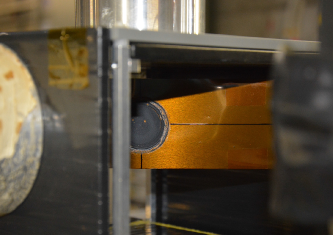
The isotopes were purchased in the form of a powder (500 mg)
in the case of rhenium and in the form of an irregularly shaped ingot (1g) in the case of lead.
The rhenium powder was first finely ground in a mortar and then mixed with 60 to 70 mg of epoxy on a Kapton foil.
The mixture was subsequently covered with a Teflon foil and, loaded with some weights, slowly brought into
a disk-like shape of around 30 mm diameter. The lead piece was cold-pressed and hammered into a disk of 40 mm diameter.
The targets were then glued onto a Kapton foil and mounted on a PVC frame which was inserted in a target holder
at 45∘ with respect to the direction of the beam.
A picture of one of the rhenium targets mounted on the target holder can be seen in Fig. 1.
Typical muon stopping rates were 2500/s for the 208Pb target and 900/s for the rhenium targets.
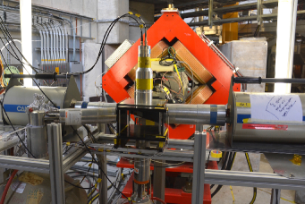
The muonic X rays following the muonic cascade were detected by two single crystal
high-purity germanium (HPGe) coaxial detectors
with relative efficiency of 20% and 75% placed in close vicinity to the
target at 90∘ (GeR) and -90∘ (GeL), respectively,
with respect to the direction of the incoming beam. Fig. 2 shows the detector arrangement. Two more
HPGe detectors and a LaBr3 scintillator were also operated but they are not used for the analysis
presented here. The typical energy resolution for 1.3 MeV
radiation was 2.1 keV and 2.9 keV (FWHM), for the 20% and 75% detector, respectively.
The absolute photo-peak efficiency for the
359.8 keV line, the most intense transition in the hfs
observed in 185Re, was 0.2% and 0.5% for GeR and GeL, respectively,
for the given geometry. The efficiency
calibration was performed using standard sources of 137Cs, 60Co, 88Y and 152Eu.
Typical single rates in the germanium detectors were 500 and 1000 counts per second, respectively.
Finally four plastic scintillator counters 5 mm thick and 18 18 cm2 large were placed around
the target in a box-like structure. The signals from these plastic scintillator counters were used in anti-coincidence with
the germanium detectors signals and allowed removal of background events in the X-ray spectra mainly produced
by the electrons emitted in the muon decay.
The readout system was based on the STRUCK SIS3316 digitiser and the MIDAS data acquisition system MID . This is a VME module providing 16 spectroscopic channels with a 250 MHz 14 bits sampling ADC each. The signals from each of the detector preamplifiers are passed directly to the SIS3316 modules. The smaller signals from GeL were routed through a fast amplifier in order to match better the dynamic range of the digitiser. The filtering is performed digitally using algorithms implemented on field programmable gate arrays (FPGA) on the SIS3316 board, a fast filter being used for triggering, timing and pile-up rejection and a slow filter for energy determination. With a data acquisition running in trigger-less mode, time and energy were recorded for all detector signals above a certain threshold. Additionally, for the germaniums and LaBr3 scintillator, the traces were also read out. Prompt and delayed muonic X-ray spectra of the germanium detectors were built by imposing conditions in the time difference between the germanium detector and the muon counter. In a similar way the anti-coincidence conditions of the germanium signals with the signal of the other scintillator counters were built and applied to reduce background in the X-ray energy spectra.
III.2 Calibration
The usual experimental sequence involved collecting data from a rhenium target for 4 hours (4 runs),
with two hours calibration runs with the lead target directly preceding and following each group of 4 runs with rhenium.
The main purpose of these calibration runs was to verify that there
had been no substantial gain shift during the target runs which might cause loss of energy resolution.
Line shifts due to electronic instability were checked using a 60Co radioactive source and the 2614.5 keV ray
in the natural radioactive background. The source was placed near the target and its -rays appeared in the muonic X-ray
spectrum. In order to sum all individual calibration runs, each run must be corrected for any relative gain shift and shift
of the base line. This was done by first locating the centroids of the 1332.5 and 2614.5 keV rays
appearing in all runs.
By comparing the centroids of the peaks from these runs with a preselected run, one can determine the gain shift and the shift of
the zero offset. To ensure sufficient statistics the spectra were evaluated every two runs.
After correcting gain shifts, the spectra of the different runs were summed. Typical gain shifts were in the order of 0.03%.
In the energy calibration the well-established energies of the muonic X rays in
208Pb, 16O and 12C were used.
Muonic X rays from oxygen and carbon were observed in the prompt energy spectra due to the accidental hit of the muon beam
on materials surrounding the targets.
IV Results
By applying time conditions in the coincidence events between the Ge detectors and the entrance muon counter,
it was possible to select prompt Ge events such as muonic X rays, where the muon stop and the subsequent atomic X rays
are instantaneous within the time resolution of the detectors, and nuclear rays resulting from the muon-capture
process which exhibits a characteristic lifetime of about 80 ns at Z75 Suzuki and Measday (1987).
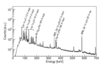
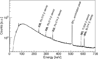
Fig. 3 shows a portion of the -ray spectrum in the energy region of interest
measured in the Ge detector positioned at 90∘ (GeR) with the 185Re (top) and 208Pb (bottom)
targets in prompt coincidence (400 ns) with the entrance muon counter. In addition Ge detector events not in coincidence with
the entrance muon counter within 2 s were selected to produce room background -ray spectra,
as shown in Fig. 4. In Fig. 3 the transitions belonging to muonic 208Pb and 185Re are indicated
together with the muonic X rays of 35Cl, 27Al, 16O, 14N and 12C. The assignment of lines
was based on previously known transitions Kessler et al. (1975); Backenstoss et al. (1967).
Other strong lines in Fig. 3 and Fig. 4 come from the decay of nuclei produced in the muon capture reaction or
from room background. One of the strongest lines in the spectrum is the
511 keV ray, originating mainly from the annihilation of the positrons produced in the
electromagnetic cascade of the high-energy electron emitted in the muon decay.
Data for around 60 hours were collected with muons on the 208Pb target, 38 hours on the 185Re target
and 59 hours on the 187Re target.

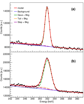
IV.1 Line shape
Since the hyperfine splitting is the result of the convolution of many transitions, particular care has to be taken in describing
the experimental line shape of each transition.
The mathematical form of the line shape should represent the response of the Ge detector plus a background term.
In this respect, the model used consists of a Gaussian peak , a step-like shelf ,
and a Hypermet function Maxwell (1997); Salathe and Kihm (2016). The latter is added to account
for a possible tail, which decays exponentially below the peak’s centroid and is produced by incomplete charge collection
and ballistic deficits. The model function was fitted to the shape of the peak by
using RooFit Verkerke and Kirkby (2003). RooFit implements its data models in terms of probability density functions (PDFs),
which are by definition unit normalised. The model function describing the number of counts in the peak at energy
may be written as
| (20) | ||||
where
In these formulae is the mean of the Gaussian, the Gaussian width and the slope of the exponential
tail. denotes the fraction of the line shape having the Gaussian form and = (1- )
the fraction having the exponential tail. The parameter A denotes the amplitude of the step which
is proportional to the number of events in the signal. The parameter B is introduced to describe a constant background.
This description was valid for most of the transitions except for the few cases where a linear function provided a better
description.
The variables , , , the number of events in the signal , ,
and the two amplitudes A and B are free parameters of the model.
Since the response of the germanium detector is energy dependent, a consistent set of parameters
(, , , A)
describing the experimental line shape was obtained by fitting four nuclear transition lines which lie close in energy to the
muonic transitions of interest. These are the 265.8 keV transition from muon capture in 208Pb observed in the prompt
spectrum with the 208Pb target and the 351.9 keV, 583.2 keV and 609.3 keV transitions observed in the room background.
The natural line width of these lines is assumed to be negligible compared to the experimental resolution.
The four transitions were fitted simultaneously with the Gaussian width expressed as a linear function of the
peak position Knoll (2010).
The set of line-shape parameters obtained with this procedure are reported in Table 2.
Fig. 5 shows the 351.9 keV transition observed in the spectrum of the GeR and
the GeL detectors together with the fit function described in Eq. (20).
Similar fits were obtained for the 265.8, 583.2 and 609.3 keV transitions.
It is important to note that by determining the line shape from the set of data collected
with beam on target, we ensure the appropriate representation of the detector response in the presence of beam.
In previous analyses Konijn et al. (1981); Dixit (1971) the line shape used to determine the position of the muonic
X rays was the same as the one used for the calibration source lines collected in dedicated runs.
With this procedure one relies on the strong assumption that the
detector response stayed unchanged between the X-ray runs and the calibration runs.
| Fit parameter | GeL | GeR |
|---|---|---|
| 0.00024(1) | 0.00034(1) | |
| (keV) | 0.918(7) | 0.466(4) |
| (keV) | 2.2(2) | 5.0(8) |
| 0.893(6) | 0.93(1) | |
| A (1/keV) | 0.0137(7) | 0.010(1) |
The muonic X-ray peaks are broader than the calibration source lines or background lines due to the natural width
of the muonic energy states. Since the intrinsic X-ray line shape is Lorentzian, the muonic X rays were fitted using
the experimental line shape of Eq. (20) where the Gaussian component is modified into a
Gaussian-convoluted Lorentzian (resulting in a Voigt profile) with calculated transition widths.
The typical natural line widths are 80 eV for the ,
and transitions and 150 eV for the
and transitions.
IV.2 The hyperfine splitting in 185,187Re
The analysis of the hyperfine splitting was performed in higher muonic levels n=5 and n=4.
The and hfs
complexes appear as two bumps located at around 360 keV (see Fig. 3) and they have been analysed together.
The and the levels of 185,187Re are sixfold split as in this case and
l = 5, 4. Taking the selection rules into account for transitions within both hf complexes, the resulting
X-ray pattern consists of thirty members.
In the analysis of the hfs spectrum the correction for
the presence of the weaker , and
multiplets has to be taken into account, as they coincide in energy.
The hfs spectra analysed consisted therefore of 76 lines originating from five multiplets which
were fitted using for each line the empirical line shape described by Eq.(20)
corrected for the radiative width. The background constant was common for all the lines.
The intensity and energy position of the individual members of the hf multiplets relative to the
most intense transition for each multiplet were calculated using the
formalism described in Section II.2 and in Section II.5. The values are given in Table 3
and in Table 4 for 185Re and 187Re, respectively.
The multiplets were then correlated in energy to the transition
in using the values given in Table 5.
It should be noted that the energy splittings of the hyperfine transitions in the
multiplet are around a factor three larger than the values given in Ref. Konijn et al. (1981) whereas the calculations for the
other multiplets agree. The difference can be due to a mistake in reporting the values.
The intensity of the three multiplets originating from the state has been correlated to the intensity
of the most intense hyperfine transition in
assuming the hypothesis that the states within a l multiplet are statistically populated; similarly
the intensity of two multiplets originating from the has been correlated to the intensity
of the most intense hyperfine transition in .
The relative intensity of the lines within a l multiplet does not depend on the initial distribution of the cascade and
therefore they were kept fixed in the fitting procedure. On the other hand, no assumption can be made on the
relative population of the and states as it depends on the details of the
atomic cascade of muons which are still rather uncertain, particularly as to the exact beginning of the cascade.
Following this procedure, the description of the hfs could be reduced to five parameters which are
the energy of the hyperfine transition in ,
the quadrupole moment, the two intensities of the and
transitions and the number of background events.
They were used as free parameters and varied until the best fit to the spectra was found.
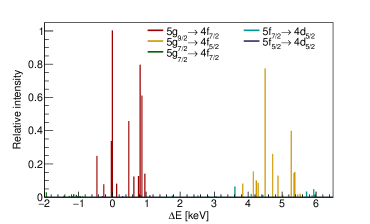
Fig. 6 shows the theoretical prediction of the hfs of the five multiplets considered in
the present analysis calculated for = 2.21 barn. In the figure the intensity ratio
over is set equal to 0.06 as obtained from a cascade calculation Akylas and Vogel (1978)
with initial statistical distribution at N = 20 and width of the K-shell refilling process of 25 eV. Different initial
conditions of the cascade calculations give a range of values between 0.06 and 0.08.
| FFi | ||||||||||
|---|---|---|---|---|---|---|---|---|---|---|
| FFi | ||||||||||
|---|---|---|---|---|---|---|---|---|---|---|
| I = 0.333 | I = 0.257 | I = 0.0095 | I = 0.020 | I = 0.001 |
| 185Re | ||||
| 360.214 | 364.663 | 358.280 | 364.417 | 361.141 |
| -0.174 | -0.160 | -0.178 | -0.440 | -0.448 |
| 0.0 | 0.004 | -0.000 | -0.002 | -0.004 |
| 187Re | ||||
| 360.215 | 364.663 | 358.280 | 364.412 | 361.136 |
| -0.175 | -0.160 | -0.178 | -0.439 | -0.448 |
| 0.0 | 0.004 | -0.000 | -0.002 | -0.004 |
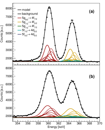
The measured spectrum of 185Re together with the result of the fit is shown
in Fig. 7 for the two Ge detectors used. The fit for 187Re is shown in Fig. 8.
Tables 6 and 7 summarise the values of the fit parameters.
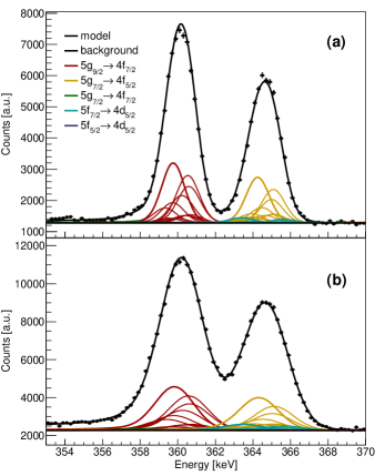
The isotopic impurity of the targets was included in the fitting procedure by having
the hfs spectrum described by a double complex (one for each isotope) with one multiplet slightly shifted with
respect to the other. The value of the shift is proportional to the ratio of the quadrupole moments
of the two isotopes which was taken from literature. In the case of the 187Re, the fit parameters
were not affected by the inclusion of the small impurity of 185Re and it was therefore neglected in the final fit.
In addition to the five parameters mentioned above to describe the structure of the hfs, the step A of the line shape
was also left as free parameter. This because it was not possible to reproduce the hfs with the value extracted
from the line shape analysis. This effect might be due to the very different background between
the delayed spectrum (where the line shape analysis has been performed) and that of the prompt spectrum.
Reasonably good fits were obtained with per degree of freedom of 2.5 and 1.5 for GeR and GeL
in 185Re and 1.8 and 1.1 in 187Re.
The energy of the hyperfine transition
in multiplet obtained from the fit is 359.9(1) keV for GeL and
359.8(1) keV for GeR. These values are the same for the two rhenium isotopes and show that,
with the procedure described in Section III.2,
a very good energy calibration with precision at the level of 100 eV can be achieved.
The intensities of the transition relative to the
obtained from the fits are higher compared to the value of 6%
obtained from the calculation of the muonic cascade.
Such discrepancies are not surprising given the approximation of the cascade calculations
and were observed in similar analyses Dey (1975); Dey et al. (1979).
Moreover, possible resonance effects between nuclear and muonic states could modify significantly
the muonic cascade leading to anomalous intensity ratios. Such resonance effects are more likely to
occur in very deformed nuclei due to the dense nuclear excitation spectrum.
On the other hand, in the same isotope, the relative intensities deduced from the two detectors
differs up to 50%.
This inconsistency in the fitted relative intensities
has been taken into account by adding a systematic error to the
extracted quadrupole moment (see Section IV.3).
| Fit | GeR | GeL | ||||||||
|---|---|---|---|---|---|---|---|---|---|---|
| (barn) | RI | E7→6 (keV) | A (1/keV) | (barn) | RI | E7→6 (keV) | A (1/keV) | |||
| Full 111Full fit as described in Section IV.2. | 2.11(2) | 0.090(8) | 359.8(1) | 10-9 | 2.39 | 2.04(5) | 0.139(7) | 359.9(1) | 0.0051(4) | 1.51 |
| no | 2.11(2) | 0.090(8) | 359.8(1) | 10-9 | 2.34 | 2.06(4) | 0.137(7) | 359.9(1) | 0.0051(4) | 1.50 |
| no | 2.18(3) | 0.074(9) | 359.7(1) | 0.0009(6) | 3.85 | 2.17(4) | 0.122(7) | 359.8(1) | 0.0057(4) | 2.28 |
| no weak transitions 222The and multiplets are removed from the fit. | 2.18(3) | 0.076(9) | 359.7(1) | 0.0011(5) | 3.80 | 2.19(4) | 0.121(7) | 359.8(1) | 0.0058(4) | 2.22 |
| fix population333Relative intensity fixed to 0.14 for GeR and 0.09 for GeL. | 2.03(2) | 0.139 | 359.8(1) | 0.0014(4) | 2.85 | 2.12(4) | 0.090 | 359.8(1) | 0.0037(3) | 2.06 |
| Fit | GeR | GeL | ||||||||
|---|---|---|---|---|---|---|---|---|---|---|
| (b) | RI | E7→6 (keV) | A (1/keV) | (b) | RI | E7→6 (keV) | A (1/keV) | |||
| Full 111Full fit as described in Section IV.2. | 1.97(2) | 0.118(7) | 359.8(1) | 10-11 | 1.72 | 1.93(5) | 0.17(1) | 359.9(1) | 0.0043(6) | 1.25 |
| no | 1.98(2) | 0.118(7) | 359.8(1) | 10-10 | 1.62 | 1.96(4) | 0.168(9) | 359.9(1) | 0.0044(5) | 1.22 |
| no | 2.04(3) | 0.099(8) | 359.7(1) | 0.006(5) | 3.07 | 2.05(5) | 0.155(14) | 359.8(1) | 0.0050(6) | 1.92 |
| no weak transitions 222The and multiplets are removed from the fit. | 2.05(2) | 0.097(7) | 359.7(1) | 0.0001(3) | 2.99 | 2.07(5) | 0.154(9) | 359.8(1) | 0.0051(6) | 1.86 |
| fix population333Relative intensity fixed to 0.17 for GeR and 0.12 for GeL. | 1.90(2) | 0.170 | 359.8(1) | 0.0013(5) | 2.22 | 1.99(8) | 0.118 | 359.9(1) | 0.0026(5) | 1.62 |
IV.3 Quadrupole moments and uncertainty
The values of quadrupole moments with their statistical errors are collected in the
Tables 6 and 7.
To evaluate possible systematic errors of different parameters, like the line shape, the of the experimental line shape,
and the description of the background, their influence on the extracted value of the quadrupole moments was studied separately
in a systematic way and is reported in Table 8 for the two targets.
The effects were checked for small variations of the
with respect to the values reported in the Tables 6 and 7.
The effect of variation in the modeling of the background and the line shape turned out to be negligible
with respect to the value of the quadrupole moment.
The sensitivity of our results to the assumed background
was examined by comparing the hfs parameters obtained with our constant background model with those using a linear
or quadratic form of the background.
The influence of the experimental line shape was investigated by sampling the parameters describing the
line shapes. Out of 1000 sampled line shapes, around 300 could simultaneously fit the shape of the background lines
with reasonable values of .
Each of these line shapes was then used in the fit of the hf complex and the distribution of the extracted
values of the quadrupole moments was fitted with a Gaussian.
The centroid of the quadrupole moment distribution showed no variation with respect to the quadrupole
moment given by the best line shape and the sigma of the Gaussian distribution was taken as uncertainty.
In a similar way, the effect of the was checked by sampling the values within its statistical
uncertainty while leaving fixed the other parameters of the line shape. Also in this case the centroid of the distribution of the
extracted quadrupole moments showed no variation with respect to the value of the best line shape
but with a larger uncertainty.
Finally, most sensitive was the relative intensity of the versus
transition. As described in Section IV.2 the fits of the two detectors do not converge to
the same ratio. In Table 8 the variation of the quadrupole moment obtained when the ratio
versus is fixed to the medium value of the two detectors
is reported. This variation has been added in the systematic uncertainty.
| Effect | GeR | GeL | ||
|---|---|---|---|---|
| (b) | error (b) | (b) | error (b) | |
| Bkg model | 0.0 | 0.01 | 0.0 | 0.01/ 0.03 |
| Line shape | 0.0 | 0.01 | 0.0 | 0.01/ 0.02 |
| 0.0 | 0.02/ 0.03 | 0.0 | 0.07/ 0.06 | |
| RI | -0.04/ -0.03 | 0.04/ 0.03 | 0.03/ 0.03 | 0.03/ 0.03 |
| Total | -0.04/ -0.03 | 0.05 | 0.03/ 0.03 | 0.08 |
The final quadrupole moments with their uncertainty are
= 2.07 0.02 (stat) 0.05 (syst)
= 1.94 0.02 (stat) 0.05 (syst)
and
= 2.07 0.05 (stat) 0.08 (syst)
= 1.96 0.05 (stat) 0.08 (syst)
for GeR and GeL, respectively. Given the larger uncertainty in GeL, a combined analysis of the
two detectors is clearly not worthwhile.
The ratio of the quadrupole moments was not fixed in our fits and amounts to 2.07(5)/1.94(5) = 1.067(35)
in very good agreement with the very precise value of 1.056709(17) reported by S.L. Segel Segel (1978).
The extracted -values are smaller compared to the values of = 2.21(4) barn and
= 2.09(4) barn reported in Ref. Konijn et al. (1981).
Two weak multiplets namely and have
been introduced in the present analysis which were not included in the previous work.
Their effect on the extracted quadrupole moment is reported in Table 6 and Table 7.
While the inclusion of the very weak does not modify the results of the quadrupole moment,
the multiplet has stronger influence and it leads to a lower value of quadrupole moment
explaining the discrepancy to the values reported in Konijn et al. (1981).
The addition of the multiplet in the fitting of the hfs was necessary in order to
properly reproduce the rising slope at low energy of the experimental spectrum as can be inferred by the
significantly higher value of reduced obtained when this
transition is removed from the fit. This effect clearly shows that the isotopically pure muonic X-ray spectra
could be sensitive to transitions of relative intensity of only a few %. Since the fitted hfs spectrum is not reported
in Konijn et al. (1981) neither are the values of , we cannot judge the quality of the fit
and consequently the sensitivity of that experimental spectrum to weaker transitions.
V Conclusions
The hfs of the X-ray transition in muonic 185,187Re has been investigated.
The extracted values of the quadrupole moments have been determined based on high-quality isotopically
pure muonic X-ray spectra of 185,187Re and state-of-the-art theoretical calculations and fitting procedures.
The quadrupole moments = 2.07(5) barn and = 1.94(5) barn are measured for 185,187Re, respectively.
The disagreement with values in literature extracted with the same procedure has been understood
from the higher sensitivity of the muonic X-ray spectra of isotopically pure targets to weak hyperfine transitions.
The measurement of the hyperfine splitting of muonic X rays allows the extraction of the quadrupole moment of the nucleus
to a rather high precision compared to the hyperfine splitting in electronic systems
because they do not suffer from the uncertainty in the calculation of a multi-electron system
for the determination of the electric field gradient at the nucleus and the polarisation
of the electron core. Nevertheless, we have pointed out that
particular care has to be taken in the estimation of the systematic errors
for what concerns the description of the detector response and the relative intensity of the muonic transitions.
This work is part of the muX project which currently pursues at PSI the possibility to extend muonic atom
spectroscopy to elements available in microgram quantities, with a special emphasis on 226Ra.
Acknowledgements.
We gratefully thank L. Simons for many valuable discussions. This work was supported by the Paul Scherrer Institut through the Career Return Programme, by the Swiss National Science Foundation through the Marie Heim-Vögtlin grant No. 164515 and the project grant No. 200021_165569, by the Cluster of Excellence ”Precision Physics, Fundamental Interactions, and Structure of Matter” (PRISMA EXC 1098 and PRISMA+ EXC 2118/1) funded by the German Research Foundation (DFG) within the German Excellence Strategy (Project ID 39083149). FW has been supported by the German Research Foundation (DFG) under Project WA 4157/1. Most of the theory results in this article are part of the PhD thesis work of NM, which was published at the Heidelberg University, Germany. The experiment was performed at the E1 beam line of PSI. We would like to thank the accelerator and support groups for the excellent conditions. Technical support by F. Barchetti, F. Burri, M. Meier and A. Stoykov from PSI and B. Zehr from the IPP workshop at ETH Zürich is gratefully acknowledged.References
- Angeli and Marinova (2013) I. Angeli and K. Marinova, Atomic Data and Nuclear Data Tables 99, 69 (2013).
- Jacobsohn (1954) B. Jacobsohn, Phys Rev 15, 1637 (1954).
- Wilets (1954) L. Wilets, Kgl. Danske Videnskab Selskab, Mat-Fys. Medd. 29, 1 (1954).
- Acker (1966) H. L. Acker, Nucl. Phys. 87, 153 (1966).
- McKee (1969) R. McKee, Phys. Rev. 180, 1139 (1969).
- Tanaka et al. (1984a) Y. Tanaka, R. M. Steffen, E. B. Shera, W. Reuter, M. V. Hoehn, and J. D. Zumbro, Phys. Rev. C 29, 1830 (1984a).
- Konijn et al. (1981) J. Konijn et al., Nucl. Phys. A 360, 187 (1981).
- Adamczak et al. (2018) A. Adamczak et al., EPJ Web Conf 193, 04014 (2018).
- Skawran et al. (2019) A. Skawran et al., Il Nuovo Cimento C 42, 125 (2019).
- Greiner (2000) W. Greiner, Relativistic Quantum Mechanics, 3rd ed. (Springer-Verlag, Berlin Heidelberg, 2000).
- Hitlin et al. (1970) D. Hitlin, S. Bernow, S. Devons, I. Duerdoth, J. W. Kast, E. R. Macagno, J. Rainwater, C. S. Wu, and R. C. Barrett, Phys. Rev. C 1, 1184 (1970).
- Tanaka et al. (1984b) Y. Tanaka, R. M. Steffen, E. B. Shera, W. Reuter, M. V. Hoehn, and J. D. Zumbro, Phys. Rev. C 29, 1897 (1984b).
- Beier (2000) T. Beier, Physics Reports 339, 79 (2000).
- Shabaev et al. (2004) V. M. Shabaev, I. I. Tupitsyn, V. A. Yerokhin, G. Plunien, and G. Soff, Phys. Rev. Lett. 93, 130405 (2004).
- Borie and Rinker (1982) E. Borie and G. A. Rinker, Rev. Mod. Phys. 54, 67 (1982).
- Elizarov et al. (2005) A. A. Elizarov, V. M. Shabaev, N. S. Oreshkina, and I. I. Tupitsyn, Nucl. Instrum. Methods Phys. Res. B 235, 65 (2005).
- Indelicato (2013) P. Indelicato, Phys. Rev. A 87, 022501 (2013).
- Wichmann and Kroll (1956) E. H. Wichmann and N. M. Kroll, Physical Review 101, 843 (1956).
- Fullerton and Rinker (1976) L. W. Fullerton and G. A. Rinker, Phys. Rev. A 13, 1283 (1976).
- Källen (1955) G. Källen, K. Dan. Vidensk. Selsk. Mat.-Fys. Medd. 29, No (1955).
- Friar and Negele (1973) J. Friar and J. Negele, Physics Letters B 46, 5 (1973).
- Michel et al. (2017) N. Michel, N. S. Oreshkina, and C. H. Keitel, Phys. Rev. A 96, 032510 (2017).
- Vogel (1973) P. Vogel, Phys. Rev. A 7, 63 (1973).
- Korzinin et al. (2005) E. Y. Korzinin, N. S. Oreshkina, and V. M. Shabaev, Physica Scripta 71, 464 (2005).
- Michel and Oreshkina (2019) N. Michel and N. S. Oreshkina, Phys. Rev. A 99 (2019).
- Stone (2016) N. J. Stone, Atomic Data and Nuclear Data Tables. 111-112, 1 (2016).
- Michel (2018) N. Michel, Nuclear structure and QED effects in heavy atomic systems, Ph.D. thesis, Ruprecht-Karls-Universität, Heidelberg (2018).
- Johnson (2007) W. R. Johnson, Atomic Structure Theory, 1st ed. (Springer, Berlin Heidelberg, 2007).
- Dey et al. (1979) W. Dey, P. Ebersold, H. Leisi, F. Scheck, H. Walter, and A. Zehnder, Nuclear Physics A 326, 418 (1979).
- Konijn et al. (1979) J. Konijn, J. Panman, J. Koch, W. V. Doesburg, G. Ewan, T. Johansson, G. Tibell, K. Fransson, and L. Tauscher, Nuclear Physics A 326, 401 (1979).
- (31) “Midaswiki,” https://midas.triumf.ca/MidasWiki/index.php/Main_Page, [Accessed: 21-November-2019].
- Suzuki and Measday (1987) T. Suzuki and D. F. Measday, Phys Rev C 35, 2212 (1987).
- Kessler et al. (1975) D. Kessler et al., Phys. Rev. C 11, 1719 (1975).
- Backenstoss et al. (1967) G. Backenstoss et al., Phys. Lett. 25B, 547 (1967).
- Maxwell (1997) J. L. C. J. A. Maxwell, Nucl. Instr. Meth. B 129, 297 (1997).
- Salathe and Kihm (2016) M. Salathe and T. Kihm, Nucl. Instr. Meth. A 808, 150 (2016).
- Verkerke and Kirkby (2003) W. Verkerke and D. P. Kirkby, “The roofit toolkit for data modeling,” arXiv:physics/0306116 (2003).
- Knoll (2010) G. F. Knoll, in Radiation detection and measurements (John Wiley & Sons, Inc., 2010) Section 12, pp. 426–429, forth ed.
- Dixit (1971) M. S. Dixit, An experimental test of the theory of muonic atoms, Ph.D. thesis, The University of Chicago, Chicago, Illinois (1971).
- Akylas and Vogel (1978) V. R. Akylas and P. Vogel, Comp. Phys. Comm. 15, 291 (1978).
- Dey (1975) W. Dey, Messung von Spektroskopischen Kerngrund-zustandsquadrupol-momenten mit Myonischen Atomen am Beispiel von 175Lu, Ph.D. thesis, Eidgenössischen Technischen Hochschule Zürich, Zürich (1975).
- Segel (1978) S. L. Segel, Phys Rev C 18, 2430 (1978).