Large and Ultra-compact Gauss-Bonnet Black Holes
with a Self-interacting Scalar Field

A. Bakopoulos${}^{\,(a)}$ , P. Kanti${}^{\,(a)}$  and N. Pappas${}^{\,(a,b)}$ 

^(a)Division of Theoretical Physics, Department of Physics,
University of Ioannina, Ioannina GR-45110, Greece

^(b)Nuclear and Particle Physics Section, Physics Department,
National and Kapodistrian University of Athens, Athens GR-15771, Greece

Abstract

We consider the Einstein-scalar-Gauss-Bonnet theory, and study the case where a negative cosmological constant is replaced by a more realistic, negative scalar-field potential. We study different forms of the coupling function between the scalar field and the Gauss-Bonnet term as well as of the scalar potential. In all cases, we obtain asymptotically-flat, regular black-hole solutions with a non-trivial scalar field which naturally dies out at large distances. For a quadratic negative potential, two distinct subgroups of solutions emerge: the first comprises light black holes with a large horizon radius, and the second includes massive, ultra-compact black holes. The most ultra-compact solutions, having approximately the 1/20 of the horizon radius of the Schwarzschild solution with the same mass, emerge for the exponential and linear coupling functions. For other polynomial forms of the scalar potential, the subgroup of ultra-compact solutions disappears, and the black holes obtained may have a horizon radius larger or smaller than the Schwarzschild solution depending on the particular value of their mass.

1 Introduction

In our quest for a fundamental theory of gravity, the generalised gravitational theories, containing extra fields or curvature terms compared to the traditional General Relativity (GR) [1, 2], provide a valuable framework of study. These theories are considered to be only effective theories of gravity which reduce to GR at the weak-field limit but predict modifications of it at regimes of strong curvature. The successful detection of gravitational waves during the recent years [3, 4] has provided an additional tool for the study and verification, or disproof, of these theories, and thus has refueled the interest in their predictions. In particular, since modifications are expected only at regimes of strong gravity, predictions for the existence of novel black-hole solutions or compact objects have attracted a wide interest in the community.

The study of generalised gravitational theories was initiated only a few years after the the classification of black-hole solutions in GR was completed, and included extensions of GR [5] and its connection to other fields [6]. Soon, solutions of black holes with additional characteristics, or “hair”, compared to those of GR were found [7, 8, 9]. The development of the superstring effective theory [10, 11, 12] gave an additional boost to the study of these theories, and led the way towards the discovery and study of a number of novel black-hole solutions [14, 15, 16, 17, 18, 13, 19, 20, 21, 22, 23, 24, 25] (see [26, 27, 28, 29] for a number of reviews). Most of these solutions were found in the context of generalised theories built around a scalar field with non-minimal couplings to gravity, and evaded the so-called “no scalar-hair” theorem [30]. Extending GR via the addition of a scalar field and gravitational terms has also been the core of the Horndeski [31] and Galileon [32] theories. In the context of these theories, the no-hair theorems were re-formulated [33, 34] but were again evaded, and additional black-hole solutions were constructed [35, 36, 37, 38].

The class of Einstein-scalar-Gauss-Bonnet (EsGB) theories, which include, apart from the Einstein term, a scalar field and the quadratic Gauss-Bonnet (GB) term, is a particularly simple but extremely rich family of generalised gravitational theories. It is characterised by the form of the coupling function between the scalar field and the GB term, which is not a priori fixed. Setting this coupling function to be of an exponential form leads to the dilatonic theory, in the context of which the dilatonic black holes [13], the first counter-example of the scalar no-hair theorem [30], were found. For a linear coupling function, the shift-symmetric Galileon black holes [37] were also derived. These solutions have the characteristic feature of scalar hair: a regular, non-trivial scalar field which is associated with the black hole, a feature forbidden by GR. The group of theories which may lead to such solutions was significantly expanded a few years ago, when it was demonstrated [39], both analytically and numerically, that the EsGB theories support black-hole solutions with a regular, non-trivial scalar hair for every form of the coupling function. In addition to this natural scalarisation of the solutions, spontaneous scalarisation of the corresponding GR solution was also shown to take place [40, 41].

A large number of additional works has appeared over the years, which studied novel black holes or compact objects in these, or similar, types of theories as well as their properties [42]-[141]. Apart from asymptotically-flat black-hole solutions, solutions with an asymptotic (Anti)-de Sitter behaviour have also been investigated [142]-[165]. In addition, the Einstein-scalar-Gauss-Bonnet theory has been shown to lead to a large number of families of wormhole solutions that require no exotic matter [166, 167]. Last, but not least, it supports compact, particle-like solutions with regular spacetimes, non-trivial scalar hair and a number of interesting observable features [159, 169, 170, 172, 173, 168, 171].

In a previous work [160], we studied the EsGB theory in the presence of a negative cosmological constant $\Lambda$, and demonstrated that black-hole solutions with an asymptotically Anti-de Sitter behaviour and a scalar hair arise as easily as their asymptotically-flat counterparts. In the present work, we will address the case where this constant energy density is replaced by a non-trivial potential for the scalar field. Our objective is to provide a more realistic scenario where the cosmological constant, usually introduced in an ad hoc way in the theory, is now replaced by a field potential. We will first pose the question of whether black holes, naturally scalarised, arise in the context of such a theory, and whether only specific forms of the scalar-field potential may support them. If novel black-hole solutions do emerge, we would like to investigate which features of the previously found solutions are still preserved and which are modified. To this end, we will consider a variety of polynomial forms for the scalar-field potential, and combine them with various forms of the coupling function between the scalar field and the GB term. Given that black-hole solutions arise in abundance in the case of a negative cosmological constant [160], here, we will consider only negative-definite forms of the scalar potential. Scalarised solutions in the presence of a positive scalar potential of quadratic and quartic form have been studied in [90] and [91], respectively. In the present context, it will also be of great interest to see whether the combined effect of the GB term with a scalar potential – of a form not physically preferred – will manage to support regular black-hole solutions.

Our analysis will demonstrate that this is indeed the case, and that in fact regular black holes with a scalar hair emerge for any combination of choices for the coupling function and form of negative scalar potential we have used. We will present families of robust solutions describing spacetimes with a regular horizon at one end and an asymptotically-flat limit at the other. The scalar field, its effective potential, the GB curvature-invariant term and all components of the energy-momentum tensor will be finite reducing to zero at large distances. The solutions obtained will be larger or smaller, compared to the Schwarzschild solution with the same mass, depending on the exact form of the scalar potential, the value of the black-hole mass and the branch they belong to. In the case of a negative, quadratic potential, and for all forms of coupling functions, we obtain solutions which belong to two subgroups: the first comprises light GB black holes with horizon radius and entropy larger than the ones of the corresponding GR solution, and the second includes the more massive black holes with an increasingly smaller horizon radius which terminates to a class of massive, ultra-compact black holes.

The outline of this work is as follows: in Section 2, we present our theoretical framework and in Section 3, we consider the form of the asymptotic solutions near the sought-for black-hole horizon and asymptotic infinity. In Section 4, we study their thermodynamical properties, and in Section 5, we present our numerical results for he black-hole solutions found and their properties. We finish with our conclusions and discussion of our results in Section 6.

2 The Theoretical Framework

In this work, we will study a general class of higher-curvature gravitational theories, which includes the Einstein-Hilbert term, given by the Ricci scalar curvature $R$, a scalar field $\phi$, and the quadratic Gauss-Bonnet term defined as

$$R^{2}_{GB}=R_{\mu\nu\rho\sigma}R^{\mu\nu\rho\sigma}-4R_{\mu\nu}R^{\mu\nu}+R^{2}\,,$$ (1)

in terms of the Riemann tensor $R_{\mu\nu\rho\sigma}$, the Ricci tensor $R_{\mu\nu}$ and the Ricci scalar $R$. Therefore, the action functional of the theory has the form

$$S=\frac{1}{16\pi}\int{d^{4}x\sqrt{-g}\left[R-\frac{1}{2}\,\partial_{\mu}\phi\partial^{\mu}\phi+f(\phi)R^{2}_{GB}-2\Lambda V(\phi)\right]}.$$ (2)

A general coupling function $f(\phi)$ provides a coupling of the scalar field to the GB term since the latter is a total derivative in four dimensions. We have also included in the theory a self-interacting potential $V(\phi)$ for the scalar field; this upgrades the usually assumed cosmological constant $\Lambda$ to a dynamical potential, with $\Lambda$ assuming now the role of a coupling constant. In the context of this work, we will consider only the case with $\Lambda<0$. Therefore, by setting $V(\phi)=1$, we recover the Einstein-scalar-GB theory in the presence of a negative cosmological constant [160].

The variation of the aforementioned action with respect to the metric tensor $g_{\mu\nu}$ and the scalar field $\phi$ leads to the gravitational field equations and the equation for the scalar field, respectively. These have the form:

$$G_{\mu\nu}=T_{\mu\nu}\,,$$ (3)

$$\nabla^{2}\phi+\dot{f}(\phi)R^{2}_{GB}-2\Lambda\dot{V}(\phi)=0\,.$$ (4)

In the above, $G_{\mu\nu}$ is the Einstein tensor and $T_{\mu\nu}$ is the energy-momentum tensor, given by the expression

$$T_{\mu\nu}=-\frac{1}{4}g_{\mu\nu}\partial_{\rho}\phi\partial^{\rho}\phi+\frac{1}{2}\partial_{\mu}\phi\partial_{\nu}\phi-\frac{1}{2}\left(g_{\rho\mu}g_{\lambda\nu}+g_{\lambda\mu}g_{\rho\nu}\right)\eta^{\kappa\lambda\alpha\beta}\tilde{R}^{\rho\gamma}_{\quad\alpha\beta}\nabla_{\gamma}\partial_{\kappa}f(\phi)-\Lambda V(\phi)\,g_{\mu\nu}\,.$$ (5)

We also note that the dot over the coupling function and potential denotes their derivatives with respect to the scalar field (i.e. $\dot{V}=dV/d\phi$). We have also used the definitions

$$\tilde{R}^{\rho\gamma}_{\quad\alpha\beta}=\eta^{\rho\gamma\sigma\tau}R_{\sigma\tau\alpha\beta}=\frac{\epsilon^{\rho\gamma\sigma\tau}}{\sqrt{-g}}\,R_{\sigma\tau\alpha\beta}\,,$$ (6)

and, for simplicity, we have employed units in which $G=c=1$.

We are interested in deriving regular, static, spherically-symmetric black-hole solutions with a non-trivial scalar field. The line-element of space-time will accordingly take the form

$${ds}^{2}=-e^{A(r)}{dt}^{2}+e^{B(r)}{dr}^{2}+r^{2}({d\theta}^{2}+\sin^{2}\theta\,{d\varphi}^{2})\,.$$ (7)

We will assume that the scalar field has the same symmetries as the metric tensor, and therefore $\phi=\phi(r)$. Both the coupling function $f(\phi)$ and the scalar potential $V(\phi)$ will be assumed at the moment to have a general form, and particular choices will be made in the forthcoming sections.

Employing the line-element (7), we may easily derive the non-vanishing components of the Einstein tensor; these are

$$G^{t}_{\;\,t} =\frac{e^{-B}}{r^{2}}(1-e^{B}-rB^{\prime}),$$ (8)

$$G^{r}_{\;\,r} =\frac{e^{-B}}{r^{2}}(1-e^{B}+rA^{\prime}),$$ (9)

$$G^{\theta}_{\;\,\theta} =G^{\phi}_{\;\,\phi}=\frac{e^{-B}}{4r}\left[r{A^{\prime}}^{2}-2B^{\prime}+A^{\prime}(2-rB^{\prime})+2rA^{\prime\prime}\right].$$ (10)

Throughout our analysis, the prime denotes differentiation with respect to the radial coordinate $r$. Next, using Eq. (5), we may find the components of the energy-momentum tensor $T^{\mu}_{\;\;\nu}$

$$T^{t}_{\;\,t}= -\frac{e^{-2B}}{4r^{2}}\left[\phi^{\prime 2}\left(r^{2}e^{B}+16\ddot{f}(e^{B}-1)\right)-8\dot{f}\left(B^{\prime}\phi^{\prime}(e^{B}-3)-2\phi^{\prime\prime}(e^{B}-1)\right)\right]-\Lambda V,$$ (11)

$$T^{r}_{\;\,r}= \frac{e^{-B}\phi^{\prime}}{4}\left[\phi^{\prime}-\frac{8e^{-B}\left(e^{B}-3\right)\dot{f}A^{\prime}}{r^{2}}\right]-\Lambda V,$$ (12)

$$T^{\theta}_{\;\,\theta}= T^{\varphi}_{\;\,\varphi}=-\frac{e^{-2B}}{4r}\left[\phi^{\prime 2}\left(re^{B}-8\ddot{f}A^{\prime}\right)-4\dot{f}\left(A^{\prime 2}\phi^{\prime}+2\phi^{\prime}A^{\prime\prime}+A^{\prime}(2\phi^{\prime\prime}-3B^{\prime}\phi^{\prime})\right)\right]-\Lambda V.$$ (13)

The explicit form of Einstein’s field equations may then be derived by matching the corresponding components of $G^{\mu}_{\;\,\nu}$ and $T^{\mu}_{\;\,\nu}$, We may also derive the explicit form of the scalar-field equation (4) which reads

$$2r\phi^{\prime\prime}+(4+rA^{\prime}-rB^{\prime})\,\phi^{\prime}+\frac{4\dot{f}e^{-B}}{r}\left[(e^{B}-3)A^{\prime}B^{\prime}-(e^{B}-1)(2A^{\prime\prime}+A^{\prime 2})\right]-4re^{B}\Lambda\dot{V}=0\,.$$ (14)

In order to find a complete solution describing a regular black hole with scalar hair, we need to determine three unknown functions, namely $A(r)$, $B(r)$ and $\phi(r)$. However, the metric function $B(r)$ is in fact a dependent quantity whose form may easily be determined once the solutions for $A(r)$ and $\phi(r)$ are found. Indeed, the $(rr)$-component of field equations takes the form of a second-order polynomial with respect to $e^{B}$, i.e. $\alpha e^{2B}+\beta e^{B}+\gamma=0$, which then leads to the solution

$$e^{B}=\frac{-\beta\pm\sqrt{\beta^{2}-4\alpha\gamma}}{2\alpha},$$ (15)

where

$$\alpha=1-\Lambda Vr^{2},\qquad\beta=\frac{r^{2}{\phi^{\prime}}^{2}}{4}-(2\dot{f}\phi^{\prime}+r)A^{\prime}-1,\qquad\gamma=6\dot{f}\phi^{\prime}A^{\prime}.$$ (16)

We may then eliminate the quantity $B^{\prime}$ from all equations since the above solution, when differentiated, leads to the expression

$$B^{\prime}=-\frac{\gamma^{\prime}+\beta^{\prime}e^{B}+\alpha^{\prime}e^{2B}}{2\alpha e^{2B}+\beta e^{B}}.$$ (17)

The remaining field equations then lead to a system of only two independent, ordinary differential equations of second order for the functions $A(r)$ and $\phi(r)$:

$$A^{\prime\prime}= \frac{P}{S}\,,$$ (18)

$$\phi^{\prime\prime}= \frac{Q}{S}\,.$$ (19)

The expressions for the quantities $P$, $Q$ and $S$ in terms of $(r,\phi^{\prime},A^{\prime},\dot{f},\dot{V},\ddot{f})$ are given in Appendix A, for the interested reader, as they are quite complicated.

3 Asymptotic Solutions

Before turning to the numerical integration of the system (18)-(19), we will attempt to derive the analytical form of the solutions close to and far away from the black-hole horizon. In fact, the asymptotic solution in the inner region will be explicitly constructed by demanding the existence of a regular, black-hole horizon. To this end, we assume that, as $r\rightarrow r_{h}$, the metric function $e^{A(r)}$ should vanish (and $e^{B(r)}$ should diverge) whereas the scalar field must remain finite. As was explicitly shown in previous constructions [39, 160], this amounts to working in the limit $A^{\prime}(r)\rightarrow\infty$ while keeping $\phi^{\prime}(r)$ and $\phi^{\prime\prime}(r)$ finite as the black-hole horizon is approached. Working in these limits, Eq. (15) yields

$$e^{B}=\frac{2\dot{f}\phi^{\prime}+r}{\left(1-r^{2}\Lambda V\right)}\,A^{\prime}+\frac{2\dot{f}\phi^{\prime}\left(r^{2}\phi^{\prime 2}-12\Lambda r^{2}V+8\right)+r\left(r^{2}\phi^{\prime 2}-4\right)}{4\left(r^{2}\Lambda V-1\right)\left(2\dot{f}\phi^{\prime}+r\right)}+\mathcal{O}\left(\frac{1}{A^{\prime}}\right).$$ (20)

Employing the above expansion into the system (18)-(19), we obtain

$$A^{\prime\prime}= \frac{W_{1}}{W_{3}}\,A^{\prime 2}+\mathcal{O}\left(A^{\prime}\right),$$ (21)

$$\phi^{\prime\prime}= \frac{W_{2}}{W_{3}}\,(2\dot{f}\phi^{\prime}+r)A^{\prime}+\mathcal{O}(1),$$ (22)

where

$$W_{1}= +24\Lambda^{2}r^{4}V^{2}\dot{f}^{2}+4r^{3}\dot{f}(\Lambda r\dot{V}-\phi^{\prime})+16\Lambda r^{2}\dot{f}^{3}\phi^{\prime 2}\dot{V}+4\dot{f}^{2}(4\Lambda r^{3}\phi^{\prime}\dot{V}-r^{2}\phi^{\prime 2}+6)$$

$$+\Lambda V\Bigl{[}4r^{5}\dot{f}\phi^{\prime}+4r^{2}\dot{f}^{2}\left(r^{2}\phi^{\prime 2}-16\right)-64r\dot{f}^{3}\phi^{\prime}-64\dot{f}^{4}\phi^{\prime 2}+r^{6}\Bigr{]}-r^{4},$$ (23)

$$W_{2}= -32\Lambda V\dot{f}^{3}\phi^{\prime 2}+8\Lambda r\dot{f}^{2}\phi^{\prime}(2\Lambda r^{2}V^{2}+r\phi^{\prime}\dot{V}-6V)+r^{3}\Bigl{[}\phi^{\prime}(\Lambda r^{2}V-1)+2\Lambda r\dot{V}\Bigr{]}$$

$$-2\dot{f}\Bigl{[}2\Lambda^{2}r^{4}V^{2}-4\Lambda r^{3}\phi^{\prime}\dot{V}+r^{2}\phi^{\prime 2}-\Lambda r^{2}V\,(r^{2}\phi^{\prime 2}+4)+6\Bigr{]},$$ (24)

and

$$W_{3}=(1-\Lambda r^{2}V)\Bigl{[}2r^{3}\dot{f}\phi^{\prime}+16\dot{f}^{2}(2\Lambda r^{2}V-3)-32\Lambda rV\dot{f}^{3}\phi^{\prime}+r^{4}\Bigr{]}.$$ (25)

From Eq. (22), we readily deduce that, if $\phi^{\prime\prime}$ is to remain finite near the black-hole horizon as $A^{\prime}\rightarrow\infty$, the coefficient of the latter, i.e. $W_{2}\,(2\dot{f}\phi^{\prime}+r)$, should vanish. But, from Eq. (20), we conclude that the combination $(2\dot{f}\phi^{\prime}+r)$ must be non-vanishing for the metric function $e^{B}$ to have the correct behaviour near the black-hole horizon. Therefore, we demand that

$$W_{2}|_{r=r_{h}}=0.$$ (26)

This constraint has the form of a second-order polynomial equation in terms of $\phi^{\prime}$ which may be solved to yield:

$$\phi^{\prime}_{h}=-\frac{r_{h}^{3}(1-\Lambda Vr_{h}^{2})+16\Lambda Vr_{h}\dot{f}^{2}(3-\Lambda Vr_{h}^{2})-8\Lambda\dot{V}r_{h}^{3}\dot{f}\pm(1-\Lambda Vr_{h}^{2})\sqrt{C}}{4\dot{f}\Bigl{[}r_{h}^{2}\,(1-4\Lambda\dot{V}\dot{f})-\Lambda V(r_{h}^{4}-16\dot{f}^{2})\Bigr{]}},$$ (27)

where all quantities have been evaluated at $r=r_{h}$. The quantity $C$ is given by the expression

$$C=384\Lambda r_{h}^{2}\dot{f}^{3}\dot{V}+32r_{h}^{2}\dot{f}^{2}\left(2\Lambda Vr_{h}^{2}-3\right)+256\Lambda V\dot{f}^{4}\left(\Lambda Vr_{h}^{2}-6\right)+r_{h}^{6}\,,$$ (28)

and should always be positive-definite. This additional constraint imposes a bound on one of the free parameters of the theory: for specific choices of $f(\phi)$ and $V(\phi)$ and fixed coupling parameter $\Lambda$, the aforementioned constraint imposes a bound, or bounds, on the value of the black-hole horizon $r_{h}$.

For $V(\phi)=1$, the expression of $C$ may take the form of a second-order polynomial for $\dot{f}^{2}_{h}$, which then leads to two branches of black-hole solutions (or four, if negative values of $\dot{f}_{h}$ are also allowed) describing solutions having either a minimum or a maximum horizon radius [60, 160]. In reality, only solutions with a minimum horizon radius are found while the second branch is plagued by instabilities. For $V(\phi)\neq 1$, the expression for $C$ may take instead the form of a third-order polynomial for $r_{h}^{2}$; this polynomial may have from one up to three real roots, therefore branches of solutions with either a minimum mass, a maximum mass or both may emerge. Unfortunately, the complexity of this polynomial combined with the arbitrariness in the values of the different parameters do not allow us to analytically draw definite conclusions about the number of positive, real roots and thus about the existence of upper or lower limits on the horizon radius of the black-hole solutions. However, we may make the following observation: for $\Lambda V<0$, as will be the case in the present analysis, Eq. (20) dictates that the combination $(2\dot{f}\phi^{\prime}+r)$ must be necessarily positive near the horizon, therefore, we may write that $r_{h}>-2\dot{f}_{h}\phi^{\prime}_{h}$. If the right-hand-side of this inequality is negative, it yields the trivial bound $r_{h}>0$; if, however, it is positive, then it signals the existence of a minimum horizon radius for our black-hole solutions. As we will see in Section 5, the right-hand-side of this inequality is indeed positive for all the solutions found, therefore, a lower limit on the horizon radius of the ensuing black holes always exists.

Coming back to the constraint (27) and employing it into Eqs. (21)-(22), we readily obtain

$$A^{\prime\prime}= -A^{\prime 2}+\mathcal{O}\left(A^{\prime}\right),$$ (29)

$$\phi^{\prime\prime}= \mathcal{O}(1).$$ (30)

The first of the above equations may be integrated to give

$$A^{\prime}=\frac{1}{r-r_{h}}\,,$$ (31)

which indeed exhibits the diverging behaviour near the black-hole horizon assumed at the beginning of the analysis. Integrating once more leads to the solution for the metric function $A(r)$ as the black-hole horizon is approached. Combining this with Eq. (20), we also obtain the near-horizon behaviour of the metric function $B$. Putting everything together, we may therefore write the analytic form of the solution of the field equations near $r_{h}$ as

$$e^{A}=a_{1}(r-r_{h})+...\,,$$ (32)

$$e^{-B}=b_{1}(r-r_{h})+...\,,$$ (33)

$$\phi=\phi_{h}+\phi_{h}^{\prime}(r-r_{h})+\phi_{h}^{\prime\prime}(r-r_{h})^{2}+...\,,$$ (34)

where $a_{1},b_{1},\phi_{h},\phi_{h}^{\prime}$, and $\phi_{h}^{\prime\prime}$ are integration constants. The above expressions describe a regular black-hole horizon with a non-trivial, finite scalar field. Apparently, the presence of a general form of a potential for the scalar field does not affect the existence per se of a near-horizon asymptotic solution, however, it is expected to modify the properties of the ensuing solutions.

We now turn to the form of the solution of the field equations at large distances from the black-hole horizon. In this regime, the assumed form of the potential for the scalar field is of paramount importance. Indeed, for $\Lambda=0$, and thus a vanishing potential, we expect to recover an asymptotically-flat spacetime and a scalar field of the form

$$\phi(r)\simeq\phi_{\infty}+\frac{D}{r}+...\,,$$ (35)

for all forms of the coupling function $f(\phi)$, with $D$ being the scalar charge, as found in [39]. For $\Lambda<0$ and $V(\phi)=1$, black-hole solutions with an asymptotically Anti-de Sitter behaviour are expected to emerge as in [60, 160]. These solutions do not possess a scalar charge since the asymptotic behaviour of the scalar field is given by the expression

$$\phi(r)\simeq\phi_{\infty}+d_{1}\,\ln r+\frac{d_{2}}{r^{2}}+...\,,$$ (36)

independently of the form of the coupling function $f(\phi)$. For $\Lambda>0$, $V(\phi)=1$ and $f(\phi)=f_{0}-\alpha\phi^{2}$, black-hole solutions with a smooth scalar field both at the black-hole and cosmological horizons of a form similar to the one given in Eq. (34) were derived in [163]; however, the scalar field diverges beyond the cosmological horizon thus deviating from the expected asymptotically de Sitter behaviour. Finally, for $\Lambda=1$ and $V(\phi)=m^{2}\phi^{2}$, the case of a massive scalar field was studied for different forms of the coupling function $f(\phi)$ [90]: in all cases, the spacetime approached an asymptotically-flat solution with the scalar field exhibiting a universal profile of a Yukawa-type form, namely

$$\phi(r)\simeq\frac{e^{-mr}}{r}+...\,.$$ (37)

As a result, one cannot derive generic forms for either the spacetime or the scalar field, at the limit of large distances from the black-hole horizon, when the scalar potential $V(\phi)$ is kept arbitrary. To this end, we will postpone this analysis for the next sections where specific forms of $V(\phi)$ will be chosen.

4 Thermodynamical Analysis

The form of the asymptotic solutions for the metric functions and scalar field near the black-hole horizon, derived in the previous section, allows us also to calculate the thermodynamical properties of the assumed black-hole solutions. Thus, the temperature of the sought-for black hole may be derived from its surface gravity $\kappa_{h}$ through the following definition [174, 175]

$$T=\frac{\kappa_{h}}{2\pi}=\frac{1}{4\pi}\,\left(\frac{1}{\sqrt{|g_{tt}g_{rr}|}}\,\left|\frac{dg_{tt}}{dr}\right|\right)_{r_{h}}=\frac{\sqrt{a_{1}b_{1}}}{4\pi}\,.$$ (38)

The above formula holds for spherically-symmetric black holes emerging even in theories which contain higher-derivative terms such as the GB term. After employing the near-horizon asymptotic forms (32)-(33) of the metric functions, the temperature of the black hole is expressed solely in terms of the near-horizon coefficients $a_{1}$ and $b_{1}$; however, the exact profile and horizon values of these coefficients do depend on the exact content of the theory.

Next, we may calculate the entropy of the black hole. One could do this by employing the Euclidean approach in which the entropy is given by the relation [176]

$$S=\beta\left[\frac{\partial(\beta F)}{\partial\beta}-F\right],$$ (39)

where $F=I_{E}/\beta$ is the Helmholtz free-energy of the system given in terms of the Euclidean version of the action $I_{E}$, and $\beta=1/(k_{B}T)$. However, as was discussed in [177, 178, 160], this formula needs to be appropriately modified when the spacetime asymptotic solution deviates from the asymptotically-flat limit. Equivalently, as was demonstrated in [178], one may employ an alternative method developed in [179, 180] in which the entropy of the black hole is identified with the Noether charge on the horizon under diffeomorphisms. In this case, we may write

$$S=-2\pi\oint{d^{2}x\sqrt{h_{(2)}}\left(\frac{\partial\mathcal{L}}{\partial R_{abcd}}\right)_{\mathcal{H}}\hat{\epsilon}_{ab}\,\hat{\epsilon}_{cd}}\,,$$ (40)

where $\mathcal{L}$ is the Lagrangian of the theory, $\hat{\epsilon}_{ab}$ the binormal to the horizon surface $\mathcal{H}$, and $h_{(2)}$ the 2-dimensional projected metric on $\mathcal{H}$.

Therefore, in order to calculate the entropy of the black holes emerging in the context of the theory (2), one needs to calculate the derivative of the Lagrangian with respect to the Riemann tensor. In [160], we have presented a straightforward, pedagogical way to do this for the theory where $V(\phi)=1$, and we have explicitly calculated the entropy of the asymptotically Anti-de Sitter black-hole solutions to be

$$S=\frac{A_{h}}{4}+4\pi f(\phi_{h})\,.$$ (41)

The above result gives the entropy of a black-hole solution emerging in the context of the theory with a general coupling function $f(\phi)$ between the scalar field and the GB term. Its exact expression remains the same independently of whether a positive or negative cosmological constant $\Lambda$ is present in the theory, or whether a scalar-field potential $V(\phi)$ is included in the theory since all these additive terms do not bear any dependence on the Riemann tensor. As in the case of the temperature, their presence will only implicitly modify the entropy of the solution through the values of the metric functions and scalar field at the vicinity of the horizon.

5 Numerical Solutions

We will now present the numerical results from the integration of the system of field equations (18)-(19). The integration starts from the vicinity of the black-hole horizon, i.e. at $r\approx r_{h}+\mathcal{O}(10^{-5})$ (for simplicity, we set $r_{h}=1$) and proceeds outwards until an asymptotic solution is reached. The near-horizon solutions (32) and (34) for the metric function $A$ and scalar field $\phi$ are used as boundary conditions. The quantity $\phi^{\prime}_{h}$, which is an input parameter of the problem, is uniquely determined through Eq. (27) once the coupling function $f(\phi)$ and the scalar potential $V(\phi)$ are chosen. We could write the coupling function as $f(\phi)=\alpha\tilde{f}(\phi)$, where $\alpha$ is a coupling constant with units of (length)² and $\tilde{f}(\phi)$ is dimensionless. However, $\phi_{h}$ and $\alpha$ are not independent since they both appear in the expression of $f(\phi)$ and determine the strength of the scalar-GB coupling; thus, we may in fact fix $\phi_{h}$ and vary only $\alpha$. The values of $\phi_{h}$ and $\Lambda$ are also correlated as they both appear in the expression of $C$ given in Eq. (28) – the first one implicitly, through the functions $\dot{f},V$ and $\dot{V}$. Since $C$ must always be positive, when the value of the first is chosen, an allowed range of values exists for the second.

Our numerical code has successfully reproduced the families of asymptotically-flat scalarised black-hole solutions derived in [39] as well as the asymptotically AdS solutions found in [160]. In the first part of the present analysis, we have chosen a specific form for the coupling function, namely the exponential (dilatonic) form $f(\phi)=\alpha e^{\phi}$, and supplemented it with different forms of the scalar-field potential $V(\phi)$. Due to the interesting behaviour found, we paid particular attention to the case of the quadratic potential, $V(\phi)=\phi^{2}$ with $\Lambda<0$. The corresponding results are presented in the next two subsections. Next, we considered a variety of choices for the coupling function $f(\phi)$ combined always with a quadratic form for $V(\phi)$. This case is presented in the last subsection.

5.1 Exponential Coupling Function with Different Potentials

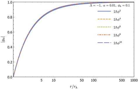
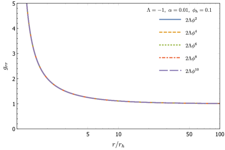
Figure 1: The metric components $|g_{tt}|$ (left plot) and $g_{rr}$ (right plot) in terms of the radial coordinate $r$, for $f(\phi)=\alpha e^{\phi}$ and a variety of potentials $V(\phi)$ (with $\Lambda=-1$).

We will first discuss the case of an exponential coupling function, $f(\phi)=\alpha e^{\phi}$. The solutions for the metric functions $e^{A(r)}$ and $e^{B(r)}$ are depicted in the left and right plot of Fig. 1, respectively, for a variety of forms of the scalar-field potential $V(\phi)$. We observe the anticipated behaviour near the black-hole horizon, with $e^{A(r)}$ vanishing and $e^{B(r)}$ diverging. At large distances, the gravitational background approaches the Minkowski spacetime. Therefore, the asymptotic forms of the metric functions read

$$A(r)\simeq-\frac{2M}{r}+{\cal O}\left(\frac{1}{r^{2}}\right)\,,\qquad B(r)\simeq\frac{2M}{r}+{\cal O}\left(\frac{1}{r^{2}}\right)\,,$$ (42)

from which we may easily obtain the mass $M$ of the black hole. The solutions presented correspond to the particular values $\Lambda=-1$ (in units of $r_{h}^{-2}$), $\alpha=0.01$ (in units of $r_{h}^{2}$) and $\phi_{h}=0.1$, however, the observed behaviour is typical for a large range of values we have used. We note that the behaviour of the metric functions both at small and large distances from the black-hole horizon is in fact independent of the form of the scalar-field potential $V(\phi)$, as Fig. 1 clearly depicts . We would like to stress that the asymptotically-flat behaviour of the $g_{rr}$ metric component at radial infinity follows naturally by solving the field equations from the horizon outwards and without imposing any condition at large distances. The $g_{tt}$ component also approaches naturally a finite, constant value, and the boundary condition $g_{tt}\rightarrow-1$, as $r\rightarrow\infty$, is imposed in order to determine the parameter $a_{1}$ which otherwise remains arbitrary.

The spacetime remains everywhere regular as this may be seen from the profile of the curvature-invariant GB term depicted in the left plot of Fig. 2. As expected, the GB term assumes its maximum value near the black-hole horizon, where the curvature is maximum, and quickly decreases eventually vanishing far way from the horizon. Once again, the exact form of the scalar-field potential $V(\phi)$ does not affect the profile of the gravitational GB term. The regularity of the spacetime is also reflected in the finiteness of all components of the energy-momentum tensor presented on the right plot of Fig. 2. Here, the indicative case of the quartic potential, $V(\phi)=\phi^{4}$, is presented, however, the observed profile remains unaffected as the form of $V(\phi)$ varies. We may clearly see the characteristic behaviour caused by the presence of the GB in the theory: the radial pressure $p=T^{r}_{\;\,r}$ is positive near the horizon while the energy density $\rho=-T^{t}_{\;\,t}$ is negative – both these features cause the evasion of the scalar no-hair theorems [13, 39] and the emergence of regular black-hole solutions with scalar hair. The depicted profiles of $T^{\mu}_{\;\,\nu}$ also reveal the asymptotic flatness of spacetime as all components assume a zero value away from the black-hole horizon.

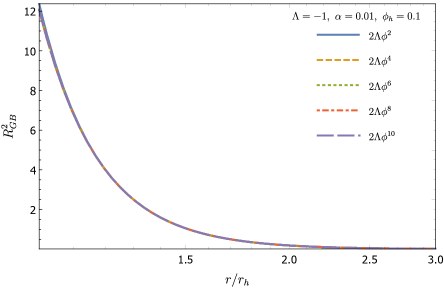
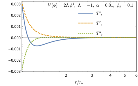
Figure 2: The Gauss-Bonnet term $R^{2}_{GB}$ for a variety of potentials $V(\phi)$ (left plot)  and the energy-momentum tensor $T^{\mu}_{\;\,\nu}$ (right plot) for the indicative case of the quartic potential, $V(\phi)=\phi^{4}$, in terms of the radial coordinate $r$, for $f(\phi)=\alpha e^{\phi}$ and $\Lambda=-1$.

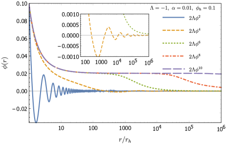
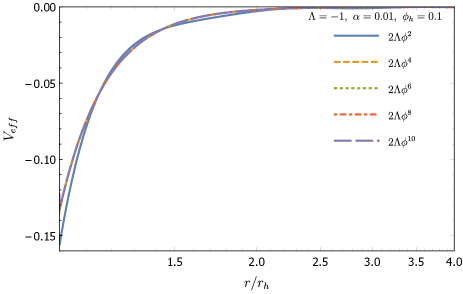
Figure 3: The scalar field (left plot) and its effective potential $V_{eff}$ (right plot) in terms of the radial coordinate $r$, for $f(\phi)=\alpha e^{\phi}$ and various forms of $V(\phi)$ (with $\Lambda=-1$).

Let us now turn to the profile of the scalar field which supports the aforementioned behaviour of the energy-momentum tensor. This is depicted in the left plot of Fig. 3, for a variety of forms of its potential $V(\phi)$. As demonstrated in Section 3, the scalar field is regular near the black-hole horizon independently of the form of its potential. However, the subsequent evolution does strongly depend on the particular form of $V(\phi)$. We observe that, despite the negative sign of $\Lambda$, the profile of the scalar field remains finite in the entire radial regime. For all of the forms of $V(\phi)$ employed, the scalar field decreases at the near-horizon regime and reduces to a vanishing value at asymptotic infinity. Once again, no boundary condition is imposed at large distances on the scalar field, which naturally approaches a zero value. This is supported also by the behaviour of the effective potential of the scalar field defined as

$$V_{eff}=-f(\phi)\,R^{2}_{GB}+2\Lambda\,V(\phi)\,,$$ (43)

the value of which is presented in the right plot of Fig. 3. For all forms of $V(\phi)$, the effective potential adopts its maximum value near the black hole horizon, where it supports a non-trivial scalar field, while it decays to zero at asymptotic infinity leading to a trivial scalar field there. The asymptotic behaviour of the scalar field is difficult to obtain in an analytic way; employing the asymptotic forms (42) of the metric functions, the scalar-field equation (14) takes the form

$$r\phi^{\prime\prime}+2\phi^{\prime}-2r\Lambda\frac{dV}{d\phi}=0\,.$$ (44)

For $V(\phi)=0$, the above equation leads to the solution (35), which is indeed the asymptotic behaviour of a scalar field possessing only a coupling to the GB term and no potential [39]. For $V(\phi)=\phi^{2}$ and $\Lambda=m^{2}/2$, the solution is given by Eq. (37) describing the asymptotic form of a massive scalar field [90]. For the case with $V(\phi)=\phi^{2}$ and $\Lambda=-m^{2}/2$ that we consider here, the solution of Eq. (44) takes the form

$$\phi(r)\simeq\frac{1}{r}\,[C_{1}\cos(mr)+C_{2}\,\sin(mr)]\,.$$ (45)

The above solution justifies the oscillatory behaviour clearly observed in the lower curve of the left plot of Fig. 3, which corresponds to this case. Unfortunately, Eq. (44) cannot be analytically solved for any of the other forms of the scalar potential $V(\phi)$ that we study in this work. The similarity in the profile of the effective potential but also the observed behaviour of the scalar-field curves, depicted in Fig. 3 for $V(\phi)=\phi^{2n}$, imply that the scalar field decreases asymptotically to zero in an oscillatory way also for the cases with $n>1$; however, as $n$ increases, the frequency of the oscillations is strongly damped and the asymptotic vanishing value is reached at an increasingly larger distance.

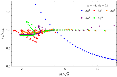
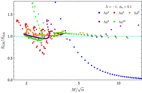
Figure 4: The horizon radius $r_{h}$ (left plot) and entropy $S_{GB}$ (right plot) normalised with respect to the corresponding Schwarzschild values, for $f(\phi)=\alpha e^{\phi}$ and different forms of $V(\phi)$ (with $\Lambda<0$).

Although this may be true, there seem to be some fundamental differences between the GB black-hole solutions where the scalar field possesses a quadratic potential and the solutions where the scalar field has a higher-power potential. To see this, in Fig. 4, we plot the horizon radius and the entropy of the corresponding black-hole solutions in terms of their mass $M$. These quantities are normalised to the corresponding Schwarzschild values, $r_{Sch}=2M$ and $S_{Sch}=4\pi M^{2}$, for easy comparison. All solutions for $V(\phi)=\phi^{2n}$ with $n>1$ exhibit the existence of multiple branches with their horizon radius and entropy being smaller or larger than the corresponding Schwarzschild values depending on the mass range and value of the power $n$. On the other hand, the quadratic case allows only one branch, which crosses the horizontal line, marking the equality of $r_{h}$ and $S_{GB}$ with the Schwarzschild values, at only one point: black holes with masses below that point have a horizon radius larger than the corresponding Schwarzschild solution and are also more thermodynamically stable. For all forms of the scalar potential, our numerical analysis has revealed the existence of an upper bound on the coupling parameter $\alpha$, which then translates to a lower bound for the black-hole mass $M$, a feature common for all GB black holes [13, 39, 160].

Another distinctive feature of the case with a negative quadratic potential is the behaviour of the black-hole solutions in the limit of large mass, a feature that distinguishes this case both from the ordinary massive case and from the case with a higher-power potential. From Fig. 4, we observe that, as the mass of the black-hole solution increases, the horizon radius and entropy for the case with $V(\phi)=\phi^{2}$ decrease reaching eventually a very small value. Thus, in the limit of large mass, a branch of massive, ultra-compact black holes seems to emerge. In contrast, for all other forms of the scalar-field potential, this branch of solutions is absent since the horizon radius and entropy of the corresponding solutions approach, in the limit of large mass, values which are very close to the Schwarzschild ones. In the ordinary massive case [90], the GB black holes also approach the Schwarzschild solution in the large-mass limit. We consider the emergence of this ultra-compact family of black holes as a rather interesting feature of the theory, therefore, in the next subsection we study in greater detail the case with a negative quadratic potential.

5.2 Exponential Coupling Function with a Quadratic Potential

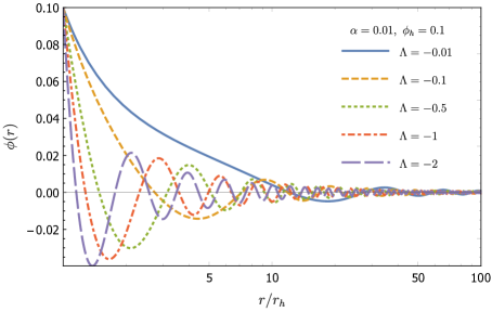
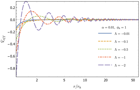
Figure 5: The scalar field $\phi$ (left plot) and its source term $\dot{V}_{eff}$ (right plot) in terms of the radial coordinate $r$, for $f(\phi)=\alpha e^{\phi}$ and $V(\phi)=\phi^{2}$ (with $\Lambda<0$).

If we focus on the EsGB theory with an exponential coupling function and a negative quadratic potential, the decisive parameter of the theory is the coupling parameter $\Lambda$. The form of the metric functions $A(r)$ and $B(r)$ are not significantly affected as $\Lambda$ varies, and they are still accurately described by the profiles depicted in Fig. 1. However, $\Lambda$ strongly affects the solution for the scalar field: as may be clearly seen from the left plot of Fig. 5, the parameter $\Lambda$ affects both the rate of decrease of the scalar field near the black-hole horizon and the frequency of the oscillatory phase as the asymptotic solution at infinity is approached. These dependences are also supported by Eq. (27) and Eq. (45), where $m=\sqrt{2|\Lambda|}$, respectively. We note that both of these quantities increase with $\Lambda$. The same holds for the source term $\dot{V}_{eff}$, which appears in the scalar-field equation (4) and determines the profile of the scalar field; this is depicted in the right plot of Fig. 5 for various values of $\Lambda$.

Finally, as expected, the same oscillatory behaviour is observed also in the components of the energy-momentum tensor, and becomes more prominent as $\Lambda$ increases. In Fig. 6, we display all three $T^{\mu}_{\;\,\nu}$ components for $\Lambda=-0.5$ (left plot) and $\Lambda=-2$ (right plot) with all the other parameters fixed. The overall behaviour noted in Fig. 2 is observed also here, with all components remaining finite and approaching zero values at infinity. In addition, we note that, as $\Lambda$ increases, an oscillatory phase appears in all components and is preserved until the asymptotic regime at infinity is reached.

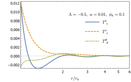
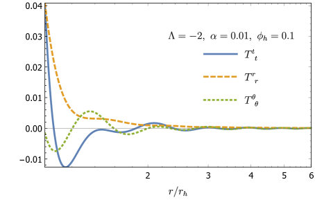
Figure 6: The energy-momentum tensor $T^{\mu}_{\;\,\nu}$ components for $f(\phi)=\alpha e^{\phi}$ and $V(\phi)=\phi^{2}$, and two different values of $\Lambda$, namely $\Lambda=-0.5$ (left plot) and $\Lambda=-2$ (right plot).

In Fig. 7, we plot again the horizon radius $r_{h}$ (left plot) and entropy $S_{GB}$ (right plot) normalised with respect to the corresponding Schwarzschild values, for solutions obtained for $f(\phi)=\alpha e^{\phi}$, $V(\phi)=\phi^{2}$ and various negative values of the parameter $\Lambda$. The case with $\Lambda=0$ corresponding to the asymptotically-flat dilatonic GB black holes with no potential [13, 39] is also shown for comparison. From the left plot of Fig. 7, we observe that whereas the dilatonic black holes are always smaller than the corresponding Schwarzschild black holes, the black-hole solutions with a negative quadratic potential may be either smaller, equal or larger than the Schwarzschild solution with respect to their horizon values. The same holds for the entropy of these solutions, shown in the right plot, with the ones being larger in size than the Schwarzschild radius being also more thermodynamically stable. The new feature emerging from these plots is that, also for the negative quadratic potential, branches of solutions with the same mass $M$ but with different horizon radii and entropies appear for certain regimes of the $\Lambda$ parameter.

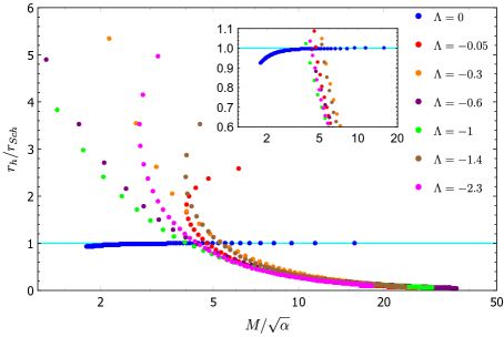
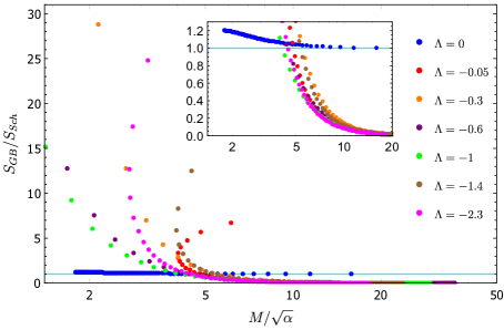
Figure 7: The horizon radius $r_{h}$ (left plot) and entropy $S_{GB}$ (right plot) normalised with respect to the corresponding Schwarzschild values, for $f(\phi)=\alpha e^{\phi}$, $V(\phi)=\phi^{2}$ and various values of $\Lambda<0$. The blue dots correspond to the dilatonic black holes with no potential ($\Lambda=0$).

The branch of the massive ultra-compact GB black holes is also present for every non-vanishing, negative value of the coupling parameter $\Lambda$. In fact, the exact value of $\Lambda$ determines the value of $M$ where this branch terminates. As the mass $M$ increases, the horizon radius gets smaller and its entropy decreases to a very small value. The question emerges of whether the end point is indeed a black hole with a small but non-vanishing horizon radius or perhaps a naked singularity. To investigate this, in Fig. 8 we plot the values of the GB term at the location of the horizon (multiplied by $f(\phi_{h})$ for scaling purposes) in terms of the black-hole mass $M$ of the solutions. The case of the dilatonic black holes with $\Lambda=0$ is again shown for comparison. We observe that, in the presence of a negative potential, a reversal takes place in the behaviour of the GB term: for $\Lambda=0$, it is the low-mass GB black-hole solutions that are the most compact, and therefore create the most curved background around them; for $\Lambda<0$, on the other hand, it is the black-hole solutions near the end point of the branch of ultra-compact objects, i.e. the black holes with the smallest horizon radius and the largest mass, that naturally create the most curved background. Although the GB term reaches a large value, it never becomes infinite – the solutions at the end of the branch have a GB term at their horizon which is comparable to the one for a dilatonic black hole with no potential. This signifies the fact that the horizon radius, although very small, remains in fact non-vanishing and therefore these massive, ultra-compact objects are extremely small-sized black holes. The existence of a minimum horizon radius is also supported by the constraint $r_{h}>-2\dot{f}_{h}\phi_{h}$ discussed in Section 3. As follows from the left plots of Figs. 3 and 5, the quantity $\phi^{\prime}_{h}$ is always negative while, for all of our choices, $\dot{f}>0$; as a result, the aforementioned inequality does impose a lower bound on the horizon value of our black-hole solutions. For a quadratic potential, this lower bound corresponds to the end point of the branch of massive, ultra-compact black holes.

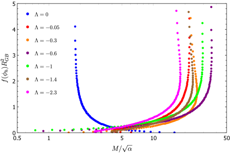
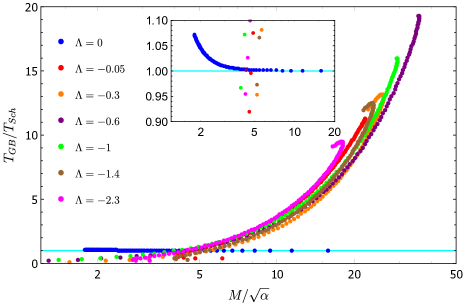
Figure 8: The combination $f(\phi)\,R^{2}_{GB}$ at the horizon radius (left plot) and the temperature (right plot) in terms of the mass $M$, for $f(\phi)=\alpha e^{\phi}$, $V(\phi)=\phi^{2}$ and various values of $\Lambda<0$. The blue dots correspond again to the dilatonic black holes with no potential ($\Lambda=0$).

In the right plot of Fig. 8, we finally present the temperature of the black-hole solutions, found in the case of an exponential coupling functions and a negative quadratic potential, in terms of the mass and for different values of $\Lambda$. We observe that the temperature of all the solutions belonging to the group of light but large black holes have a temperature smaller than the Schwarzschild one. In contrast, all solutions belonging to the group of massive, compact black holes have a temperature larger than the Schwarzschild value, which increases as we approach the end point of the branch of ultra-compact solutions. Therefore, the thermodynamically more stable solutions, from the point-of-view of the entropy, have a small temperature while the less stable have a large temperature. In contrast, the behaviour of the temperature depends only mildly on the coupling parameter $\Lambda$.

5.3 Different Coupling Functions with a Quadratic Potential

We would now like to investigate whether the emergence of the aforementioned black-hole solutions is restricted only in the case of the exponential coupling function between the scalar field and the GB term or is a generic feature of the class of EsGB theories. We have therefore considered a variety of coupling functions, mainly odd and even polynomial functions of the form $f(\phi)=\alpha\phi^{\ell}$, with $\ell$ a positive integer. We have also kept the scalar quadratic potential in order to investigate whether both large and small-sized black holes continue to emerge.

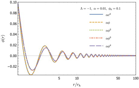
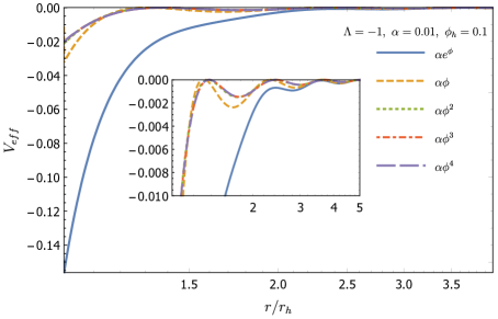
Figure 9: The scalar field (left plot) and its effective potential $V_{eff}$ (right plot) in terms of the radial coordinate $r$, for $V(\phi)=\phi^{2}$ (with $\Lambda=-1$) and a variety of coupling functions $f(\phi)$.

According to our analysis, classes of black holes similar to the ones presented in section 5.2 emerge in every single case. The solutions for the metric functions are given by curves identical to the ones in Fig. 1 for every coupling function - as in the case with no scalar potential [39, 160], the exact form of $f(\phi)$ is of minor importance for the solution of the gravitational background. The solution for the scalar field is more strongly affected by the form of $f(\phi)$, as can be seen in the left plot of Fig. 9. In fact, there seems to be a common behaviour of the solutions for the scalar field for the coupling functions $f(\phi)=\alpha e^{\phi}$ and $f(\phi)=\alpha\phi$ and another one for all higher polynomials $f(\phi)=\alpha\phi^{\ell}$, with $\ell>1$. In all cases, the scalar field is finite and oscillates towards a vanishing value at asymptotic infinity. As in the case of the exponential coupling function, also here, the value of the coupling parameter $\Lambda$ affects the near-horizon slope and the frequency of oscillations appearing in the curve of the scalar field. It also affects in a similar way the effective potential of the scalar field (whose form for a fixed value of $\Lambda$ is shown in the right plot of Fig. 9) and the energy-momentum tensor components, therefore, we refrain from presenting additional plots here.

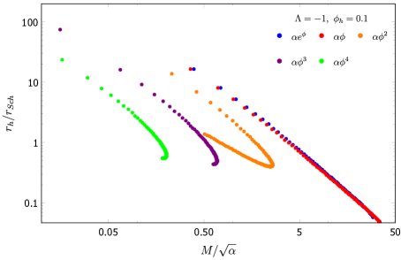
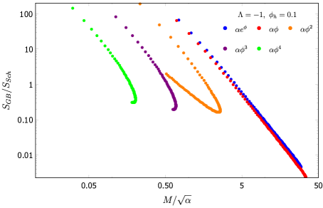
Figure 10: The horizon radius $r_{h}$ (left plot) and entropy $S_{GB}$ (right plot) normalised with respect to the corresponding Schwarzschild values, for $V(\phi)=\phi^{2}$ (with $\Lambda=-1$) and a variety of coupling functions $f(\phi)$.

The horizon radius and entropy of the black-hole solutions obtained for different forms of the coupling function $f(\phi)$, normalised again to the corresponding Schwarzschild values, are presented in Fig. 10. For a quadratic scalar potential, we observe that all classes of solutions extend between a maximum and a minimum horizon radius, which in turn corresponds to a minimum and a maximum mass for the black holes. The subgroup of black holes with a horizon radius larger than the Schwarzschild solution have also a larger entropy, and thus they are more thermodynamically stable. Independently of the form of the coupling function, the smallest in mass GB black holes with a negative quadratic potential are typically 10 times larger than the corresponding Schwarzschild solution, and have at least two orders of magnitude larger entropy.

The subgroup of the more massive black holes, on the other hand, terminates for each coupling function at a different maximum value of the mass, or at a different minimum value of the horizon radius, as the bound $r_{h}>-2\dot{f}_{h}\phi^{\prime}_{h}$ dictates. The solutions for the exponential and linear coupling functions have the largest upper value for the mass and the smallest horizon radius of all, with the latter being approximately the 1/20 of the horizon radius of the Schwarzschild solution with the same mass. In contrast, as the integer $m$ in the form of the coupling function increases, the maximum mass decreases and the minimum horizon radius increases. Since the small-sized black holes are smaller in entropy compared to the Schwarzschild solution, they are also less thermodynamically stable. According to the right plot of Fig. 10, the dilatonic and ‘linear’ GB ultra-compact black holes have two orders of magnitude smaller entropy than the Schwarzschild solution. This is the same difference in entropy as the one between the small-mass GB black holes and the Schwarzschild solution. In other words, the ultra-compact GB black holes are less thermodynamically stable compared to the Schwarzschild solution as much as the Schwarzschild solution is less stable compared to the small-mass GB black holes. On the other hand, the ‘quadratic’ and ‘higher’ GB black holes have approximately the 1/4 of the entropy of the Schwarzschild solution. This makes them much more thermodynamically stable than their dilatonic and ‘linear’ analogues but their compactness is limited being typically only half in size compared to the Schwarzschild solution.

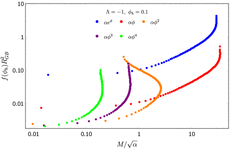
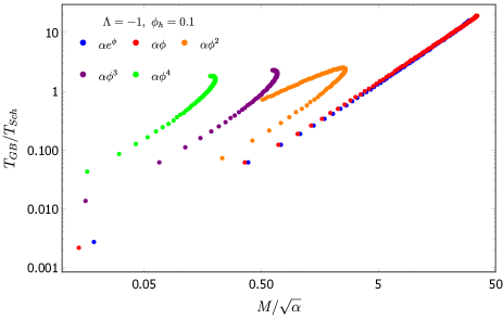
Figure 11: The combination $f(\phi)\,R^{2}_{GB}$ at the horizon radius (left plot) and the temperature (right plot) in terms of the mass $M$, for $V(\phi)=\phi^{2}$ (and $\Lambda=-1$) and various forms of the coupling function $f(\phi)$.

In Fig. 11 (left plot), we depict again the combination $f(\phi)\,R^{2}_{GB}$ at the horizon of the black-hole solutions, in terms of their mass $M$, for the quadratic negative potential and for various forms of the coupling function. We observe again that the GB term remains finite even close to the end point of the branch of the ultra-compact solutions. In accordance with the previous findings, the curvature of spacetime is stronger around the small-sized, massive black holes obtained for the exponential and linear coupling functions, which constitute the most compact objects found in this theory. Finally, in the right plot of Fig. 11, we present the temperature of the black-hole solutions, found for a negative quadratic potential and various coupling functions. The same behaviour found in the case of the exponential coupling function is also observed here: the light but large black holes have a temperature smaller than the Schwarzschild one while the massive, compact black holes have a temperature larger than the Schwarzschild value. Again, it is the exponential and linear coupling functions which produce the solutions with the largest values of the temperature. In the opposite limit of small mass, it is also the same coupling functions that produce the smallest values of the temperature and support the most thermodynamically stable solutions.

6 Conclusions

In this work, we have focused on the study of the EsGB theory where the scalar field possesses also a self-interacting potential. This potential was considered to be negative and thus to have the opposite sign in the action compared to a traditional self-interacting term. This choice was motivated by our desire to investigate whether this theory, which yielded a plethora of novel black-hole solutions with a non-trivial scalar field in the presence of a negative cosmological constant [160], could still support similar types of solutions in the more realistic case where the constant negative distribution of energy is replaced by a negative field potential. To this end, we have considered a variety of forms for both the coupling function between the scalar field and the GB term and for the scalar-field potential, and looked for static, spherically-symmetric, regular black holes with a non-trivial scalar field.

We first performed an analytic study of the field equations and demonstrated that, independently of the forms of the scalar-GB coupling function and of the scalar potential, an asymptotic solution describing a black-hole horizon with a regular scalar field always emerges. The particular choices for these two functions do not significantly affect the form of the gravitational background either close to or far away from the black-hole horizon. The field equations lead naturally to asymptotically-flat families of solutions which are everywhere regular, as the profile of the scale-invariant GB term reveals. The solution for the scalar field does depend on the assumed form of its potential but it always describes a regular field approaching a vanishing value at asymptotic infinity. All components of the energy-momentum tensor also remain finite for every choice of the scalar potential and coupling function, and tend asymptotically to zero values in agreement with the asymptotic flatness of the solutions. The effective potential of the scalar field receives contributions from both the GB coupling and the negative potential, however, both contributions remain bounded and both vanish at large distances.

Using the case of the exponential scalar-GB coupling function as a prototype, we varied the form of the scalar potential and studied the properties of the black-hole solutions obtained, namely the horizon radius, the entropy and the temperature. We have found a distinctly different behaviour of the parameters of the black holes obtained for either $V(\phi)=\phi^{2}$ or for $V(\phi)=\phi^{2n}$, with $n>1$. In the latter case, branches of solutions, either smaller or larger than the Schwarzschild solution depending on their mass and value of $n$, were found; these solutions were characterised by a minimum mass and approached the properties of the Schwarzschild solution in the limit of large mass, as all previously found GB black holes [13, 39, 160]. In the former case, however, of a negative quadratic potential, the solutions are divided in two subgroups: the first subgroup comprises the small-mass GB black holes which all have a larger horizon radius, a larger entropy and a smaller temperature compared to the Schwarzschild solution; the second subgroup includes the more massive black holes the horizon radius of which gets increasingly smaller as their mass increases – these solutions have also a smaller entropy and a larger temperature compared to the Schwarzschild solution. Whereas the GB black holes obtained in the case of a positive quadratic potential approach the Schwarzschild solution in the limit of large mass [90], the GB solutions supported by a negative quadratic potential exhibit a regime of very massive but ultra-compact subgroup of black holes.

The same behaviour is observed when the coupling function between the scalar field and the GB term assumes a polynomial function, either even or odd, of the scalar field. The only differences appear in the values of the minimum and maximum values of the horizon radius, or correspondingly the mass, of the black-hole solutions obtained in each case. In all cases, however, the spacetime remains regular even around the massive, ultra-compact solutions. According to our results, the most compact black holes emerge for either the exponential (dilatonic) or linear form of the coupling function with the smallest horizon radius being approximately the 1/20 of the horizon radius of a Schwarzschild black hole with exactly the same mass. These objects have only the 1/100 of the entropy of the Schwarzschild solution, while the Schwarzschild solution has again only the 1/100 of the entropy of the largest (and less massive) GB black holes in the theory.

It is worth stressing again the large differences found between the results derived in this work and those found in the case of a negative cosmological constant [160], as this was our main motivation. In the latter case, the constant, negative $\Lambda$ term worked together with the GB term in order to create a branch of black holes which started from the Schwarzschild solution, in the limit of large mass, and gave increasingly smaller black holes (both in terms of the mass and the horizon radius) until the point of minimum mass, and minimum horizon radius, was reached. When the negative cosmological constant is replaced by a negative field potential – different from quadratic – the existence of a branch of solutions extending from the Schwarzschild limit down to a minimum-mass GB black-hole is still observed; however, the horizon radius may be larger or smaller than the Schwarzschild value depending on the particular value of the mass of the black hole. When specifically the negative quadratic potential is considered, we have the appearance of the two distinct subgroups of light but large black holes (as in the case of a positive quadratic potential [90]) and the massive but ultra-compact ones. The reversal in the behaviour of the GB term in this case is also interesting: whereas in the asymptotically-flat [39] and asymptotically AdS [160] cases, the GB takes its largest value around the black holes with the minimum mass, now it is the most massive black holes which create the most curved gravitational background around them; the reason for that is clearly the fact that these are now the most compact objects in the theory.

The above solutions owe their existence to the synergy of the GB term with the negative scalar potential. Black holes emerging in the theory of a minimally-coupled scalar field with a negative potential would be most likely considered as unnatural objects – indeed, to our knowledge, no such black-hole solutions have been derived or studied. In our analysis, we have demonstrated that, in the presence of the GB term, the negative potential does not comprise a source of any irregular or destabilising effects in our solutions. Both the distribution of energy and the spacetime remain finite outside the black-hole horizon, and support solutions for the scalar field which are always bounded and naturally die out at large distances. The negativity of the potential may have implications on the stability of the solutions under perturbations. Although the form of the entropy hints towards the fact that a large number of them may in fact be stable from the thermodynamical point of view, this remains to be investigated. Even if a subclass of our solutions turns out to be unstable, their emergence for a finite amount of time may be in fact associated with interesting phenomena especially in the strong gravitational-field limit where quadratic terms, such as the GB, are expected to be important.

Acknowledgments We would like to thank Georgios Antoniou for valuable discussions during the early stages of this work. This research is implemented through the Operational Program “Human Resources Development, Education and Lifelong Learning” and is co-financed by the European Union (European Social Fund) and Greek national funds (MIS code: 5006022).

Appendix A Set of Differential Equations

Here, we display the explicit expressions of the coefficients $P$, $Q$ and $S$ which appear in the system of differential equations (18)-(19). For notational simplicity, in these expressions we have eliminated, via Eq. (17), $B^{\prime}$, which involves $A^{\prime\prime}$ and $\phi^{\prime\prime}$, but retained $e^{B}$. They are:

$$P =-128e^{4B}\Lambda^{2}r^{3}V^{2}\dot{f}\left(rA^{\prime}+2e^{B}-2\right)+16A^{\prime 3}\dot{f}\bigl{[}-2e^{B}\left(-14e^{B}+3e^{2B}+19\right)r\dot{f}\phi^{\prime}$$

$$+8\left(-8e^{B}+3e^{2B}+9\right)\dot{f}^{2}\phi^{\prime 2}-e^{2B}\left(3e^{B}-5\right)r^{2}\bigr{]}+4e^{B}A^{\prime 2}\Big{\{}e^{B}r\dot{f}\Bigl{[}\left(5e^{B}-19\right)r^{2}\phi^{\prime 2}$$

$$+12\left(e^{B}-1\right)^{2}\Bigr{]}-4\dot{f}^{2}\phi^{\prime}\Big{[}\left(9e^{B}-17\right)r^{2}\phi^{\prime 2}+8\left(e^{B}-1\right)^{2}\Big{]}+e^{2B}r^{4}\phi^{\prime}\Big{\}}$$

$$+4e^{2B}2\,V\Lambda\Bigl{\{}-e^{2B}r^{3}(-2+rA^{\prime})\phi^{\prime}-16A^{\prime}\dot{f}^{2}\phi^{\prime}\left[6(3-4e^{B}+e^{2B})+(-5+e^{B})rA^{\prime}\right]$$

$$+4e^{B}\dot{f}\Bigl{[}-3r^{2}A^{\prime 2}(1+e^{B})+4\Bigl{(}4(-1+e^{B})^{2}-r^{2}\phi^{\prime 2}\Bigr{)}+2rA^{\prime}(3-3e^{B}+r^{2}\phi^{\prime 2})\Bigr{]}\Bigr{\}}$$

$$-2e^{2B}r\phi^{\prime}\Bigl{\{}8\dot{f}\Big{[}4r\Lambda\dot{V}e^{B}(-1+e^{B})-\phi^{\prime}\Big{(}4e^{B}(-1+e^{B})+r^{2}\phi^{\prime 2}(-2+e^{B})\Bigr{)}\Big{]}$$

$$-4re^{B}(-1+e^{B})-r\phi^{\prime 2}\Bigl{[}r^{2}e^{B}-16\ddot{f}(-1+e^{B})\Bigr{]}\Bigr{\}}-A^{\prime}e^{B}\Bigl{\{}-32r\dot{f}^{2}\phi^{2}\Big{[}8r\Lambda\dot{V}e^{2B}$$

$$-\phi^{\prime}(9-4e^{B}+3e^{2B})\Bigr{]}-r^{3}\phi^{\prime}e^{B}\Big{[}4e^{B}(1+e^{B})-\phi^{\prime 2}\Bigl{(}r^{2}e^{B}+16\ddot{f}(1+e^{B})\Big{)}\Big{]}$$

$$+8e^{B}\dot{f}\Big{[}4(-1+e^{B})^{2}+4r^{3}\Lambda\dot{V}\phi^{\prime}e^{B}(1+e^{B})+r^{2}\phi^{\prime 2}(-7+3e^{B})-2\phi^{\prime 4}(r^{4}+8r^{2}\ddot{f})\Big{]}\Big{\}},$$ (A.1)

$$Q =2304A^{\prime}\dot{f}^{2}\ddot{f}\phi^{\prime 4}-1152A^{\prime 2}\dot{f}^{3}\phi^{\prime 3}+e^{B}\Big{(}-144r^{2}A^{\prime}\dot{f}^{2}\phi^{\prime 4}+672rA^{\prime 2}\dot{f}^{2}\phi^{\prime 2}+768A^{\prime 2}\dot{f}^{3}\phi^{\prime 3}$$

$$-384A^{\prime}\dot{f}^{2}\phi^{\prime 2}-1024rA^{\prime}\dot{f}\ddot{f}\phi^{\prime 3}-3584A^{\prime}\dot{f}^{2}\ddot{f}\phi^{\prime 4}+480r\dot{f}^{2}\phi^{\prime 4}+64r^{2}\dot{f}\ddot{f}\phi^{\prime 5}-640\dot{f}\ddot{f}\phi^{\prime 3}\Big{)}$$

$$+e^{2B}\Big{(}128r^{2}A^{\prime}\ddot{f}\phi^{\prime 2}+52r^{3}A^{\prime}\dot{f}\phi^{\prime 3}+80r^{2}A^{\prime}\dot{f}^{2}\phi^{\prime 4}-128r^{2}A^{\prime 2}\dot{f}\phi^{\prime}-576\Lambda r^{2}VA^{\prime}\dot{f}^{2}\phi^{\prime 2}$$

$$-320rA^{\prime 2}\dot{f}^{2}\phi^{\prime 2}+176rA^{\prime}\dot{f}\phi^{\prime}-128A^{\prime 2}\dot{f}^{3}\phi^{\prime 3}+640A^{\prime}\dot{f}^{2}\phi^{\prime 2}+1280rA^{\prime}\dot{f}\ddot{f}\phi^{\prime 3}+1280A^{\prime}\dot{f}^{2}\ddot{f}\phi^{\prime 4}$$

$$-16r^{3}\ddot{f}\phi^{\prime 4}+128r\ddot{f}\phi^{\prime 2}-4r^{4}\dot{f}\phi^{\prime 5}-152r^{2}\dot{f}\phi^{\prime 3}-384\Lambda r^{2}\dot{f}^{2}\phi^{\prime 3}\dot{V}-256r\dot{f}^{2}\phi^{\prime 4}+384\Lambda rV\dot{f}^{2}\phi^{\prime 2}$$

$$+160\dot{f}\phi^{\prime}-64r^{2}\dot{f}\ddot{f}\phi^{\prime 5}-512\Lambda r^{2}V\dot{f}\ddot{f}\phi^{\prime 3}+1280\dot{f}\ddot{f}\phi^{\prime 3}\Big{]}+e^{3B}\Big{[}-128r^{2}A^{\prime}\ddot{f}\phi^{\prime 2}-12r^{3}A^{\prime}\dot{f}\phi^{\prime 3}$$

$$+208\Lambda r^{3}VA^{\prime}\dot{f}\phi^{\prime}+32r^{2}A^{\prime 2}\dot{f}\phi^{\prime}+320\Lambda r^{2}VA^{\prime}\dot{f}^{2}\phi^{\prime 2}+32rA^{\prime 2}\dot{f}^{\prime 2}\phi^{\prime 2}-224rA^{\prime}\dot{f}\phi^{\prime}$$

$$-256A^{\prime}\dot{f}^{2}\phi^{\prime 2}-256rA^{\prime}\dot{f}\ddot{f}\phi^{\prime 3}-6r^{4}A^{\prime}\phi^{\prime 2}+8r^{3}A^{\prime 2}-24r^{2}A^{\prime}+16r^{3}\ddot{f}\phi^{\prime 4}+128\Lambda r^{3}V\ddot{f}\phi^{\prime 2}$$

$$-256r\ddot{f}\phi^{\prime 2}+16\Lambda r^{4}V\dot{f}\phi^{\prime 3}+160\Lambda r^{3}\dot{f}\phi^{\prime 2}\dot{V}+24r^{2}\dot{f}\phi^{\prime 3}+128\Lambda r^{2}\dot{f}^{2}\phi^{\prime 3}\dot{V}+224\Lambda r^{2}V\dot{f}\phi^{\prime}$$

$$+32r\dot{f}^{2}\phi^{\prime 4}-512\Lambda rV\dot{f}^{2}\phi^{\prime 2}-320\dot{f}\phi^{\prime}+512\Lambda r^{2}V\dot{f}\ddot{f}\phi^{\prime 3}-640\dot{f}\ddot{f}\phi^{\prime 3}+r^{5}\phi^{\prime 4}+12r^{3}\phi^{\prime 2}-32r\Big{]}$$

$$+e^{4B}\Big{[}-48\Lambda r^{3}VA^{\prime}\dot{f}\phi^{\prime}+48rA^{\prime}\dot{f}\phi^{\prime}-24\Lambda r^{4}VA^{\prime}+24r^{2}A^{\prime}-128\Lambda r^{3}V\ddot{f}\phi^{\prime 2}+128r\ddot{f}\phi^{\prime 2}$$

$$+128\Lambda^{2}r^{4}V^{2}\dot{f}\phi^{\prime}-32\Lambda r^{3}\dot{f}\phi^{\prime 2}\dot{V}-224\Lambda r^{2}V\dot{f}\phi^{\prime}+128\Lambda rV\dot{f}^{2}\phi^{\prime 2}+160\dot{f}\phi^{\prime}-4\Lambda r^{5}V\phi^{\prime 2}$$

$$-16\Lambda r^{4}\varphi^{\prime}V^{\prime}+4r^{3}\phi^{\prime 2}-64\Lambda r^{3}V+64r\Big{]}+e^{5B}\Big{[}-32\Lambda^{2}r^{5}V^{2}+64\Lambda r^{3}V-32r\Big{]},$$ (A.2)

and

$$S =2304A^{\prime}\dot{f}^{3}\phi^{\prime 2}+8e^{B}\big{(}-128rA^{\prime}\dot{f}^{2}\phi^{\prime}-448A^{\prime}\dot{f}^{3}\phi^{\prime 2}+32r^{2}\dot{f}^{2}\phi^{\prime 3}-80\dot{f}^{2}\phi^{\prime}\big{)}$$

$$+8e^{2B}\big{(}16r^{2}A^{\prime}f^{\prime}+160rA^{\prime}\dot{f}^{2}\phi^{\prime}+160A^{\prime}\dot{f}^{3}\phi^{\prime 2}-12r^{3}\dot{f}\phi^{\prime 2}-16r^{2}\dot{f}^{2}\phi^{\prime 3}-64\Lambda r^{2}V\dot{f}^{2}\phi^{\prime}$$

$$+16r\dot{f}+160\dot{f}^{2}\phi^{\prime}\big{)}+8e^{3B}\big{(}-16r^{2}A^{\prime}\dot{f}-32rA^{\prime}\dot{f}^{2}\phi^{\prime}+4r^{3}\dot{f}\phi^{\prime 2}+16\Lambda r^{3}V\dot{f}$$

$$+64\Lambda r^{2}V\dot{f}^{2}\phi^{\prime}-32r\dot{f}-80\dot{f}^{2}\phi^{\prime}+r^{4}\phi^{\prime}\big{)}+8e^{4B}\big{(}16r\dot{f}-16\Lambda r^{3}V\dot{f}\big{)}.$$ (A.3)

Appendix B Scalar Quantities

By employing the metric components of the line-element (7), one may compute the following scalar-invariant gravitational quantities:

$$R = +\frac{e^{-B}}{2r^{2}}\left(4e^{B}-4-r^{2}A^{\prime 2}+4rB^{\prime}-4rA^{\prime}+r^{2}A^{\prime}B^{\prime}-2r^{2}A^{\prime\prime}\right),$$ (B.1)

$$R_{\mu\nu}R^{\mu\nu} = +\frac{e^{-2B}}{16r^{4}}\left[8(2-2e^{B}+rA^{\prime}-rB^{\prime})^{2}+r^{2}(rA^{\prime 2}-4B^{\prime}-rA^{\prime}B^{\prime}+2rA^{\prime\prime})^{2}\right.$$ (B.2)

$$\left.+r^{2}(rA^{\prime 2}+A^{\prime}(4-rB^{\prime})+2rA^{\prime\prime})^{2}\right],$$

$$R_{\mu\nu\rho\sigma}R^{\mu\nu\rho\sigma} = +\frac{e^{-2B}}{4r^{4}}\left[r^{4}A^{\prime 4}-2r^{4}A^{\prime 3}B^{\prime}-4r^{4}A^{\prime}B^{\prime}A^{\prime\prime}+r^{2}A^{\prime 2}(8+r^{2}B^{\prime 2}+4r^{2}A^{\prime\prime})\right.$$ (B.3)

$$\left.+16(e^{B}-1)^{2}+8r^{2}B^{\prime 2}+4r^{4}A^{\prime\prime 2}\right],$$

$$R_{GB}^{2} = +\frac{2e^{-2B}}{r^{2}}\left[(e^{B}-3)A^{\prime}B^{\prime}-(e^{B}-1)A^{\prime 2}-2(e^{B}-1)A^{\prime\prime}\right].$$ (B.4)

References

- [1] K. S. Stelle, Phys. Rev. D 16 (1977) 953.
-
[2]
T. P. Sotiriou,
Lect. Notes Phys. 892 (2015) 3;
E. Berti et al., Class. Quant. Grav. 32 (2015) 243001. - [3] https://www.ligo.org/
- [4] http://www.virgo-gw.eu/
- [5] D. Lovelock, J. Math. Phys. 12, 498 (1971). doi:10.1063/1.1665613
- [6] J. D. Bekenstein, Phys. Rev. Lett. 28 (1972) 452; C. Teitelboim, Lett. Nuovo Cim. 3S2 (1972) 397.
- [7] M. S. Volkov and D. V. Galtsov, JETP Lett. 50 (1989) 346; P. Bizon, Phys. Rev. Lett. 64 (1990) 2844; B. R. Greene, S. D. Mathur and C. M. O’Neill, Phys. Rev. D 47 (1993) 2242; K. i. Maeda, T. Tachizawa, T. Torii and T. Maki, Phys. Rev. Lett. 72 (1994) 450.
- [8] H. Luckock and I. Moss, Phys. Lett. B 176 (1986) 341; S. Droz, M. Heusler and N. Straumann, Phys. Lett. B 268 (1991) 371.
- [9] J. D. Bekenstein, Annals Phys. 82 (1974) 535; Annals Phys. 91 (1975) 75.
- [10] B. Zwiebach, Phys. Lett. 156B, 315 (1985).
- [11] D. J. Gross and J. H. Sloan, Nucl. Phys. B 291, 41 (1987).
- [12] R. R. Metsaev, A. A. Tseytlin, Nucl. Phys. B293 , 385 (1987).
- [13] P. Kanti, N. E. Mavromatos, J. Rizos, K. Tamvakis and E. Winstanley, Phys. Rev. D 54 (1996) 5049; Phys. Rev. D 57 (1998) 6255.
- [14] G. W. Gibbons and K. i. Maeda, Nucl. Phys. B 298 (1988) 741.
- [15] C. G. Callan, Jr., R. C. Myers and M. J. Perry, Nucl. Phys. B 311 (1989) 673.
- [16] B. A. Campbell, M. J. Duncan, N. Kaloper and K. A. Olive, Phys. Lett. B 251 (1990) 34; B. A. Campbell, N. Kaloper and K. A. Olive, Phys. Lett. B 263 (1991) 364.
- [17] S. Mignemi and N. R. Stewart, Phys. Rev. D 47 (1993) 5259.
- [18] P. Kanti and K. Tamvakis, Phys. Rev. D 52 (1995) 3506.
- [19] T. Torii, H. Yajima and K. i. Maeda, Phys. Rev. D 55 (1997) 739.
- [20] P. Kanti and K. Tamvakis, Phys. Lett. B 392 (1997) 30; P. Kanti and E. Winstanley, Phys. Rev. D 61 (2000) 084032.
- [21] Z. K. Guo, N. Ohta and T. Torii, Prog. Theor. Phys. 120 (2008) 581; K. i. Maeda, N. Ohta and Y. Sasagawa, Phys. Rev. D 80 (2009) 104032; N. Ohta and T. Torii, Prog. Theor. Phys. 124 (2010) 207.
- [22] B. Kleihaus, J. Kunz and E. Radu, Phys. Rev. Lett. 106 (2011) 151104; B. Kleihaus, J. Kunz, S. Mojica and E. Radu, Phys. Rev. D 93 (2016) no.4, 044047.
- [23] P. Pani, C. F. B. Macedo, L. C. B. Crispino and V. Cardoso, Phys. Rev. D 84 (2011) 087501; P. Pani, E. Berti, V. Cardoso and J. Read, Phys. Rev. D 84 (2011) 104035.
- [24] C. A. R. Herdeiro and E. Radu, Phys. Rev. Lett. 112 (2014) 221101.
- [25] D. Ayzenberg and N. Yunes, Phys. Rev. D 90 (2014) 044066 Erratum: [Phys. Rev. D 91 (2015) no.6, 069905].
- [26] E. Winstanley, Lect. Notes Phys. 769 (2009) 49.
- [27] C. Charmousis, Lect. Notes Phys. 769 (2009) 299.
- [28] C. A. R. Herdeiro and E. Radu, Int. J. Mod. Phys. D 24 (2015) no.09, 1542014.
- [29] J. L. Blazquez-Salcedo et al., IAU Symp. 324 (2017) 265.
- [30] J. D. Bekenstein, Phys. Rev. D 51 (1995) no.12, R6608.
- [31] G. W. Horndeski, Int. J. Theor. Phys. 10 (1974) 363.
- [32] A. Nicolis, R. Rattazzi and E. Trincherini, Phys. Rev. D 79 (2009) 064036.
- [33] T. P. Sotiriou and V. Faraoni, Phys. Rev. Lett. 108 (2012) 081103.
- [34] L. Hui and A. Nicolis, Phys. Rev. Lett. 110 (2013) 241104.
- [35] T. P. Sotiriou and S. Y. Zhou, Phys. Rev. Lett. 112 (2014) 251102.
- [36] E. Babichev and C. Charmousis, JHEP 1408 (2014) 106.
- [37] T. P. Sotiriou and S. Y. Zhou, Phys. Rev. D 90 (2014) 124063; R. Benkel, T. P. Sotiriou and H. Witek, Class. Quant. Grav. 34 (2017) no.6, 064001; Phys. Rev. D 94 (2016) no.12, 121503.
- [38] N. Yunes and L. C. Stein, Phys. Rev. D 83 (2011) 104002.
- [39] G. Antoniou, A. Bakopoulos and P. Kanti, Phys. Rev. Lett. 120 (2018) no.13, 131102; Phys. Rev. D 97 (2018) no.8, 084037.
- [40] D. D. Doneva and S. S. Yazadjiev, Phys. Rev. Lett. 120 (2018) no.13, 131103.
- [41] H. O. Silva, J. Sakstein, L. Gualtieri, T. P. Sotiriou and E. Berti, Phys. Rev. Lett. 120 (2018) no.13, 131104.
- [42] Y. Bardoux, M. M. Caldarelli and C. Charmousis, JHEP 1205 (2012) 054.
- [43] K. Yagi, L. C. Stein, N. Yunes and T. Tanaka, Phys. Rev. D 85 (2012) 064022 Erratum: [Phys. Rev. D 93 (2016) no.2, 029902]; D. Ayzenberg, K. Yagi and N. Yunes, Phys. Rev. D 89 (2014) no.4, 044023.
- [44] C. Charmousis, T. Kolyvaris, E. Papantonopoulos and M. Tsoukalas, JHEP 1407 (2014) 085.
- [45] F. Correa, M. Hassaine and J. Oliva, Phys. Rev. D 89 (2014) no.12, 124005.
- [46] S. R. Dolan, S. Ponglertsakul and E. Winstanley, Phys. Rev. D 92 (2015) no.12, 124047.
- [47] J. L. Blazquez-Salcedo, C. F. B. Macedo, V. Cardoso, V. Ferrari, L. Gualtieri, F. S. Khoo, J. Kunz and P. Pani, Phys. Rev. D 94 (2016) no.10, 104024.
- [48] S. Bhattacharya and S. Chakraborty, Phys. Rev. D 95 (2017) no.4, 044037; I. Banerjee, S. Chakraborty and S. SenGupta, Phys. Rev. D 96 (2017) no.8, 084035.
- [49] D. D. Doneva and S. S. Yazadjiev, JCAP 1804 (2018) no.04, 011.
- [50] H. Motohashi and M. Minamitsuji, Phys. Lett. B 781 (2018) 728; Phys. Rev. D 98 (2018) no.8, 084027.
- [51] C. A. R. Herdeiro, E. Radu, N. Sanchis-Gual and J. A. Font, Phys. Rev. Lett. 121 (2018) no.10, 101102; T. Delsate, C. Herdeiro and E. Radu, Phys. Lett. B 787 (2018) 8; Y. Brihaye, C. Herdeiro and E. Radu, Phys. Lett. B 788 (2019) 295.
- [52] D. D. Doneva, S. Kiorpelidi, P. G. Nedkova, E. Papantonopoulos and S. S. Yazadjiev, Phys. Rev. D 98 (2018) no.10, 104056.
- [53] M. Butler, A. M. Ghezelbash, E. Massaeli and M. Motaharfar, arXiv:1808.03217 [hep-th].
- [54] B. Danila, T. Harko, F. S. N. Lobo and M. K. Mak, arXiv:1811.02742 [gr-qc].
- [55] M. M. Stetsko, arXiv:1811.05030 [hep-th].
- [56] O. J. Tattersall, P. G. Ferreira and M. Lagos, Phys. Rev. D 97 (2018) no.8, 084005.
- [57] S. Mukherjee and S. Chakraborty, Phys. Rev. D 97 (2018) no.12, 124007.
- [58] S. Chakrabarti, Eur. Phys. J. C 78 (2018) no.4, 296.
- [59] E. Berti, K. Yagi and N. Yunes, Gen. Rel. Grav. 50 (2018) no.4, 46.
- [60] Y. Brihaye and B. Hartmann, Class. Quant. Grav. 35 (2018) no.17, 175008.
- [61] K. Prabhu and L. C. Stein, Phys. Rev. D 98 (2018) no.2, 021503.
- [62] Y. S. Myung and D. C. Zou, Phys. Rev. D 98 (2018) no.2, 024030; arXiv:1812.03604 [gr-qc].
- [63] J. L. Blazquez-Salcedo, D. D. Doneva, J. Kunz and S. S. Yazadjiev, Phys. Rev. D 98 (2018) no.8, 084011; J. L. Blazquez-Salcedo, Z. Altaha Motahar, D. D. Doneva, F. S. Khoo, J. Kunz, S. Mojica, K. V. Staykov and S. S. Yazadjiev, arXiv:1810.09432 [gr-qc].
- [64] R. Benkel, N. Franchini, M. Saravani and T. P. Sotiriou, Phys. Rev. D 98 (2018) no.6, 064006.
- [65] L. Iorio and M. L. Ruggiero, JCAP 1810 (2018) no.10, 021.
- [66] J. Ovalle, R. Casadio, R. da Rocha, A. Sotomayor and Z. Stuchlik, EPL 124 (2018) no.2, 20004; J. Ovalle, Phys. Lett. B 788 (2019) 213.
- [67] L. Barack et al., Class. Quant. Grav. 36 (2019) no.14, 143001.
- [68] Y. X. Gao, Y. Huang and D. J. Liu, Phys. Rev. D 99 (2019) no.4, 044020.
- [69] B. H. Lee, W. Lee and D. Ro, Phys. Rev. D 99 (2019) no.2, 024002.
- [70] H. Witek, L. Gualtieri, P. Pani and T. P. Sotiriou, Phys. Rev. D 99 (2019) no.6, 064035.
- [71] H. Motohashi and S. Mukohyama, Phys. Rev. D 99 (2019) no.4, 044030.
- [72] J. Sultana and D. Kazanas, Gen. Rel. Grav. 50 (2018) no.11, 137.
- [73] S. Nojiri, S. D. Odintsov and V. K. Oikonomou, Phys. Rev. D 99 (2019) 044050.
- [74] S. Qolibikloo and A. Ghodsi, Eur. Phys. J. C 79 (2019) no.5, 406.
- [75] P. V. P. Cunha, C. A. R. Herdeiro and E. Radu, Phys. Rev. Lett. 123, no. 1, 011101 (2019).
- [76] M. Minamitsuji and T. Ikeda, Phys. Rev. D 99 (2019) 044017; Phys. Rev. D 99 (2019) 104069.
- [77] M. M. Stetsko, Phys. Rev. D 99 (2019) 044028.
- [78] Y. S. Myung and D.-C. Zou, Phys. Lett. B 790 (2019) 400.
- [79] Y. Brihaye and L. Ducobu, Phys. Lett. B 795 (2019) 135.
- [80] C. A. R. Herdeiro and E. Radu, Phys. Rev. D 99 (2019) 084039.
- [81] T. Kobayashi, Rept. Prog. Phys. 82 (2019) 086901.
- [82] H. O. Silva, C. F. B. Macedo, T. P. Sotiriou, L. Gualtieri, J. Sakstein and E. Berti, Phys. Rev. D 99 (2019) 104041.
- [83] A. de la Cruz-Dombriz and F. J.M. Torralba, JCAP 1903 (2019) 002.
- [84] C.-Y. Wang, Y.-F. Shen and Y. Xie, JCAP 1904 (2019) 022.
- [85] P.-A. Cano and A. Ruiperez, JHEP 1905 (2019) 189.
- [86] F. M. Ramazanoglu, Phys. Rev. D 99 (2019) 084015.
- [87] P. G. S. Fernandes, C. A. R. Herdeiro, A. M. Pombo, E. Radu and N. Sanchis-Gual, Class. Quant. Grav. 36 (2019) 134002.
- [88] Y. Brihaye and B. Hartmann, Phys. Lett. B 792 (2019) 244.
- [89] M. Saravani and T. P. Sotiriou, Phys. Rev. D 99 (2019) 124004.
- [90] D. D. Doneva, K. V. Staykov and S. S. Yazadjiev, Phys. Rev. D 99 (2019) 104045.
- [91] C. F. B. Macedo, J. Sakstein, E. Berti, L. Gualtieri, H. O. Silva and T. P. Sotiriou, Phys. Rev. D 99 (2019) 104041.
- [92] A. Saffer, H. O. Silva and N. Yunes, Phys. Rev. D 100 (2019) 044030.
- [93] T. Anson, E. Babichev, C. Charmousis and S. Ramazanov, JCAP 1906 (2019) 023.
- [94] Y. S. Myung and D.-C. Zou, Int. J. Mod. Phys. D 28 (2019) 1950114.
- [95] Y. Brihaye and B. Hartmann, JHEP 1909 (2019) 049.
- [96] O. J. Tattersall and P. G. Ferreira, Phys. Rev. D 99 (2019) 104082.
- [97] N. Andreou, N. Franchini, G. Ventagli and T. P. Sotiriou, Phys. Rev. D 99 (2019) 124022.
- [98] Q. Liang, J. Sakstein and M. Trodden, Phys. Rev. D 100 (2019) 063518.
- [99] C. Charmousis, M. Crisostomi, R. Gregory and N. Stergioulas, Phys. Rev. D 100 (2019) no.8, 084020.
- [100] L. Hui, D. Kabat, X. Li, L. Santoni and S. S. C. Wong, JCAP 1906 (2019) 038.
- [101] D. Q. Tuan and S. H. Q. Nguyen, Commun. Phys. 29 (2019) 173.
- [102] Tuan Do et al, Science 365 (2019) 6454.
- [103] P. G. S. Fernandes, C. A. R. Herdeiro, A. M. Pombo, E. Radu and N. Sanchis-Gual, Phys. Rev. D 100 (2019) 084045.
- [104] R. A. Konoplya and A. Zhidenko, Phys. Rev. D 100 (2019) 044015.
- [105] N. Franchini and T. P. Sotiriou, arXiv:1903.05427 [gr-qc].
- [106] A. Hees, O. Minazzoli, E. Savalle, Y. V. Stadnik, P. Wolf and B. Roberts, arXiv:1905.08524 [gr-qc].
- [107] T. Anson, E. Babichev and S. Ramazanov, arXiv:1905.10393 [gr-qc].
- [108] M. Khalil, N. Sennett, J. Steinhoff and A. Buonanno, arXiv:1906.08161 [gr-qc].
- [109] C. de Rham and J. Zhang, arXiv:1907.006992 [hep-th].
- [110] G. Aguilar-Perez, M. Cruz, S. Lepe and I. Moran-Rivera, arXiv:1907.06168 [gr-qc].
- [111] R. A. Konoplya, T. Pappas and A. Zhidenko, arXiv:1907.10112 [gr-qc].
- [112] Y.-X. Gao and D.-J. Liu, arXiv:1908.01346 [gr-qc].
- [113] T. Ikeda, T. Nakamura and M. Minamitsuji, arXiv:1908.09394 [gr-qc].
- [114] F.-L. Julie and E. Berti, arXiv:1909.05258 [gr-qc].
- [115] F. M. Ramazanoglu and K. I. Unluturk, arXiv:1910.02801 [gr-qc].
- [116] K. V. Aelst, E. Gourgoulhon, P. Grandclement and C. Charmousis, arXiv: 1910.08451 [gr-qc].
- [117] J. Barrientos, F. Cordonier-Tello, C. Corral, F. Izaurieta, P. Medina, E. Rodriguez and O. Valdivia, arXiv:1910.00148 [gr-qc].
- [118] F. M. Ramazanoglu and K. I. Unluturk, Phys. Rev. D 100 (2019) no.8, 084026.
- [119] S. Grunau and M. Kruse, Phys. Rev. D 101 (2020) no.2, 024051.
- [120] Y. Peng, JHEP 1912 (2019) 064.
- [121] A. Bakopoulos, P. Kanti and N. Pappas, Phys. Rev. D 101 (2020) no.4, 044026.
- [122] R. C. Bernardo, J. Celestial and I. Vega, Phys. Rev. D 101 (2020) no.2, 024036.
- [123] J. L. Blazquez-Salcedo, S. Kahlen and J. Kunz, Eur. Phys. J. C 79 (2019) no.12, 1021.
- [124] O. J. Tattersall, arXiv:1911.07593 [gr-qc].
- [125] D. C. Zou and Y. S. Myung, arXiv:1911.08062 [gr-qc].
- [126] J. Noller, L. Santoni, E. Trincherini and L. G. Trombetta, arXiv:1911.11671 [gr-qc].
- [127] D. V. Singh, S. G. Ghosh and S. D. Maharaj, Annals Phys. 412 (2020) 168025.
- [128] L. G. Collodel, B. Kleihaus, J. Kunz and E. Berti, arXiv:1912.05382 [gr-qc].
- [129] H. C. Kim, B. H. Lee, W. Lee and Y. Lee, arXiv:1912.09709 [gr-qc].
- [130] Y. Peng, arXiv:1912.11989 [gr-qc]; arXiv:2002.01892 [gr-qc].
- [131] M. A. Cuyubamba Espinoza, arXiv:1912.08382 [hep-th].
- [132] D. C. Zou and Y. S. Myung, arXiv:2001.01351 [gr-qc].
- [133] M. M. Stetsko, arXiv:2001.03574 [hep-th].
- [134] R. A. Konoplya and A. Zhidenko, arXiv:2001.06100 [gr-qc].
- [135] E. Barausse et al., arXiv:2001.09793 [gr-qc].
- [136] S. Alexeyev and M. Sendyuk, Universe 6 (2020) no.2, 25. doi:10.3390/universe6020025
- [137] R. Kase, M. Minamitsuji and S. Tsujikawa, arXiv:2001.10701 [gr-qc].
- [138] J. F. M. Delgado, C. A. R. Herdeiro and E. Radu, arXiv:2002.05012 [gr-qc].
- [139] A. Hees et al., Phys. Rev. Lett. 124 (2020) no.8, 081101.
- [140] C. F. B. Macedo, arXiv:2002.12719 [gr-qc].
- [141] Z. Carson and K. Yagi, arXiv:2003.00286 [gr-qc].
- [142] C. Martinez, R. Troncoso and J. Zanelli, Phys. Rev. D 67 (2003) 024008.
- [143] T. J. T. Harper, P. A. Thomas, E. Winstanley and P. M. Young, Phys. Rev. D 70 (2004) 064023.
- [144] T. Torii, K. Maeda and M. Narita, Phys. Rev. D 59 (1999) 064027.
- [145] E. Winstanley, Found. Phys. 33 (2003) 111; Class. Quant. Grav. 22 (2005) 2233.
- [146] S. Bhattacharya and A. Lahiri, Phys. Rev. Lett. 99 (2007) 201101.
- [147] M. Henneaux, C. Martinez, R. Troncoso and J. Zanelli, Phys. Rev. D 70 (2004) 044034; C. Martinez, R. Troncoso and J. Zanelli, Phys. Rev. D 70 (2004) 084035; C. Erices and C. Martinez, Phys. Rev. D 97 (2018) no.2, 024034.
- [148] E. Radu and E. Winstanley, Phys. Rev. D 72 (2005) 024017.
- [149] A. Anabalon and H. Maeda, Phys. Rev. D 81 (2010) 041501.
- [150] D. Hosler and E. Winstanley, Phys. Rev. D 80 (2009) 104010.
- [151] C. Charmousis, T. Kolyvaris and E. Papantonopoulos, Class. Quant. Grav. 26 (2009) 175012; T. Kolyvaris, G. Koutsoumbas, E. Papantonopoulos and G. Siopsis, Gen. Rel. Grav. 43 (2011) 163.
- [152] K. i. Maeda, N. Ohta and Y. Sasagawa, Phys. Rev. D 83 (2011) 044051; Z. K. Guo, N. Ohta and T. Torii, Prog. Theor. Phys. 121 (2009) 253; N. Ohta and T. Torii, Prog. Theor. Phys. 121 (2009) 959; N. Ohta and T. Torii, Prog. Theor. Phys. 122 (2009) 1477.
- [153] S. G. Saenz and C. Martinez, Phys. Rev. D 85 (2012) 104047.
- [154] M. M. Caldarelli, C. Charmousis and M. Hassaine, JHEP 1310 (2013) 015.
- [155] P. A. Gonzalez, E. Papantonopoulos, J. Saavedra and Y. Vasquez, JHEP 1312 (2013) 021.
- [156] M. Bravo Gaete and M. Hassaine, Phys. Rev. D 88 (2013) 104011; M. Bravo Gaete and M. Hassaine, JHEP 1311 (2013) 177.
- [157] G. Giribet, M. Leoni, J. Oliva and S. Ray, Phys. Rev. D 89 (2014) no.8, 085040.
- [158] J. Ben Achour and H. Liu, arXiv:1811.05369 [gr-qc].
- [159] Y. Brihaye, B. Hartmann and J. Urrestilla, JHEP 1806 (2018) 074; Y. Brihaye and B. Hartmann, arXiv:1810.05108 [gr-qc].
- [160] A. Bakopoulos, G. Antoniou and P. Kanti, Phys. Rev. D 99 (2019) no.6, 064003.
- [161] J. B. Achour and H. Liu, Phys. Rev. D 99 (2019) 064042.
- [162] P. Kanti, A. Bakopoulos and N. Pappas, PoS CORFU2018 (2019) 091.
- [163] Y. Brihaye, C. Herdeiro and E. Radu, Phys. Lett. B 802 (2020) 135269.
- [164] Y. Brihaye, B. Hartmann, N. P. Aprile and J. Urrestilla, arXiv:1911.01950 [gr-qc].
- [165] Z. Y. Tang, B. Wang and E. Papantonopoulos, arXiv:1911.06988 [gr-qc].
- [166] P. Kanti, B. Kleihaus and J. Kunz, Phys. Rev. Lett. 107 (2011) 271101; Phys. Rev. D 85 (2012) 044007.
- [167] G. Antoniou, A. Bakopoulos, P. Kanti, B. Kleihaus and J. Kunz, arXiv:1904.13091 [hep-th].
- [168] B. Kleihaus, J. Kunz and P. Kanti, arXiv:1910.02121 [gr-qc].
- [169] C. A. R. Herdeiro and J. M. S. Oliveira, Class. Quant. Grav. 36 (2019) 105015.
- [170] V. I. Afonso, G. J. Olmo, E. Orazi and D. Rubiera-Garcia, arXiv:1906.04623 [hep-th].
- [171] C. A. R. Herdeiro, J. M. S. Oliveira and E. Radu, Eur. Phys. J. C 80 (2020) no.1, 23.
- [172] P. Canate, J. Sultana and D. Kazanas, Phys. Rev. D 100 (2019) 064007.
- [173] P. Canate and N. Breton, Phys. Rev. D 100 (2019) 064067.
- [174] J. W. York, Jr., Phys. Rev. D 31 (1985) 775.
- [175] G. W. Gibbons and R. E. Kallosh, Phys. Rev. D 51 (1995) 2839.
- [176] G. W. Gibbons and S. W. Hawking, Phys. Rev. D 15 (1977) 2752.
- [177] S. W. Hawking and D. N. Page, Commun. Math. Phys. 87 (1983) 577.
- [178] S. Dutta and R. Gopakumar, Phys. Rev. D 74 (2006) 044007.
- [179] R. M. Wald, Phys. Rev. D 48 (1993) no.8, R3427.
- [180] V. Iyer and R. M. Wald, Phys. Rev. D 50 (1994) 846.