Data-efficient Domain Randomization
with Bayesian Optimization

Abstract

When learning policies for robot control, the required real-world data is typically prohibitively expensive to acquire, so learning in simulation is a popular strategy. Unfortunately, such polices are often not transferable to the real world due to a mismatch between the simulation and reality, called ‘reality gap’. Domain randomization methods tackle this problem by randomizing the physics simulator (source domain) during training according to a distribution over domain parameters in order to obtain more robust policies that are able to overcome the reality gap. Most domain randomization approaches sample the domain parameters from a fixed distribution. This solution is suboptimal in the context of sim-to-real transferability, since it yields policies that have been trained without explicitly optimizing for the reward on the real system (target domain). Additionally, a fixed distribution assumes there is prior knowledge about the uncertainty over the domain parameters. In this paper, we propose Bayesian Domain Randomization (BayRn), a black-box sim-to-real algorithm that solves tasks efficiently by adapting the domain parameter distribution during learning given sparse data from the real-world target domain. BayRn uses Bayesian optimization to search the space of source domain distribution parameters such that this leads to a policy which maximizes the real-word objective, allowing for adaptive distributions during policy optimization. We experimentally validate the proposed approach in sim-to-sim as well as in sim-to-real experiments, comparing against three baseline methods on two robotic tasks. Our results show that BayRn is able to perform sim-to-real transfer, while significantly reducing the required prior knowledge.

I Introduction

Physics simulations provide a possibility of generating vast amounts of diverse data at a low cost. However, sample-based optimization has been known to be optimistically biased [1], which means that the found solution appears to be better than it actually is. The problem is worsened when the data used for optimization does not originate from the same environment, also called domain. In this case, we observe a simulation optimization bias, which leads to an overestimation of the policy’s performance [2]. Generally, there are two ways to overcome the gap between simulation and reality. One can improve the generative model to closely match the reality, e.g. by using system identification. Increasing the model’s accuracy has the advantage of leading to controllers with potentially higher performance, since the learner can focus on a single domain. On the downside, this goes in line with a reduced transferability of the found policy, which is caused by the previously mentioned optimistic bias, and aggravated if the model does not include all physical phenomena.

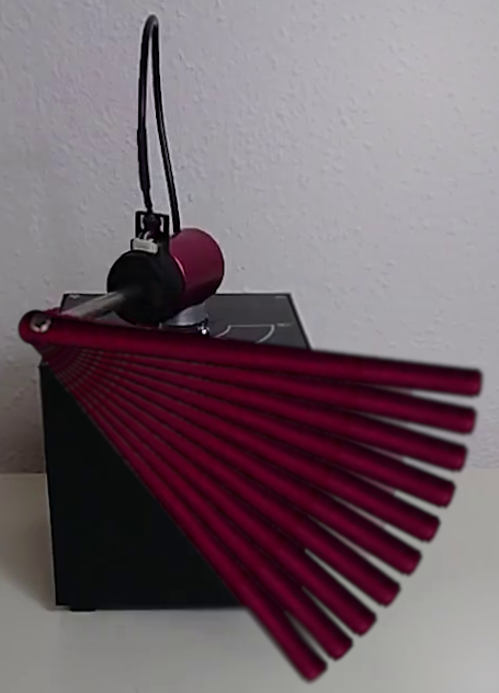
Figure 1: Evaluation platforms: (left) underactuated swing-up and balance task on the Quanser Furuta pendulum, (right) ball-in-a-cup task on the Barrett WAM robotic arm.

Moreover, we might face a situation where it is not affordable to improve the model. Alternatively, one can add variability to the generative model, e.g. by turning the physics simulator’s parameters into random variables. Learning from randomized simulations poses a harder problem for the learner due to the additional variability of the observed data. But the recent successes in the field of sim-to-real transfer argue for domain randomization being a promising method [3, 4].

State-of-the-art approaches commonly randomize the simulator according to a static handcrafted distribution [5, 6, 7, 8]. Even though static randomization is in many cases sufficient to cross the reality gap, it is desirable to automate the process as far as possible. Moreover, using a fixed distribution does not allow to update the prior knowledge or incorporate the uncertainty over domain parameters. Most importantly, closing the feedback loop over the real system will lead to policies with higher performance on the target domain since the feedback enables the optimization of the domain parameter distribution. However, approaches which adapt an distribution over simulators, yield to additional challenges. For example algorithms that intertwine system identification and policy optimization, e.g., [4, 9], introduce a circular dependency since both subroutines depend on the sensible outputs of the other. One possible failure case is a policy which does not excite the system well enough, resulting in bad updates the simulator’s parameters. The sim-to-real algorithm presented in this paper does not require any system identification.

Contributions

We advance the state-of-the-art by introducing Bayesian Domain Randomization (BayRn), a method which is able to close the reality gap by learning from randomized simulations and adapting the distribution over simulator parameters based solely on real-world returns. The use usage of Bayesian Optimization (BO) for sampling the next training environment (source domain) makes BayRn sample efficient w.r.t. real-world data. The proposed algorithm can be seen as a way to vastly automate the finding of a source domain distribution in sim-to-real settings, which is typically done by trial and error. We validate our approach by conducting a sim-to-sim as well as two sim-to-real experiments on an underactuated nonlinear swing-up task, and on a ball-in-a-cup task (Figure 1). The sim-to-sim setup examines the domain parameter adaptation mechanism of BayRn, and shows that the belief about the domain distribution parameters converges to a specified ground truth parameter set. In the sim-to-real experiments, we compare the performance of policies trained with BayRn against multiple baselines based on a total number of 700 real-world rollouts. Moreover, we demonstrate that BayRn is able to work with step-based as well as episodic Reinforcement Learning (RL) algorithms as policy optimization subroutines.

The remainder of this paper is organized as follows: first, we introduce the necessary fundamentals (Section II) for BayRn (Section III). Next, we evaluate the devised method experimentally (Section IV). Subsequently, we put BayRn into context with the related work (Section V). Finally, we conclude and mention possible future research directions (Section VI).

II Background and Notation

Optimizing control policies for Markov Decision Processes with unknown dynamics is generally a hard problem (Section II-A). It is specifically hard due to the simulation optimization bias [2], which occurs when transferring the polices learned in one domain to another. Adapting the source domain based on real-world data requires a method suited for expensive objective function evaluations. BO is a prominent choice for these kind of problems (Section II-B).

II-A Markov Decision Process

Consider a time-discrete dynamical system

$$\begin{gathered}\fs_{t+1}\sim\mathcal{P}_{\fxi}\left(\left.\fs_{t+1}\right|\fs_{t},\fa_{t},\fxi\right),\quad\fs_{0}\sim\mu_{0,\fxi}(\left.\fs_{0}\right|\fxi),\\ \fa_{t}\sim\pi\!\left(\left.\fa_{t}\right|\fs_{t};\ftheta\right),\quad\fxi\sim\nu\!\left(\fxi;\fphi\right),\end{gathered}$$ (1)

with the continuous state ${\fs_{t}\in\mathcal{S}_{\fxi}\subseteq\mathbb{R}^{{n_{s}}}}$, and continuous action ${\fa_{t}\in\mathcal{A}_{\fxi}\subseteq\mathbb{R}^{{n_{a}}}}$ at time step $t$. The environment, also called domain, is instantiated through its parameters ${\fxi\in\mathbb{R}^{{n_{\xi}}}}$ (e.g., masses, friction coefficients, or time delays), which are assumed to be random variables distributed according to the probability distribution ${\nu\colon\mathbb{R}^{{n_{\xi}}}\to\mathbb{R}^{+}}$ parametrized by $\fphi$. These parameters determine the transition probability density function ${\mathcal{P}_{\fxi}\colon\mathcal{S}_{\fxi}\times\mathcal{A}_{\fxi}\times\mathcal{S}_{\fxi}\to\mathbb{R}^{+}}$ that describes the system’s stochastic dynamics. The initial state $\fs_{0}$ is drawn from the start state distribution ${\mu_{0,\fxi}\colon\mathcal{S}_{\fxi}\to\mathbb{R}^{+}}$. Together with the reward function ${r\colon\mathcal{S}_{\fxi}\times\mathcal{A}_{\fxi}\to\mathbb{R}}$, and the temporal discount factor ${\gamma\in[0,1]}$, the system forms a MDP described by the set ${\mathcal{M}_{\fxi}=\{\mathcal{S}_{\fxi},\mathcal{A}_{\fxi},\mathcal{P}_{\fxi},\mu_{0,\fxi},r,\gamma\}}$. The goal of a Reinforcement Learning (RL) agent is to maximize the expected (discounted) return, a numeric scoring function which measures the policy’s performance. The expected discounted return of a stochastic domain-independent policy $\pi\!\left(\left.\fa_{t}\right|\fs_{t};\ftheta\right)$, characterized by its parameters $\ftheta\in\Theta\subseteq\mathbb{R}^{{n_{\theta}}}$, is defined as

$$J\!\left(\ftheta,\fxi,\fs_{0}\right)=\mathbb{E}_{\ftau\sim p(\ftau)}\!\Big{[}\sum_{t=0}^{T-1}\gamma^{t}r(\fs_{t},\fa_{t})\Big{|}\ftheta,\fxi,\fs_{0}\Big{]}.$$ (2)

While learning from experience, the agent adapts its policy parameters. The resulting state-action-reward tuples are collected in trajectories, a.k.a. rollouts, $\ftau=\{\fs_{t},\fa_{t},r_{t}\}_{t=0}^{T-1}$, with $r_{t}=r\!\left(\fs_{t},\fa_{t}\right)$. To keep the notation concise, we omit the dependency on $\fs_{0}$.

II-B Bayesian Optimization with Gaussian Processes

Bayesian Optimization (BO) is a sequential derivative-free global optimization strategy, which tries to optimize an unknown function $f\colon\mathcal{X}\rightarrow\mathbb{R}$ on a compact set $\mathcal{X}$ [10]. In order to do so, BO constructs a probabilistic model, typically a Gaussian Process (GP), for $f$. GPs are distributions over functions ${f\sim\mathcal{GP}\!\left(m,k\right)}$ defined by a prior mean $m\colon\mathcal{X}\rightarrow\mathbb{R}$ and positive definite covariance function $k\colon\mathcal{X}\times\mathcal{X}\rightarrow\mathbb{R}$ called kernel. This probabilistic model is used to make decisions about where to evaluate the unknown function next. A distinctive feature of BO is to use the complete history of noisy function evaluations ${\cal D}=\{\fx_{i},y_{i}\}_{i=0}^{n}$ with $\fx_{i}\in\mathcal{X}$ and $y_{i}\sim\mathcal{N}\left(y\big{|}f(\fx_{i}),\varepsilon\right)$ where $\varepsilon$ is the variance of the observation noise. The next evaluation candidate is then chosen by maximizing a so-called acquisition function $a\colon\mathcal{X}\rightarrow\mathbb{R}$, which typically balances exploration and exploitation. Prominent acquisition functions are Expected Improvement and Upper Confidence Bound. Through the use of priors over functions, BO has become a popular choice for sample-efficient optimization of black-box functions that are expensive to evaluate. Its sample efficiency plays well with the algorithm introduced in this paper where a GP models the relation between domain distribution’s parameters and the resulting policy’s return estimated from real-world rollouts, i.e. $\fx\equiv\fphi$ and $y\equiv\hat{J}^{\text{real}}\!\left(\ftheta^{\star}\right)$. For further information on BO and GPs, we refer the reader to [10] as well as [11].

III Bayesian Domain Randomization (BayRn)

The problem of source domain adaptation based on returns from the target domain can be expressed in a bilevel formulation

$$\fphi^{\star} =\operatorname*{arg\,max}_{\fphi\in\Phi}J^{\text{real}}\!\left(\ftheta^{\star}(\fphi)\right)\quad\text{with}$$ (3)

$$\ftheta^{\star}(\fphi) =\operatorname*{arg\,max}_{\ftheta\in\Theta}\mathbb{E}_{\fxi\sim\nu(\fxi;\fphi)}\!\left[J\!\left(\ftheta,\fxi\right)\right],$$ (4)

where we refer to (3) and (4) as the upper and lower level optimization problem respectively. Thus, the two equations state the goal of finding the set of domain distribution parameters $\fphi^{\star}$ that maximizes the return on the real-world target system $J^{\text{real}}\!\left(\ftheta^{\star}(\fphi)\right)$, when used to specify the distribution $\nu\!\left(\fxi;\fphi\right)$ during training in the source domain. The space of domain parameter distributions is represented by $\Phi$. In the following, we abbreviate $\ftheta^{\star}(\fphi)$ with $\ftheta^{\star}$.

input : domain parameter distribution $\nu\!\left(\fxi;\fphi\right)$, parameter space $\Phi=[\fphi_{\text{min}},\fphi_{\text{max}}]$, algorithm PolOpt, Gaussian Process $\mathcal{GP}$, acquisition function $a$, hyper-parameters $n_{\text{init}}$, $n_{\tau}$, $J^{\text{succ}}$

output : maximum a posteriori domain distribution parameter $\fphi^{\star}$ and policy $\pi\!\left(\ftheta^{\star}\right)$

1

$\triangleright$ Initialization phase

2 Initialize empty data set and $n_{\text{init}}$ policies randomly

3 ${\cal D}\leftarrow\{\}$ ; $\pi\!\left(\ftheta_{1:n_{\text{init}}}\right)\leftarrow\ftheta_{1:n_{\text{init}}}\sim\Theta$

4

5Sample $n_{\text{init}}$ source domain distribution parameter sets and train in randomized simulators

6

7$\fphi_{1:n_{\text{init}}}\leftarrow\fphi_{1:n_{\text{init}}}\sim\Phi$

8

9$\ftheta_{1:n_{\text{init}}}^{\star}\leftarrow\texttt{PolOpt}\!\left[\pi\!\left(\ftheta_{1:n_{\text{init}}}\right),\nu\!\left(\fxi;\fphi_{1:n_{\text{init}}}\right)\right]$

10

11Evaluate the $n_{\text{init}}$ policies on the target domain for $n_{\tau}$ rollouts and estimate the return

12$\hat{J}^{\text{real}}\!\left(\ftheta_{1:n_{\text{init}}}^{\star}\right)\leftarrow 1/n_{\tau}\sum_{j=1}^{n_{\tau}}$ $J_{j}^{\text{real}}\!\left(\ftheta_{1:n_{\text{init}}}^{\star}\right)$

13

14Augment the data set and update the GP’s posterior distribution

15

16${\cal D}\cup\{\fphi_{i},\hat{J}^{\text{real}}\!\left(\ftheta_{i}^{\star}\right)\}_{i=1}^{n_{\text{init}}}$ ; $\mathcal{GP}\!\left(m,k\right)\leftarrow\mathcal{GP}\big{(}m,k\big{|}{\cal D}\big{)}$

17

18do $\triangleright$ Sim-to-real loop

19       Optimize the GP’s acquisition function

20      

21      $\fphi^{\star}\leftarrow\operatorname*{arg\,max}_{\fphi\in\Phi}a\!\left(\fphi,{\cal D}\right)$

22      

23      Train a policy using the obtained domain distribution parameter set

24      $\ftheta^{\star}\leftarrow\texttt{PolOpt}\!\left[\pi\!\left(\ftheta\right),\nu\!\left(\fxi;\fphi^{\star}\right)\right]$

25      

26      Evaluate the policy on the target domain for $n_{\tau}$ rollouts and estimate the return

27      $\hat{J}^{\text{real}}\!\left(\ftheta^{\star}\right)\leftarrow 1/n_{\tau}\sum_{j=1}^{n_{\tau}}$ $J_{j}^{\text{real}}\!\left(\ftheta^{\star}\right)$

28      

29      Augment the data set and update the GP’s posterior distribution

30      

31      ${\cal D}\cup\{\fphi^{\star},\hat{J}^{\text{real}}\!\left(\ftheta^{\star}\right)\}$ ; $\mathcal{GP}\!\left(m,k\right)\leftarrow\mathcal{GP}\big{(}m,k\big{|}{\cal D}\big{)}$

32      

33while $\hat{J}^{\text{real}}\!\left(\ftheta^{\star}\right)<J^{\text{succ}}$ and $n_{\text{iter}}\leq n_{\text{iter,max}}$

Train the maximum a posteriori policy (repeat the Lines 1 and 1 once)

Algorithm 1 Bayesian Domain Randomization

At the core of BayRn, first a policy optimizer, e.g., an RL algorithm, is employed to solve the lower level problem (4) by finding a (locally) optimal policy $\pi\!\left(\ftheta^{\star}\right)$ for the current distribution of stochastic environments. This policy is evaluated on the real system for $n_{\tau}$ rollouts, providing an estimate of the return $\hat{J}^{\text{real}}\!\left(\ftheta^{\star}\right)$. Next, the upper level problem (3) is solved using BO, yielding a new domain parameter distribution which is used to randomize the simulator. In this process the relation between the domain distribution’s parameters $\fphi$ and the resulting policy’s return on the real system $\hat{J}^{\text{real}}\!\left(\ftheta^{\star}\right)$ is modeled by a GP. The GP’s mean and covariance is updated using all recorded inputs $\fphi$ and the corresponding observations $\hat{J}^{\text{real}}\!\left(\ftheta^{\star}\right)$. Finally, BayRn terminates when the estimated performance on the target system exceeds $J^{\text{succ}}$ which is the task-specific success threshold. Since the GP requires at least a few (about 5 to 10) samples to provide a meaningful posterior, BayRn has an initialization phase before the loop. In this phase, $n_{\text{init}}$ source domains are randomly sampled from $\Phi$, and subsequently for each of these domains a policy is trained. After evaluating the $n_{\text{init}}$ initial policies, the GP is fed with the inputs $\fphi_{1:n_{\text{init}}}$ and the corresponding observations $\hat{J}^{\text{real}}\!\left(\ftheta_{1:n_{\text{init}}}^{\star}\right)$. The complete BayRn procedure is summarized in Algorithm 1. In principle, there are no restrictions to the choice of algorithms for solving the two stages (3) and (4). For training the GP, we used the BO implementation from BoTorch [12] which expects normalized inputs and standardized outputs. Notably, we decided for the expected improvement acquisition function and a zero-mean GP prior with a Matérn 5/2 Kernel.

Connection to System Identification

Unlike related methods (Section V), BayRn does not include a term in the objective function that drives the system parameters to match the observed dynamics. Instead, the BO component in BayRn is free to adapt the domain distribution parameters $\fphi$ (e.g., mean or standard deviation of a body’s mass) while learning in simulation such that the resulting policies perform well in the target domain. This can be seen as an indirect system identification, since with increasing iteration count the BO process will converge to sampling from regions with high real-world return. There is a connection to control as inference approaches which interpret the cost as a log-likelihood function under an optimality criterion using a Boltzmann distribution construct [13, 14]. Regarding BayRn, the sequence of sampled domain distribution parameter sets strongly depends on the acquisition function and the complexity of the given problem. We argue that excluding system identification from the upper level objective (3) is sensible for the presented sim-to-real algorithm, since it learns from a randomized physics simulator, hence attenuates the benefit of a well-fitted model.

IV Experiments

We study Bayesian Domain Randomization (BayRn) on two different platforms: 1) an underactuated rotary inverted pendulum, also known as Furuta pendulum, with the task of swinging up the pendulum pole into an upright position, and 2) the tendon-driven 4-DoF robot arm WAM from Barrett, where the agent has to swing a ball into a cup mounted as the end-effector. First, we set up a simplified sim-to-sim experiment on the Furuta pendulum to check if the proposed algorithm’s belief about the domain distribution parameters converges to a specified set of ground truth values. Next, we evaluate BayRn as well as the baseline methods SimOpt [4], Uniform Domain Randomization (UDR), and Proximal Policy Optimization (PPO) [15] or Policy learning by Weighting Exploration with the Returns (PoWER) [16] in two sim-to-real experiments. Additional details on the system description can be found in Appendix A. Furthermore, an extensive list of the chosen hyper-parameters can be found in Appendix B. A video demonstrating the sim-to-real transfer of the policies learned with BayRn can be found at www.ias.informatik.tu-darmstadt.de/Team/FabioMuratore. Moreover, the source code of BayRn and the baselines is available at [17].

IV-A Experimental Setup

Figure 2: Platforms with annotated domain parameters

All rollouts on the Furuta pendulum ran for $6\text{\,}\mathrm{s}\text{/}$ at $100\text{\,}\mathrm{Hz}\text{/}$, collecting 600 time steps with a reward $r_{t}\in]0,1]$. We decided to use a Feedforward Neural Network (FNN) policy in combination with PPO as policy optimization (sub)routine (Table II(a)). Before each rollout, the platform was reset automatically. On the physical system, this procedure includes estimating the sensors’ offsets as well as running a controller which drives the device to its initial position with the rotary pole centered and the pendulum hanging down. In simulation, the reset function causes the simulator to sample a new set of domain parameters $\fxi$ (Figure 2). Due to the underactuated nature of the dynamics, the pendulum has to be swung back and forth to put energy into the system before being able to swing the pendulum up.

The Barrett WAM was operated at $500\text{\,}\mathrm{Hz}\text{/}$ with an episode length of $3.5\text{\,}\mathrm{s}\text{/}$, i.e., 1750 time steps. For the ball-in-cup task, we chose a RBF-policy commanding desired deltas to the current joint angles and angular velocities, which are passed to the robots feed-forward controller. Hence, the only input to the policy is the normalized time. At the beginning of each rollout, the robot is driven to an initial position. When evaluating on the physical platform, the ball needs to be manually stabilized in a resting position. Once the rollout has finished, the operator enters a return value (Appendix A).

Table I: Range of domain distribution parameter values $\fphi$ used during the experiments. All domain parameters were randomized such that they stayed physically plausible.

(a) swing-up and balance

Parameter	Range		Unit
pendulum pole mass mean	$\mathbb{E}\!\left[m_{p}\right]$	$\in[$0.0192$,$0.0288$]$	$\mathrm{k}\mathrm{g}$
pendulum pole mass var.	$\mathbb{V}\!\left[m_{p}\right]$	$\in[$5.7610-10$,$5.7610-6$]$	$\mathrm{k}\mathrm{g}\mathrm{{}^{2}}$
rotary pole mass mean	$\mathbb{E}\!\left[m_{r}\right]$	$\in[$0.076$,$0.114$]$	$\mathrm{k}\mathrm{g}$
rotary pole mass var.	$\mathbb{V}\!\left[m_{r}\right]$	$\in[$9.0310-9$,$9.0310-5$]$	$\mathrm{k}\mathrm{g}\mathrm{{}^{2}}$
pendulum pole length mean	$\mathbb{E}\!\left[l_{p}\right]$	$\in[$0.1032$,$0.1548$]$	$\mathrm{m}$
pendulum pole length var.	$\mathbb{V}\!\left[l_{p}\right]$	$\in[$1.6610-8$,$1.6610-4$]$	$\mathrm{m}\mathrm{{}^{2}}$
rotary pole length mean	$\mathbb{E}\!\left[l_{r}\right]$	$\in[$0.068$,$0.102$]$	$\mathrm{m}$
rotary pole length var.	$\mathbb{V}\!\left[l_{r}\right]$	$\in[$7.2310-9$,$7.2310-5$]$	$\mathrm{m}\mathrm{{}^{2}}$

(b) ball-in-a-cup

Parameter	Range		Unit
string length mean	$\mathbb{E}\!\left[l_{s}\right]$	$\in[$0.285$,$0.315$]$	$\mathrm{m}$
string length variance	$\mathbb{V}\!\left[l_{s}\right]$	$\in[$910-8$,$2.2510-4$]$	$\mathrm{m}\mathrm{{}^{2}}$
string damping mean	$\mathbb{E}\!\left[d_{s}\right]$	$\in[$0$,$210-4$]$	$\mathrm{N}\text{/}\mathrm{s}$
string damping variance	$\mathbb{V}\!\left[d_{s}\right]$	$\in[$3.3310-13$,$8.3310-10$]$	${\mathrm{N}}^{2}\text{/}{\mathrm{s}}^{2}$
ball mass mean	$\mathbb{E}\!\left[m_{b}\right]$	$\in[$0.0179$,$0.0242$]$	$\mathrm{kg}\text{/}$
ball mass variance	$\mathbb{V}\!\left[m_{b}\right]$	$\in[$4.4110-10$,$4.4110-6$]$	${\mathrm{kg}}^{2}\text{/}$
joint damping mean	$\mathbb{E}\!\left[d_{j}\right]$	$\in[$0.0$,$0.1$]$	$\mathrm{N}\text{/}\mathrm{s}$
joint damping variance	$\mathbb{V}\!\left[d_{j}\right]$	$\in[$3.3310-8$,$2.0810-4$]$	${\mathrm{N}}^{2}\text{/}{\mathrm{s}}^{2}$
joint stiction mean	$\mathbb{E}\!\left[\mu_{s}\right]$	$\in[$0$,$0.4$]$	$-$
joint stiction variance	$\mathbb{V}\!\left[\mu_{s}\right]$	$\in[$1.3310-6$,$3.3310-3$]$	$-$

In the sim-to-real experiments, we compare BayRn to SimOpt, UDR, and PPO or PoWER. For every algorithm, we train 20 polices and execute 5 evaluation rollouts per policy. PPO as well as PoWER are set up to learn from simulations where the domain parameters are given by the platforms’ data sheets or CAD models. These sets of domain parameters are called nominal. Hence, PPO and PoWER serve as a baseline representing step-based and episodic RL algorithms without domain randomization or any real-world data. UDR augments an RL algorithm, here PPO or PoWER, and can be seen as the straightforward way of randomizing a simulator, as done in [7]. Each domain parameter $\xi$ is assigned to an independent probability distribution, specified by its parameters $\fphi$, i.e. mean and variance, (Table I). Thus, we include UDR as a baseline method for static domain randomization. Note that UDR can, in contrast to BayRn and SimOpt, be easily parallelized which reduces the time to train a policy significantly. With SimOpt, Y. Chebotar et al. [4] presented a trajectory-based framework for closing the reality gap, and validated it on two state-of-the-art sim-to-real robotic manipulation tasks. SimOpt iteratively adapts the domain parameter distribution’s parameters by minimizing discrepancy between observations from the real-world system and the simulation. While BayRn formulates the upper level problem (3) solely based on the real-world returns, SimOpt minimizes a linear combination of the L1 and L2 norm between simulated and real trajectories. Moreover, SimOpt employs Relative Entropy Policy Search (REPS) [18] to update the simulator’s parameters, hence turning (3) into an RL problem. The necessity of real-world trajectories renders SimOpt unusable for the ball-in-a-cup task since the feed-forward policy is executed without recording any observations. Thus, there are no real-world trajectories with which to update the simulator. BayRn (Section III), SimOpt and UDR randomize the same domain parameters with identical nominal values. At the beginning of each sim-to-real experiment (Section IV-C), the domain distribution parameters $\fphi$ are sampled randomly from their ranges (Table I). The main difference is that BayRn and SimOpt adapt the domain distribution parameters, while UDR does not. We chose normal distributions for masses and lengths as well as uniform distributions for parameters related to friction and damping.

IV-B Sim-to-sim Results

(a) posterior mean

(b) posterior std.

Figure 3: Target domain returns 3(a) and the associated standard deviation 3(b) modeled by the GP learned with BayRn in a sim-to-sim setting (brighter is higher). The ground truth domain parameters as well as the maximum a posteriori domain distribution parameters found by BayRn are displayed as a red and orange star, respectively. The circles mark the sequence of domain parameter configurations (darker is later).

Before applying BayRn to a physical system, we examine the domain distribution parameter sampling process of the BO component in simulation. In order to provide a (qualitative) visualization, we chose to only randomize the means of the poles’ masses, i.e., $\fphi=[\mathbb{E}\!\left[m_{r}\right],\mathbb{E}\!\left[m_{p}\right]]^{\textsf{T}}$. Thus, for this sim-to-sim experiment the domain distribution parameters $\fphi$ are synonymous to the domain parameters $\fxi$. Apart from that, the hyper-parameters used for executing BayRn are identical to the ones used in the sim-to-real experiments (Appendix B).

(a) swing-up and balance

(b) ball-in-a-cup

Figure 4: Performance of the different algorithms across both sim-to-real tasks. For each algorithm 20 policies have been trained, varying the random seed, and evaluated 5 times to estimate the mean return per policy (700 rollouts in total). The median performance per algorithm is displayed by white circles, and the inner quartiles are represented by thick vertical bars. A dashed line in 4(a) marks an approximate threshold where the task is solved, i.e., the rotary pole is stabilized on top in the center. SimOpt was not applicable to our open-loop ball-in-a-cup task 4(b) because of its requirement for recorded observations.

As stated in Section III, BayRn was designed without an (explicit) system identification objective. However, we can see from Figure 3(a) that the maximizer of the GP’s mean function ${\fphi^{\star}=[0.0266,0.1084]^{\textsf{T}}}$ closely match the ground truth parameters $\fphi_{\text{GT}}=[0.0264,0.1045]^{\textsf{T}}$. Moreover, Figure 3(b) displays how the uncertainty about the target domain return is reduced in the vicinity of the sampled parameter configurations. There are two decisive factors for the domain distribution parameter sampling process: the acquisition function (Algorithm 1 Line 1), and the quality of the found policy (Algorithm 1 Line 1). Concerning the latter, a failed training run is indistinguishable to a successful one which fails to transfer to the target domain, since the GP only observes the estimated real-world return $\hat{J}^{\text{real}}\!\left(\ftheta^{\star}\right)$.

IV-C Sim-to-real Results

Figure 4 visualizes the results of the sim-to-real experiment described in Section IV-A. The discrepancy between the performance of PPO and PoWER and the other algorithms reveals that domain randomization was the decisive part for sim-to-real transferability. To verify that the PPO and PoWER learned meaningful policies, we checked them in the nominal simulation environments (not reported) and observed that they solve the tasks excellently. In Figure 4(a), we see that each median performance of BayRn, SimOpt, and UDR are above the success threshold. However, UDR has a significantly higher variance. SimOpt solves the swing-up and balance task in most cases. However, we noticed that the system identification subroutine can converge to extreme domain distribution parameters, rendering the next policy useless, which then yields a collection of poor trajectories for the next system identification, resulting in a downward spiral. BayRn on the other side relies on the policy optimizer’s ability to robustly solve the simulated environment (Section IV-B). This problem can be mediated by re-running the policy optimization in case a certain return threshold in simulation has not been exceeded. For the ball-in-a-cup task, Figure 4(b) shows an improvement of sim-to-real transfer for BayRn, especially since the tasks open-loop design amplifies domain mismatch. During the experiments, we noticed that UDR sometimes failed unexpectedly. We suspect the a high dependency on the initial state to be the reason for that.

Comparing the Furuta pendulum’s nominal domain parameters $\fphi_{\text{nom}}=[m_{p},m_{r},l_{p},l_{r}]^{\textsf{T}}=[0.024,0.095,0.129,0.085]^{\textsf{T}}$ to the means among BayRn’s final estimate $\fphi^{\star}_{\text{mean}}=[0.023,0.098,0.123,0.087]^{\textsf{T}}$, we see that the domain parameters’ means changed by less than $10\text{\,}\mathrm{\char 37\relax}\text{/}$ each. Complementary the variances among BayRn’s final estimate are $\fphi^{\star}_{\text{var}}=[$6.2910-8$,$5.6710-6$,$4.1010-5$,$1.1910-5$]^{\textsf{T}}$, indicating a higher uncertainty on the link lengths (relative to the means). Thus, the final domain parameters are well within the boundaries of the BO search space (Table I). In combination, these small differences result in significantly different system dynamics. We believe this to be the reason why the baselines without domain randomization completely failed to transfer.

V Related Work

We divide the related research on robot reinforcement learning from randomized simulations into approaches which use static (Section V-A) or adaptive (Section V-B) distributions for sampling the physics parameters. Bayesian Domain Randomization (BayRn) as introduced in Section III belongs to the second category.

V-A Domain Randomization with Static Distributions

Learning from a randomized simulator with fixed domain parameter distributions has bridged the reality gap in several cases [3, 6, 2]. Most prominently, the robotic in-hand manipulation reported in [3] showed that domain randomization in combination with careful model engineering and the usage of recurrent neural networks enables direct sim-to-real transfer on an unprecedented difficulty level. Similarly, Lowrey et al. [6] employed Natural Policy Gradient to learn a continuous controller for a positioning task, after carefully identifying the system’s parameters. Their results show that the policy learned from the identified model was able to perform the sim-to-real transfer, but the policies learned from an ensemble of models were more robust to modeling errors. Mordatch et al. [5] used finite model ensembles to run trajectory optimization on a small-scale humanoid robot. In contrast, Peng et al. [7] combined model-free RL with recurrent neural network policies trained on experience replay in order to push an object by controlling a robotic arm. The usage of risk-averse objective function has been explored on MuJoCo tasks in [19]. The authors also provide a Bayesian point of view.

Cully et al. [20] can be seen as an edge case of static and adaptive domain randomization, where a large set of policies is learned before execution on the physical robot and evaluated in simulation. Every policy is associated to one configuration of the so-called behavioral descriptors, which are related but not identical to domain parameters. In contrast to BayRn, there is no policy training after the initial phase. Instead of retraining or fine-tuning, the algorithm suggested in [20] reacts to performance drops, e.g. due to damage, by using BO to sequentially select a pretrained policy and measure its performance on the robot. The underlying GP models the mapping from behavior space to performance. This method demonstrated impressive damage recover abilities on a robotic locomotion and a reaching task. However, applying it to RL poses big challenges. Most notably, the number of policies to be learned in order to populate the map, scales exponentially with the dimension of the behavioral descriptors, potentially leading to a very large number of training runs.

Aside from to the previous methods, Muratore et al. [2] propose an approach to estimate the transferability of a policy learned from randomized physics simulations. Moreover, the authors propose a meta-algorithm which provides a probabilistic guarantee on the performance loss when transferring the policy between two domains form the same distribution.

Static domain randomization has also been successfully applied to computer vision problems. A few examples that are: (i) object detection [21], (ii) synthetic object generation for grasp planning [8], and (iii) autonomous drone flight [22].

V-B Domain Randomization with Adaptive Distributions

Ruiz et al. [23] proposed the meta-algorithm which is based on a bilevel optimization problem highly similar to the one of BayRn (3, 4). However, there are two major differences. First, BayRn uses Bayesian optimization on the acquired real-wold data to adapt the domain parameter distribution, whereas “learning to simulate” updates the domain parameter distribution using REINFORCE. Second, the approach in [23] has been evaluated in simulation on synthetic data, except for a semantic segmentation task. Thus, there was no dynamics-dependent interaction of the learned policy with the real world.

With SPRL, Klink et al. [24] derived a relative entropy RL algorithm that endows the agent to adapt the domain parameter distribution, typically from easy to hard instances. Hence, the overall training procedure can be interpreted as a curriculum learning problem. The authors were able to solve sim-to-sim goal reaching problems as well as a robotic sim-to-real ball-in-a-cup task, similar to the one in this paper. One decisive difference to BayRn is that the target domain parameter distribution has to be known beforehand.

The approach called Active Domain Randomization (ADR) [25] also formulates the adaption of the domain parameter distribution as an RL problem where different simulation instances are sampled and compared against a reference environment based on the resulting trajectories. This comparison is done by a discriminator which yields rewards proportional to the difficulty of distinguishing the simulated and real environments, hence providing an incentive to generate distinct domains. Using this reward signal, the domain parameters of the simulation instances are updated via Stein Variational Policy Gradient. Mehta et al. [25] evaluated their method in a sim-to-real experiment where a robotic arm had to reach a desired point. The strongest contrast between BayRn and ADR is they way in which new simulation environments are explored. While BayRn can rely on well-studied BO with an adjustable exploration-exploitation behavior, ADR can be fragile since it couples discriminator training and policy optimization, which results in a non-stationary process where distribution of the domains depends on the discriminator’s performance.

Paul et al. [26] introduce Fingerprint Policy Optimization which, like BayRn, employs BO to adapt the distribution of domain parameters such that using these for the subsequent training maximizes the policy’s return. At first glance the approaches look similar, but there is a major difference in how the upper level problem (3) is solved. Fingerprint Policy Optimization models the relation between the current domain parameters, the current policy and the return of the updated policy with a GP. This design decision requires to feed the policy parameters into the GP which is prohibitively expensive if done straightforwardly. Therefore, abstractions of the policy, so-called fingerprints, are created. These handcrafted features, e.g., the Gaussian approximation of the stationary state distribution, replace the policy to reduce the input dimension. The authors tested Fingerprint Policy Optimization on three sim-to-sim tasks. Contrarily, BayRn has been designed without the need to approximate the policy. Moreover, we validated the presented method in sim-to-real settings.

Yu et al. [9] intertwine policy optimization, system identification, and domain randomization. The proposed method first identifies bounds on the domain parameters which are later used for learning from the randomized simulator. The suggested policy is conditioned on a latent space projection of the domain parameters. After training in simulation, a second system identification step is executed to find the projected domain parameters which maximize the return on the physical robot. This step runs BO for a fixed number of iterations and is similar to solving the upper level problem in (3). The algorithm was evaluated on the bipedal walking robot Darwin OP2.

In Ramos et al. [27], likelihood-free inference in combination with mixture density random Fourier networks is employed to perform a fully Bayesian treatment of the simulator’s parameters. Analyzing the obtained posterior over domain parameters, Ramos et al. showed that BayesSim is, in a sim-to-sim setting, able to simultaneously infer different parameter configurations which can explain the observed trajectories. The key difference between BayRn and BayesSim is the objective for updating the domain parameters. While BayesSim maximizes the model’s posterior likelihood, BayRn updates the domain parameters such that the policy’s return on the physical system is maximized. The biggest advantage of BayRn over BayesSim is its ability to work with very sparse real-world data, i.e. only the scalar return values.

VI Conclusion

We have introduced Bayesian Domain Randomization (BayRn), a policy search algorithm tailored to crossing the reality gap. At its core, BayRn learns from a randomized simulator while using Bayesian optimization for adapting the source domain distribution during learning. In contrast to previous work, the presented algorithm constructs a probabilistic model of the connection between domain distribution parameters and the policy’s return after training with these parameters in simulation. Hence, BayRn only requires little interaction with the real-world system. We experimentally validated that the presented approach is able to solve two nonlinear robotic sim-to-real tasks. Comparing the results against baseline methods showed that adapting the domain parameter distribution lead to policies with higher median performance and less variance. In order to improve the scalability of the Bayesian optimization subroutine to higher numbers of domain distribution parameters, one could for example incorporate quantile Gaussian processes [28], which have shown to scales up to problems with 60-dimensional input.

Appendix A Modeling Details on the Platforms

The Furuta pendulum (Figure 1) is modeled as an underactuated nonlinear second-order dynamical system given by the solution of

$$\begin{bmatrix}J_{r}+m_{p}l_{r}^{2}+\frac{1}{4}m_{p}l_{p}^{2}(\mathrm{cos}\!\left(\alpha\right))^{2}&\frac{1}{2}m_{p}l_{p}l_{r}\mathrm{cos}\!\left(\alpha\right)\\ \frac{1}{2}m_{p}l_{p}l_{r}\mathrm{cos}\!\left(\alpha\right)&J_{p}+\frac{1}{4}m_{p}l_{p}^{2}\end{bmatrix}\begin{bmatrix}\ddot{\theta}\\ \ddot{\alpha}\end{bmatrix}=$$

$$\begin{bmatrix}\tau-\frac{1}{2}m_{p}l_{p}^{2}\mathrm{sin}\!\left(\alpha\right)\mathrm{cos}\!\left(\alpha\right)\dot{\theta}\dot{\alpha}-\frac{1}{2}m_{p}l_{p}l_{r}\mathrm{sin}\!\left(\alpha\right)\dot{\alpha}^{2}-d_{r}\dot{\theta}\\ -\frac{1}{4}m_{p}l_{p}^{2}\mathrm{sin}\!\left(\alpha\right)\mathrm{cos}\!\left(\alpha\right)\dot{\theta}^{2}-\frac{1}{2}m_{p}l_{p}g\mathrm{sin}\!\left(\alpha\right)-d_{p}\dot{\alpha}\\ \end{bmatrix},$$ (5)

with the rotary angle $\theta$ and the pendulum angle $\alpha$, which are defined to be zero when the rotary pole is centered and the pendulum pole is hanging down vertically. While the system’s state is defined as ${\fs=[\theta,\alpha,\dot{\theta},\dot{\alpha}]^{\textsf{T}}}$, the agent receives observations ${\fo=[\mathrm{sin}\!\left(\theta\right),\mathrm{cos}\!\left(\theta\right),\mathrm{sin}\!\left(\alpha\right),\mathrm{cos}\!\left(\alpha\right),\dot{\theta},\dot{\alpha}]^{\textsf{T}}}$. The horizontal pole is actuated by commanding a motor voltage (action) $a$ which regulates the servo motor’s torque ${\tau=k_{m}(a-k_{m}\dot{\theta})/R_{m}}$. One part of the domain parameters is sampled from distributions specified by in Table I(a), while the remaining domain parameters are fixed at their nominal values given in [17]. We formulate the reward function based on an exponentiated quadratic cost

$$\begin{gathered}r\!\left(\fs_{t},a_{t}\right)=\mathrm{exp}\left(-\left(\fe_{t}^{\textsf{T}}\fQ\fe_{t}+a_{t}Ra_{t}\right)\right)\quad\text{with}\\ \fe_{t}=\left(\begin{bmatrix}0&\pi&0&0\end{bmatrix}-\fs_{t}\right)\mod 2\pi.\end{gathered}$$ (6)

Thus, the reward is in range $]0,1]$ for every time step.

The 4-DoF Barrett WAM (Figure 1) is simulated using MuJoCo, wrapped by mujoco-py [29]. The ball is attached to a string, which is mounted to the center of the cup’s bottom plate. We model the string as a concatenation of 30 rigid bodies with two rotational joints per link (no torsion). This specific ball-in-a-cup instance can be considered difficult, since the cups’s diameter is only about twice as large as the ball’s, and the string is rather short with a length of $30\text{\,}\mathrm{cm}\text{/}$. Similar to the Furuta pendulum, one part of the domain parameters is sampled from distributions specified by in Table I(b), while the remaining domain parameters are fixed at their nominal values given in [17]. Since the feed-forward policy is executed without recording any observations, we define a discrete ternary reward function

$$r\!\left(\fs_{T},\fa_{T}\right)=\begin{cases}1&\text{if the ball is in the cup,}\\ 0.5&\text{if the ball hit the cup's upper rim,}\\ 0&\text{else}\end{cases}$$ (7)

where the final reward given by the operator after the rollout ($r\!\left(\fs_{t},\fa_{t}\right)=0$ for $t<T$) when running on the real system. We found the separation in three cases to be helpful during learning and easily distinguishable from the others. While training in simulation, successful trials are identified by detecting a collision between the ball and a virtual cylinder inside the cup. Moreover, we have access to the full state, hence augment the reward function with a cost term that punishes deviations from the initial end-effector position.

Appendix B Parameter Values for the Experiments

Table II lists the hyper-parameters for all training runs during the experiments in Section IV. The reported values have been tuned but not fully optimized.

Table II: Hyper-parameter values for training the policies in Section IV. The domain distribution parameters $\fphi$ are listed in Table I.

(a) swing-up and balance

Hyper-parameter	Value
common
PolOpt	PPO
policy / critic architecture	FNN $64$-$64$ with tan-h
optimizer	Adam
learning rate policy	$5.9710-4$
learning rate critic	$3.4410-4$
PPO clipping ratio $\epsilon$	$0.1$
iterations $n_{\text{iter}}$	$300$
step size $\Delta t$	$0.01\text{\,}\mathrm{s}\text{/}$
max. steps per episode $T$	$600$
min. steps per iteration	$20$$T$
temporal discount $\gamma$	$0.9885$
adv. est. trade-off factor $\lambda$	$0.965$
success threshold $J^{\text{succ}}$	$375$
$\fQ$	$\textrm{diag}($210-1$,$1.0$,$210-2$,$510-3$)$
$R$	$310-3$
real-world rollouts $n_{\tau}$	$5$
UDR specific
min. steps per iteration	$30$$T$
SimOpt specific
max. iterations $n_{\text{iter}}$	$15$
DistrOpt population size	$500$
DistrOpt KL bound $\epsilon$	$1.0$
DistrOpt learning rate	$510-4$
BayRn specific
max. iterations $n_{\text{iter,max}}$	$15$
initial solutions $n_{\text{init}}$	$5$

(b) ball-in-a-cup

Hyper-parameter	Value
common
PolOpt	PoWER
policy architecture	RBF with 16 basis functions
iterations $n_{\text{iter}}$	$20$
population size $n_{\text{pop}}$	$100$
num. importance samples $n_{\text{is}}$	$10$
init. exploration std $\sigma_{\text{init}}$	$\pi/12$
min. rollouts per iteration	$20$
max. steps per episode $T$	$1750$
step size $\Delta t$	$0.002\text{\,}\mathrm{s}\text{/}$
temporal discount $\gamma$	$1$
real-world rollouts $n_{\tau}$	$5$
UDR specific
min. steps per iteration	$30$$T$
BayRn specific
max. iterations $n_{\text{iter}}$	$15$
initial solutions $n_{\text{init}}$	$5$

References

- Hobbs and Hepenstal [1989] B. F. Hobbs and A. Hepenstal, “Is optimization optimistically biased?” Water Resources Research, vol. 25, no. 2, pp. 152–160, 1989.
- Muratore et al. [2019] F. Muratore, M. Gienger, and J. Peters, “Assessing transferability from simulation to reality for reinforcement learning,” PAMI, vol. PP, pp. 1–1, 11 2019.
- OpenAI et al. [2018] OpenAI et al., “Learning dexterous in-hand manipulation,” ArXiv eprints, vol. 1808.00177, 2018.
- Y. Chebotar et al. [2019] Y. Chebotar et al., “Closing the sim-to-real loop: Adapting simulation randomization with real world experience,” in ICRA, Montreal, QC, Canada, May 20-24, 2019, pp. 8973–8979.
- Mordatch et al. [2015] I. Mordatch, K. Lowrey, and E. Todorov, “Ensemble-cio: Full-body dynamic motion planning that transfers to physical humanoids,” in IROS, Hamburg, Germany, September 28 - October 2, 2015, pp. 5307–5314.
- Lowrey et al. [2018] K. Lowrey, S. Kolev, J. Dao, A. Rajeswaran, and E. Todorov, “Reinforcement learning for non-prehensile manipulation: Transfer from simulation to physical system,” in SIMPAR 2018, Brisbane, Australia, May 16-19, 2018, pp. 35–42.
- Peng et al. [2018] X. B. Peng, M. Andrychowicz, W. Zaremba, and P. Abbeel, “Sim-to-real transfer of robotic control with dynamics randomization,” in ICRA, Brisbane, Australia, May 21-25, 2018, pp. 1–8.
- J. Tobin et al. [2018] J. Tobin et al., “Domain randomization and generative models for robotic grasping,” in IROS, Madrid, Spain, October 1-5, 2018.
- Yu et al. [2019] W. Yu, V. C. V. Kumar, G. Turk, and C. K. Liu, “Sim-to-real transfer for biped locomotion,” in IROS, Macau, SAR, China, November 3-8. IEEE, 2019, pp. 3503–3510.
- Snoek et al. [2012] J. Snoek, H. Larochelle, and R. P. Adams, “Practical bayesian optimization of machine learning algorithms,” in NIPS, Lake Tahoe, Nevada, United States, December 3-6, 2012, pp. 2960–2968.
- Rasmussen and Williams [2006] C. E. Rasmussen and C. K. I. Williams, Gaussian processes for machine learning, ser. Adaptive computation and machine learning. MIT Press, 2006.
- Balandat et al. [2019] M. Balandat, B. Karrer, D. R. Jiang, S. Daulton, B. Letham, A. G. Wilson, and E. Bakshy, “BoTorch: Programmable bayesian optimization in pytorch,” ArXiv e-prints, 2019.
- Toussaint [2009] M. Toussaint, “Robot trajectory optimization using approximate inference,” in ICML Montreal, Quebec, Canada, June 14-18, vol. 382, 2009, pp. 1049–1056.
- Rawlik et al. [2013] K. Rawlik, M. Toussaint, and S. Vijayakumar, “On stochastic optimal control and reinforcement learning by approximate inference,” in IJCAI, Beijing, China, August 3-9, 2013, pp. 3052–3056.
- Schulman et al. [2017] J. Schulman, F. Wolski, P. Dhariwal, A. Radford, and O. Klimov, “Proximal policy optimization algorithms,” ArXiv e-prints, 2017.
- Kober and Peters [2011] J. Kober and J. Peters, “Policy search for motor primitives in robotics,” Machine Learning, vol. 84, no. 1-2, pp. 171–203, 2011.
- Muratore [2020] F. Muratore, “SimuRLacra - a framework for reinforcement learning from randomized simulations,” https://github.com/famura/SimuRLacra, 2020.
- Peters et al. [2010] J. Peters, K. Mülling, and Y. Altun, “Relative entropy policy search,” in AAAI, Atlanta, Georgia, USA, July 11-15, 2010.
- Rajeswaran et al. [2017] A. Rajeswaran, S. Ghotra, B. Ravindran, and S. Levine, “Epopt: Learning robust neural network policies using model ensembles,” in ICLR, Toulon, France, April 24-26, 2017.
- Cully et al. [2015] A. Cully, J. Clune, D. Tarapore, and J.-B. Mouret, “Robots that can adapt like animals,” Nature, vol. 521, no. 7553, pp. 503–507, 2015.
- J. Tobin et al. [2017] J. Tobin et al., “Domain randomization for transferring deep neural networks from simulation to the real world,” in IROS, Vancouver, BC, Canada, September 24-28, 2017, pp. 23–30.
- Sadeghi and Levine [2017] F. Sadeghi and S. Levine, “CAD2RL: real single-image flight without a single real image,” in RSS, Cambridge, Massachusetts, USA, July 12-16, 2017.
- Ruiz et al. [2018] N. Ruiz, S. Schulter, and M. Chandraker, “Learning to simulate,” ArXiv e-prints, vol. 1810.02513, 2018.
- Klink et al. [2019] P. Klink, H. Abdulsamad, B. Belousov, and J. Peters, “Self-paced contextual reinforcement learning,” ArXiv e-prints, vol. 1910.02826, 2019.
- Mehta et al. [2019] B. Mehta, M. Diaz, F. Golemo, C. J. Pal, and L. Paull, “Active domain randomization,” in CoRL, Osaka, Japan, October 30 - November 1, vol. 100. PMLR, 2019, pp. 1162–1176.
- Paul et al. [2018] S. Paul, M. A. Osborne, and S. Whiteson, “Fingerprint policy optimisation for robust reinforcement learning,” ArXiv e-prints, vol. 1805.10662, 2018.
- Ramos et al. [2019] F. Ramos, R. Possas, and D. Fox, “Bayessim: Adaptive domain randomization via probabilistic inference for robotics simulators,” in RSS, University of Freiburg, Freiburg im Breisgau, Germany, June 22-26, 2019.
- Moriconi et al. [2020] R. Moriconi, K. S. S. Kumar, and M. P. Deisenroth, “High-dimensional bayesian optimization with projections using quantile gaussian processes,” Optim. Lett., vol. 14, no. 1, pp. 51–64, 2020.
- [29] “mujoco-py,” Online. [Online]. Available: https://github.com/openai/mujoco-py