Global fixed points of mapping class group actions and a theorem of Markovic

Abstract.

We give a short and elementary proof of the non-realizability of the mapping class group via homeomorphisms. This was originally established by Markovic, resolving a conjecture of Thurston. With the tools established in this paper, we also obtain some rigidity results for actions of the mapping class group on Euclidean spaces.

1. introduction

In this paper, we discuss a new strategy to study Nielsen’s realization problem. We will use this to give a new and very simple proof of the main result of [7].

Let $\Sigma_{g}$ be the surface of genus $g$ and $\operatorname{Homeo}_{+}(\Sigma_{g})$ the group of orientation-preserving homeomorphisms of $\Sigma_{g}$. Denote by $\operatorname{Mod}(\Sigma_{g}):=\pi_{0}(\operatorname{Homeo}_{+}(\Sigma_{g}))$ the mapping class group of $\Sigma_{g}$. The Nielsen realization problem asks whether the natural projection

$$p_{g}:\operatorname{Homeo}_{+}(\Sigma_{g})\to\operatorname{Mod}(\Sigma_{g})$$

has a group-theoretic section (this particular formulation is attributed to Thurston; c.f. [5, Problem 2.6]). The realization problem can also be posed for other regularities and for arbitrary subgroups of $\operatorname{Mod}(\Sigma_{g})$, and there is a rich literature on the many variants that arise. We refer the reader for the survey paper [8] for further discussion.

In [7], Markovic shows that $p_{g}$ has no section for $g>5$. The proof is very involved and uses many dynamical tools. The main result of this note gives an elementary proof of his result in the optimal range $g\geq 2$.

Theorem 1.1.

For $g\geq 2$, the projection $p_{g}$ has no sections.

We obtain this as a consequence of a rigidity theorem for actions of a closely related group. Let $\Sigma_{g,1}$ be the surface of genus $g$ with one marked point and let $\operatorname{Homeo}_{+}(\Sigma_{g,1})$ denote the group of orientation-preserving homeomorphisms of $\Sigma_{g,1}$ that fix the marked point. Define $\operatorname{Mod}(\Sigma_{g,1}):=\pi_{0}(\operatorname{Homeo}_{+}(\Sigma_{g,1}))$ to be the “pointed mapping class group” of $\Sigma_{g,1}$.

Theorem 1.2.

For $g\geq 2$, any nontrivial action of $\operatorname{Mod}(\Sigma_{g,1})$ on $\operatorname{\mathbb{R}}^{2}$ by homeomorphisms has a global fixed point.

We now explain how Theorem 1.2 implies Theorem 1.1.

Proof.

Let $\operatorname{Homeo}_{+}(\operatorname{\mathbb{D}}^{2})^{\pi_{1}(S_{g})}$ denote the group of $\pi_{1}(\Sigma_{g})$-equivariant orientation-preserving homeomorphisms of the universal cover $\operatorname{\mathbb{D}}^{2}$ of $\Sigma_{g}$. This is compatible with the Birman exact sequence for the mapping class group, realizing $\operatorname{Homeo}_{+}(\operatorname{\mathbb{D}}^{2})^{\pi_{1}(S_{g})}$ as the pullback of $\operatorname{Homeo}_{+}(\Sigma_{g})$ and $\operatorname{Mod}(\Sigma_{g,1})$ along $\operatorname{Mod}(\Sigma_{g})$:

By the universal property of pullbacks, a section of $p_{g}$ gives rise to a section of $p_{g}^{\prime}$; any such section $p_{g}^{\prime}$ must realize $\pi_{1}(\Sigma_{g})$ as the group of deck transformations of $\Sigma_{g}$.

By Theorem 1.2, the action of $\operatorname{Mod}(\Sigma_{g,1})$ on $\operatorname{\mathbb{D}}^{2}\cong\mathbb{R}^{2}$ via a section of $p_{g}^{\prime}$ has a global fixed point, which contradicts the fact that deck transformations act freely. ∎

The same set of ideas also leads to a rigidity theorem for mapping class group actions on $\mathbb{R}^{3}$ in the regime $g\geq 4$.

Theorem 1.3.

For $g\geq 4$, any nontrivial continuous action of $\operatorname{Mod}(\Sigma_{g,1})$ on $\operatorname{\mathbb{R}}^{3}$ has a globally-invariant line.

Corollary 1.4.

For $g\geq 4$, there is no action of $\operatorname{Mod}(\Sigma_{g,1})$ on $\operatorname{\mathbb{R}}^{2}$ and $\operatorname{\mathbb{R}}^{3}$ by $C^{1}$ diffeomorphisms.

All of the above results are an easy consequence of the following structural result for $\operatorname{Mod}(\Sigma_{g,1})$. For an element $f$ of a group $G$, we write $C(f)$ to denote the centralizer of $f$ in $G$. Also recall that a homeomorphism $\iota$ is said to be hyperelliptic if $\iota$ has order $2$ and has exactly $2g+2$ fixed points. A mapping class is said to be hyperelliptic if it admits a hyperelliptic representative.

Theorem 1.5.

For $g\geq 2$, there exists an order $6$ element $\alpha_{g}\in\operatorname{Mod}(\Sigma_{g,1})$ such that

$$\Gamma:=\langle C(\alpha_{g}^{2}),C(\alpha_{g}^{3})\rangle$$

is the full mapping class group:

$$\Gamma=\operatorname{Mod}(\Sigma_{g,1}).$$

If $g\neq 3$, then $\alpha_{g}$ can be constructed so that $\alpha_{g}^{3}$ is not hyperelliptic.

Problem 1.6.

If $\beta\in\operatorname{Mod}(\Sigma_{g,1})$ is a torsion element of order divisible by two distinct primes $p,q$, then there is no a priori obstruction for $\operatorname{Mod}(\Sigma_{g,1})$ to be generated by $C(\beta^{p})$ and $C(\beta^{q})$. Does the conclusion of Theorem 1.5 hold for any torsion element $\beta$ with order not a prime power?

We now explain how Theorem 1.5 implies Theorem 1.2. In Section 5, we show how Theorem 1.5 also implies Theorem 1.3 and Corollary 1.4 via a short argument in local Smith theory.

Proof.

Since $\operatorname{Mod}(\Sigma_{g,1})$ is perfect, it has no nontrivial maps to $\mathbb{Z}/2$. Thus any action on $\mathbb{R}^{n}$ is orientation-preserving. Let $\alpha_{g}$ be the symmetry of Theorem 1.5. Any continuous action of the finite-order element $\alpha_{g}$ on $\mathbb{R}^{2}$ has a unique fixed point $O$ (see [2] and [10]). Since this fixed point is unique, both $C(\alpha_{g}^{2})$ and $C(\alpha_{g}^{3})$ fix $O$. By Theorem 1.5, $\operatorname{Mod}(\Sigma_{g,1})$ fixes $O$, showing Theorem 1.2. ∎

In the remainder of this note we construct the symmetry $\alpha_{g}$ and establish the properties claimed in Theorem 1.5. In Section 2 we describe our models of $\Sigma_{g,1}$ equipped with the symmetry $\alpha_{g}$; we use a different model for each residue class $g\pmod{3}$. In Section 3, we discuss a special class of curves and subsurfaces on these model subsurfaces that feature in the proof of Theorem 1.5. We carry out the proof of Theorem 1.5 in Section 4. Finally, we deduce Theorem 1.3 and Corollary 1.4 from Theorem 1.5 in Section 5.

Acknowledgements. The authors would like to thank Vlad Markovic for helpful discussions.

2. Models

The aim of this section is to construct, for each $g\geq 2$, a certain symmetry $\alpha_{g}\in\operatorname{Mod}(\Sigma_{g,1})$ of order $6$. The proof of Theorem 1.5 in Section 4 requires the existence of certain configurations of symmetric curves which are easy to find only for certain conjugacy classes of order-$6$ elements of $\operatorname{Mod}(\Sigma_{g,1})$; this is why we must take care in constructing our symmetries. The Riemann–Hurwitz formula (c.f. Lemma 2.1) implies that different constructions are necessary for each residue class of $g\pmod{3}$. In order to give as uniform a presentation as possible, we represent each “model surface” as a disk with pairs of boundary segments identified; the rules for edge identification are specified by the data of a “monodromy tuple” to be presented below (see the table in (2)).

For $g\neq 3$, the symmetries we use (and the corresponding symmetric surfaces) are depicted in Figure 1. The case $g=3$ requires special consideration; the model we use is shown in Figure 6. The discussion leading up to Figure 1 is not absolutely required to make sense of Figure 1, but is included so as to help orient the reader.

2.1. Branched covers

The symmetries we construct are realized as deck transformations of $\mathbb{Z}/6\mathbb{Z}$-branched covers of $S^{2}$. Here we recall the basic topological theory of branched coverings. Fix a group $G$ and surfaces $X$ and $Y$; we also fix the branch locus $B\subset Y$, a finite set of points. A branched covering $f:X\to Y$ with covering group $G$ branched over $B$ is then specified by a surjective homomorphism $\rho:\pi_{1}(Y\setminus B)\to G$. The preimage $f^{-1}(B)$ is the ramification set and the elements are ramification points. A point $x\in X$ is ramified if and only if $\operatorname{Stab}_{G}(x)$ is nontrivial; in this case, the order of $x$ is defined to be the order of $\operatorname{Stab}_{G}(x)$.

When $Y=S^{2}$ is a sphere, this can be further combinatorialized. Enumerate $B=\{b_{1},\dots,b_{n}\}$, and choose an identification

$$\pi_{1}(S^{2}\setminus B)\cong\langle a_{1},\dots,a_{n}\mid a_{1}\dots a_{n}=1\rangle;$$

here each $a_{i}$ runs from a basepoint $p\in S^{2}$ to a small loop around $b_{i}$. The local monodromy at $b_{i}$ is the corresponding element $\rho(a_{i})\in G$. Without loss of generality we can assume that each $\rho(a_{i})\neq 1$. The monodromy vector is the associated tuple $(\rho(a_{1}),\dots,\rho(a_{n}))\in G^{n}$. Note that necessarily $\rho(a_{1})\dots\rho(a_{n})=1$, and conversely, any such $n$-tuple gives rise to a branched $G$-cover.

For the purposes of this paper we will only be concerned with the case $G=\mathbb{Z}/6\mathbb{Z}$, and we adopt some further notation special to this situation. With the branch set $B\subset S^{2}$ fixed, we observe that each branch point $b_{i}$ has corresponding order $|\rho(a_{i})|\in\{2,3,6\}$. Define $p$ (resp. $q$ or $r$) as the number of points of order $6$ (resp. $3$ or $2$). We define the branching vector as the tuple $(p,q,r)$. The lemma below records the Riemann–Hurwitz formula specialized to this setting.

Lemma 2.1.

Let $f:\Sigma_{g}\to S^{2}$ be a $\mathbb{Z}/6\mathbb{Z}$-branched covering with branching vector $(p,q,r)$. Then

$$5p+4q+3r=10+2g.$$

Monodromy tuples. As a final specialization, we can shorten our notation for the monodromy vector at the cost of possibly re-ordering the elements of $B$. Suppose that $1\in\mathbb{Z}/6\mathbb{Z}$ appears $a$ times, $2\in\mathbb{Z}/6\mathbb{Z}$ appears $b$ times, etc. Up to a re-ordering of $B$, this data can be captured in the monodromy tuple. To make the computation of the associated $p,q,r$ more transparent, we order the elements of $\mathbb{Z}/6\mathbb{Z}$ according to their group-theoretic order. Thus a monodromy tuple is a symbol of the following form:

$$1^{a}\ 5^{p-a}\ 2^{b}\ 4^{q-b}\ 3^{r}.$$ (1)

2.2. The model surfaces

The elements $\alpha_{g}$ of Theorem 1.5 will be constructed as deck transformations associated to regular $\mathbb{Z}/6\mathbb{Z}$ covers of $S^{2}$ as in the previous subsection. We will require different constructions for the three different residue classes $g\pmod{3}$ and a special construction for $g=3$. Below, we specify $k\geq 0$. As the final column shows, for $g\neq 3$, the power $\alpha_{g}^{3}$ has strictly fewer than $2g+2$ fixed points and hence is not hyperelliptic.

$$\begin{array}[]{|c|c|c|c|}\hline\cr g&(p,q,r)&\text{tuple}&\text{number of branched points of $\alpha_{g}^{3}$}\\ \hline\cr 2+3k&(2,1,2k)&1^{2}\ 4\ 3^{2k}&2k\times 3+2<2g+2\\ 3&(2,0,2)&1\ 5\ 3^{2}&8=2g+2\\ 3+3(k+1)&(3,1,2k+1)&1^{2}\ 5\ 2\ 3^{2k+1}&(2k+1)\times 3+3<2g+2\\ 4+3k&(3,0,2k+1)&1^{3}\ 3^{2k+1}&(2k+1)\times 3+3<2g+2\\ \hline\cr\end{array}$$ (2)

$g\equiv 2\pmod{3}$ at 100 250 $1$ [bl] at 158.73 388.31 $2$ [br] at 56.69 399.65 $3$ [br] at 0.00 320.28 $4$ [tr] at 36.85 229.58 $5$ [bl] at 198.41 315.28 $6$ [tl] at 195.57 299.78 $1$ [br] at 36.85 388.31 $2$ [tr] at 0.00 300.78 $3$ [tr] at 59.52 215.41 $4$ [tl] at 158.73 226.75 $5$ [tl] at 136.05 215.41 $6$ [bl] at 138.88 399.65 $x$ [tr] at 141.72 385.48 $g\equiv 0\pmod{3}$ at 220 40 $1$ [bl] at 277.77 175.73 $2$ [br] at 178.57 189.90 $3$ [br] at 119.04 110.54 $4$ [tr] at 155.89 17.01 $5$ [tl] at 260.76 5.67 $6$ [tl] at 317.45 85.03 $1$ [br] at 155.89 178.57 $2$ [tr] at 119.04 85.03 $3$ [tr] at 178.57 5.67 $4$ [tl] at 277.77 17.01 $5$ [bl] at 317.45 110.54 $6$ [bl] at 257.93 189.90 $x$ [tr] at 263.60 175.73 $g\equiv 1\pmod{3}$ at 340 250 $1$ [bl] at 397.77 385.73 $2$ [br] at 298.57 394.90 $3$ [br] at 239.04 315.54 $4$ [tr] at 275.89 232.01 $5$ [tl] at 380.76 219.67 $6$ [tl] at 437.45 297.03 $1$ [br] at 275.89 383.57 $2$ [tr] at 239.04 297.03 $3$ [tr] at 298.57 217.67 $4$ [tl] at 397.77 229.01 $5$ [bl] at 437.45 315.54 $6$ [bl] at 377.93 394.90 $x$ [tr] at 383.60 390.73

$1^{\prime}$ [b] at 121.88 402.48 $2^{\prime}$ [tl] at 167.23 235.25 $2^{\prime}$ [tr] at 5.67 269.27 $4^{\prime}$ [br] at 28.34 379.81 $5^{\prime}$ [bl] at 195.57 331.62 $5^{\prime}$ [tr] at 85.03 209.74 $1^{\prime}$ [tl] at 175.73 246.59 $3^{\prime}$ [tr] at 0 283.44 $3^{\prime}$ [b] at 110.54 405.15 $4^{\prime}$ [bl] at 189.90 345.79 $6^{\prime}$ [tr] at 70.86 212.58 $6^{\prime}$ [br] at 19.84 368.47 $1^{\prime}$ [b] at 240.92 195.57 $6^{\prime}$ [br] at 144.55 167.23 $5^{\prime}$ [tr] at 121.88 70.86 $4^{\prime}$ [tl] at 192.74 2.83 $3^{\prime}$ [tl] at 289.11 28.34 $2^{\prime}$ [bl] at 314.62 121.88 $5^{\prime}$ [br] at 136.05 153.06 $4^{\prime}$ [tr] at 127.55 56.85 $3^{\prime}$ [t] at 209.74 0.00 $2^{\prime}$ [tl] at 297.61 42.52 $1^{\prime}$ [bl] at 308.95 141.72 $6^{\prime}$ [b] at 226.75 195.57 $1^{\prime\prime}$ [b] at 215.92 195.57 $3^{\prime\prime}$ [b] at 201.75 195.57 $4^{\prime\prime}$ [br] at 134.55 140.23 $6^{\prime\prime}$ [br] at 131.05 130.06 $5^{\prime\prime}$ [tl] at 216.74 2.83 $2^{\prime\prime}$ [tl] at 305.11 55.34 $6^{\prime\prime}$ [bl] at 299.62 146.88 $1^{\prime\prime}$ [tr] at 142.55 38.85 $4^{\prime\prime}$ [t] at 234.74 5.00 $3^{\prime\prime}$ [tl] at 307.61 66.52 $5^{\prime\prime}$ [bl] at 291.95 158.72 $2^{\prime\prime}$ [tr] at 135.88 47.86

$1^{\prime}$ [b] at 360.92 405.57 $2^{\prime}$ [br] at 264.55 377.23 $3^{\prime}$ [tr] at 241.88 280.86 $4^{\prime}$ [tl] at 307.74 212.83 $5^{\prime}$ [tl] at 409.11 238.34 $6^{\prime}$ [bl] at 434.62 331.88 $1^{\prime}$ [br] at 256.05 363.06 $2^{\prime}$ [tr] at 250.55 266.85 $3^{\prime}$ [t] at 329.74 210.00 $4^{\prime}$ [tl] at 417.61 252.52 $5^{\prime}$ [bl] at 428.95 351.72 $6^{\prime}$ [b] at 346.75 405.57

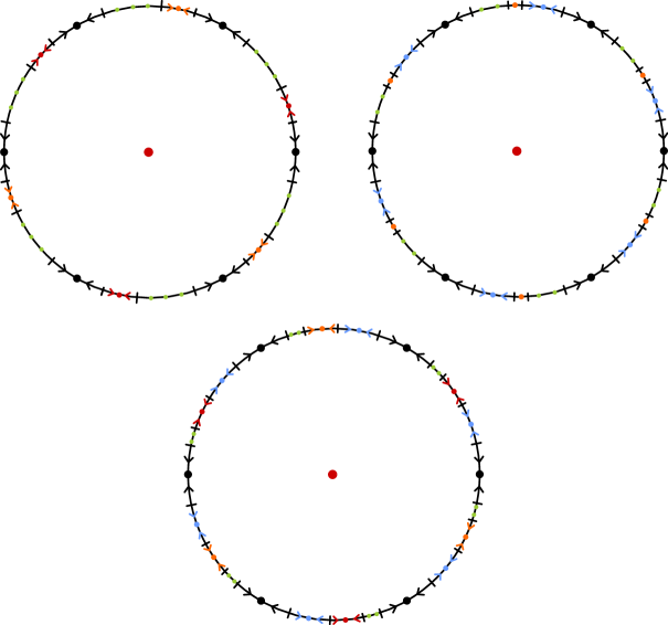
Figure 1. The model surfaces for $g\neq 3$: each is constructed by taking the disk $D$ and identifying the specified edge segments of $\partial D$. In each case, $\alpha_{g}$ is represented as a rotation by $2\pi/6$ about the center of the disk. We adopt the convention that we do not specify labeling data for points where the local monodromy is of order $2$; in each such case, the point and its corresponding segment of $\partial D$ is identified with the segment directly opposite on $D$. This is true in particular for the $k\geq 0$ points in green in each sector, which correspond to the portion of the monodromy tuple of the form $3^{2k}$.

To represent $\Sigma_{g,1}$ with its symmetry $\alpha_{g}$ as in (2), we adopt the models shown in Figure 1, where $\Sigma_{g,1}$ is given as a (marked) disk $D$ with edge identifications. See Figure 1 and its caption for a detailed discussion. We emphasize that the marked point $x\in\Sigma_{g,1}$ is not the fixed point at the center, but rather one of the fixed points on $\partial D$ (labeled, and drawn with a heavy dot). The model surface for $g=3$ is given in Figure 6.

For the purpose of later discussion, we observe here a simple property of this construction.

Definition 2.2 (Edge type).

Let $e$ be an edge of $\partial D$. By construction, exactly one endpoint of $e$ is a ramification point. We say that $e$ is type $p$ (resp. type $q$, type $r$) if this ramification point has order $6$ (resp. $3$, $2$).

3. Chords and convexity

In this section we develop some language for discussing a special class of curves and subsurfaces on the model surfaces. This is based around an ad-hoc identification of the disk $D$ with the hyperbolic disk $\mathbb{D}^{2}$. We will find it convenient to consider representatives for curves on $\Sigma_{g,1}$ as geodesics on $\mathbb{D}^{2}$, and especially to consider the notion of convexity in $\mathbb{D}^{2}$. We emphasize here that we are using $\mathbb{D}^{2}$ in a nonstandard way: $\mathbb{D}^{2}$ is not playing the role of the universal cover of $\Sigma_{g,1}$. Rather, we are viewing $\Sigma_{g,1}$ as a topological quotient of $\mathbb{D}^{2}$ under a set of identifications of portions of $\partial\mathbb{D}^{2}$. The geometry of $\mathbb{D}^{2}$ will provide us with a convenient framework in which to prove Theorem 1.5.

3.1. Chordal curves

The first special structure inherited from imposing the hyperbolic metric on $D$ is a privileged (finite) set of simple closed curves: those that can be represented as single geodesics on $\mathbb{D}^{2}$.

Definition 3.1 (Chordal curve).

Let $\Sigma_{g,1}$ be given for $g\geq 2$, and let $D$ be the associated disk as shown in Figure 1; we identify $D$ with the hyperbolic disk $\mathbb{D}^{2}$. A chordal curve is a simple closed curve $c\subset\Sigma_{g,1}$ that can be represented as a single geodesic on $\mathbb{D}^{2}$. A chordal curve is basic if its endpoints can be taken to lie on the interiors of the identified portions of $\partial D$. The type of a basic chordal curve is defined to be the type of the corresponding edge of $\partial\mathbb{D}^{2}$ in the sense of Definition 2.2.

See Figure 2 for some examples and non-examples of chordal curves.

$a$ at 140 155 $b$ at 55 90 $c$ at 105 40 $d$ at 300 155 $d$ at 343 40 $e$ at 347 155 $x$ at 377 187

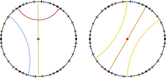
Figure 2. At left, three chordal curves $a,b,c$ on $\Sigma_{5,1}$ of types $p,q,r$, respectively. At right, two curves $d,e$ that are not chordal. $d$ is not chordal because it cannot be represented as a single segment on $D$, and $e$ is not chordal because it passes through the marked point $x$.

$c$ at 115 145 $\alpha_{5}^{2}(c)$ at 60 100 $\alpha_{5}^{4}(c)$ at 140 100 $d$ at 105 40

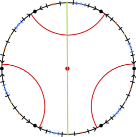
Figure 3. The curves $c,\alpha_{g}^{2}(c),\alpha_{g}^{4}(c),d$ of Lemma 3.2, illustrated for $g=5$.

An individual basic chordal curve is not (in general) invariant under nontrivial powers of $\alpha_{g}$. Lemma 3.2 shows that nevertheless, by using both $C(\alpha_{g}^{2})$ and $C(\alpha_{g}^{3})$, the symmetry can be broken and the associated Dehn twists can be exhibited as elements of $\Gamma$.

Lemma 3.2.

Let $c$ be a basic chordal curve of type $p$ or $r$. If $g\geq 3$, then $T_{c}\in\Gamma$.

Proof.

If $c$ is of type $r$, then $c$ can be represented as a diameter of $D$ and hence $c\in C(\alpha_{g}^{3})\leq\Gamma$. Suppose now that $c$ is of type $p$, connecting edges $e_{1},e_{2}$ of $\partial D$ of type $p$. In each of the model surfaces, if $g\geq 3$, then between $e_{1}$ and $e_{2}$ is an edge $e_{3}$ of type $r$ (see Figure 3). Consider the associated basic chordal curve $d$ of type $r$. As discussed above, $T_{d}\in\Gamma$, and also

$$T_{c}T_{\alpha_{g}^{2}(c)}T_{\alpha_{g}^{4}(c)}\in C(\alpha_{g}^{2})\leq\Gamma.$$

By construction, the geometric intersection $i(c,d)=1$, while also

$$i(\alpha_{g}^{2}(c),d)=i(\alpha_{g}^{4}(c),d)=0.$$

Thus,

$$(T_{c}T_{\alpha_{g}^{2}(c)}T_{\alpha_{g}^{4}(c)})T_{d}(T_{c}T_{\alpha_{g}^{2}(c)}T_{\alpha_{g}^{4}(c)})^{-1}=T_{c}T_{d}T_{c}^{-1}\in\Gamma.$$

On the other hand, since $i(c,d)=1$, the braid relation implies that

$$T_{c}T_{d}T_{c}^{-1}=T_{d}^{-1}T_{c}T_{d}\in\Gamma,$$

and hence $T_{c}\in\Gamma$ as well. ∎

3.2. $D$-convexity

The second piece of hyperbolic geometry we borrow is the notion of convexity. In the proof of Theorem 1.5, we will proceed inductively, showing that $\Gamma$ contains the mapping class groups for an increasing union of subsurfaces. In the inductive step, we will need to control the topology of the enlarged subsurface relative to the original; we accomplish this by restricting our attention to subsurfaces that are convex from the point of view of the hyperbolic metric on $\mathbb{D}^{2}$.

Definition 3.3 ($D$-convex hull, $D$-convexity).

Let $\mathcal{C}=\{c_{1},\dots,c_{n}\}$ be a collection of simple closed curves on $\Sigma_{g,1}$. Represent each $c_{i}$ as a union of chords on $D$, i.e. as a union of geodesics on the hyperbolic disk $\mathbb{D}^{2}$. The $D$-convex hull of $\mathcal{C}$ is the subsurface $\operatorname{Hull}(\mathcal{C})\subseteq\Sigma_{g,1}$ constructed as follows: first, take a closed regular neighborhood of $\bigcup c_{i}$ (viewed as a subset of $D$), take the convex hull of this set in the hyperbolic metric on $\mathbb{D}^{2}$, project onto $\Sigma_{g,1}$, and then fill in any inessential boundary components.

A subsurface $S\subset\Sigma_{g,1}$ is said to be $D$-convex if it can be represented as a convex region on $D$ with respect to the hyperbolic metric on $\mathbb{D}^{2}$.

Lemma 3.4.

Let $\mathcal{C}_{g}$ denote the set of basic chordal curves of type $p$ and $r$ on $\Sigma_{g,1}$. Then $\operatorname{Hull}(\mathcal{C}_{g})=\Sigma_{g,1}$ for all $g\geq 2$.

Proof.

For $g\equiv 1\pmod{3}$ this is clear from inspection of Figure 1, since there are no edges of type $q$ at all; the case $g=3$ similarly follows by inspection of Figure 6. For $g\equiv 2\pmod{3}$, this is best seen by inspecting Figure 4. Here one must observe that the remaining boundary components $d_{1}$ and $d_{2}$ are in fact also both inessential and hence are filled in when constructing $\operatorname{Hull}(\mathcal{C}_{g})$. For $g>3$ and $g\equiv 0\pmod{3}$, there is also exactly one family of edges of type $q$, and the same considerations as in the case $g\equiv 2\pmod{3}$ apply here as well. ∎

$A$ [bl] at 127.55 192.74 $A$ [tl] at 178.57 45.35 $B$ [tl] at 161.56 25.51 $B$ [tr] at 8.50 56.69 $C$ [tr] at 0.00 79.36 $C$ [b] at 104.87 198.41 $D$ [br] at 34.01 172.90 $D$ [bl] at 189.90 141.72 $E$ [bl] at 195.57 119.04 $E$ [tl] at 87.87 0.00 $F$ [tl] at 63.03 5.67 $F$ [bl] at 12.01 155.89 $d_{1}$ [tr] at 110.54 178.57 $d_{1}$ [bl] at 19.84 73.69 $d_{1}$ [br] at 158.73 45.35 $d_{2}$ [tr] at 175.73 124.71 $d_{2}$ [tl] at 39.68 153.06 $d_{2}$ [bl] at 82.20 19.84

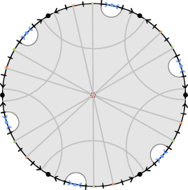
Figure 4. The final step in constructing $\operatorname{Hull}(\mathcal{C}_{g})$ for $g=5$. The boundary components $d_{1}$ and $d_{2}$ are both inessential in $\Sigma_{g,1}$ and so are filled in when constructing $\operatorname{Hull}(\mathcal{C}_{g})$.

4. proof of Theorem 1.5

We prove Theorem 1.5 in Section 4.2. The argument is inductive: we construct a sequence $S_{0}\subset S_{1}\subset\dots\subset S_{k}=\Sigma_{g,1}$ of subsurfaces and show that $\operatorname{Mod}(S_{i})\leq\Gamma$ for $i=1,\dots,k$. The inductive step is fairly simple and relies on the notion of a “stabilization” of subsurfaces to be discussed in Section 4.1. We consider separate base cases for the regimes $g\geq 4,g=3$, and $g=2$; these arguments are deferred to Sections 4.3 – 4.5.

4.1. Stabilizations

Definition 4.1 (Stabilization).

Let $S\subset\Sigma$ be a subsurface, and let $c\subset\Sigma$ be a simple closed curve such that $c\cap S$ is a single arc (the endpoints of $c$ do not necessarily lie on distinct boundary components of $S$). The stabilization of $S$ along $c$ is the subsurface $S^{+}$ constructed as a regular neighborhood of $S\cup c$ inside $\Sigma$.

Stabilizations are useful because they allow for simple inductive generating sets for the associated mapping class groups.

Lemma 4.2 (Stabilization).

Let $S\subset\Sigma$ be a subsurface of genus at least $2$, and let $S^{+}$ denote the stabilization of $S$ along the simple closed curve $c$. Then

$$\operatorname{Mod}(S^{+})=\langle T_{c},\operatorname{Mod}(S)\rangle.$$

Proof.

There are two cases to consider: either $c$ enters and exits $S$ via the same boundary component, or else it enters along one component of $\partial S$ and exits along a distinct component. In the former, $S^{+}$ has the same genus as $S$ but gains an additional boundary component, and in the latter, $S^{+}$ has genus $g(S)+1$ but one fewer boundary component. In either case, the change–of–coordinates principle for $S$ implies that $c$ can be extended to a configuration of curves $c_{0}=c,\dots,c_{n}$ such that $c_{i}\subset S$ for $i>0$ and such that the associated twists generate $\operatorname{Mod}(S^{+})$. For instance, one can take $c_{0},\dots,c_{n}$ to be the Humphries generating set for $S^{+}$ and $c_{1},\dots,c_{n}$ to be the Humphries generating set for $S$, so long as $g(S)\geq 2$. The result follows. ∎

4.2. Proof of Theorem 1.5

The result for $g=2$ will be established by separate methods in Section 4.5; we therefore assume $g\geq 3$. We will express $\Sigma_{g,1}$ as a sequence

$$S_{0}\subset S_{1}\subset\dots\subset S_{k}=\Sigma_{g,1}$$

of stabilizations of $S$ along curves in the set $\mathcal{C}_{g}$ of basic chordal curves of type $p$ and $r$. At each stage we will see that $\operatorname{Mod}(S_{i})\leq\Gamma$.

The base case. In Sections 4.3 and 4.4, we will establish the following lemma.

Lemma 4.3.

For each of the model surfaces shown in Figure 1 (excluding $g=2$) as well as the model surface in genus $3$ shown in Figure 6, there is a $D$-convex subsurface $S_{0}\subset\Sigma_{g,1}$ of genus $2$ such that $\operatorname{Mod}(S_{0})\leq\Gamma$.

The inductive step. Suppose that $S_{i}$ is given as a $D$-convex subsurface with $\operatorname{Mod}(S_{i})\leq\Gamma$. Suppose first that every curve $c_{j}\in\mathcal{C}_{g}$ is contained in $S_{i}$. Since $S_{i}$ is $D$-convex and the $D$-convex hull of $\mathcal{C}_{g}$ is $\Sigma_{g,1}$ by Lemma 3.4, in this case $S_{i}=\Sigma_{g,1}$ and the theorem is proved.

Otherwise, select $c_{j}\in\mathcal{C}_{g}$ a curve not entirely contained in $S_{i}$. We then define $S_{i+1}$ to be the $D$-convex hull of $S_{i}\cup c_{j}$. Since $S_{i}$ is $D$-convex and $c_{j}$ is a basic chordal curve, necessarily $c_{j}$ enters and exits $S_{i}$ exactly once, and hence $S_{i+1}$ is the stabilization of $S_{i}$ along $c_{j}$. By Lemma 3.2, $T_{c_{j}}\in\Gamma$, and by hypothesis, $\operatorname{Mod}(S_{i})\leq\Gamma$. By the stabilization lemma (Lemma 4.2), therefore $\operatorname{Mod}(S_{i+1})\leq\Gamma$ as well.∎

4.3. Proof of Lemma 4.3 for $g\geq 4$

$c_{1}$ [br] at 120 140 $c_{2}$ [bl] at 100 110 $c_{3}$ [br] at 120 50 $c_{4}$ [br] at 140 75 $c_{5}$ [tr] at 90 37 $S_{0}$ at 80 100

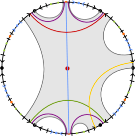
Figure 5. For $g\equiv 1\pmod{3}$, the surface $S_{0}$ is taken as the $D$-convex hull of the curves $c_{1},\dots,c_{5}$ as shown.

We will describe a chain of five curves $c_{1},\dots c_{5}$ such that $c_{1}\cup c_{3}\cup c_{5}$ bounds a pair of pants. Such a configuration is supported on a surface $S_{0}$ of genus $2$ with one boundary component, and the associated Dehn twists form the Humphries generating set for $\operatorname{Mod}(S_{0})$. The curves we will describe will either be of type $p$ (hence in $\Gamma$ by Lemma 3.2) or else invariant under $\alpha_{g}^{3}$ (and hence in $C(\alpha_{g}^{3})\leq\Gamma$). Such a configuration is illustrated in Figure 5 in the case of $g\equiv 1\pmod{4}$, but the construction we describe below works on all the model surfaces.

Let $c_{1}$ be the curve of type $p$ connecting the edges of type $p$ labeled $1$ in Figure 1. We take $c_{3}=\alpha_{g}^{3}(c_{1})$ and $c_{4}=\alpha_{g}^{4}(c_{1})$. Let $c_{2}$ be the curve of type $r$ intersecting $c_{1}$ and $c_{3}$. Finally, let $c_{5}$ be the curve obtained by connect-summing $c_{1}$ and $c_{3}$ along one of the segments of $c_{2}$. As shown in Figure 5, $c_{5}$ is invariant under $\alpha_{g}^{3}$ as required.

We find that $c_{1},c_{3},c_{4}$ are curves of type $p$, and $c_{2},c_{5}$ are invariant under $\alpha_{g}^{3}$, so all associated twists are elements of $\Gamma$, and hence $\operatorname{Mod}(S_{0})\leq\Gamma$ as claimed. ∎

4.4. Proof of Lemma 4.3 for $g=3$

$c_{1}$ [br] at 104.71 130.38 $c_{2}$ [bl] at 110.54 39.68 $c_{3}$ [bl] at 51.02 59.52 $c_{4}$ [b] at 19.84 104.87 $c_{5}$ [tl] at 39.68 99.20 $c_{6}$ [tr] at 82.20 113.38 $1$ [bl] at 155.89 175.73 $6$ [bl] at 136.05 187.07 $6$ [br] at 59.52 187.07 $5$ [br] at 39.68 175.73 $5$ [br] at 0.00 107.71 $4$ [tr] at 0.00 85.03 $4$ [tr] at 39.68 19.84 $3$ [tr] at 59.52 8.50 $3$ [tl] at 136.05 8.50 $2$ [tl] at 158.73 19.84 $2$ [tl] at 195.57 85.03 $1$ [bl] at 195.57 110.54 $x$ [tr] at 144.55 175.73 $S_{0}^{\prime}$ at 80 80 $S_{0}$ at 290 80

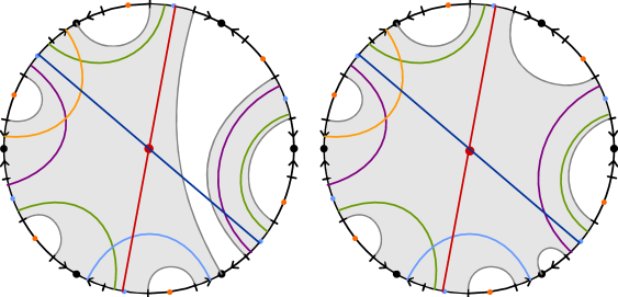
Figure 6. The model surface for $g=3$, built from the monodromy tuple $1\ 5\ 3^{2}$. The surface $S^{\prime}_{0}$ is taken as a regular neighborhood of the curves $c_{1},\dots,c_{5}$ as shown, and then $S_{0}$ is the $D$-convex hull of $c_{1},\dots,c_{6}$.

Recall from (2) that the monodromy tuple for $g=3$ is $1\ 5\ 3^{2}$. The model surface for this tuple is shown in Figure 6. To establish Lemma 4.3 in this case, we first consider the subsurface $S^{\prime}_{0}$ shown at left in Figure 6. By construction $S^{\prime}_{0}$ is a regular neighborhood of $c_{1},\dots,c_{5}$. Observe that $c_{1}$ and $c_{5}$ are $\alpha_{g}^{3}$-invariant, $c_{3}$ is $\alpha_{g}^{2}$-invariant, and $c_{2}$ and $c_{4}$ are basic chordal curves of type $p$. Thus each associated Dehn twist is an element of $\Gamma$. As above, $T_{c_{1}},\dots,T_{c_{5}}$ determines the Humphries generating set for $S^{\prime}_{0}$, and we conclude that $\operatorname{Mod}(S^{\prime}_{0})\leq\Gamma$.

We next consider $S_{0}$. By construction, $S_{0}$ is the $D$-convex hull of $c_{1},\dots,c_{6}$, and it is also clear that $S_{0}$ is the stabilization of $S^{\prime}_{0}$ along $c_{6}$. Since $c_{6}$ is a basic chordal curve of type $r$, we have $T_{c_{6}}\in\Gamma$ by Lemma 3.2. By the stabilization lemma (Lemma 4.2), it follows that $\operatorname{Mod}(S_{0})\leq\Gamma$ as required.∎

4.5. Proof of Theorem 1.5 for $g=2$

$c_{1}$ [tr] at 113.38 99.20 $c_{2}$ [t] at 85.03 116.21 $c_{3}$ [tl] at 53.85 99.20 $c_{4}$ [bl] at 53.85 65.19 $c_{5}$ [b] at 85.03 48.18 $c_{6}$ [br] at 113.38 65.19

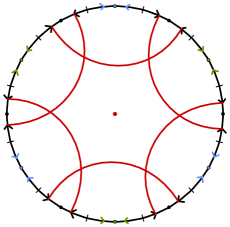
Figure 7. The model surface for $g=2$ and the curves $c_{1},\dots,c_{6}$.

For $g=2$, we take a different approach based around an explicit factorization of $\alpha_{2}$ into Dehn twists. The model for $g=2$ is shown in Figure 7. For ease of notation, we write $T_{i}$ in place of $T_{c_{i}}$ throughout the argument. The mapping class group is generated by the twists $T_{i}$ for $i=1,\dots,5$; we will show that all $T_{i}\in\Gamma$. The fundamental observation is that

$$\alpha_{2}=T_{1}T_{2}T_{3}T_{4}T_{5}.$$

We also observe that

$$T_{1}T_{4},\ T_{2}T_{5},\ T_{3}T_{6}\in\Gamma$$

since these pairs of curves are invariant under $\alpha_{2}^{3}$, and also

$$T_{1}T_{3}T_{5},\ T_{2}T_{4}T_{6}\in\Gamma$$

since these triples are invariant under $\alpha_{2}^{2}$.

We consider the expression of elements of $\Gamma$

$$\alpha_{2}(T_{2}T_{5})^{-1}(T_{1}T_{4})^{-1} =T_{1}T_{2}T_{3}T_{4}T_{5}T_{5}^{-1}T_{2}^{-1}T_{4}^{-1}T_{1}^{-1}$$

$$=T_{1}T_{2}T_{3}T_{2}^{-1}T_{1}^{-1},$$

with the second equality holding by the commutativity of $T_{i}$ and $T_{j}$ whenever $i\neq j\pm 1$. Conjugating $T_{1}T_{2}T_{3}T_{2}^{-1}T_{1}^{-1}$ by $(T_{1}T_{3}T_{5})^{-1}$ shows that the element

$$(T_{1}T_{3}T_{5})^{-1}T_{1}T_{2}T_{3}T_{2}^{-1}T_{1}^{-1}(T_{1}T_{3}T_{5})=T_{3}^{-1}T_{2}T_{3}T_{2}^{-1}T_{3}$$

is also in $\Gamma$. Conjugating this by $(T_{3}T_{6})$ shows that

$$T_{2}T_{3}T_{2}^{-1}\in\Gamma;$$

a final conjugation by $(T_{2}T_{5})^{-1}$ reveals that $T_{3}\in\Gamma$. Conjugation by $\alpha_{2}$ now exhibits all $T_{i}$ in $\Gamma$. ∎

5. Mapping class group actions on $\mathbb{R}^{3}$

In this final section, we show how Theorem 1.5 implies Theorem 1.3 and Corollary 1.4. Recall that the objective is to show that for $g\geq 4$, any action of $\operatorname{Mod}(\Sigma_{g,1})$ on $\mathbb{R}^{3}$ has a globally-invariant line, and consequently that $\operatorname{Mod}(\Sigma_{g,1})$ does not act by $C^{1}$ diffeomorphisms on $\mathbb{R}^{2}$ or $\mathbb{R}^{3}$.

We consider an action $\rho$ of $\operatorname{Mod}(\Sigma_{g,1})$ on $\mathbb{R}^{3}$. Recall that any such action must necessarily preserve orientation. We will appeal to the following result of Lanier–Margalit [6, Theorem 1.1].

Theorem 5.1 (Lanier–Margalit).

For $g\geq 3$, every nontrivial periodic mapping class that is not hyperelliptic normally generates $\operatorname{Mod}(\Sigma_{g,1})$ or $\operatorname{Mod}(\Sigma_{g})$.

We remark that [6, Theorem 1.1] only discusses the case $\operatorname{Mod}(\Sigma_{g})$, however the same method applies to $\operatorname{Mod}(\Sigma_{g,1})$.

By Theorem 5.1, $\alpha_{g}^{2}$ normally generates $\operatorname{Mod}(\Sigma_{g,1})$. Therefore if $\rho$ is not trivial, then $\rho(\alpha_{g}^{2})$ is not trivial. By local Smith theory ([1, Theorem 20.1]), the fixed point set of $\alpha_{g}^{2}$ is a $\mathbb{Z}/3\mathbb{Z}$–homology manifold of dimension less than $2$. By [1, Theorem 16.32], when the dimension of a homology manifold is less than $2$, it is a topological manifold. We claim that the fixed set $F(\alpha_{g}^{2})$ of $\rho(\alpha_{g}^{2})$ is a single topological line in $\mathbb{R}^{3}$. Since $\mathbb{R}^{3}$ is acyclic, also $F(\alpha_{g}^{2})$ is also acyclic (c.f. [1, Corollary 19.8]). Hence $F(\alpha_{g}^{2})$ must have exactly one component. By [1, Corollary 19.11], $F(\alpha_{g}^{2})$ is a line, since we can consider the action on the one-point compactification of $\mathbb{R}^{3}$. This can be compared with the fact that the fixed set of a torsion element in $SO(3)$ is a single line in $\mathbb{R}^{3}$.

Since $\alpha_{g}^{3}$ is not hyperelliptic, the same argument shows that the fixed set of $\rho(\alpha^{3})$ is also a line $F(\alpha_{g}^{3})$. We claim that $F(\alpha_{g}^{2})=F(\alpha_{g}^{3})$, which will be denoted by $F$. If these lines are distinct, then the action of $\rho(\alpha_{g})$ on $F(\alpha_{g}^{3})$ must be nontrivial (otherwise $\rho(\alpha_{g}^{2})$ would act trivially as well, implying $F(\alpha_{g}^{2})=F(\alpha_{g}^{3})$). As $\rho(\alpha_{g}^{3})$ acts trivially on $F(\alpha_{g}^{3})$ by construction, it follows that $\rho(\alpha_{g})$ acts as an element of order $3$. This is a contradiction: there is no nontrivial action of $\mathbb{Z}/3\mathbb{Z}$ on a line. Thus by Theorem 1.5, $\operatorname{Mod}(\Sigma_{g,1})$ must preserve $F$, establishing Theorem 1.3.

Now suppose $\rho$ acts by $C^{1}$ diffeomorphisms, and let $x\in F$ be any fixed point. Taking derivatives at $x$, we obtain a representation $R:\operatorname{Mod}(\Sigma_{g,1})\to\operatorname{GL}(3,\mathbb{R})$. According to [4, Theorem 1.1], any such homomorphism is trivial. The Thurston stability theorem [9] then implies that the image of $\rho$ must be locally-indicable, i.e. every finitely-generated subgroup admits a surjection onto $\mathbb{Z}$. In particular, $\text{im}(\rho)$ must be torsion-free, and so $\rho(\alpha_{g})$ is the identity map. By Theorem 5.1, it follows that the entire representation $\rho$ is trivial.∎

Remark.

In fact, the conclusions of Theorem 1.3 and Corollary 1.4 hold for $g=3$ as well, using slightly different arguments. We briefly discuss this. From the discussion above, if $\rho(\alpha_{g}^{3})$ is not trivial, the same arguments apply. Otherwise, denote by $H:\operatorname{Mod}(S_{g,1})\to\text{Sp}(2g,\mathbb{Z})$ the induced action on $H_{1}(S_{g};\mathbb{Z})$. If $\alpha_{g}^{3}$ is hyperelliptic and $\rho(\alpha_{g}^{3})$ is the identity, we claim that $\rho$ factors through $H$. This is because the hyperelliptic involution $\alpha_{g}^{3}$ normally generates the group $H^{-1}(\pm I)$ by [6, Proposition 3.3], whose proof also works for the punctured case.

To conclude, we claim that there is no action of $\text{Sp}(2g,\mathbb{Z})$ on $\mathbb{R}^{3}$, even by homeomorphisms. According to [11, Corollary 1], $(\mathbb{Z}/3\mathbb{Z})^{3}$ is not a subgroup of $\text{Homeo}(\mathbb{R}^{3})$. The claim then follows from [3, Lemma 10].

References

- Bre [97] G. Bredon. Sheaf theory, volume 170 of Graduate Texts in Mathematics. Springer-Verlag, New York, second edition, 1997.
- CK [94] A. Constantin and B. Kolev. The theorem of Kerékjártó on periodic homeomorphisms of the disc and the sphere. Enseign. Math., 40:193–193, 1994.
- CL [20] L. Chen and J. Lanier. Constraining mapping class group homomorphisms using finite subgroups. Preprint, 2020.
- FH [13] J. Franks and M. Handel. Triviality of some representations of in , and . Proc. Amer. Math. Soc., 141(9):2951–2962, 2013.
- Kir [78] R. Kirby. Problems in low dimensional manifold theory. In Algebraic and geometric topology (Proc. Sympos. Pure Math., Stanford Univ., Stanford, Calif., 1976), Part 2, Proc. Sympos. Pure Math., XXXII, pages 273–312. Amer. Math. Soc., Providence, R.I., 1978.
- LM [18] J. Lanier and D. Margalit. Normal generators for mapping class groups are abundant. Preprint: https://arxiv.org/abs/1805.03666, 2018.
- Mar [07] V. Markovic. Realization of the mapping class group by homeomorphisms. Invent. Math., 168(3):523–566, 2007.
- MT [18] K. Mann and B. Tshishiku. Realization problems for diffeomorphism groups. Preprint: https://arxiv.org/abs/1802.00490, 2018.
- Thu [74] W. P. Thurston. A generalization of the Reeb stability theorem. Topology, 13:347–352, 1974.
- vK [19] B. von Kerékjártó. Über die periodischen Transformationen der Kreisscheibe und der Kugelfläche. Math. Ann., 80(1):36–38, 1919.
- Zim [18] B. Zimmermann. On topological actions of finite groups on . Topology Appl., 236:59–63, 2018.