Talking-Heads Attention
 

Abstract

We introduce "talking-heads attention" - a variation on multi-head attention which includes linear projections across the attention-heads dimension, immediately before and after the softmax operation. While inserting only a small number of additional parameters and a moderate amount of additional computation, talking-heads attention leads to better perplexities on masked language modeling tasks, as well as better quality when transfer-learning to language comprehension and question answering tasks.

1 Introduction

Neural Attention was introduced by [Bahdanau et al., 2014] as a way of extracting information from variable-length representations. The Transformer model [Vaswani et al., 2017] uses "multi-head" attention, consisting of multiple attention layers ("heads") in parallel, each with different projections on its inputs and outputs. By using a dimensionality reduction in the input projections, the computational cost is kept similar to that of basic attention. Quality is improved, presumably due to the ability to attend to multiple positions simultaneously based on multiple different types of relationships.

As noted in [Vaswani et al., 2017], taking this process to the extreme (more attention heads projected to lower dimensionality) becomes counterproductive. We believe that this is due to the fact that the query-vectors and key-vectors become so low-dimensional that their dot product can no longer constitute an informative matching function.

In this paper, we introduce a new variant, "talking-heads attention", that addresses this problem by inserting a learned linear projection across the attention-heads dimension of the attention-logits tensor. This allows each attention function to depend on all of the keys and queries. We also insert a second such projection immediately following the softmax.

We show experimentally that inserting these "talking-heads" projections leads to better perplexities on masked language modeling tasks, as well as better quality when transfer-learning to language comprehension and question answering tasks.

2 Notation

In our pseudocode, we use capital letters to represent tensors and lower-case letters to represent their dimensions. Each tensor is followed by a dimension list in brackets. For example, a 4-dimensional image-tensor with (batch, height, width, channels) dimensions would be written as:

⬇

X[b, h, w, c]

We use einsum notation for generalized contractions between tensors of arbitrary dimension. The computation is numerically equivalent to broadcasting each input to have the union of all dimensions, multiplying component-wise, and summing across all dimensions not in the output. Rather than identifying the dimensions by an equation, as in TensorFlow and numpy, the dimensions are indentified by the dimension-list annotations on the arguments and on the result. For example, multiplying two matrices would be expressed as:

⬇

Y[a, c] = einsum(X[a, b], W[b, c])

3 Review of Attention Algorithms

3.1 Dot-Product Attention

Simple dot-product attention can be described by the pseudocode below. The logits L are computed as the dot-products of the query-vectors and the memory-vectors. For each query, the logits are passed through a softmax function to produce weights, and the different memory-vectors are averaged together, weighted by those weights. In this code, we show the case where there are $n$ different queries all attending to the same $m$ memory-vectors. If there is only one query, the code is identical except that the "n" dimension is removed from all tensors.
⬇ def DotProductAttention( X[n, d], # n query-vectors with dimensionality d M[m, d]): # m memory-vectors with dimensionality d L[n, m] = einsum(X[n, d], M[m, d]) # Attention logits W[n, m] = softmax(L[n, m], reduced_dim=m) # Attention weights Y[n, d] = einsum(W[n, m], M[m, d]) return Y[n, d]

3.2 Dot-Product Attention With Projections

[Vaswani et al., 2017] propose a dimensionality-reduction to reduce the computational complexity of the attention algorithm. In this version, instead of computing the attention algorithm directly on the inputs $X$ and $M$, we first project the inputs using the learned linear projections $P_{q}$, $P_{k}$ and $P_{v}$, to produce lower-dimensional query-vectors, key-vectors and value-vectors $Q$, $K$ and $V$. We use a fourth learned linear projection, $P_{o}$, to produce the output.

⬇

def DotProductAttentionWithProjections(

X[n, d_X], # n vectors with dimensionality d_X

M[m, d_M], # m vectors with dimensionality d_M

P_q[d_X, d_k], # learned linear projection to produce queries

P_k[d_M, d_k], # learned linear projection to produce keys

P_v[d_M, d_v], # learned linear projection to produce values

P_o[d_Y, d_v]): # learned linear projection of output

Q[n, d_k] = einsum(X[n, d_X], P_q[d_X, d_k]) # queries

K[m, d_k] = einsum(M[m, d_M], P_k[d_M, d_k]) # keys

V[m, d_v] = einsum(M[m, d_M], P_v[d_M, d_v]) # values

L[n, m] = einsum(Q[n, d_k], K[m, d_k]) # Attention logits

W[n, m] = softmax(L[n, m], reduced_dim=m) # Attention weights

O[n, d_v] = einsum(W[n, m], V[m, d_v])

Y[n, d_Y] = einsum(O[n, d_v], P_o[d_Y, d_v])

return Y[n, d_Y]

3.3 Multi-Head Attention

The multi-head attention described in [Vaswani et al., 2017] consists of the sum of multiple parallel attention layers. This can be represented by adding a "heads" dimension h to the above computation.
⬇ def MultiHeadAttention( X[n, d_X], # n vectors with dimensionality d_X M[m, d_M], # m vectors with dimensionality d_M P_q[d_X, d_k, h], # learned linear projection to produce queries P_k[d_M, d_k, h], # learned linear projection to produce keys P_v[d_M, d_v, h], # learned linear projection to produce values P_o[d_Y, d_v, h]): # learned linear projection of output Q[n, d_k, h] = einsum(X[n, d_X], P_q[d_X, d_k, h]) # queries h*n*d_X*d_k K[m, d_k, h] = einsum(M[m, d_M], P_k[d_M, d_k, h]) # keys h*m*d_M*d_k V[m, d_v, h] = einsum(M[m, d_M], P_v[d_M, d_v, h]) # values h*m*d_M*d_v L[n, m, h] = einsum(Q[n, d_k, h], K[m, d_k, h]) # logits h*n*m*d_k W[n, m, h] = softmax(L[n, m, h], reduced_dim=m) # weights O[n, d_v, h] = einsum(W[n, m, h], V[m, d_v, h]) # h*n*m*d_v Y[n, d_Y] = einsum(O[n, d_v, h], P_o[d_Y, d_v, h]) # output h*n*d_Y*d_v return Y[n, d_Y]

The pseudo-code above illustrates the practical step-by-step computation of multi-head attention. The costs of the einsum operations (the number of multiplications in a naive implementation) are shown in the comments. The equivalent pseudo-code below uses multi-way einsums and is more concise:
⬇ def MultiHeadAttentionConcise(X, M, P_q, P_k, P_v, P_o): L[n, m, h] = einsum(X[n, d_X], M[m, d_M], P_q[d_X, d_k, h], P_k[d_M, d_k, h]) W[n, m, h] = softmax(L[n, m, h], reduced_dim=m) Y[n, d] = einsum(W[n, m, h], M[m, d_M], P_v[d_M, d_v, h], P_o[d_Y, d_v, h]) return Y[n, d_Y]

Note: [Vaswani et al., 2017] include a constant scaling factor on the logits. We omit this in our code, as it can be folded into the linear projections $P_{q}$ or $P_{k}$.

4 Talking-Heads Attention

In multi-head attention, the different attention heads perform separate computations, which are then summed at the end. Our new variation, which we call "Talking-Heads Attention" breaks that separation. We insert two additional learned linear projections, ${P_{l}}$ and ${P_{w}}$, which transform the attention-logits and the attention-weights respectively, moving information across attention heads. Instead of one "heads" dimension $h$ across the whole computation, we now have three separate heads dimensions: $h_{k}$, $h$, and $h_{v}$, which can optionally differ in size (number of "heads"). $h_{k}$ refers to the number of attention heads for the keys and the queries. $h$ refers to the number of attention heads for the logits and the weights, and $h_{v}$ refers to the number of attention heads for the values. The algorithm is shown by the pseudo-code below. The costs of the einsum operations are shown in the comments.
⬇ def TalkingHeadsAttention( X[n, d_X], # n vectors with dimensionality d_X M[m, d_M], # m vectors with dimensionality d_M P_q[d_X, d_k, h_k], # learned linear projection to produce queries P_k[d_M, d_k, h_k], # learned linear projection to produce keys P_v[d_M, d_v, h_v], # learned linear projection to produce values P_o[d_Y, d_v, h_v], # learned linear projection of output P_l[h_k, h], # talking-heads projection for logits P_w[h, h_v]): # talking-heads projection for weights Q[n, d_k, h_k] = einsum(X[n, d_X], P_q[d_X, d_k, h_k]) # queries n*d_X*d_k*h_k K[m, d_k, h_k] = einsum(M[m, d_M], P_k[d_M, d_k, h_k]) # keys m*d_M*d_k*h_k V[m, d_v, h_v] = einsum(M[m, d_M], P_v[d_M, d_v, h_v]) # values m*d_M*d_v*h_v J[n, m, h_k] = einsum(Q[n, d_k, h_k], K[m, d_k, h_k]) # dot prod. n*m*d_k*h_k L[n, m, h] = einsum(J[n, m, h_k], P_l[h_k, h]) # Talking-heads proj. n*m*h*h_k W[n, m, h] = softmax(L[n, m, h], reduced_dim=m) # Attention weights U[n, m, h_v] = einsum(W[n, m, h], P_w[h, h_v]) # Talking-heads proj. n*m*h*h_v O[n, d_v, h_v] = einsum(U[n, m, h_v], V[m, d_v, h_v]) # n*m*d_v*h_v Y[n, d_Y] = einsum(O[n, d_v, h_v], P_o[d_Y, d_v, h_v]) # n*d_Y*d_v*h_v return Y[n, d_Y] Again, we can write this more concisely using multi-way einsum operations:
⬇ def TalkingHeadsAttentionConcise(X, M, P_q, P_k, P_v, P_o, P_l, P_w): L[n, m, h] = einsum(X[n, d_X], M[m, d_M], P_q[d_X, d_k, h_k], P_k[d_M, d_k, h_k], P_l[h_k, h]) W[n, m, h] = softmax(L[n, m, h], reduced_dim=m) Y[n, d_Y] = einsum(W[n, m, h], M[m, d_M], P_v[d_M, d_v, h_v], P_o[d_Y, d_v, h_v], P_w[h, h_v]) return Y[n, d_Y]

5 Complexity Analysis

If we assume that $d_{X}=d_{Y}$, then the number of scalar multiplications in multi-head attention is:

$$h\cdot(d_{k}+d_{v})\cdot(n\cdot d_{X}+m\cdot d_{M}+n\cdot m)$$

The number of scalar multiplications in talking-heads attention is:

$$(d_{k}\cdot h_{k}+d_{v}\cdot h_{v})\cdot(n\cdot d_{X}+m\cdot d_{M}+n\cdot m)+n\cdot m\cdot h\cdot(h_{k}+h_{v})$$

The first term in this expression matches up with the cost of multi-head attention. The second term is due to the talking-heads projections. If $h<d_{k}$ and $h<d_{v}$, the the costs of the new talking-heads projections, $n\cdot m\cdot h\cdot h_{k}$ and $n\cdot m\cdot h\cdot h_{v}$ are less than the existing terms $n\cdot m\cdot d_{k}\cdot h_{k}$ and $n\cdot m\cdot d_{v}\cdot h_{v}$, respectively.

In practice, the talking-heads projections may be expensive on some neural-network accelerators due to the small dimension sizes involved.

6 One More Way To Look At It

Mathematically, one can view multi-head attention and talking-heads attention as two special cases of the same general function, which we will call "general bilinear multihead attention" (GBMA). GBMA uses two three-dimensional parameter tensors, as defined in the pseudocode below. Due to its high computational cost, GBMA may have no practical use. Multi-head attention is mathematically equivalent to a version of GBMA where each of the two parameter tensors is expressed as the product of two factors, as shown below. Talking-heads attention is mathematically equivalent to a version of GBMA where each of the two parameter tensors is expressed as the product of three factors, as shown below.
⬇ def GeneralBilinearMultiheadAttention( X[n, d_X], # n vectors with dimensionality d_X M[m, d_M], # m vectors with dimensionality d_M P[d_X, d_M, h], # learned parameters Q[d_M, d_Y, h]): # learned parameters L[n, m, h] = einsum(X[n, d_X], M[m, d_M], P[d_X, d_M, h]) W[n, m, h] = softmax(L[n, m, h], reduced_dim=m) Y[n, d_Y] = einsum(W[n, m, h], M[m, d_M], Q[d_M, d_Y, h]) return Y[n, d_Y] def MultiHeadAttentionInefficient(X, M, P_q, P_k, P_v, P_o): P[d_X, d_M, h] = einsum(P_q[d_X, d_k, h], P_k[d_M, d_k, h]) Q[d_M, d_Y, h] = einsum(P_v[d_M, d_v, h], P_o[d_Y, d_v, h]) return GeneralBilinearMultiheadAttention(X, M, P, Q) def TalkingHeadsAttentionInefficient(X, M, P_q, P_k, P_v, P_o, P_l, P_w): P[d_X, d_M, h] = einsum(P_q[d_X, d_k, h_k], P_k[d_M, d_k, h_k], P_l[h_k, h]) Q[d_M, d_Y, h] = einsum(P_v[d_M, d_v, h_v], P_o[d_Y, d_v, h_v], P_w[h, h_v]) return GeneralBilinearMultiheadAttention(X, M, P, Q)

7 Experiments

7.1 Text-to-Text Transfer Transformer (T5)

We test various configurations of multi-head attention and talking-heads attention on the transfer-learning setup from [Raffel et al., 2019]. An encoder-decoder transformer model [Vaswani et al., 2017] is pre-trained on a denoising objective of predicting missing text segments (average span length 3) from the C4 dataset [Raffel et al., 2019] , and subsequently fine-tuned on various language understanding tasks. We use the same code base and model architecture as the base model from [Raffel et al., 2019]. The encoder and decoder each consist of 12 layers, with $d_{model}=768$ and $d_{ff}=3072$. Each encoder layer contains a multi-head self-attention layer, and each decoder layer contains a multi-head self-attention layer and a multi-head attention-over-encoder layer. For their base model, [Raffel et al., 2019] follow [Devlin et al., 2018] and others, using $h=12$ and $d_{k}=d_{v}=64$ for all of these attention layers. We compare this setting to a variety of other configurations of multi-head and talking-heads attention, as detailed in table 1.

Similar to [Raffel et al., 2019], we pre-train our models for 524288 steps. Each training batch consists of 128 examples, each of which has an input of 512 tokens and an output of 114 tokens, the output containing multiple spans of tokens which were deleted from the input. Similarly to [Raffel et al., 2019], we use the Adafactor optimizer [Shazeer and Stern, 2018] and an inverse-square-root learning-rate schedule. We also decay the learning rate linearly for the final 10 percent of the training steps. Our main departure from [Raffel et al., 2019] is that we, as suggested by [Lan et al., 2019], use no dropout during pre-training. We find this to produce superior results. We compute the log-perplexity on the training objective on a held-out shard of C4, which we believe to be a good indicator of model quality. For each configuration, we train one model for the "full" 524288 steps and four models for a shorter time (65536 steps) to measure inter-run variability. The results are listed in table 1.

We then fine-tune each of the models on an examples-proportional mixture of SQUAD [Rajpurkar et al., 2016], GLUE [Wang et al., 2018] and SuperGlue [Wang et al., 2019]. Fine-tuning consists of 131072 additional steps with a learning rate of $10^{-3}$. Following [Raffel et al., 2019], we use a dropout rate $0.1$ on the layer outputs, feed-forward hidden-layers and attention weights. The embedding matrix (also used as the projection in the final classifier layer) is fixed during fine-tuning. Tables 1, 2, 3 and 4 include results for SQUAD and MNLI-m. Results for all other tasks are listed in the appendix.

7.1.1 Multi-Head vs Talking-Heads Attention

Table 1: Multi-Head vs. Talking-Heads attention on T5

						ln(PPL)	ln(PPL)	SQUAD		step	parameters	multiplies
						65536	524288	v1.1	MNLI-m	time	per	per att. layer
	$h_{k}$	$h$	$h_{v}$	$d_{k}$	$d_{v}$	steps	steps	dev-f1	dev	(s)	att. layer	(n=m=512)
multi-head		6		128	128	2.010 (0.005)	1.695	89.88	85.34	0.14	2359296	$1.611\cdot 10^{9}$
multi-head		12		64	64	1.982 (0.003)	1.678	90.87	86.20	0.15	2359296	$1.611\cdot 10^{9}$
multi-head		24		32	32	1.989 (0.009)	1.669	91.04	86.41	0.17	2359296	$1.611\cdot 10^{9}$
multi-head		48		16	16	2.011 (0.004)	1.682	90.35	85.32	0.21	2359296	$1.611\cdot 10^{9}$
talking-heads	6	6	6	128	128	1.965 (0.009)	1.659	90.51	85.99	0.16	2359368	$1.629\cdot 10^{9}$
talking-heads	12	12	12	64	64	1.932 (0.004)	1.641	91.38	86.19	0.18	2359584	$1.686\cdot 10^{9}$
talking-heads	24	24	24	32	32	1.910 (0.001)	1.624	91.83	87.42	0.22	2360448	$1.913\cdot 10^{9}$
talking-heads	48	48	48	16	16	1.903 (0.006)	1.603	91.90	87.50	0.32	2363904	$2.819\cdot 10^{9}$
multi-head		24		64	64	1.950 (0.005)	1.625	91.46	86.58	0.22	4718592	$3.221\cdot 10^{9}$
general bilinear		12		768	768	1.921 (0.011)	1.586	90.83	86.50	0.47	14155776	$7.650\cdot 10^{9}$
[Raffel et al., 2019]		12		64	64			89.66	84.85		2359296	$1.611\cdot 10^{9}$

In table 1, we compare multi-head attention to talking-heads attention. For each of the two algorithms, we test versions with 6, 12, 24 and 48 heads. Following [Vaswani et al., 2017], as we increase the number of heads, we decrease the key/value dimensionality $d_{k}$ and $d_{v}$, so as to keep the number of parameters constant. For each number of heads, talking-heads attention improves over multi-head attention on all quality metrics.

Additionally, multi-head attention gets worse as we increase the number of heads from 24 to 48 and decrease the key and value dimensionalty from 32 to 16, while talking-heads attention gets better. We presume that this is due to the keys being too short to produce a good matching signal.

For additional comparison, we include in table 1 two models with significantly more parameters and computation in the attention layers. In the first, we double the number of heads in our baseline model from $12$ to $24$ without reducing $d_{k}$ and $d_{v}$, resulting in a multi-head attention layer with double the parameters and double the computation. In the second, we use "general bilinear multihead attention", as described in section 6.

We also list the results from [Raffel et al., 2019]. We believe that their results are worse due to their use of dropout during pre-training.

7.1.2 Varying the Heads-Dimensions Separately

Table 2: Talking-heads attention has three "heads" dimensions that can vary independently.

						ln(PPL)	ln(PPL)	SQUAD		step	parameters	multiplies
						65536	524288	v1.1	MNLI-m	time	per	per att. layer
	$h_{k}$	$h$	$h_{v}$	$d_{k}$	$d_{v}$	steps	steps	dev-f1	dev	(s)	att. layer	(n=m=512)
talking-heads	6	6	6	128	128	1.965 (0.009)	1.659	90.51	85.99	0.16	2359368	$1.629\cdot 10^{9}$
talking-heads	6	24	6	128	128	1.941 (0.009)	1.641	90.91	86.29	0.18	2359584	$1.686\cdot 10^{9}$
talking-heads	24	6	24	32	32	1.959 (0.008)	1.667	90.77	86.15	0.20	2359584	$1.686\cdot 10^{9}$
talking-heads	6	24	24	128	32	1.939 (0.011)	1.633	91.06	86.31	0.20	2360016	$1.799\cdot 10^{9}$
talking-heads	24	24	6	32	128	1.931 (0.013)	1.628	90.98	86.81	0.21	2360016	$1.799\cdot 10^{9}$
talking-heads	24	24	24	32	32	1.910 (0.001)	1.624	91.83	87.42	0.22	2360448	$1.913\cdot 10^{9}$

In table 2, we experiment with independently varying the sizes of the three heads-dimensions. From the results, it appears that all three are good to increase, but that the softmax-heads dimension $h$ is particularly important.

7.1.3 Logits-Projection Only and Weights-Projection Only

Table 3: The logits-projection and the weights-projection can be employed separately.

						ln(PPL)	ln(PPL)	SQUAD		step	parameters	multiplies
						65536	524288	v1.1	MNLI-m	time	per	per att. layer
	$h_{k}$	$h$	$h_{v}$	$d_{k}$	$d_{v}$	steps	steps	dev-f1	dev	(s)	att. layer	(n=m=512)
multi-head		24		32	32	1.989 (0.009)	1.669	91.04	86.41	0.17	2359296	$1.611\cdot 10^{9}$
project logits	24	24		32	32	1.969 (0.004)	1.652	91.29	85.86	0.23	2359872	$1.762\cdot 10^{9}$
project weights		24	24	32	32	1.951 (0.009)	1.636	91.03	86.12	0.23	2359872	$1.762\cdot 10^{9}$
talking-heads	24	24	24	32	32	1.910 (0.001)	1.624	91.83	87.42	0.22	2360448	$1.913\cdot 10^{9}$

In the middle two experiments of table 3, we examine hybrids of multi-head attention and talking-heads attention, where there is a projection on one but not both of the logits and the weights.

7.1.4 Encoder vs. Decoder

Table 4: In each of the middle three experiments, talking-heads attention is employed in only one of the three types of attention layers in the model.

						ln(PPL)	ln(PPL)	SQUAD		step	parameters	multiplies
						65536	524288	v1.1	MNLI-m	time	per	per att. layer
	$h_{k}$	$h$	$h_{v}$	$d_{k}$	$d_{v}$	steps	steps	dev-f1	dev	(s)	att. layer	(n=m=512)
multi-head		24		32	32	1.989 (0.009)	1.669	91.04	86.41	0.17	2359296	$1.611\cdot 10^{9}$
TH-enc-self	24*	24	24*	32	32	1.969 (0.002)	1.655	91.63	87.00	0.21	various	various
TH-dec-self	24*	24	24*	32	32	1.981 (0.005)	1.671	90.56	85.56	0.17	various	various
TH-encdec	24*	24	24*	32	32	1.942 (0.003)	1.646	90.86	86.07	0.18	various	various
talking-heads	24	24	24	32	32	1.910 (0.001)	1.624	91.83	87.42	0.22	2360448	$1.913\cdot 10^{9}$

The transformer model contains three types of attention layers - self-attention in the encoder, self-attention in the decoder, and attention-over-encoder in the decoder. In each of the middle three experiments of table 4, we employ talking-heads attention in only one of these types of attention layers, and multi-head attention in the others. We find that modifying the encoder-self-attention layers has the biggest effect on the downstream language-understanding tasks. This is unsurprising, given that these tasks have more to do with analyzing the input than with generating output.

7.2 ALBERT

[Lan et al., 2019] introduce ALBERT, a variation on BERT [Devlin et al., 2018]. The main difference between the ALBERT and BERT architectures is that ALBERT shares layer parameters among all layers, significantly reducing the number of parameters. For example, a 12-layer ALBERT model has about 1/12 the number of parameters in the attention and feed-forward layers as a similar BERT model. Another difference is that the ALBERT model factorizes the word embedding as the product of two matrices with smaller bases, again significantly reducing the parameter count. This makes ALBERT appealing for memory limited devices such as mobiles. Besides above architecture differences, ALBERT also uses sentence order prediction (SOP) to replace next sentence prediction (NSP) in BERT.

We report here experiments done with the base setting for ALBERT: a Transformer network with 12 layers of attention, the hidden and embedding size set to 768. The pre-training and fine-tuning hyperparameter settings are also exactly the same as in [Lan et al., 2019]. We use the English Wikipedia and book corpus datasets [Devlin et al., 2018] to pre-train various models with different head sizes and talking-heads configurations. We evaluate the resulting representations by using them as a starting point to finetune for the SQuAD task (SQuAD1.1, SQuAD2.0 dev set) and various tasks (MNLI, SST-2, RACE) from the GLUE benchmark. Results are in Table 5.

Table 5: Multi-Head vs. Talking-Heads attention on ALBERT.

	heads	$d_{k}=d_{v}$	SQuAD1.1 (f1)	SQuAD2.0 (f1)	MNLI	SST-2	RACE	MLM	SOP	Average
Multi-head	6	128	88.5	78.8	79.9	88.6	62.7	54.3	85.9	79.7
Multi-head	12	64	88.8	79.3	80.2	89.9	63.4	54.5	86.2	80.32
Multi-head	24	32	88.8	79.1	79.9	87.7	62.1	54.4	85.9	79.52
Multi-head	48	16	87.9	78.8	79.6	88.4	61.8	53.8	85.3	79.3
Talking-heads	6	128	88.7	78	80	88.5	62	54.1	85.2	79.44
Talking-heads	12	64	89.2	79.9	80.5	89	65.3	54.9	87.6	80.78
Talking-heads	24	32	89.3	80.5	80.5	87.6	65.6	55.3	86.3	80.7
Talking-heads	48	16	89.6	80.9	80.9	89.3	66.5	55.7	86.5	81.44

We find that as the number of heads increases beyond 12 and the dimensionality of the attention-keys and attention-values decreases below 64, the performance of multi-head attention decays. On the other hand, the performance of talking-head attention keeps improving.

In addition, we also compare the logits projection and the weight projection separately with multi-head and talking-heads attention. The results are shown in Table 6. Similar to our observation in T5 experiments, only applying either the logits projection or the weight projection does not result in significant improvement compared to without them. These results again confirm the importance of having both projections.

Table 6: The logits-projection and the weights-projection can be employed separately.

	heads	$d_{k}=d_{v}$	SQuAD1.1 (f1)	SQuAD2.0 (f1)	MNLI	SST-2	RACE	MLM	SOP	Average
Multi-head	12	64	88.8	79.3	80.2	89.9	63.4	54.5	86.2	80.32
Logit-project-only	12	64	88.5	78.8	79.8	89.3	63	54.6	85.8	79.88
Weight-project-only	12	64	88.9	79.6	80.3	89	64	54.7	85.8	80.36
Talking-heads	12	64	89.2	79.9	80.5	89	65.3	54.9	87.6	80.78

7.3 BERT

We test various configurations of talking-heads attention based on [Devlin et al., 2018]. All of our experiments use the simplified relative position embeddings [Raffel et al., 2019] instead of fixed position embedding. We first pre-train a 12 Transformer layers using the same dataset as [Devlin et al., 2018]. And then we finetune for the SQuAD1.1 task and the MNLI from the GLUE dataset. Our experiments show that quality continues to improve when we grow the number of heads up to 768 and decrease the key and value dimensionality down to 1

Table 7: Talking-Heads attention on BERT.

	heads	$d_{k}=d_{v}$	SQuAD1.1 (f1)	MNLI
Multi-head	12	64	88.51	82.6
Talking-heads	6	128	88.8	83.4
Talking-heads	12	64	89.2	83.6
Talking-heads	24	32	89.4	83.6
Talking-heads	48	16	89.5	83.4
Talking-heads	64	12	89.9	83.8
Talking-heads	96	8	89.3	83.6
Talking-heads	192	4	89.8	83.9
Talking-heads	384	2	90.5	83.9
Talking-heads	768	1	90.5	84.2

7.4 Visualizing the Projection Matrices of Talking-Heads

To illustrate how different heads exchange information with each other, we visualize the projection matrices ($P_{l}$ and $P_{w}$) of a 12 layer BERT with 12 talking-heads in figure 1. Since $P_{w}$ is applied after $P_{l}$ (although there is a softmax non-linearity in between), we also visualize the combined transformation $P_{l}\times P_{w}$ in figure 1. As can be observed, the main diagonals of the projection matrices do not have significant greater values than other entries. This is expected because with talking-heads, a pair of query and key do not corresponds to any specific value-vector. All keys and queries jointly decide how the values in each head interchange data. Additionally, all projection matrices are well conditioned (magnitude of determinant above $10^{-9}$ with smallest eigenvalue above $10^{-3}$), indicating that no significant approximation can be achieved.

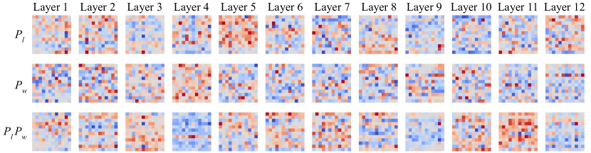
Figure 1: Visualization of the learned projection matrices $P_{l}$, $P_{w}$, and the multiplication $P_{l}\times P_{w}$. All entries in each matrix are normalized to [-1, 1]. The fact that these matrices are not diagonal or sparse at all, shows that there are significant data exchange across different attention heads.

8 Conclusions and Future Work

We have proposed talking-heads attention and shown some promising results. One potential challenge is speed on modern deep-learning accelerators, which are optimized for large-dimension matrix multiplications. We imagine that this will be an area of future work. One approach is to build hardware which is better at small-dimension matrix-multiplication. Another potential approach is to decrease the number of memory-positions considered for each query-position - for example, by using the local-attention and memory-compressed-attention approaches described in [Liu et al., 2018]. We look forward to more applications of talking-heads attention, as well as to further architectural improvements.

Appendix A Variation: Dynamic Projections

In the basic talking-heads attention algorithm described in section 4, the talking-heads projections are represented by two learned weight matrices $P_{l}[h_{k},h]$ and $P_{w}[h,h_{v}]$. In an additional wrinkle, we can make these projections matrices themselves input-dependent, adding terms to the projection matrices that are themselves learned linear projections of the inputs $X$ and $M$. The algorithm is described by the pseudo-code below.
⬇ def TalkingHeadsAttentionWithDynamicProjections( X[n, d_X], # n vectors with dimensionality d_X M[m, d_M], # m vectors with dimensionality d_M P_q[d_X, d_k, h_k], # learned linear projection to produce queries P_k[d_M, d_k, h_k], # learned linear projection to produce keys P_v[d_M, d_v, h_v], # learned linear projection to produce values P_o[d_Y, d_v, h_v], # learned linear projection of output P_l[h_k, h], # learned static talking-heads proj. on logits P_Xl[d_X, h_k, h], # learned projection to generate dynamic talking-heads projection P_Ml[d_M, h_k, h], # learned projection to generate dynamic talking-heads projection P_w[h, h_v], # learned static talking-heads proj. on weights P_Xw[d_X, h, h_v], # learned projection to generate dynamic talking-heads projection P_Mw[d_X, h, h_v]) # learned projection to generate dynamic talking-heads projection Q[n, d_k, h_k] = einsum(X[n, d_X], P_q[d_X, d_k, h_k]) # queries n*d_X*d_k*h_k K[m, d_k, h_k] = einsum(M[m, d_M], P_k[d_M, d_k, h_k]) # keys m*d_M*d_k*h_k V[m, d_v, h_v] = einsum(M[m, d_M], P_v[d_M, d_v, h_v]) # values m*d_M*d_v*h_v J[n, m, h_k] = einsum(Q[n, d_k, h_k], K[m, d_k, h_k]) # dot prod. n*m*d_k*h_k R_Xl[n, h_k, h] = einsum(X[n, d_X], P_Xl[d_X, h_k, h]) # dynamic proj. n*d_X*h_k*h R_Ml[n, h_k, h] = einsum(M[m, d_M], P_Ml[d_M, h_k, h]) # dynamic proj. n*d_M*h_k*h L[n, m, h] = ( einsum(J[n, m, h_k], P_l[h_k, h]) + # Static talking-heads proj. n*m*h*h_k einsum(J[n, m, h_k], R_Xl[n, h_k, h]) + # Dynamic talking-heads proj. n*m*h*h_k einsum(J[n, m, h_k], R_Ml[m, h_k, h])) # Dynamic talking-heads proj. n*m*h*h_k W[n, m, h] = softmax(L[n, m, h], reduced_dim=m) # Attention weights R_Xw[n, h, h_v] = einsum(X[n, d_X], P_Xw[d_X, h, h_v]) # dynamic proj. n*d_X*h*h_v R_Mw[n, h, h_v] = einsum(M[m, d_M], P_Mw[d_M, h, h_v]) # dynamic proj. n*d_M*h*h_v U[n, m, h_v] = ( einsum(W[n, m, h], P_w[h, h_v]) + # Static Talking-heads proj. n*m*h*h_v einsum(W[n, m, h], R_Xw[n, h, h_v]) + # Dynamic talking-heads proj. n*m*h*h_v einsum(W[n, m, h], R_Mw[m, h, h_v])) # Dynamic talking-heads proj. n*m*h*h_v O[n, d_v, h_v] = einsum(U[n, m, h_v], V[m, d_v, h_v]) # n*m*d_v*h_v Y[n, d_Y] = einsum(O[n, d_v, h_v], P_o[d_Y, d_v, h_v]) # n*d_Y*d_v*h_v return Y[n, d_Y]

We observed that the model only trained well if we initialized the projection-generating parameter matrices ($P_{xl}$, $P_{ml}$, $P_{xw}$, $P_{xw}$) to contain small enough values. We used normal initializers with standard deviations of $0.1/\sqrt{d_{X}\cdot h_{k}}$, $0.1/\sqrt{d_{M}\cdot h_{k}}$, $0.1/\sqrt{d_{X}\cdot h}$, and $0.1/\sqrt{d_{M}\cdot h}$, respectively.

Table 8: Dynamic-Projections Results on T5

						ln(PPL)	ln(PPL)	SQUAD		step	parameters	multiplies
						65536	524288	v1.1	MNLI-m	time	per	per att. layer
	$h_{k}$	$h$	$h_{v}$	$d_{k}$	$d_{v}$	steps	steps	dev-f1	dev	(s)	att. layer	(n=m=512)
multi-head		12		64	64	1.982 (0.003)	1.678	90.87	86.20	0.15	2359296	$1.611\cdot 10^{9}$
talking-heads	12	12	12	64	64	1.932 (0.004)	1.641	91.38	86.19	0.18	2359584	$1.686\cdot 10^{9}$
dyn. proj.	12	12	12	64	64	1.897 (0.007)	1.595	90.17	86.18	0.36	2801952	$1.913\cdot 10^{9}$
multi-head		24		32	32	1.989 (0.009)	1.669	91.04	86.41	0.17	2359296	$1.611\cdot 10^{9}$
talking-heads	24	24	24	32	32	1.910 (0.001)	1.624	91.83	87.42	0.22	2360448	$1.913\cdot 10^{9}$
dynamic proj.	24	24	24	32	32	1.873 (0.008)	1.587	90.17	85.94	0.53	4129920	$2.819\cdot 10^{9}$

A.1 Experiments

We evaluate talking-heads attention with dynamic projections on T5 [Raffel et al., 2019] in a set of experiments similar to those described in section 7.1.

Table 8 compares multi-head attention, taking-heads attention with static projections, and talking-heads attention with dynamic projections. The dynamic projections reduce perplexity on the pre-training task. However, in our experiments, we did not see an improvement on the downstream tasks.

Table 9: In each of the middle four experiments, only one of the dynamic projections is employed.

						ln(PPL)	ln(PPL)	SQUAD		step	parameters	multiplies
						65536	524288	v1.1	MNLI-m	time	per	per att. layer
	$h_{k}$	$h$	$h_{v}$	$d_{k}$	$d_{v}$	steps	steps	dev-f1	dev	(s)	att. layer	(n=m=512)
talking-heads	12	12	12	64	64	1.932 (0.004)	1.641	91.38	86.19	0.18	2359584	$1.686\cdot 10^{9}$
dyn. proj. $P_{Xl}$	12	12	12	64	64	1.932 (0.011)	1.634	91.34	86.32	0.19	2470176	$1.743\cdot 10^{9}$
dyn. proj. $P_{Xw}$	12	12	12	64	64	1.914 (0.005)	1.619	90.70	86.43	0.19	2470176	$1.743\cdot 10^{9}$
dyn. proj. $P_{Ml}$	12	12	12	64	64	1.930 (0.010)	1.624	91.14	86.63	0.24	2470176	$1.743\cdot 10^{9}$
dyn. proj. $P_{Mw}$	12	12	12	64	64	1.917 (0.003)	1.624	90.54	86.45	0.25	2470176	$1.743\cdot 10^{9}$
dyn. proj.	12	12	12	64	64	1.897 (0.007)	1.595	90.17	86.18	0.36	2801952	$1.913\cdot 10^{9}$

A.1.1 Comparing the Four Dynamic Projections

Table 9 examines the effects of the four dynamic projections employed individually. The middle four rows represent experiments where only one of the four dynamic projections were employed. These are compared to static projections (top row) and all four dynamic projections together (bottom row).

Table 10: Effects of applying talking-heads attention (with or without dynamic projections) in the encoder only.

						ln(PPL)	ln(PPL)	SQUAD		step	parameters	multiplies
						65536	524288	v1.1	MNLI-m	time	per	per att. layer
	$h_{k}$	$h$	$h_{v}$	$d_{k}$	$d_{v}$	steps	steps	dev-f1	dev	(s)	att. layer	(n=m=512)
multi-head		24		32	32	1.989 (0.009)	1.669	91.04	86.41	0.17	2359296	$1.611\cdot 10^{9}$
TH-enc-self	24*	24	24*	32	32	1.969 (0.002)	1.655	91.63	87.00	0.21	various	various
DP-enc-self	24*	24	24*	32	32	1.953 (0.006)	1.639	91.99	86.97	0.42	various	various

A.1.2 Talking-Heads in Encoder Only

In section 7.1.4 we saw that talking heads were particularly useful in the encoder part of the model. Table 10 presents a set of experiments where the decoder uses only multi-head attention, while the encoder uses either multi-head attention (top row), talking-heads attention with static projections (middle row), or talking-heads attention with dynamic projections (bottom row). We observe that in this case, the dynamic projections do not appear to degrade performance on the downstream tasks.

Appendix B T5 Fine-Tuning Full Results

Tables 11, 12 and 13 present the results of fine-tuning the models in section 7.1 and appendix A on the GLUE [Wang et al., 2018] and SuperGlue [Wang et al., 2019], and Stanford Question-Answering Dataset (SQuAD) [Rajpurkar et al., 2016] benchmarks.

Table 11: T5 on GLUE Language-Understanding Benchmark [Wang et al., 2018] (dev). Experiments described in Section 7.1 and appendix A.

						Score	CoLA	SST-2	MRPC	MRPC	STSB	STSB	QQP	QQP	MNLIm	MNLImm	QNLI	RTE
	$h_{k}$	$h$	$h_{v}$	$d_{k}$	$d_{v}$	Average	MCC	Acc	F1	Acc	PCC	SCC	F1	Acc	Acc	Acc	Acc	Acc
multi-head		6		128	128	$83.20$	$50.96$	$93.35$	$91.49$	$88.24$	$89.51$	$89.41$	$88.79$	$91.69$	$85.12$	$85.70$	$92.35$	$80.14$
multi-head		12		64	64	$84.36$	$55.21$	$93.58$	$92.55$	$89.71$	$90.01$	$89.81$	$88.93$	$91.69$	$86.04$	$86.46$	$92.88$	$81.59$
multi-head		24		32	32	$84.37$	$55.24$	$93.92$	93.59	91.18	$89.79$	$89.68$	$88.96$	$91.68$	$86.06$	$86.16$	$92.73$	$80.87$
multi-head		48		16	16	$84.36$	$55.82$	$93.23$	93.59	91.18	$88.99$	$88.88$	$88.74$	$91.63$	$85.17$	$85.86$	$92.29$	$81.59$
talking-heads	6	6	6	128	128	$83.64$	$51.53$	$93.69$	$92.17$	$89.22$	$89.30$	$89.18$	$88.69$	$91.54$	$85.92$	$86.68$	$92.77$	$80.87$
talking-heads	12	12	12	64	64	$84.42$	$55.22$	$94.38$	$92.50$	$89.46$	$90.71$	$90.49$	$88.99$	$91.77$	$86.11$	$86.37$	$92.93$	$79.78$
talking-heads	24	24	24	32	32	$84.75$	$55.39$	$93.92$	$92.34$	$89.46$	$90.14$	$89.87$	89.19	$91.91$	87.42	$87.12$	$93.37$	$82.31$
talking-heads	48	48	48	16	16	$84.82$	$52.08$	94.61	$92.97$	$90.44$	91.16	91.00	$88.95$	$91.78$	$87.40$	$87.44$	$93.32$	$83.03$
multi-head		24		64	64	$84.82$	55.99	$94.04$	$92.45$	$89.71$	$90.25$	$90.00$	$89.15$	$91.90$	$86.54$	$86.62$	$93.04$	$81.23$
general bilinear		12		768	768	$84.62$	$53.47$	$93.92$	$93.12$	$90.44$	$90.10$	$89.84$	$89.19$	91.98	$86.14$	$86.45$	$93.25$	$82.31$
talking-heads	6	6	6	128	128	$83.64$	$51.53$	$93.69$	$92.17$	$89.22$	$89.30$	$89.18$	$88.69$	$91.54$	$85.92$	$86.68$	$92.77$	$80.87$
talking-heads	6	24	6	128	128	$84.08$	$50.87$	$94.27$	$93.10$	$90.44$	$89.76$	$89.49$	$88.75$	$91.63$	$86.29$	$86.32$	$92.81$	$82.67$
talking-heads	24	6	24	32	32	$83.71$	$51.11$	$93.81$	$91.59$	$88.48$	$90.03$	$89.88$	$89.02$	$91.78$	$86.08$	$86.63$	$92.97$	$79.42$
talking-heads	6	24	24	128	32	$84.18$	$53.66$	$93.92$	$93.07$	$90.44$	$89.82$	$89.80$	$89.04$	$91.84$	$86.31$	$86.48$	$92.82$	$81.59$
talking-heads	24	24	6	32	128	84.85	$51.80$	$94.04$	$93.12$	$90.44$	$89.90$	$89.75$	$89.15$	$91.83$	$86.81$	$86.81$	$93.08$	84.84
talking-heads	24	24	24	32	32	$84.75$	$55.39$	$93.92$	$92.34$	$89.46$	$90.14$	$89.87$	89.19	$91.91$	87.42	$87.12$	$93.37$	$82.31$
multi-head		24		32	32	$84.37$	$55.24$	$93.92$	93.59	91.18	$89.79$	$89.68$	$88.96$	$91.68$	$86.06$	$86.16$	$92.73$	$80.87$
project logits	24	24		32	32	$84.24$	$54.08$	$93.92$	$91.81$	$88.73$	$90.38$	$90.25$	$89.03$	$91.78$	$85.86$	$86.30$	$92.92$	$81.59$
project weights		24	24	32	32	$83.95$	$51.28$	$93.92$	$92.23$	$89.22$	$89.69$	$89.47$	$88.96$	$91.77$	$86.04$	$86.13$	$93.10$	$82.67$
talking-heads	24	24	24	32	32	$84.75$	$55.39$	$93.92$	$92.34$	$89.46$	$90.14$	$89.87$	89.19	$91.91$	87.42	$87.12$	$93.37$	$82.31$
multi-head		24		32	32	$84.37$	$55.24$	$93.92$	93.59	91.18	$89.79$	$89.68$	$88.96$	$91.68$	$86.06$	$86.16$	$92.73$	$80.87$
TH-enc-self	24*	24	24*	32	32	$84.49$	$52.80$	$94.38$	$93.07$	$90.44$	$89.70$	$89.61$	$88.99$	$91.79$	$87.00$	$86.80$	$93.12$	$83.39$
TH-dec-self	24*	24	24*	32	32	$84.22$	$55.22$	$94.15$	$92.61$	$89.71$	$89.92$	$89.85$	$88.83$	$91.71$	$85.56$	$86.06$	$92.79$	$81.23$
TH-encdec	24*	24	24*	32	32	$84.32$	$54.58$	$93.92$	$92.17$	$88.97$	$89.76$	$89.67$	$89.00$	$91.78$	$86.07$	$85.82$	$92.99$	$80.51$
talking-heads	24	24	24	32	32	$84.75$	$55.39$	$93.92$	$92.34$	$89.46$	$90.14$	$89.87$	89.19	$91.91$	87.42	$87.12$	$93.37$	$82.31$
multi-head		12		64	64	$84.36$	$55.21$	$93.58$	$92.55$	$89.71$	$90.01$	$89.81$	$88.93$	$91.69$	$86.04$	$86.46$	$92.88$	$81.59$
talking-heads	12	12	12	64	64	$84.42$	$55.22$	$94.38$	$92.50$	$89.46$	$90.71$	$90.49$	$88.99$	$91.77$	$86.11$	$86.37$	$92.93$	$79.78$
dyn. proj.	12	12	12	64	64	$83.81$	$49.75$	$93.81$	$92.20$	$89.22$	$90.27$	$90.15$	$89.13$	$91.83$	$86.11$	$86.17$	$92.07$	$80.51$
multi-head		24		32	32	$84.37$	$55.24$	$93.92$	93.59	91.18	$89.79$	$89.68$	$88.96$	$91.68$	$86.06$	$86.16$	$92.73$	$80.87$
talking-heads	24	24	24	32	32	$84.75$	$55.39$	$93.92$	$92.34$	$89.46$	$90.14$	$89.87$	89.19	$91.91$	87.42	$87.12$	$93.37$	$82.31$
dyn. proj.	24	24	24	32	32	$83.25$	$49.42$	$93.23$	$92.55$	$89.71$	$89.64$	$89.39$	$88.80$	$91.57$	$85.94$	$85.91$	$92.35$	$79.06$
talking-heads	12	12	12	64	64	$84.42$	$55.22$	$94.38$	$92.50$	$89.46$	$90.71$	$90.49$	$88.99$	$91.77$	$86.11$	$86.37$	$92.93$	$79.78$
dyn. proj. $P_{Xl}$	12	12	12	64	64	$84.42$	$53.14$	$94.15$	$91.45$	$87.99$	$90.01$	$89.98$	$88.79$	$91.64$	$86.13$	$86.72$	$93.34$	$81.23$
dyn. proj. $P_{Xw}$	12	12	12	64	64	$84.35$	$55.98$	$94.04$	$93.10$	$90.44$	$89.79$	$89.74$	$88.88$	$91.68$	$86.43$	$86.34$	$92.40$	$80.87$
dyn. proj. $P_{Ml}$	12	12	12	64	64	$84.09$	$51.86$	$94.27$	$92.17$	$89.22$	$89.91$	$89.80$	$89.15$	$91.88$	$86.35$	$87.18$	$92.77$	$80.51$
dyn. proj. $P_{Mw}$	12	12	12	64	64	$84.20$	$54.17$	$93.58$	$92.47$	$89.71$	$89.57$	$89.62$	$88.93$	$91.65$	$86.45$	$86.27$	$92.90$	$81.95$
dyn. proj.	12	12	12	64	64	$83.81$	$49.75$	$93.81$	$92.20$	$89.22$	$90.27$	$90.15$	$89.13$	$91.83$	$86.11$	$86.17$	$92.07$	$80.51$
multi-head		24		32	32	$84.37$	$55.24$	$93.92$	93.59	91.18	$89.79$	$89.68$	$88.96$	$91.68$	$86.06$	$86.16$	$92.73$	$80.87$
TH-enc-self	24*	24	24*	32	32	$84.49$	$52.80$	$94.38$	$93.07$	$90.44$	$89.70$	$89.61$	$88.99$	$91.79$	$87.00$	$86.80$	$93.12$	$83.39$
DP-enc-self	24*	24	24*	32	32	$84.08$	$51.54$	$94.27$	$91.88$	$88.48$	$90.24$	$90.11$	$89.18$	$91.90$	$86.81$	87.52	93.48	$82.67$
[Raffel et al., 2019]		12		64	64	$83.49$	$53.90$	$92.43$	$92.25$	$89.46$	$87.49$	$87.53$	$88.72$	$91.51$	$84.85$	$84.84$	$90.99$	$77.26$
ibid. stddev.						$0.235$	$1.111$	$0.569$	$0.729$	$1.019$	$0.374$	$0.418$	$0.108$	$0.070$	$0.291$	$0.231$	$0.361$	$1.393$

Table 12: T5 on SuperGLUE Language-Understanding Benchmark [Wang et al., 2019] (dev). Experiments described in Section 7.1 and appendix A.

						Score	BoolQ	CB	CB	CoPA	MultiRC	MultiRC	ReCoRD	ReCoRD	RTE	WiC	WSC
	$h_{k}$	$h$	$h_{v}$	$d_{k}$	$d_{v}$	Average	Acc	F1	Acc	Acc	F1	EM	F1	EM	Acc	Acc	Acc
multi-head		6		128	128	$72.00$	$78.84$	$78.83$	$87.50$	$70.00$	$75.01$	$36.94$	$72.08$	$71.32$	$83.03$	$69.12$	$79.81$
multi-head		12		64	64	$73.59$	$80.31$	$89.15$	$89.29$	$73.00$	$75.13$	$37.57$	$73.92$	$72.94$	$83.75$	$69.28$	$77.88$
multi-head		24		32	32	$73.98$	$81.35$	$84.24$	$91.07$	$70.00$	$75.98$	$39.24$	$74.40$	$73.37$	$83.03$	$71.00$	$78.85$
multi-head		48		16	16	$71.85$	$80.34$	$77.90$	$87.50$	$67.00$	$75.26$	$37.67$	$72.31$	$71.32$	$84.12$	$69.44$	$77.88$
talking-heads	6	6	6	128	128	$72.57$	$80.83$	$83.37$	$89.29$	$65.00$	$76.76$	$40.08$	$75.37$	$74.48$	$83.39$	$66.30$	$80.77$
talking-heads	12	12	12	64	64	$73.16$	$81.38$	$81.13$	$89.29$	$69.00$	$77.36$	$40.50$	$76.45$	$75.63$	$83.39$	$65.83$	$82.69$
talking-heads	24	24	24	32	32	$75.80$	$81.96$	90.60	94.64	$75.00$	$76.56$	$39.77$	$77.22$	$76.37$	$85.20$	$70.06$	$81.73$
talking-heads	48	48	48	16	16	76.39	82.94	$87.46$	$91.07$	$74.00$	$78.11$	$42.71$	$77.51$	$76.68$	$84.84$	$69.59$	87.50
multi-head		24		64	64	$74.08$	$81.80$	$77.90$	$87.50$	$73.00$	$77.20$	$39.35$	$76.89$	$76.11$	$83.39$	$69.44$	$80.77$
general bilinear		12		768	768	$73.35$	$81.47$	$83.46$	$89.29$	$71.00$	$76.69$	$39.24$	$76.80$	$76.02$	$85.92$	$69.59$	$76.92$
talking-heads	6	6	6	128	128	$72.57$	$80.83$	$83.37$	$89.29$	$65.00$	$76.76$	$40.08$	$75.37$	$74.48$	$83.39$	$66.30$	$80.77$
talking-heads	6	24	6	128	128	$73.71$	$81.07$	$80.92$	$87.50$	$68.00$	$76.47$	$40.82$	$74.77$	$73.89$	$85.92$	$70.06$	$79.81$
talking-heads	24	6	24	32	32	$73.56$	$80.92$	$83.52$	$89.29$	$75.00$	$75.64$	$37.15$	$74.58$	$73.73$	$81.95$	71.32	$76.92$
talking-heads	6	24	24	128	32	$74.29$	$80.95$	$87.62$	$91.07$	$74.00$	$76.23$	$37.04$	$76.67$	$75.83$	$83.39$	$68.65$	$82.69$
talking-heads	24	24	6	32	128	$76.37$	$81.77$	$88.97$	$92.86$	76.00	$77.63$	$42.81$	$76.72$	$75.88$	86.28	$67.71$	87.50
talking-heads	24	24	24	32	32	$75.80$	$81.96$	90.60	94.64	$75.00$	$76.56$	$39.77$	$77.22$	$76.37$	$85.20$	$70.06$	$81.73$
multi-head		24		32	32	$73.98$	$81.35$	$84.24$	$91.07$	$70.00$	$75.98$	$39.24$	$74.40$	$73.37$	$83.03$	$71.00$	$78.85$
project logits	24	24		32	32	$72.63$	$81.47$	$83.15$	$89.29$	$71.00$	$76.98$	$39.35$	$75.00$	$74.21$	$85.20$	$69.75$	$79.81$
project weights		24	24	32	32	$74.05$	$81.99$	$81.96$	$87.50$	$73.00$	$77.35$	$41.03$	$76.62$	$75.74$	$85.20$	$68.03$	$78.85$
talking-heads	24	24	24	32	32	$75.80$	$81.96$	90.60	94.64	$75.00$	$76.56$	$39.77$	$77.22$	$76.37$	$85.20$	$70.06$	$81.73$
multi-head		24		32	32	$73.98$	$81.35$	$84.24$	$91.07$	$70.00$	$75.98$	$39.24$	$74.40$	$73.37$	$83.03$	$71.00$	$78.85$
TH-enc-self	24*	24	24*	32	32	$73.90$	$82.72$	$84.20$	$89.29$	$69.00$	78.18	43.55	$76.07$	$75.34$	$85.92$	$69.75$	$79.81$
TH-dec-self	24*	24	24*	32	32	$72.54$	$80.92$	$79.93$	$87.50$	$67.00$	$76.49$	$38.09$	$73.72$	$72.94$	$83.03$	$69.44$	$79.81$
TH-encdec	24*	24	24*	32	32	$73.44$	$80.83$	$78.67$	$87.50$	$74.00$	$76.41$	$39.24$	$75.35$	$74.47$	$83.39$	$70.53$	$80.77$
talking-heads	24	24	24	32	32	$75.80$	$81.96$	90.60	94.64	$75.00$	$76.56$	$39.77$	$77.22$	$76.37$	$85.20$	$70.06$	$81.73$
multi-head		12		64	64	$73.59$	$80.31$	$89.15$	$89.29$	$73.00$	$75.13$	$37.57$	$73.92$	$72.94$	$83.75$	$69.28$	$77.88$
talking-heads	12	12	12	64	64	$73.16$	$81.38$	$81.13$	$89.29$	$69.00$	$77.36$	$40.50$	$76.45$	$75.63$	$83.39$	$65.83$	$82.69$
dyn. proj.	12	12	12	64	64	$71.98$	$80.52$	$86.31$	$91.07$	$66.00$	$76.47$	$37.67$	$73.24$	$72.42$	$82.31$	$67.40$	$75.00$
multi-head		24		32	32	$73.98$	$81.35$	$84.24$	$91.07$	$70.00$	$75.98$	$39.24$	$74.40$	$73.37$	$83.03$	$71.00$	$78.85$
talking-heads	24	24	24	32	32	$75.80$	$81.96$	90.60	94.64	$75.00$	$76.56$	$39.77$	$77.22$	$76.37$	$85.20$	$70.06$	$81.73$
dyn. proj.	24	24	24	32	32	$72.70$	$79.45$	$78.80$	$87.50$	$72.00$	$74.68$	$35.15$	$72.39$	$71.70$	$80.14$	$68.34$	$82.69$
talking-heads	12	12	12	64	64	$73.16$	$81.38$	$81.13$	$89.29$	$69.00$	$77.36$	$40.50$	$76.45$	$75.63$	$83.39$	$65.83$	$82.69$
dyn. proj. $P_{Xl}$	12	12	12	64	64	$74.55$	$81.19$	$86.19$	$91.07$	$74.00$	$76.20$	$41.45$	$75.45$	$74.63$	$84.84$	$68.81$	$82.69$
dyn. proj. $P_{Xw}$	12	12	12	64	64	$73.85$	$80.73$	$82.39$	$89.29$	$74.00$	$75.50$	$38.51$	$73.72$	$72.93$	$83.03$	$68.50$	$81.73$
dyn. proj. $P_{Ml}$	12	12	12	64	64	$74.51$	$81.62$	$86.06$	$92.86$	$72.00$	$75.48$	$38.82$	$75.54$	$74.70$	$83.03$	$68.65$	$82.69$
dyn. proj. $P_{Mw}$	12	12	12	64	64	$73.61$	$80.61$	$79.72$	$89.29$	$70.00$	$75.36$	$38.20$	$75.19$	$74.41$	$83.39$	$67.55$	$83.65$
dyn. proj.	12	12	12	64	64	$71.98$	$80.52$	$86.31$	$91.07$	$66.00$	$76.47$	$37.67$	$73.24$	$72.42$	$82.31$	$67.40$	$75.00$
multi-head		24		32	32	$73.98$	$81.35$	$84.24$	$91.07$	$70.00$	$75.98$	$39.24$	$74.40$	$73.37$	$83.03$	$71.00$	$78.85$
TH-enc-self	24*	24	24*	32	32	$73.90$	$82.72$	$84.20$	$89.29$	$69.00$	78.18	43.55	$76.07$	$75.34$	$85.92$	$69.75$	$79.81$
DP-enc-self	24*	24	24*	32	32	$74.65$	$82.60$	$84.76$	$91.07$	$69.00$	$77.32$	$42.29$	77.88	76.99	$84.48$	$71.16$	$79.81$
[Raffel et al., 2019]		12		64	64	$72.53$	$76.85$	$94.37$	$94.64$	$70.00$	$67.64$	$28.75$	$70.84$	$69.90$	$74.73$	$67.71$	$77.88$
ibid. stddev.						$0.416$	$0.365$	$3.237$	$2.560$	$2.741$	$0.716$	$1.011$	$0.370$	$0.379$	$1.228$	$0.850$	$2.029$

Table 13: T5 on SQuAD [Rajpurkar et al., 2016] v1.1 (dev). Experiments described in Section 7.1 and appendix A.

	$h_{k}$	$h$	$h_{v}$	$d_{k}$	$d_{v}$	EM	F1
multi-head		6		128	128	$81.87$	$89.88$
multi-head		12		64	64	$83.30$	$90.80$
multi-head		24		32	32	$83.71$	$91.04$
multi-head		48		16	16	$82.62$	$90.31$
talking-heads	6	6	6	128	128	$82.47$	$90.51$
talking-heads	12	12	12	64	64	$83.67$	$91.38$
talking-heads	24	24	24	32	32	84.66	$91.74$
talking-heads	48	48	48	16	16	$84.38$	$91.85$
multi-head		24		64	64	$84.31$	$91.46$
general bilinear		12		768	768	$83.03$	$90.76$
talking-heads	6	6	6	128	128	$82.47$	$90.51$
talking-heads	6	24	6	128	128	$83.40$	$90.91$
talking-heads	24	6	24	32	32	$83.16$	$90.77$
talking-heads	6	24	24	128	32	$83.30$	$91.02$
talking-heads	24	24	6	32	128	$83.25$	$90.98$
talking-heads	24	24	24	32	32	84.66	$91.74$
multi-head		24		32	32	$83.71$	$91.04$
project logits	24	24		32	32	$83.36$	$91.29$
project weights		24	24	32	32	$83.26$	$91.03$
talking-heads	24	24	24	32	32	84.66	$91.74$
multi-head		24		32	32	$83.71$	$91.04$
TH-enc-self	24*	24	24*	32	32	$84.39$	$91.59$
TH-dec-self	24*	24	24*	32	32	$83.31$	$90.54$
TH-encdec	24*	24	24*	32	32	$83.27$	$90.86$
talking-heads	24	24	24	32	32	84.66	$91.74$
multi-head		12		64	64	$83.30$	$90.80$
talking-heads	12	12	12	64	64	$83.67$	$91.38$
dyn. proj.	12	12	12	64	64	$82.16$	$90.13$
multi-head		24		32	32	$83.71$	$91.04$
talking-heads	24	24	24	32	32	84.66	$91.74$
dyn. proj.	24	24	24	32	32	$82.09$	$90.17$
talking-heads	12	12	12	64	64	$83.67$	$91.38$
dyn. proj. $P_{Xl}$	12	12	12	64	64	$83.61$	$91.29$
dyn. proj. $P_{Xw}$	12	12	12	64	64	$82.86$	$90.70$
dyn. proj. $P_{Ml}$	12	12	12	64	64	$83.30$	$91.14$
dyn. proj. $P_{Mw}$	12	12	12	64	64	$82.78$	$90.53$
dyn. proj.	12	12	12	64	64	$82.16$	$90.13$
multi-head		24		32	32	$83.71$	$91.04$
TH-enc-self	24*	24	24*	32	32	$84.39$	$91.59$
DP-enc-self	24*	24	24*	32	32	$84.64$	91.99
[Raffel et al., 2019]		12		64	64	$81.84$	$89.66$
ibid. stddev.						$0.343$	$0.226$

References

- Bahdanau et al. [2014] Dzmitry Bahdanau, Kyunghyun Cho, and Yoshua Bengio. Neural machine translation by jointly learning to align and translate, 2014.
- Devlin et al. [2018] Jacob Devlin, Ming-Wei Chang, Kenton Lee, and Kristina Toutanova. Bert: Pre-training of deep bidirectional transformers for language understanding. arXiv preprint arXiv:1810.04805, 2018.
- Lan et al. [2019] Zhenzhong Lan, Mingda Chen, Sebastian Goodman, Kevin Gimpel, Piyush Sharma, and Radu Soricut. Albert: A lite bert for self-supervised learning of language representations, 2019.
- Liu et al. [2018] Peter J Liu, Mohammad Saleh, Etienne Pot, Ben Goodrich, Ryan Sepassi, Lukasz Kaiser, and Noam Shazeer. Generating wikipedia by summarizing long sequences. In Proceedings of the International Conference on Learning Representations, 2018.
- Raffel et al. [2019] Colin Raffel, Noam Shazeer, Adam Roberts, Katherine Lee, Sharan Narang, Michael Matena, Yanqi Zhou, Wei Li, and Peter Liu. Exploring the limits of transfer learning with a unified text-to-text transformer. arXiv e-prints, 2019.
- Rajpurkar et al. [2016] Pranav Rajpurkar, Jian Zhang, Konstantin Lopyrev, and Percy Liang. Squad: 100,000+ questions for machine comprehension of text. arXiv preprint arXiv:1606.05250, 2016.
- Shazeer and Stern [2018] Noam Shazeer and Mitchell Stern. Adafactor: Adaptive learning rates with sublinear memory cost. arXiv preprint arXiv:1804.04235, 2018.
- Vaswani et al. [2017] Ashish Vaswani, Noam Shazeer, Niki Parmar, Jakob Uszkoreit, Llion Jones, Aidan N. Gomez, Lukasz Kaiser, and Illia Polosukhin. Attention is all you need. In NIPS, 2017.
- Wang et al. [2018] Alex Wang, Amapreet Singh, Julian Michael, Felix Hill, Omer Levy, and Samuel R. Bowman. GLUE: A multi-task benchmark and analysis platform for natural language understanding. arXiv preprint arXiv:1804.07461, 2018.
- Wang et al. [2019] Alex Wang, Yada Pruksachatkun, Nikita Nangia, Amanpreet Singh, Julian Michael, Felix Hill, Omer Levy, and Samuel R. Bowman. Superglue: A stickier benchmark for general-purpose language understanding systems. arXiv preprint arXiv:1905.00537, 2019.