The tipping times in an Arctic sea ice system under influence of extreme events

Abstract

In light of the rapid recent retreat of Arctic sea ice, the extreme weather events triggering the variability in Arctic ice cover has drawn increasing attention. A non-Gaussian $\alpha$-stable Lévy process is thought to be an appropriate model to describe such extreme event. The maximal likely trajectory, based on the nonlocal Fokker-Planck equation, is applied to a nonautonomous Arctic sea ice system under $\alpha$-stable Lévy noise. Two types of tipping times, the early-warning tipping time and the disaster-happening tipping time, are used to predict the critical time for the maximal likely transition from a perennially ice-covered state to a seasonally ice-free one, and from a seasonally ice-free state to a perennially ice-free one, respectively. We find that the increased intensity of extreme events results in shorter warning time for sea ice melting, and that an enhanced greenhouse effect will intensify this influence, making the arrival of warning time significantly earlier. Meanwhile, for the enhanced greenhouse effect, we discover that increased intensity and frequency of extreme events will advance the disaster-happening tipping time, in which an ice-free state is maintained throughout the year in the Arctic Ocean. Finally, we identify values of Lévy index $\alpha$ and noise intensity $\epsilon$ in $\alpha\epsilon$-space that can trigger a transition between the Arctic sea ice state. These results provide an effective theoretical framework for studying Arctic sea ice variations under the influence of extreme events.

One of the most dramatic indicators of Arctic warming has been the decline in the sea ice cover. To gain insight into whether Arctic sea ice under extreme weather events will seasonally or completely disappear in the future, we consider an Arctic sea ice model driven by a non-Gaussian $\alpha$-stable Lévy process. In this paper, we use the maximal likely trajectory obtained from the nonlocal Fokker-Planck equation to characterize the most likely evolution process of Arctic sea ice under Lévy noise. We introduce the early-warning tipping time (the time for breaking the ice-covered state) and the disaster-happening tipping time (the time for beginning the perennially ice-free state) to predict the variability of Arctic sea ice. Finally, we find values of Lévy index $\alpha$ and Lévy noise intensity $\epsilon$ that can activate a transition from one stable state to the other in this Arctic sea ice system.

I Introduction

Arctic sea ice variations are important indicators of climate changesMin et al. (2008); Notz and Marotzke (2012). Satellite observations have revealed a substantial decline in September Arctic sea ice extent since the late 1970s Scheweiger, Wood, and Zhang (2019). Several studies Budyko (1969); Sellers (1969); North, Gahalan, and Jr (1981); Crowley (2000); Zhang, Rothrock, and Steele (2000) have shown that the generation and melting of sea ice are affected by energy flux involving seasonal variations in solar radiation, thermodynamics, and heat transport in the atmosphere and ocean. Due to the complexity of the overall system, it is necessary to use mathematical models to determine how these physical processes interact in order to provide explanations for both observed and possible future behaviors of the time evolution of Arctic sea ice.

In the context of energy flux balance models, Budyko Budyko (1969) and Sellers Sellers (1969) have recognized the advantages of simple deterministic theories of climate that provide a clear assessment of stability and feedbacks Moon and Wettlaufer (2017). Afterwards, a deterministic single-column energy flux balance model has been proposed for the Arctic Ocean by Eisenman and Wettlaufer Eisenman and Wettlaufer (2009). Subsequently, this model has been improved by including additional physical mechanisms, such as the influence of clouds Abbot, Silber, and Pierrehumbert (2011); Hill, Abbot, and Silber (2016), in the time-dependent terms of the equation.

There are two reasons to include random variables and/or processes in a deterministic model: (i) to provide a statistical model for differences between the output of the deterministic model and observational data, such as in time series models (for example, ARMA models) of observational data Gao et al. (2016), and (ii) to circumvent the problem of accounting for environmental influences that are too complex to include in the deterministic equations Kampen (1976).

External disturbances that fluctuate rapidly relative to slowly responding state variables are often treated as stochastic processes with very short correlation times. For example, Hasselman Hasselman (1976) showed that the evolution of slowly varying “climate variables” subject to short-time, fluctuating “weather variables” can be approximated by diffusion processes. In these models, climate variability, driven by short time-scale fluctuations, may be large or small depending on the degree of stabilizing feedback. A common feature of observations is that ice extent exhibits Gaussian noise structure on annual to biannual time scales Agarwal and Wettlaufer (2018). Consequently, a stochastic Arctic sea ice model with Brownian motion has been considered. This stochastic model can be used to quantify how white noise impacts the potential transition between the ice-covered state and the ice-free oneMoon and Wettlaufer (2017); Chen et al. (2019). Recently, increasing attention has been given to extreme events that trigger the variations and evolutions of Arctic sea ice. Extreme weather events, such as heatwaves, droughts, floods, hurricanes, blizzards and other events, that occur rarely and unpredictably, can have a significant impact on climate changes and human survival. Meanwhile, it is reported that extreme events of the type that occur in weather and climate fluctuations are more appropriately modeled as realizations of power law, or heavy tailed, distributions Farazmand and Sapsis (2017); Selmi et al. (2016). These characteristics of extreme events, described above, have strong non-Gaussianity, which cannot be described by general Gaussian noise. A Lévy process is thought to be an appropriate model for such non-Gaussian fluctuations, with properties such as intermittent jumps and heavy tail. Furthermore, researchers have indicted that the presence of $\alpha$-stable Lévy noise could imply that the underlying mechanisms for abrupt climatic changes are single extreme events Ditlevsen (1999); Zheng et al. (2020). We therefore consider an Arctic sea ice model under influence of $\alpha$-stable non-Gaussian Lévy noise in the following study.

In view of the rapid decrease in summer sea ice extent in the Arctic Ocean during the past decade Livina and Lenton (2013), a potential tipping point in summer sea ice has been considered in recent studies of dynamical systems. The term tipping point commonly refers to a critical threshold at which a tiny perturbation can qualitatively alter the state or development of a system Lenton et al. (2008). Tipping points associated with bifurcations or induced by noise are studied in a simple global energy balance modelAshwin et al. (2012); Sutera (1981); Lucarini and Bódai (2017, 2019).

In this paper, we use the maximal likely trajectory to determine tipping times for the most probable transitions from a perennially ice-covered state to a seasonally ice-free one, and from a seasonally ice-free state to a perennially ice-free one, respectively. We expect that the most probable tipping time serves as a valid indicator to predict when Arctic sea ice begins to melt, and to estimate the transition time to the most devastating state corresponding to when the Arctic sea ice melts completely.

The structure of this paper is as follows. We present our methods, and introduce an Arctic sea ice model driven by $\alpha$-stable Lévy process in Section II. Then we conduct numerical experiments to investigate the impact of non-Gaussianity and the greenhouse effect on the tipping times for transitions in this stochastic Arctic sea ice model in Section III. Concluding remarks appear in Section IV. In Appendix A we provide a brief description of the symmetric $\alpha$-stable Lévy process. Appendix B contains definitions and nominal values of parameters used in our calculations.

II METHODS and MODEL

In this section we define the maximal likely trajectory for a stochastic dynamical system driven by $\alpha$-stable Lévy noise. The definition is based on the solution of its associated nonlocal Fokker-Planck equation which is presented below. We then introduce a model for stochastic Arctic sea ice subject to extreme weather events which, in turn, are modeled by $\alpha$-stable Lévy noise.

A. Nonlocal Fokker-Planck equation for the probability density

Consider the following scalar nonautonomous stochastic differential equation (SDE):

$${\rm d}X(t)=f(X(t),t){\rm d}t+\epsilon{\rm d}L^{\alpha}_{t},\quad X(0)=x_{0}\in\mathbb{R},$$ (1)

where $X(t)$ is an $\mathbb{R}$-valued stochastic process. Here $L^{\alpha}_{t}$ is a symmetric $\alpha$-stable Lévy process, with $\alpha\in(0,2]$, defined on the probability space $(\Omega,\mathcal{F},P)$ (See Appendix A). The positive noise intensity is $\epsilon$. The nonautonomous drift term $f:\mathbb{R}\times\mathbb{R}\rightarrow\mathbb{R}$ satisfies a Lipschitz condition to ensure the existence and uniqueness of the solution of the SDE $({\ref{e1}})$. A symmetric $2$-stable process is a Brownian motion, which is a Gaussian process. When Lévy index $\alpha\in(0,2)$, the $\alpha$-stable Lévy process is a jump process. A brief introduction to the $\alpha$-stable Lévy process is given in Appendix A.

For $x_{0}\in\mathbb{R}$, we suppose that the nonautonomous SDE $(\ref{e1})$ has a unique strong solution, and the probability density for this solution exists and is strictly positive. The probability density function $p(x,t)\triangleq p(x,t|x_{0},0)$ of the solution process $X(t)$ driven by a non-Gaussian $\alpha$-stable Lévy process satisfies the following nonlocal Fokker-Planck equation Duan (2015); Sun and Duan (2012):

$$\begin{split}\dfrac{{\rm d}}{{\rm d}t}p(x,t)=&-\dfrac{\rm\partial}{\partial x}\left(f(x,t)p(x,t)\right)\\ &+\epsilon^{\alpha}\int_{\mathbb{R}\setminus\{0\}}\left(p(x+y,t)-p(x,t)-I_{\{y<1\}}\partial_{x}p(x,t)\right)\nu_{\alpha}({\rm d}y),\\ \end{split}$$ (2)

with initial condition $p(x,0)=\delta{(x-x_{0})}$.

When $\alpha=2$, the SDE (1) is driven by Brownian motion. In this case the density function $p(x,t)$ is the solution of the Fokker-Planck equation Duan (2015):

$$\begin{split}\dfrac{{\rm d}}{{\rm d}t}p(x,t)=&-\dfrac{\rm\partial}{\partial x}\left(f(x,t)p(x,t)\right)+\frac{\epsilon^{2}}{2}\dfrac{\rm\partial^{2}}{\partial x^{2}}p(x,t).\\ \end{split}$$ (3)

We use the same initial condition for equation (3) that we used for equation (2), namely $p(x,0)=\delta{(x-x_{0})}$.

In the present paper, we use the “punched-hole" trapezoidal numerical algorithm of Gao et al.Gao, Duan, and Li (2016) to find the solution of the nonlocal Fokker-Planck equation (2).

B. The maximal likely trajectory

When it comes to trajectory for a nonautonomous SDE, one likely option is to plot sample solution orbits from an initial state, mimicking deterministic phase portraits. However, each sample solution trajectory is an “outcome” of a trajectory, which could hardly offer useful information for understanding dynamics. So we consider the maximal likely trajectory, which is determined by the maximizes of the probability density function $p(x,t)$, at every time $t$.

Given $X(0)=x_{0}$, the maximal likely state Zeitouni and Dembo (1987, 1988) $x_{m}(t)$ of the stochastic system (1) at each time $t\in[0,T_{f}]$ is defined by

$$x_{m}(t)=\underset{x\in\mathbb{R}}{{\rm argmax}}~{}p(x,t|x_{0},0).$$ (4)

Here the maximizer $x_{m}(t)$ for $p(x,t)$ indicates the most probable location of these orbits at time $t$.

Thus, for the point $t_{i}$, based on equations $(\ref{e2})$ and $(\ref{e3})$, we get the maximal likely state $x_{m}(t_{i})$ by computing the maximum of $p(x,t_{i})$. We connect this series of $\{(x_{m}(t_{i}),~{}i=1,2,\ldots\}$ to get the maximal likely trajectory. The distances between the mesh points $\{t_{i},~{}i=1,2,\ldots\}$ need to be sufficiently small to get a good approximation of the maximal likely trajectory. Note that the maximal likely trajectory $x_{m}(t)$ is not a solution of nonautonomous SDE (1).

C. Arctic sea ice model

We consider a model for Arctic sea ice established by Eisenman and Wettlaufer Eisenman and Wettlaufer (2009). This model is based on energy balance model where the energy per unit surface area, $E$ (with units $Wm^{-2}yr$). When $E<0$, the layer is interpreted to consist entirely of ice. Conversely, when $E\geq 0$, the layer is interpreted to consist entirely of water, that is, the layer is in its ice-free state. In this model $E$ satisfies the following nonautonomous differential equation Eisenman and Wettlaufer (2009):

$$\small\frac{dE}{dt}=\left(1-\alpha(E)\right)F_{S}(t)-F_{0}(t)-F_{T}(t)T(t,E)+\Delta F_{0}+F_{B}+\nu_{0}\mathit{R}(-E),$$ (5)

where

$$\small\alpha(E)=\dfrac{\alpha_{ml}+\alpha_{i}}{2}+\frac{\alpha_{ml}-\alpha_{i}}{2}{\rm tanh}\left(\frac{E}{L_{i}H_{\alpha}}\right),$$

and

$$\small T(t,E)=\begin{cases}-\mathit{R}\left[\dfrac{(1-\alpha_{i})F_{s}(t)-F_{0}(t)+\Delta F_{0}}{k_{i}L_{i}/E-F_{T}(t)}\right]&~{}~{}E<0,\\ \dfrac{E}{c_{ml}H_{ml}}&~{}~{}E\geq 0.\\ \end{cases}$$

Here $\alpha(E)$ is the surface albedo, which is a central control element involved in transition dynamics. The fraction $(1-\alpha(E))F_{S}(t)$ is the amount of absorbed short-wave radiation by the ice albedo $\alpha_{i}$ and the ocean albedo $\alpha_{ml}$. The deterministic term $\alpha(E)$ describes the energy flux balance at the atmosphere ice (ocean) interface where we calculate the surface temperature $T(t,E)$. Specifically, the state variable $E$ has the physical interpretation that the energy is stored in sea ice as latent heat when the ocean is in the ice-covered state (i.e. $E<0$) or in the ocean mixed layer as sensible heat when the ocean is in the ice-free state (i.e. $E\geq 0$). The term $\Delta F_{0}$ represents the reduction in outgoing long-wave radiation due to increased greenhouse gas forcing levels. Incident surface short-wave radiation $F_{S}(t)$ and basal heat flux $F_{B}$ are specified at central Arctic values Maykut and Untersteiner (1971). The final term $\nu_{0}\mathit{R}(-E)$ in equation $(\ref{e4})$ is the fraction of sea ice pushed by wind out of the Arctic each year. $\mathit{R}(-E)$ ensures this term is zero when there is no sea ice, where

$$\mathit{R}(x)=\begin{cases}0,&~{}~{}x<0,\\ x,&~{}~{}x\geq 0.\\ \end{cases}$$

The seasonally varying parameters $F_{0}(t)$ and $F_{T}(t)$, which are used to determine the surface energy flux, have values computed by using a atmospheric model Eisenman and Wettlaufer (2009). Nominal values and additional details about the model parameters are described in Appendix B (Table (1)).

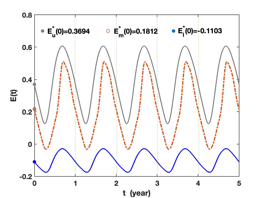
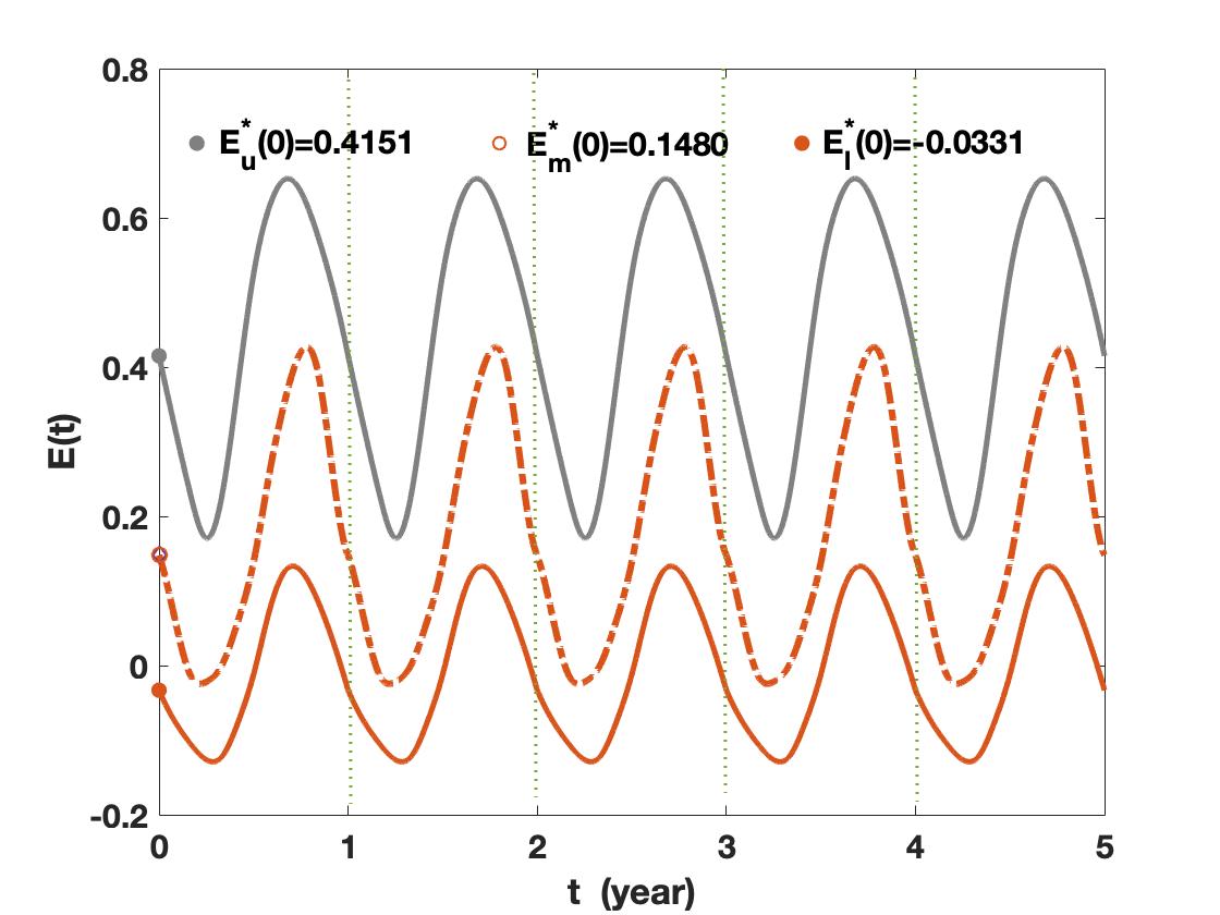
Figure 1: The periodic solutions of the deterministic system $(\ref{e4})$ with different greenhouse gas forcing (a) $\Delta F_{0}=19$ and (b) $\Delta F_{0}=21$. A blue curve indicates the state that is perennially ice-covered ($E<0$ throughout the seasonally cycle). A grey curve indicates the state that is perennially ice-free ($E>0$ throughout the year). A red solid curve indicates the state that is seasonally ice-free ($E<0$ and $E>0$ at different phases in the seasonal cycle). A red dashed curve indicates the state that is an unstable intermediate state in which the Arctic Ocean is partially covered by ice and absorbs just enough solar radiation such that it remains at the freezing temperature: adding a small amount of additional sea ice to this unstable state would lead to less solar absorption, cooling, and a further extended sea-ice cover.

For the deterministic Arctic sea ice model $(\ref{e4})$, Eisenman and WettlauferEisenman and Wettlaufer (2009) have constructed a Poincaré map to obtain the periodic solutions, as shown in Fig. 1. Throughout this paper, the “lower” and “upper” stable periodic solutions of the deterministic system are denoted by $E^{*}_{l},E^{*}_{u}$, respectively, and the “middle” metastable one is denoted by $E^{*}_{m}$. In order to facilitate the numerical calculation, we write the deterministic model using the scale transformation $E/100$.

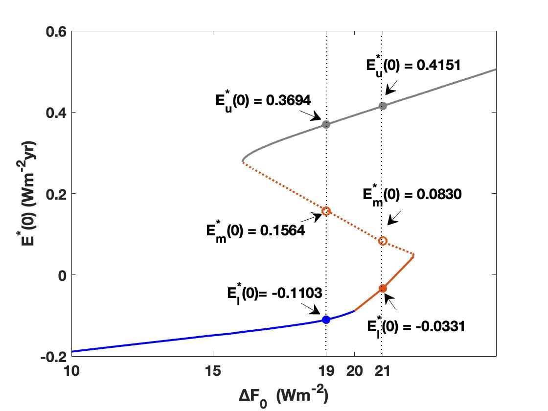
Figure 2: A bifurcation diagram computed from a Poincaré map associated with equation (5). The bifurcation parameter is $\Delta F_{0}$ and the response of the system is represented by $E^{*}(0)$, the energy on 1 January.

In the case of Arctic sea ice, a fixed point corresponds to a steady state solution of the yearly cycle of ice growth and retreat Abbot, Silber, and Pierrehumbert (2011). In this paper we use the method used by Hill, Abbot, and Silber Hill, Abbot, and Silber (2016) to construct Poincaré maps, which indicate the energy changes from 1 January in one year ($E_{n}(0)$) to 1 January in the next year ($E_{n+1}(0)=f(E_{n}(0))$) for a range of initial energies. Fixed points $E^{*}_{n}(0)$ of the Poincaré map occur when $E_{n+1}(0)=f(E^{*}_{n}(0))=E^{*}_{n}(0)$, and they correspond to the periodic solutions of the system with the same periodicity as the forcing (i.e., annual). For different greenhouse gas forcing, $\Delta F_{0}$, we use a Poincaré map to get the fixed points. As shown in Fig. 2, for $\Delta F_{0}\in[10,16)$, there is only one stable fixed point, corresponding to the perennially ice-covered state. For $\Delta F_{0}\in[16,20]$, there are two stable fixed points (the perennially ice-covered state and the perennially ice-free one) and one unstable intermediate fixed point. For $\Delta F_{0}\in(20,23]$, there are two stable fixed points: the seasonally ice-free state and the perennially ice-free state. For $\Delta F_{0}\in(23,25]$, there is only one stable fixed point, which is the perennially ice-free state.

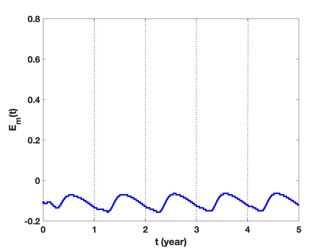
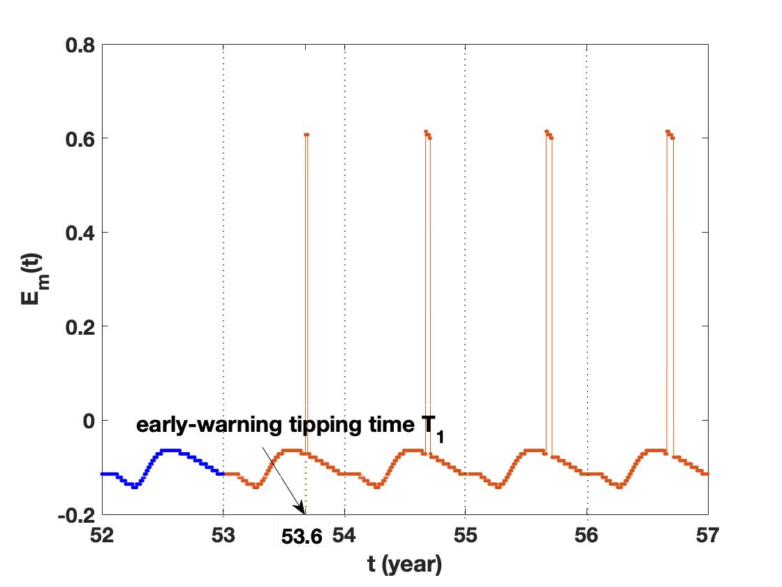
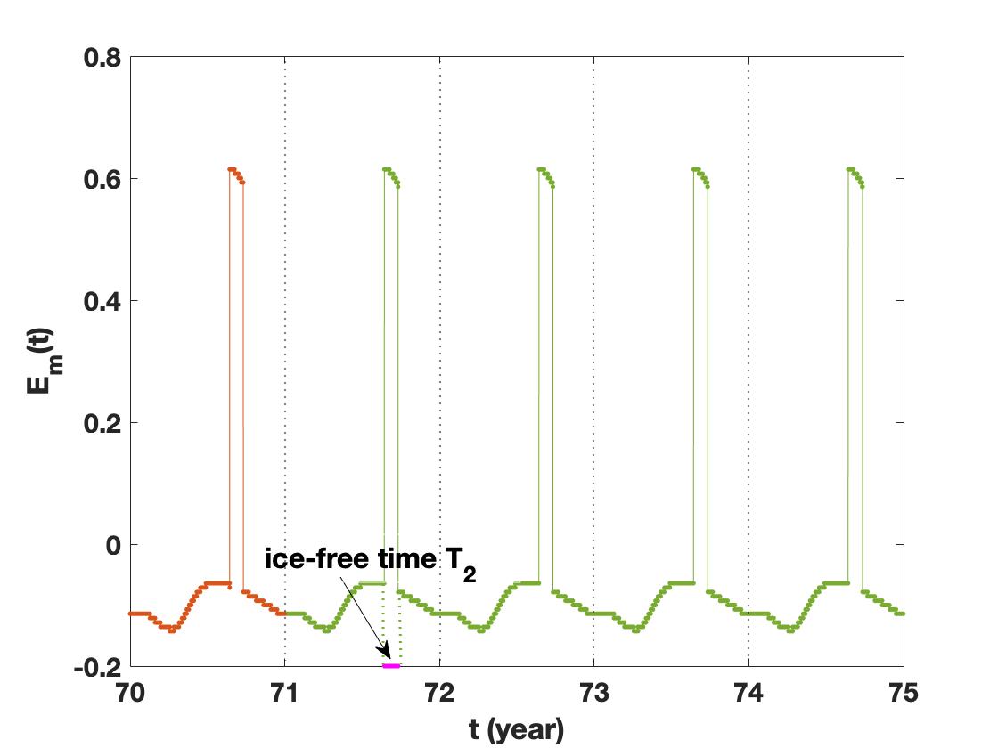
Figure 3: (a) The maximal likely trajectory of the nonautomous SDE $(\ref{e8})$ with the enhanced greenhouse gas level $\Delta F_{0}=19$, Lévy index $\alpha=1.50$ and noise intensity $\epsilon=0.0450$. (b) The enlargement of the blue curve in (a), which shows a perennially ice-covered state ( since $E_{m}<0$ throughout the year). (c) The enlargement of the connection between blue curve and red curve in (a), which displays the transition from the perennially ice-covered state to the seasonally ice-free state. (d) The enlargement of the connection between red curve and green curve in (a), which shows that the system reaches the seasonally ice-free state.

D. Stochastic Arctic sea ice model

The dynamical system $(\ref{e4})$ is a deterministic model. Even though it successfully captures the seasonal cycle of Arctic sea ice thickness and predicts the nature of the transitions as the greenhouse gas forcing $\Delta F_{0}$ increases. However, a realistic feature of the dynamic behavior of the ice cover is its variability due to internal fluctuations and external forcing Fetterer and Untersteiner (1998). Following Ditlevsen Ditlevsen (1999), we consider the following nonautonomous differential equation driven by a scalar symmetric $\alpha$-stable Lévy process with $1\leqslant\alpha\leqslant 2$:

$$dE=f(E,t)dt+\varepsilon dL^{\alpha}_{t},$$ (6)

where the term is $f(E,t)=\left(1-\alpha(E)\right)F_{S}(t)-F_{0}(t)-F_{T}(t)T(t,E)+\Delta F_{0}+F_{B}+\nu_{0}\mathit{R}(-E)$ corresponds to the right side of equation (5). The positive quantity $\varepsilon$ denotes the noise intensity. Thus, equation (6) represents the Arctic sea ice model subject to extreme events as modeled by a non-Gaussian $\alpha$-stable Lévy process. This is a pure jump process when the Lévy index $\alpha$ satisfies $1\leq\alpha<2$. It is known that a pure $\alpha$-stable Lévy process has smaller jumps with higher jump probabilities as $\alpha$ approaches $2$. In this stochastic system, the noise intensity and Lévy index can be regarded as the intensity and the frequency of the extreme events. The special case $\alpha=2$ corresponds to the usual Gaussian process, which is used to model “normal" atmospheric fluctuations.

III Results

In this section, we analyse how the noise intensity $\epsilon$, Lévy index $\alpha$ and greenhouse gas forcing $\Delta F_{0}$ affect the maximal likely trajectory of the nonautonomous SDE $(\ref{e8})$. We determine the tipping times for transitions from the perennially ice-covered state to the seasonally ice-free one, and from the seasonally ice-free state to the perennially ice-free one. In the following, we choose one century (i.e. $T=100$) as the computational terminal time. Computations are carried out over a time interval of one century, that is, $T=100$ years. Following Eisenman and Wetlafer Eisenman and Wettlaufer (2009) we use the terminology “summer” sea ice to refer to the annual minimum of Arctic sea-ice area and thickness and “winter” sea ice to refer to the annual maximum.

A. Effect of $\alpha$-stable Lévy process for the weakened greenhouse effect level $\Delta F_{0}=19$

For the relatively weak greenhouse gas level $\Delta F_{0}=19$, Fig. 3 illustrates the maximal likely trajectory from the perennially ice-covered state to the seasonally ice-free state for Lévy index $\alpha=1.50$ and noise intensity $\epsilon=0.0450$. The blue curve indicates that the stochastic system maintains a perennially ice-covered state, which is enlarged in Fig. 3. The red curve indicates that the system has entered an unstable regime of operation. During the computational time interval of one century, the system begins to experience an ice-free state for a small fraction of time each year. Each year thereafter, the length of time in the fractionally ice-free state increases (see Fig. 3) until the system enters a stable regime of operation in which the length of time in the fractionally ice-free state remains constant, as shown in Fig. 3.

Based on the behavior discussed in the previous paragraph, we refer to the time when the system makes a first transition from a perennially ice-covered state to a state in which a fraction of each year is spent in an ice-free state as the early-warning tipping time, and denote it by $T_{1}$. After $T_{1}$, the ice-covered period is decreasing until the Arctic appears in ice-free state in summer. $T_{1}$ could be regarded as an early-warning signal of anomalous Arctic sea ice, and it helps us to predict the approximate time when Arctic sea ice will disappear in summer. If $T_{1}=100$, the system never appears ice-free and it remains in a perennially ice-covered state during our simulation cycle (one century).

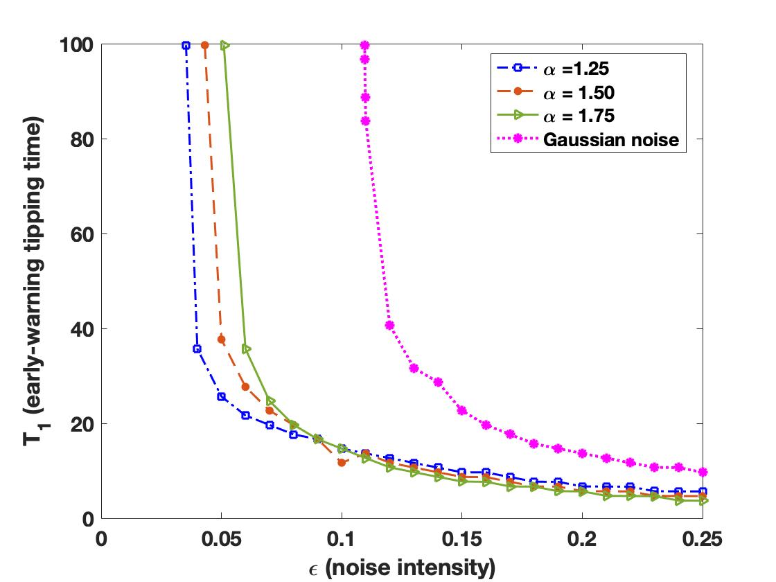
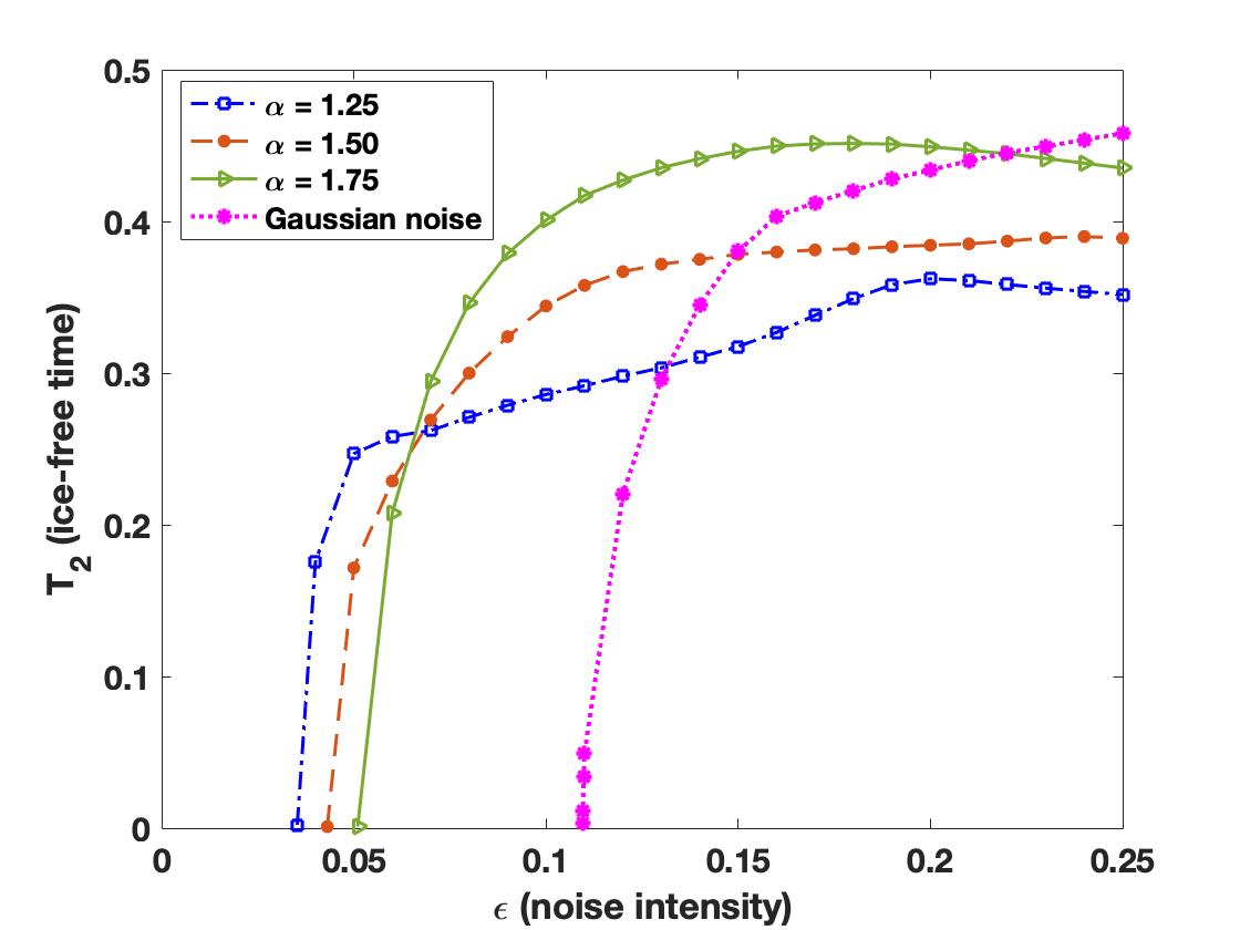
Figure 4: Dependence of (a) the early-warning tipping time $T_{1}$ and (b) the ice-free time $T_{2}$ on the noise intensity $\epsilon$ for $\Delta F_{0}=19$ with non-Gaussian Lévy noise $\alpha=1.25,1.5,1.75$ and Gaussian noise.

We wish to understand the qualitative behavior of the dependence of the early-warning tipping time $T_{1}$ on the Lévy index $\alpha\in[1,2]$ and the noise intensity $\epsilon$. This dependence is shown by the graphs in Fig. 4. We find that $T_{1}$ decreases as $\epsilon$ increases. This agrees with the corresponding result for Gaussian noise. For $\epsilon\in[0.051,0.09]$, $T_{1}$ increases as $\alpha$ increases. However, when $\epsilon$ is greater than $0.09$, $T_{1}$ is insensitive to changes in $\alpha$. To determine the smallest value of $\epsilon$ that leads to a transition away from a perennially ice-covered regime within one century, draw a horizontal line in Fig. 4 at a level slightly below $T_{1}=100$. We see that the minimum noise intensity required for such a transition increases as $\alpha$ increases. For $\alpha=1.25,1.5,1.75$, the minimum values of $\epsilon$ are approximately $0.03528,0.043096,0.051$, respectively. For Gaussian noise, the minimum required noise intensity is clearly much larger.

We know that the $\alpha$-stable Lévy process has smaller jumps with higher jump probabilities for larger values of $\alpha$ ($1\leqslant\alpha<2$). This means that the frequency of extreme events increases when Lévy index $\alpha$ approaches $2$, and the intensity of extreme weather events increases as Lévy noise intensity increases. These results on early-warning tipping times show that increased extreme events intensity lead to the earlier melting of the sea ice. For the small intensity of extreme events, the increased frequency of extreme events has a positive effect on predicting the time for sea ice to melt in summer.

Once the sea ice begin to melt in summer, the system becomes unstable, and with evolution of a fraction of each year, the system will reach the seasonally ice-free state. In order to study the effect of non-Gaussian $\alpha$-stable noise on the time when ice-free state appeared in summer, we will introduce the ice-free time $T_{2}$ to represent the period of the year when the Arctic Ocean is ice-free as shown in Fig. 3. It means that the larger $T_{2}$ is, the longer the a period of time for ice-free state in one year. If the climate becomes warmer further, it will be easier to appear a perennially ice-free state for the Arctic Ocean. It is worth pointing out that the Arctic sea ice system remains in the ice-covered state all year round if the ice-free time $T_{2}=0$.

Fig. 4 demonstrates the dependence of the ice-free time $T_{2}$ on the Lévy index $\alpha\in[1,2)$ and the noise intensity $\epsilon$. We find that $T_{2}$ becomes longer as $\epsilon$ increases under influence of both Gaussian and non-Gaussian Lévy noise. Another observation is that there is an intersection point near $\epsilon=0.065$. When $\epsilon$ is larger thane the intersection point, the ice-free time is longer as the value of $\alpha$ increases. However, the ice-free time $T_{2}$ has opposite behavior when $\epsilon$ is smaller than $\epsilon=0.065$.

These results imply that one has to consider both the value of $\alpha$ and $\epsilon$ when we examine a fraction time of each year in an ice-free state. The ice-free period increases as the intensity of extreme events increases. Meanwhile, we see that the decreasing intensity and frequency of extreme events will be effective in reducing ice free times in summer. These results show the importance for studying extreme weather events.

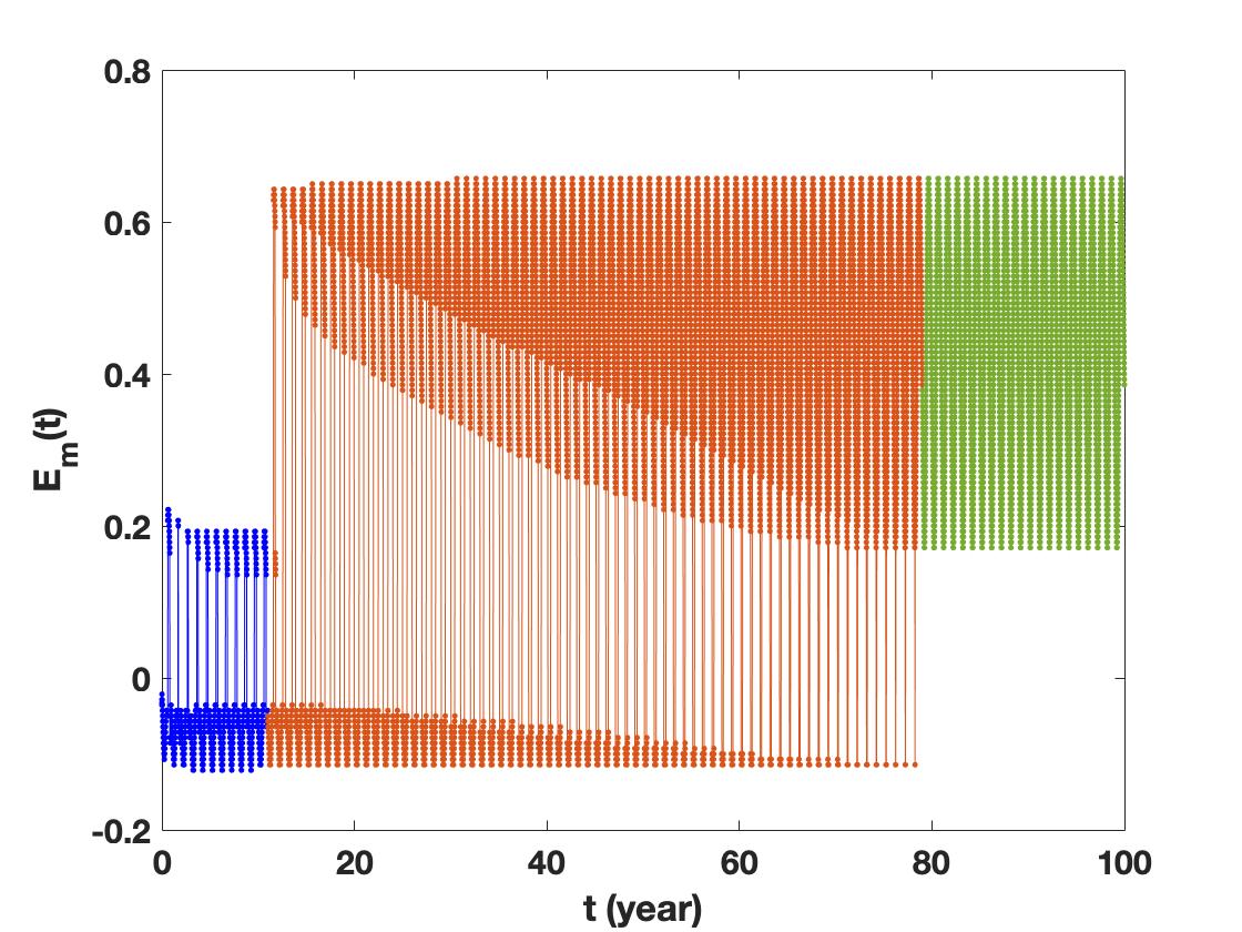
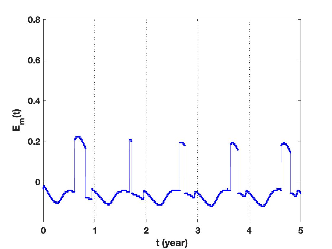
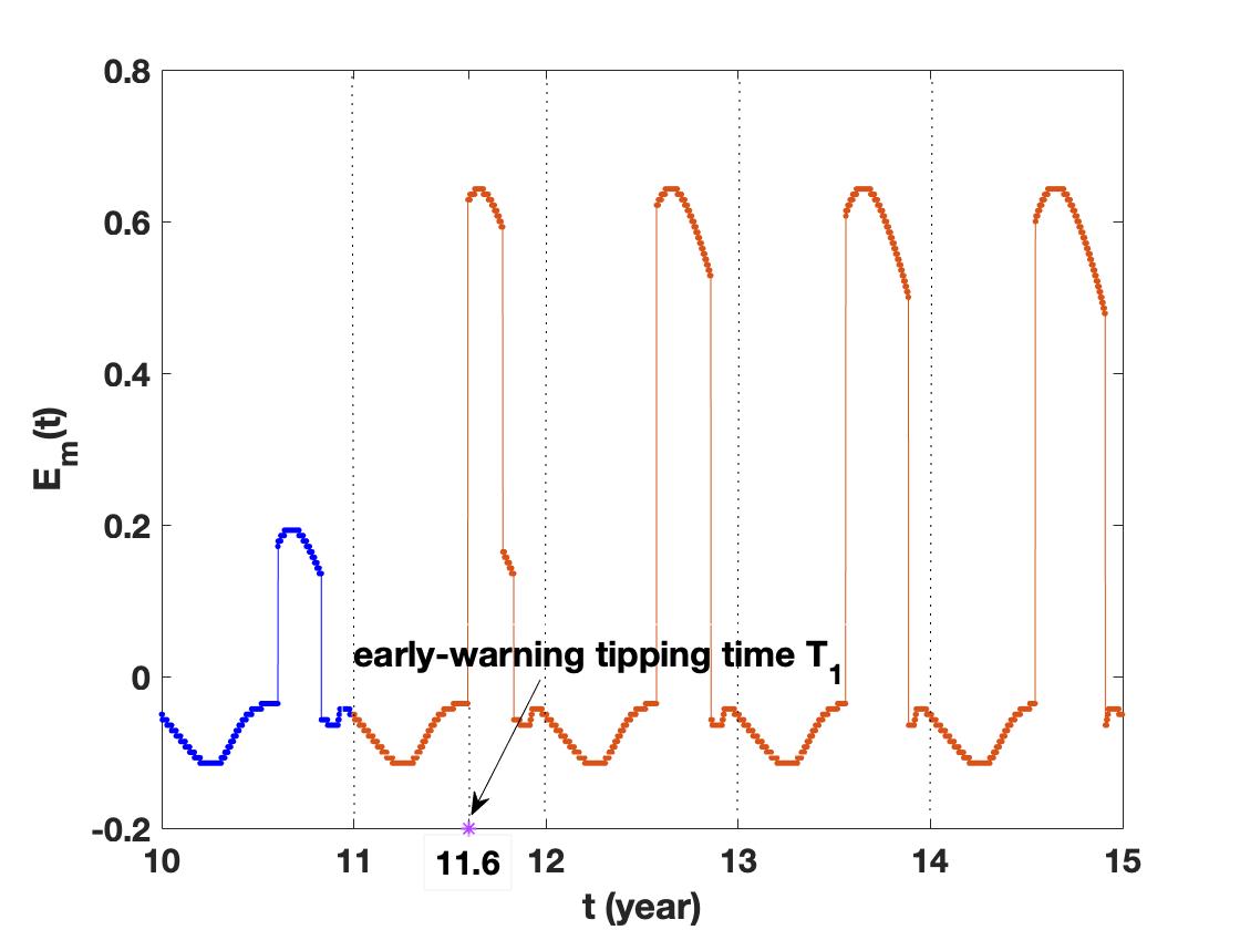
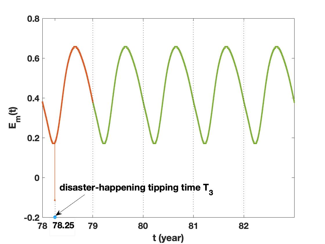
Figure 5: (a) The maximal likely trajectory of the SDE $(\ref{e8})$ with $\Delta F_{0}=21$, Lévy index $\alpha=1.75$ and noise intensity $\epsilon=0.0250$. (b) The enlargement of blue curve in (a), which shows the seasonally ice-free state. (c) The enlargement of the connection between blue curve and red curve in (a), which displays the transition from the seasonally ice-covered state to the perennially ice-free state. (d) The enlargement of the connection between the red curve and the green curve in (a), which shows that the system reaches the perennially ice free state.

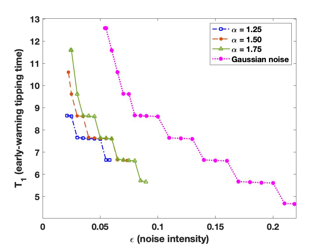
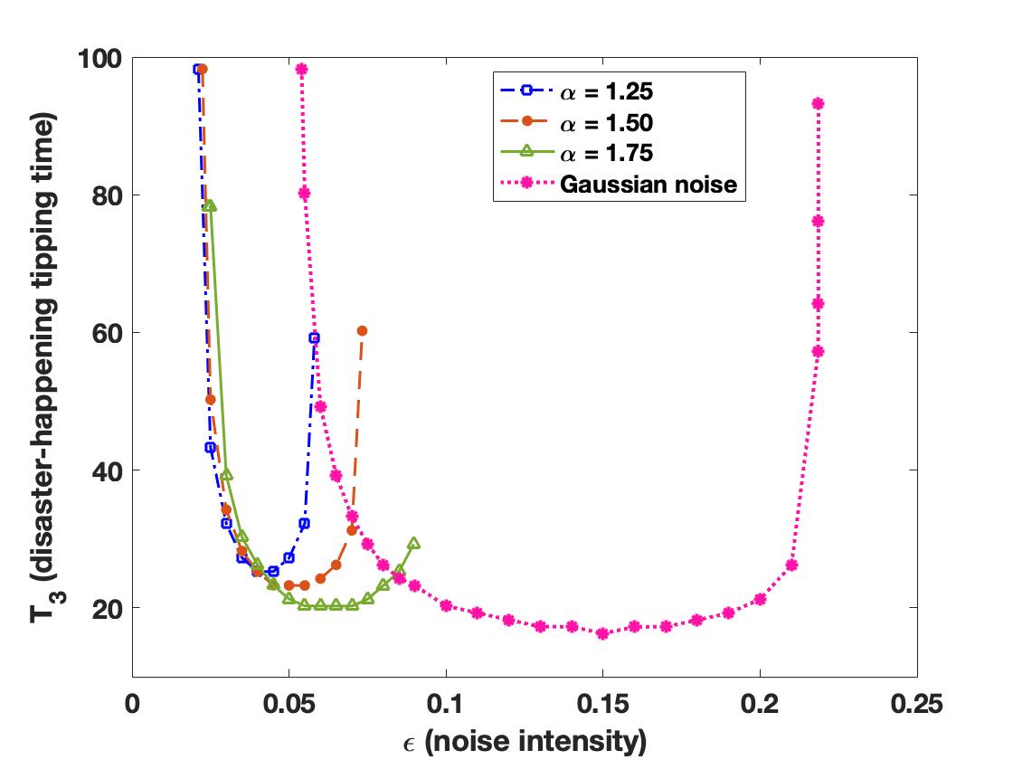
Figure 6: Dependence of (a) the early-warning tipping time $T_{1}$ and (b) the disaster-happening time $T_{3}$ on the noise intensity $\epsilon$ for $\Delta F_{0}=21$ with non-Gaussian Lévy noise $\alpha=1.25,1.5,1.75$ and Gaussian noise.

B. Effect of $\alpha$-stable Lévy process for the enhanced greenhouse effect level $\Delta F_{0}=21$

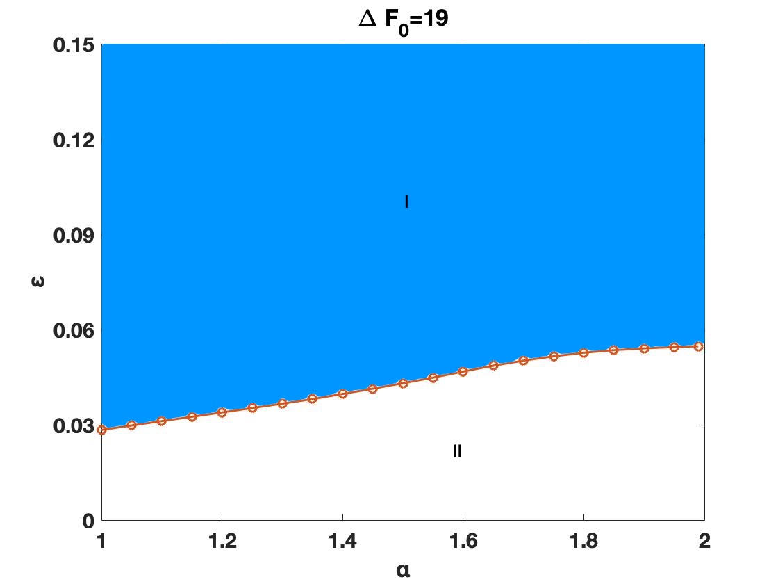
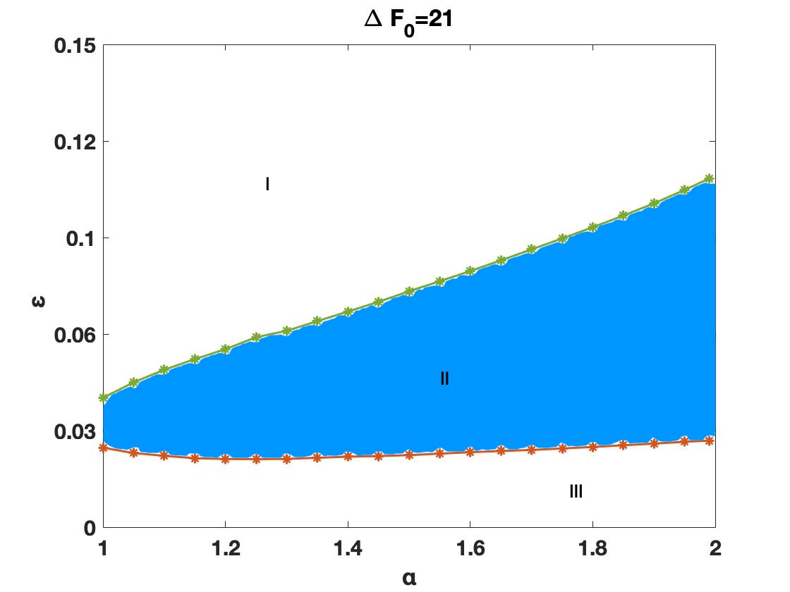
Figure 7: The combination of $\epsilon$ and $\alpha$ which can trigger the transition between metastable states in the Arctic sea ice system. (a) For $\Delta F_{0}=19$, region I: transition from the perennially ice-covered state to the seasonally ice-free one (b) For $\Delta F_{0}=21$, region II: the transition of the Arctic sea ice evolve from the seasonally ice-free state to the perennially ice-free state.

For this larger value of $\Delta F_{0}=21$, the maximal likely trajectory of the nonautonomous SDE $(\ref{e8})$ from the seasonally ice-free state to the perennially ice-free state for Lévy index $\alpha=1.75$ and noise intensity $\epsilon=0.0250$ is shown in Fig. 5. The blue curve represents the stochastic system concentrated on the seasonally ice-free state, as enlarged in Fig. 5. The red curve means that the system has experienced an unstable ice-free state, the length of time in the fractionally ice-free state increases (Fig. 5) until the system remains in a perennially ice-free metastable states (as $E_{m}>0$ throughout the year), as shown in Fig. 5.

To analyze how the system of Arctic sea ice shifts from the seasonally ice-free state to the perennially ice-free state under noise, we will continue to use the early-warning tipping time $T_{1}$ to denote the first time when the seasonally ice-free state changes, as shown in Fig. 5. After $T_{1}$, a fraction of ice-free time increases until the winter sea ice vanishes to the perennially ice-free state. Once this time $T_{1}$ is reached, we should develop and deploy adaptive strategies, and take a more pre-emptive, precautionary policy approach to prevent the situation from getting worse.

Fig. 6 shows that the early-warning tipping time $T_{1}$ presents a ladder descending trend with the increased noise intensity $\epsilon$ for non-Gaussian Lévy noise with $\alpha=1.25,~{}1.50,~{}1.75$. Additionally, for different $\alpha$, we find that the range of Lévy noise intensity that enables the system to shift to the perennially ice-free state is different. For example, for $\alpha=1.25,1.75$, the corresponding transition range of $\epsilon$ is $[0.0211,0.058]$ and $[0.0245,0.0897]$, respectively. On the other hand, for the Gaussian noise, the behaviour of $T_{1}$ agrees in general with the results in previous pure jump case. However, compared with non-Gaussian Lévy noise, Gaussian noise requires the stronger noise intensity and have the larger range of noise intensity for transition to the seasonally ice-free state.

Furthermore, we find that $T_{1}$ obviously appears earlier for the enhanced greenhouse level $\Delta F_{0}=21$ by comparing with the weakened greenhouse level $\Delta F_{0}=19$, as shown in Fig. 6 and 4. For example, keeping $\alpha=1.25$ and $\epsilon=0.04$, the early-warning tipping time close to $35$ and $7$ for $\Delta F_{0}=19$ and $21$, respectively. This means that the Arctic sea ice will melt much earlier under influence of the enhanced greenhouse effect.

For $\Delta F_{0}=21$, the ice-free time $T_{2}\equiv 1$, because the system keep in the perennially ice-free state. In this case, the Arctic Ocean is ice-free all over the year. Therefore, the ice-free time $T_{2}$ can not capture the dynamical behaviour in this case. Next, we will introduce the other quantity, which can help us to predict the approximate time when the thickest ice sheet of the Arctic region in a year will disappear. The disaster-happening tipping time T3 will be introduced to express the last time when the Arctic Ocean has the winter sea ice, and after that time, the Arctic Ocean remains ice-free throughout the year, as shown in Fig. 5. The time $T_{3}$ is a signal of disaster that may happen in Arctic sea ice with unimaginable consequences–from the loss of polar bear habitat to possible increases of weather extremes at mid-latitudes Kerr (2012). We hope that the $T_{3}$ never shows up.

Fig. 6 shows the numerical results of the disaster-happening tipping time $T_{3}$ effect of the noise intensity $\epsilon$ and Lévy index $\alpha=1.25,~{}1.50,~{}1.75$. We find that $T_{3}$ shows a U-shaped changing trend with the increasing of value of $\epsilon$ for the case of non-Gaussian Lévy noise. In the beginning, $T_{3}$ decreases rapidly as $\epsilon$ increases. Then, the effect of the increasing $\epsilon$ on $T_{3}$ is relatively weak. Finally, $T_{3}$ will turn a corner when the curve reaches a nadir, after this inflection point, $T_{3}$ rapidly grows with increasing of $\epsilon$. Furthermore, the value of $\alpha$ is larger, the growth rate of $T_{3}$ is slower. This means that it will delay the time for the appearance of the perennially ice-free state when the intensity of extreme events increases to a certain degree. Meanwhile, the stronger the frequency of extreme events is, the slower the delay time will be. A possible explanation for these inflection points could be the interaction between the ice albedo feedback and the greenhouse effect. We note that for the case of Gaussian noise, relations between the disaster-happening tipping time $T_{3}$ and the value of noise intensity are similar to the non-Gaussian Lévy noise, while the appearance of inflection point requires the stronger noise intensity.

C. Combination of Lévy noise intensity $\epsilon$ and Lévy index $\alpha$ trigger transition

For $\Delta F_{0}=19$ and a fixed value of $\alpha\in[1,2)$, Fig. 7 shows the minimum $\epsilon$ that can trigger transition from the perennially ice-covered state to the seasonally ice-free state, which is marked with red solid points. For example, for $\alpha=1.0,1.75$, the minimum noise intensity that can trigger the transition is $\epsilon\approx 0.03,0.051$, respectively. The larger $\alpha$ is, the larger noise intensity is needed. We collect all the combinations of $\alpha$ and $\epsilon$ that can induce the transitions for Arctic sea ice system in the region I .

Similarly, the combinations of $\alpha$ and $\epsilon$ leading to the transition from the seasonally ice-free state to the perennially ice-free state can be obtained for $\Delta F_{0}=21$, as shown in Fig. 7. For example, for $\alpha=1.5$, the minimum value of noise intensity is $\epsilon\approx 0.02114$ and the maximum value of noise intensity is $\epsilon\approx 0.055$. As shown in Fig. 7, the blue curve and red curve denote an upper bound and a lower bound of $\epsilon$, which correspond to the maximum and minimum noise intensities inducing the transition, respectively. These two curves constitute the region II where the system can shift to a perennially ice-free state from a seasonally ice-free state .

IV Conclusions

Arctic sea ice in recent summers shows the record lows in ice extent Stroeve et al. (2005); Walker (2016). It has also been thinning at a remarkable rate over the past few decades Bitz and Roe (2004); Muller-Stoffels and Wackerbauer (2011). To insight into the Arctic sea ice variations under influence of extreme weather events, we propose a nonautonomous Arctic sea ice model under the non-Gaussian $\alpha$-stable Lévy noise. We use the maximal likely trajectory, based on the numerical solution of the nonlocal Fokker-Planck equation (2), to obtain the tipping times for the stochastic Arctic sea ice model (6). The early-warning tipping time $T_{1}$ and the disaster-happening tipping time $T_{3}$ are used to predict the time when the Arctic Ocean may appear in ice-free state in summer and in winter, respectively.

By numerical experiments, we find that the tipping times $T_{1}$ and $T_{3}$ depend strongly on the Lévy index $\alpha$, noise intensity $\epsilon$ and greenhouse effect $\Delta F_{0}$. For example, for the enhanced greenhouse level $\Delta F_{0}=21$, the early-warning tipping time $T_{1}$ decreases with the increased intensity of $\alpha$-stable Lévy noise, in agreement with the corresponding results for the weakened greenhouse level $\Delta F_{0}=19$, but $T_{1}$ comes earlier for $\delta F_{0}=21$. This implies that Arctic sea ice will melt much earlier in summer under influence of the enhanced greenhouse effect and increased noise intensity. On the other hand, the disaster-happening tipping time $T_{3}$ shows a U-shaped changing trend under non-Gaussian Lévy noise with the increase of value of $\epsilon$. Another observation from the results is that for the ice-free time $T_{2}$, we see that the decreased intensity and frequency of extreme events will be effective in reducing the length of time in the fractionally ice-free state.

Comparing with the non-Gaussian Lévy noise, we discover that a larger noise intensity is needed to induce a transition between metastable states in Gaussian case (see Fig.4 and Fig.6). Finally, we identify the combinations of $\alpha$ and $\epsilon$ that trigger the transitions from one state to the other one in the Arctic sea ice system under non-Gaussian Lévy noise for both the weakened and the enhanced greenhouse gas levels.

Our work provides a theoretical framework for studying and predicting the Arctic sea ice variations under the influence of extreme events.

Appendix A: symmetric $\alpha$-stable Lévy process

It is well known that Brownian motion has the stationary, the independent increments and almost surely continuous sample paths. A Lévy process is a non-Gaussian process with heavy-tailed statistical distribution and intermittent bursts. The stable distribution $S_{\alpha}(\delta,\beta,\lambda)$ is determined by the following four indexes: Lévy index $\alpha\in(0,2)$, scale parameter $\delta\in[0,\infty)$, skewness parameter $\beta\in[-1,1]$ and shift parameter $\lambda\in(-\infty,\infty)$ Duan (2015).

A scalar symmetric $\alpha$-stable Lévy process $L^{\alpha}_{t}$ is defined via the following properties:

• $L^{\alpha}_{0}=0$, almost surely (a.s.);

• $L^{\alpha}_{t}$ has independent increments: For every natural number $n$ and positive time instants with $t_{0}<t_{1}<\cdots<t_{n}$, the random variables $L^{\alpha}_{t_{1}}-L^{\alpha}_{t_{0}}$, $L^{\alpha}_{t_{2}}-L^{\alpha}_{t_{1}}$, $\cdots$, $L^{\alpha}_{t_{n}}-L^{\alpha}_{t_{n-1}}$ are independent;

• $L^{\alpha}_{t}$ has stationary increments: $L^{\alpha}_{t}-L^{\alpha}_{s}$ and $L^{\alpha}_{t-s}$ have the same stable distribution $S_{\alpha}((t-s)^{\frac{1}{\alpha}},0,0)$, for $t>s$;

• $L^{\alpha}_{t}$ has stochastically continuous sample paths: $L^{\alpha}_{t}\rightarrow L^{\alpha}_{s}$ in probability, as $t\rightarrow s$.

An $\alpha$-stable Lévy process $L^{\alpha}$ has the following “heavy tail” estimate Zheng et al. (2020):

$$\lim_{y\rightarrow\infty}y^{\alpha}\mathbb{P}(L^{\alpha}>y)=C_{\alpha}\frac{1+\beta}{2}\sigma^{\alpha},$$

i.e., the tail estimate decays in power law. The constant $C_{\alpha}$ is a gamma function depending on $\alpha$.

For a symmetric $\alpha$-stable Lévy process $L^{\alpha}_{t}$, the skewness index $\beta$ is equal to $0$. The paths of $L^{\alpha}_{t}$ have countable jumps, and the jump measure $\nu_{\alpha}(dy)$ depends on $\alpha$,

$$\nu_{\alpha}(dy)=C_{\alpha}\mid y\mid^{-(1+\alpha)}dy,$$

For $0<\alpha<1$, $L^{\alpha}_{t}$ has larger jumps with lower jump probabilities, while for $1<\alpha<2$, it has smaller jumps with higher jump frequencies. The special case for $\alpha=2$ corresponds to a Brownian motion, and it is a Cauchy process for $\alpha=1$. More information on $\alpha$-stable Lévy process, see references Saltzman (2002); Duan (2015).

Appendix B: Descriptions and Default Values of Model Parameters

Table 1: Descriptions and Default Values of Model Parameters

Symbol	Description	Value
$L_{i}$	Latent heat of fusion of ice	9.5 $Wm^{-3}yr$
$c_{ml}H_{ml}$	Ocean mixed layer heat capacity times depth	$6.3Wm^{-2}yrK^{-1}$
$k_{i}$	Ice thermal conductivity	$2Wm^{-1}K^{-1}$
$F_{B}$	Heat flux into bottom of sea ice or ocean mixed layer	$2Wm^{-2}$
$h_{\alpha}$	Ice thickness range for smooth transition from $\alpha_{i}$ to $\alpha_{ml}$	$0.5m$
$\nu_{0}$	Dynamic export of ice from model domain	$0.1yr^{-1}$
$\alpha_{i}$	Albedo when surface is ice cover	$0.68$
$\alpha_{ml}$	Albedo when ocean mixed layer is exposed	$0.2$
$F_{0}(t)$	Temperature-independent surface flux (seasonally varying)	$85Wm^{-2}$
$F_{T}(t)$	Temperature-dependent surface flux (seasonally varying)	$2.8Wm^{-1}K^{-1}$
$F_{S}(t)$	Incident shortwave radiation flux (seasonally varying)	$100Wm^{-2}$
$\Delta F_{0}$	Imposed surface heat flux	$0Wm^{-2}$

For the seasonally varying parameters $F_{0}(t)$, $F_{T}(t)$ and $F_{S}(t)$, the monthly values starting with January are $F_{0}(t)$=(120, 120, 130, 94, 64, 61, 57, 54, 56, 64, 82, 110) $Wm^{-2}$, $F_{T}(t)$=(3.1, 3.2, 3.3, 2.9, 2.6, 2.6, 2.6, 2.5, 2.5, 2.6, 2.7, 3.1)$Wm^{-2}K^{-1}$, and $F_{S}(t)$=(0, 0, 30, 160, 280, 310, 220, 140, 59, 6.4, 0, 0)$Wm^{-2}$.

Data Availability Statement

The data that support the findings of this study are openly available on GitHub Yang (2020).

References

- Min et al. (2008) S. Min, X. Zhang, F. W. Francis, and T. Agnew, “Human influence on arctic sea ice detectable from early 1990s onwards,” Geophysical Research Letters 35 (2008).
- Notz and Marotzke (2012) D. Notz and J. Marotzke, “Observations reveal external driver for arctic sea-ice retreat,” Geophysical Research Letters 39 (2012).
- Scheweiger, Wood, and Zhang (2019) A. J. Scheweiger, K. R. Wood, and J. Zhang, “Arctic sea ice volume variability over 1901–2010: A model-based reconstruction.” Journal of Climate 32, 4731–4752 (2019).
- Budyko (1969) M. I. Budyko, “The effect of solar radiation variations on the climate of the earth,” Tellus 21, 611–619 (1969).
- Sellers (1969) W. D. Sellers, “A global climate model based on the energy balance of the earth-atmosphere system,” Journal of Applied Meteorology 8, 392–400 (1969).
- North, Gahalan, and Jr (1981) G. R. North, R. F. Gahalan, and J. A. C. Jr, “Energy balance climate models,” Reviews of Geophysics 19, 91–121 (1981).
- Crowley (2000) T. J. Crowley, “Causes of climate change over the past 1000 years,” Science 289, 270–277 (2000).
- Zhang, Rothrock, and Steele (2000) J. Zhang, D. Rothrock, and M. Steele, “Recent changes in arctic sea ice: The interplay between ice dynamics and thermodynamics,” Journal of Climate 13, 3099–3114 (2000).
- Moon and Wettlaufer (2017) W. Moon and J. S. Wettlaufer, “A stochastic dynamical model of arctic sea ice,” Journal of Climate 30, 5119–5140 (2017).
- Eisenman and Wettlaufer (2009) I. Eisenman and J. S. Wettlaufer, “Nonlinear threshold behavior during the loss of arctic sea ice,” PNAS 106, 28–32 (2009).
- Abbot, Silber, and Pierrehumbert (2011) D. S. Abbot, M. Silber, and R. T. Pierrehumbert, “Bifurcations leading to summer arctic sea ice loss,” Journal of Geophysical Research-Atmospheres 116 (2011).
- Hill, Abbot, and Silber (2016) K. Hill, D. S. Abbot, and M. Silber, “Analysis of an arctic sea ice loss model in the limit of a discontinuous albedo,” SIAM Journal on Applied Dynamical Systems 15, 1163–1192 (2016).
- Gao et al. (2016) T. Gao, J. Duan, X. Kan, and Z. Cheng, “Dynamical inference for transitions in stochastic systems with -stable levy noise,” Journal of Physics A: Mathematical and Theoretical 49, 294002 (2016).
- Kampen (1976) N. G. V. Kampen, “Stochastic differential equation,” Physics Reports 24, 171–228 (1976).
- Hasselman (1976) K. Hasselman, “Stochastic climate models. Part I. Theory,” Tellus 28, 473–485 (1976).
- Agarwal and Wettlaufer (2018) S. Agarwal and J. S. Wettlaufer, “Fluctuations in arctic sea ice extent: comparing observations and climate models,” Philosophical Transactions of Royal Society A: Mathematical, Physical and Engneering Sciences 376 (2018).
- Chen et al. (2019) Y. Chen, J. A. Gemmer, M. Silber, and A. Volkening, “Noise-induced tipping under periodic forcing: Preferred tipping phase in a non-adiabatic forcing regime,” Chaos 29, 043119 (2019).
- Farazmand and Sapsis (2017) M. Farazmand and T. P. Sapsis, “A variational approach to probing extreme events in turbulent dynamical systems,” Science Advances 3, e1701533 (2017).
- Selmi et al. (2016) F. Selmi, S. Coulibaly, Z. Loghmari, I. Sagnes, G. Beaudoin, M. G. Clerc, and S. Barbay, “Spatiotemporal chaos induces extreme events in an extended microcavity laser,” Physical Review Letters 116, 013901 (2016).
- Ditlevsen (1999) P. D. Ditlevsen, “Observation of -stable noise induced millennial climate changes from an ice-core record,” Geophysical Research Letters 26, 1441–1444 (1999).
- Zheng et al. (2020) Y. Zheng, F. Yang, J. Duan, X. Sun, L. Fu, and J. Kurths, “The maximum likelihood climate change for global warming under the influence of greenhouse effect and lévy noise,” Chaos 30, 013132 (2020).
- Livina and Lenton (2013) V. Livina and T. M. Lenton, “A recent tipping point in the arctic sea-ice cover: abrupt and persistent increase in the seasonal cycle since 2007,” Cryosphere 7, 275–286 (2013).
- Lenton et al. (2008) T. M. Lenton, H. Held, E. Kriegle, J. W. Hall, W. Lucht, S. Rahmstor, and H. J. Schellnhuber, “Tipping elements in the earth’s climate system,” PNAS 105, 1786–1793 (2008).
- Ashwin et al. (2012) P. Ashwin, S. Wieczorek, R. Vitolo, and P. Cox, “Tipping points in open systems: bifurcation, noise-induced and rate-independent examples in the climate system.” Philosophical Transactions of the Royal Society A: Mathemathical,Physical and Engineering Sciences 370, 1166–1184 (2012).
- Sutera (1981) A. Sutera, “On stochastic perturbation and long-term climate behaviour,” Quarterly Journal of the Royal Meteorological Society 107, 137–151 (1981).
- Lucarini and Bódai (2017) V. Lucarini and T. Bódai, “Edge states in the climate system: exploring global instabilities and critical transitions,” Nonlinearity 30, R32–R66 (2017).
- Lucarini and Bódai (2019) V. Lucarini and T. Bódai, “Transitions accross melancholia states in a climate model: Reconciling the deterministic and stochastic points of view,” Physical Review Letters 122, 158701 (2019).
- Duan (2015) J. Duan, An Introduction to Stochastic Dynamics (Cambridge University Press, 2015).
- Sun and Duan (2012) X. Sun and J. Duan, “Fokker-Planck equations for nonlinear dynamical systems driven by non-Gaussian Lévy processes,” Journal of Mathematical Physics 53, 072701 (2012).
- Gao, Duan, and Li (2016) T. Gao, J. Duan, and X. Li, “Fokker-Planck equations for stochastic dynamical systems with symmetric Lévy motions,” Applied Mathematics and Computation 278, 1–20 (2016).
- Zeitouni and Dembo (1987) O. Zeitouni and A. Dembo, “A maximum a posteriori estimator for trajectories of diffusion processes,” Stochastics 20, 221–246 (1987).
- Zeitouni and Dembo (1988) O. Zeitouni and A. Dembo, “An existence theorem and some properties of maximum a posteriori estimators of trajectories of diffusions,” Stochastics 23, 197–218 (1988).
- Maykut and Untersteiner (1971) G. A. Maykut and N. Untersteiner, “Some results from a time-dependent thermodynamic model of sea ice,” Journal of Geophysical Research 76, 1550–1575 (1971).
- Fetterer and Untersteiner (1998) F. Fetterer and N. Untersteiner, “Observations of melt ponds on arctic sea ice,” Journal of Geophysical Research-Oceans 103, 24821–24835 (1998).
- Kerr (2012) R. A. Kerr, “Ice-free arctic sea may be years, not decades, away,” Science 337, 1591–1591 (2012).
- Stroeve et al. (2005) J. C. Stroeve, M. C. Serreze, F. Fetterer, T. Arbetter, W. Meier, J. Maslanik, and K. Knowles, “Tracking the arctic’s shriking ice cover: Another extreme september minimum in 2004,” Geophysical Research Letters 32 (2005).
- Walker (2016) G. Walker, “The tipping point of the iceberg,” Nature 441, 802–805 (2016).
- Bitz and Roe (2004) C. M. Bitz and G. H. Roe, “A mechanism for the high rate of sea ice thinning in the arctic ocean,” Journal of Climate 17, 3623–3632 (2004).
- Muller-Stoffels and Wackerbauer (2011) M. Muller-Stoffels and R. Wackerbauer, “Regular network model for the sea ice-albedo feedback in the arctic,” Chaos 21 (2011).
- Saltzman (2002) B. Saltzman, Dynamical Paleoclimatology (Academic Press, 2002).
- Yang (2020) F. Yang, “Code,” Github (2020), https://github.com/yangfang0914/The-tipping-times-in-an-arctic-sea-ice-system-under-influence-of-extreme-events.