Lifshitz Transition in Triangular Lattice Kondo-Heisenberg Model

Abstract

Motivated by recent experimental progress on triangular lattice heavy-fermion compounds, we investigate possible Lifshitz transitions and the scanning tunnel microscope (STM) spectra of the Kondo-Heisenberg model on the triangular lattice. In the heavy Fermi liquid state, the introduced Heisenberg antiferromagnetic interaction ($J_{H}$) results in the twice Lifshitz transition at the case of the nearest-neighbour electron hopping but with next-nearest-neighbour hole hopping and the case of the nearest-neighbour hole hopping but with next-nearest-neighbour electron hopping, respectively. Driven by $J_{H}$, the Lifshitz transitions on triangular lattice are all continuous in contrast to the case in square lattice. Furthermore, the STM spectra shows rich line-shape which is influenced by the Kondo coupling $J_{K}$, $J_{H}$ and the ratio of the tunneling amplitude $t_{f}$ versus $t_{c}$. Our work provides a possible scenario to understand the Fermi surface topology and the quantum critical point in heavy-fermion compounds.

I Introduction

The Lifshitz transition, where the Fermi surface (FS) topology changes,lifshitz1960 is beyond the paradigm of Landau’s symmetry breaking theory. This unconventional transition has been observed experimentally in cuprate superconductors,PhysRevB.81.180513 ; PhysRevLett.114.147001 ; PhysRevB.83.054506 iron-based superconductors,PhysRevLett.112.156401 ; PhysRevB.89.224517 ; cho2016energy ; PhysRevB.90.224508 ; PhysRevLett.103.047002 ; PhysRevB.83.020501 ; PhysRevB.86.165117 ; PhysRevB.88.220508 ; liu2010evidence topological insulator,volovik2017topological graphenePhysRevB.96.155432 and heavy-fermion compounds.PhysRevLett.96.026401 ; PhysRevLett.99.056401 ; PhysRevB.79.214428 ; PhysRevB.83.115133 ; PhysRevLett.110.256403 ; PhysRevLett.116.037202 Particularly, for some quantum critical heavy-fermion materials, such as YbRh₂Si₂, its magnetic field dependent thermopower, thermal conductivity, resistivity and Hall effect shows three transitions at high fields and the Lifshitz transitions are argued to be their origin.PhysRevLett.110.256403 For CeRu₂Si₂, the high resolution Hall effect and magnetoresistance measurements across the metamagnetic transition are explained as an abrupt $f$-electron localization, where one of the spin-split sheets of the heaviest Fermi surface shrink to a point.PhysRevLett.96.026401 The Lifshitz transition leads to the way to understand the relation of the FS topology and the quantum critical point in heavy-fermion systems.paschen2004

Theoretically, the Lifshitz transition in heavy fermion systems have been carefully explored with mean-field theory and dynamical mean-field theory. PhysRevB.83.033102 ; zhong2015fermionology ; LIU2014 ; PhysRevB.86.075108 ; PhysRevB.94.155103 ; PhysRevLett.110.226403 ; PhysRevB.98.045105 ; PhysRevLett.45.1028 ; PhysRevB.61.3435 ; PhysRevLett.110.026403 ; PhysRevLett.111.026401 ; PhysRevB.87.205144 At the mean-field level, the Lifshitz transition is triggered with the introduction of Heisenberg coupling into the usual Kondo lattice model, i.e. Kondo-Heisenberg model (KHM), and a case studying on square lattice suggests both first and second-order Lifshitz transitions.PhysRevB.83.033102 ; zhong2015fermionology ; LIU2014 Interestingly, the appearance of Lifshitz transition with enhanced antiferromagnetic Heisenberg interaction preempts the disentanglement of Kondo singlet, thus the resulting Kondo breakdown mechanism predicted in literature should be reexamined.PhysRevB.86.075108 ; PhysRevB.77.134439 ; PhysRevLett.106.137002

Recently, non-Fermi liquid behaviors have been observed in triangular lattice heavy-fermion compounds like YbAgGe and YbAl₃C₃.PhysRevB.71.054408 ; PhysRevLett.110.176402 ; PhysRevB.69.014415 ; PhysRevLett.111.116401 ; PhysRevB.87.220406 ; PhysRevB.85.144416 Due to the frustration effect introduced by local $f$-electron spin located on the triangular lattice, the observed non-Fermi liquid phenomena could be linked to the idea of Kondo breakdown, where critical Kondo boson and deconfined gauge field induce singularity in thermodynamics and transport.PhysRevB.71.054408 ; PhysRevB.69.014415 ; PhysRevB.85.144416 However, as exemplified by the study on the square lattice, the topology of FS may change radically before any noticeable breakdown of Kondo effect, therefore the possibility of Lifshitz transition on triangular lattice should be investigated firstly.

In the present work, we employ the large-$N$ mean-field approach to study the KHM on the triangular lattice. As expected, we find that the Heisenberg antiferromagnetic interaction ($J_{H}$) induces twice FS topology change at the case of the nearest-neighbour (NN) electron hopping but with next-nearest-neighbour (NNN) hole hopping and the case of the NN hole hopping but with NNN electron hopping. Both Lifshitz transitions are continuous, which is different from the square lattice case, i.e. the first-order and the second-order phase transition.PhysRevB.83.033102 The density of state (DOS) of conduction electron is changed by $J_{H}$. To meet with experiments, we give the STM line-shape of the differential conductance $dI/dV$ for different Kondo coupling ($J_{K}$) and the ratio of the tunneling amplitude of $f$-electron $t_{f}$ versus conduction electron’s $t_{c}$. The calculated spectra are qualitatively consistent with data in CeCoIn₅.aynajian2012visualizing

The paper is organized as follows. In Sec. 2, we describe the Kondo-Heisenberg model under the large-N mean-field theory. In Sec. 3, we present the Lifshitz transition and the DOS of conduction electron. In Sec. 4, we give the line-shape of differential conductance at different Heisenberg antiferromagnetic interaction, the Kondo coupling and the ratio of the tunneling amplitude of f-electron to conduction electron’s. Finally, Sec. 5 is devoted to a brief conclusion and perspective.

II Model and mean-field approach

The model Hamiltonian of the KHM is given by

$$H =-t\sum_{<ij>\sigma}c^{{\dagger}}_{i\sigma}c_{j\sigma}+t_{1}\sum_{\ll ij\gg\sigma}c^{{\dagger}}_{i\sigma}c_{j\sigma}-\mu\sum_{i\sigma}c^{{\dagger}}_{i\sigma}c_{i\sigma}$$ (1)

$$\quad+J_{K}\sum_{i}\textbf{S}_{i}\cdot\textbf{s}_{i}+J_{H}\sum_{<ij>}\textbf{S}_{i}\cdot\textbf{S}_{j},$$

where $c^{{\dagger}}_{i\sigma}(c_{i\sigma})$ denotes the creation (annihilation) operator of conduction electron with spin $\sigma=\uparrow,\downarrow$. The first line in Eq. (1) describes the hoppings of conduction electron and $\mu$ is the chemical potential. $\langle\cdot\rangle$ and $\langle\langle\cdot\rangle\rangle$ represent the NN and the NNN hopping, respectively. (The NNN hopping is introduced to avoid the occasional nesting.) The $J_{K}$ term in the second line denotes the Kondo coupling between the localized $f$-electron and conduction electron. $\textbf{S}_{i}=\frac{1}{2}\sum_{\alpha\beta}f_{i\alpha}^{{\dagger}}\tau_{\alpha\beta}f_{i\beta}$ is the fermionic representation of localized $f$-electron spin with the local constraint $\sum_{\sigma}f^{{\dagger}}_{i\sigma}f_{i\sigma}=1$, while $\textbf{s}_{i}=\frac{1}{2}\sum_{\sigma\sigma^{\prime}}c^{{\dagger}}_{i,\sigma}\tau_{\sigma\sigma^{\prime}}c_{i,\sigma^{\prime}}$ is for conduction electron. The last $J_{H}$ term is the Heisenberg exchange interaction firstly introduced by Coleman and Andrei.Coleman1989 It has also been used by Iglesias et al. to consider the antiferromagnetic long-range order in some Ce-based heavy fermion compounds.Arispe1995255 ; Iglesias1996160 ; Lacroix1997503

To proceed, we use the fermionic large-$N$ mean-field method,Read1983 which is believed to capture qualitative features in heavy Fermi liquid states. Introducing valence-bond order parameter $\chi_{ij}=-\left\langle\Sigma_{\alpha}f^{{\dagger}}_{i\alpha}f_{j\alpha}\right\rangle$ and Kondo hybridization parameter $V=\left\langle\Sigma_{\alpha}f^{{\dagger}}_{i,\alpha}c_{i\alpha}\right\rangle$,PhysRevB.83.033102 and considering the uniform resonance-valence-bond ansatz $\chi_{ij}=\chi$ in Refs. PhysRevB.83.033102 ; Liu2012 , one can obtain $\textbf{S}_{i}\cdot\textbf{S}_{j}=\frac{1}{2}\left[\chi(f^{{\dagger}}_{i\uparrow}f_{j\uparrow}+f^{{\dagger}}_{i\downarrow}f_{j\downarrow})+H.c.\right]+\frac{\chi^{2}}{2}$. Based on these mean-field formulations, Eq.(1) can be rewritten in the $k$-space as follows

$$H=\sum_{k}\Psi^{{\dagger}}_{k}\left(\begin{array}[]{ccc}\varepsilon_{k}-\mu&-\frac{J_{K}V}{2}\\ \\ -\frac{J_{K}V}{2}&\chi_{k}\\ \end{array}\right)\Psi_{k}+\sum_{k\sigma}\chi_{k}f^{{\dagger}}_{k\sigma}f_{k\sigma}$$ (5)

$$\qquad+N_{S}\left(\frac{J_{K}V^{2}}{2}+\frac{3J_{H}\chi^{2}}{2}-\lambda\right),$$ (6)

where $\Psi^{{\dagger}}_{\textbf{k}}=\left(c^{{\dagger}}_{\textbf{k}\sigma},f^{{\dagger}}_{\textbf{k}\sigma}\right)$ is a two-component Nambu spinor, and $\gamma_{k}=2\cos(\sqrt{3}k_{y}/2)\cos(k_{x}/2)+\cos(k_{x})$, $\chi_{k}=J_{H}\chi\gamma_{k}+\lambda$ is the kinetic energy of the $f$-electron, and $\varepsilon_{k}=2t_{1}[2\cos(\sqrt{3}k_{y}/2)\cos(3k_{x}/2)+\cos(\sqrt{3}k_{y})]-2t\gamma_{k}$ denoting the energy spectrum of conduction electron. Also, the Lagrangian multiplier $\lambda$ is introduced to impose the local constraint on average. The quasiparticle excitation spectrum can be easily obtained by

$$E^{\pm}_{k}=\frac{(\varepsilon_{k}-\mu+\chi_{k})}{2}\pm\frac{\sqrt{(\varepsilon_{k}-\mu-\chi_{k})^{2}+J^{2}_{K}V^{2}}}{2}.$$ (7)

The ground-state energy of the KHM is

$$E_{g}=\frac{2}{N_{S}}\sum_{k,\pm}E^{\pm}_{k}\theta(-E^{\pm}_{k})+\left(\frac{J_{K}V^{2}}{2}+\frac{3J_{H}\chi^{2}}{2}-\lambda\right),$$ (8)

where $\theta(x)$ is the step function. The factor $2$ comes from the spin degeneracy. Then, the MF equations for $\chi,V,\lambda$ can be derived by minimizing the ground-state energy and the chemical potential $\mu$ is determined by the conduction electron density $n_{c}$, i.e. $\frac{\partial{E_{g}}}{\partial{\chi}}=0,\frac{\partial{E_{g}}}{\partial{V}}=0,\frac{\partial{E_{g}}}{\partial{\lambda}}=0,-\frac{\partial{E_{g}}}{\partial{\mu}}=n_{c}$. One can get four self-consistent MF equations:

$$-\frac{1}{N_{S}}\sum_{k,\pm}\theta(-E^{\pm}_{k})\gamma_{k}\left[1\mp\frac{(\varepsilon_{k}-\mu-\chi_{k})}{W_{k}}\right]=3\chi,$$ (9)

$$-\frac{1}{N_{S}}\sum_{k,\pm}\theta(-E^{\pm}_{k})\left[\frac{\pm J_{K}}{W_{k}}\right]=1,$$ (10)

$$\frac{1}{N_{S}}\sum_{k,\pm}\theta(-E^{\pm}_{k})\left[1\mp\frac{(\varepsilon_{k}-\mu-\chi_{k})}{W_{k}}\right]=1,$$ (11)

$$\frac{1}{N_{S}}\sum_{k,\pm}\theta(-E^{\pm}_{k})\left[1\pm\frac{(\varepsilon_{k}-\mu-\chi_{k})}{W_{k}}\right]=n_{c},$$ (12)

where $W_{k}=\sqrt{(\varepsilon_{k}-\mu-\chi_{k})^{2}+(J_{K}V)^{2}}$.

III Lifshitz transition

We consider the case of $J_{H}\ll J_{K}$, where the paramagnetic heavy Fermi liquid state is stable to other symmetry-breaking and exotic fractionalized states. When the Heisenberg interaction $J_{H}$ increases, the band structure of quasiparticle evolves and Lifshitz transition is expected to occur.

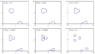
Figure 1: The FS evolution of the KHM versus the Heisenberg interaction $J_{H}$ for NN electron hopping but with NNN hole hopping, where $t=1,t_{1}/t=0.3,n_{c}=0.9,J_{K}=2.5$.

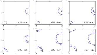
Figure 2: The FS evolution of the KHM versus the Heisenberg interaction $J_{H}$ for NN hole hopping but with NNN electron hopping, where $t=-1,t_{1}/t=0.3,n_{c}=0.9,J_{K}=2.5$.

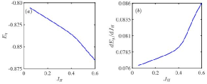
Figure 3: The ground-state energy $E_{g}$ (subplot (a)) and the first derivative $dE_{g}/dJ_{H}$ (subplot (b)) versus the Heisenberg interaction $J_{H}$ for NN electron hopping but with NNN hole hopping, where $t=1,t_{1}/t=0.3,n_{c}=0.9,J_{K}=2.5$.

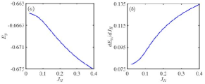
Figure 4: The ground-state energy $E_{g}$ (subplot (a)) and the first derivative $dE_{g}/dJ_{H}$ (subplot (b)) versus the Heisenberg interaction $J_{H}$ for NN hole hopping but with NNN electron hopping, where $t=-1,t_{1}/t=0.3,n_{c}=0.9,J_{K}=2.5$.

In Fig. 1 and Fig. 2, the FS is a normal circle when $J_{H}$ is small as shown in Fig. 1 (a) and Fig. 2 (a), which means the influence of the short-range antiferromagntic correlation is negligible. However, when $J_{H}$ is increasing, the short-range antiferromagnetic correlation starts to change the electronic structure, and the FS begins to deform. Our system have twice Lifshitz transition in two cases as shown in Fig. 1 (d), (e), and Fig. 2 (b), (e). In Fig. 1 (d) and Fig. 2 (b), there emerges a small circle below FS at the center, the particles begin to fill the area between two loops. In Fig. 1 (e) and Fig. 2 (e), the FS happens to split into many Fermi pockets after this critical point, each pocket is the FS of electrons, and they will be shifted inward along the direction M $\rightarrow$ $\Gamma$ associated with $J_{H}$, such as Fig. 1 (f) and Fig. 2 (f). The quantum critical points for NN electron hopping with NNN hole hopping has the larger Heisenberg coupling $J_{H}$ than the case of the NN hole hopping with NNN electron hopping.

Due to many experiments on heavy-fermion quantum critical compounds YbRh₂Si₂ and CeRu₂Si₂,PhysRevLett.110.256403 ; PhysRevLett.96.026401 the FS change relates to the quantum phase transition. Thus, to identify the quantum phase transition around the Lifshitz transition, the ground-state energy $E_{g}$ and its first derivative $dE_{g}/dJ_{H}$ versus $J_{H}$ is shown in Fig. 3 and Fig. 4, where $dE_{g}/dJ_{H}$ is given by

$$\frac{dE_{g}}{dJ_{H}}=\frac{1}{N_{S}}\sum_{k,\pm}\theta(-E^{\pm}_{k})\chi\gamma_{k}\left[1\mp\frac{(\varepsilon_{k}-\mu-\chi_{k})}{W_{k}}\right]+\frac{3\chi^{2}}{2}.$$ (13)

Both lines are smooth across the changes of FS topology, which demonstrates that the Lifshitz transitions are second-order transitions.

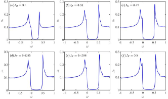
Figure 5: The conduction electron DOS $\rho_{c}$ for the KHM versus the Heisenberg interaction $J_{H}$ for NN electron hopping but with NNN hole hopping, where $t=1,t_{1}/t=0.3,n_{c}=0.9,J_{K}=2.5$. It is shown that the conduction electron DOS is changed after Lifshitz transition.

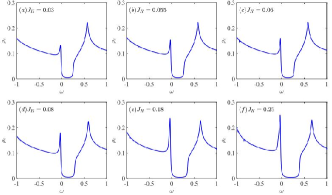
Figure 6: The DOS of the conduction electron $\rho_{c}$ for the KHM versus the Heisenberg interaction $J_{H}$ for NN hole hopping but with NNN electron hopping, where $t=-1,t_{1}/t=0.3,n_{c}=0.9,J_{K}=2.5$. It is shown that the conduction electron DOS is changed after Lifshitz transition.

The DOS of the conduction electron is shown in Figs. 5 - 6. The Heisenberg interaction $J_{H}$ has an effect on the DOS of the conduction electron $\rho_{c}$, the larger $J_{H}$ induces the larger gap. Thus, the DOS is changed after Lifshitz transition. In Fig. 5 (a)-(b), the DOS has a gap and two peaks. At $J_{H}=0.4255$, it develops a new small peak as sown in Fig. 5 (c), where the conduction electron DOS has one gap and three peaks when $J_{H}>0.4255$ as shown in Fig. 5 (c)-(f). In Fig. 6, the DOS always has the gap and two peaks, but the left peak is lower than the right peak as shown in Fig. 6 (a)-(d), while becomes higher than the right peak as shown in Fig. 6 (e)-(f). Both peaks are increasing versus the Heisenberg coupling $J_{H}$, and the peak at $\omega<0$ that arises from the van Hove singularity of the large (hybridized) FS.Figgins2010

Therefore, under the MF method,Liu2012 ; PhysRevB.83.033102 when Heisenberg superexchange $J_{H}$ increases, the presence of the short-range antiferromagnetic correlation gradually changes the electronic structure, and leads to the mentioned two kinds of Lifshitz transition, which is similar to Ref. PhysRevB.83.033102 . However, our work finds that the continuous transition around the Lifshitz transition, which is different from the square lattice, i.e. it has extra first-order transition.PhysRevB.83.033102

With the FS topology of the quasiparticles changed, the area of FS varies at some critical values. To get more insight into the Lifshitz transition, it is helpful to use an effective low-energy theory to grasp the basic physical feature. Since the Lifshitz transition is mainly a single particle problem, one may use the following simple action

$$S=\int d\tau d^{2}x\left[\psi^{{\dagger}}\left(\partial_{\tau}-\frac{\nabla^{2}}{2M}-r\right)\psi\right],$$ (14)

where $M$, $r$ denote the effective mass and the effective chemical potential, respectively. The fermionic field $\psi$ represents the fermions whose FS will vanish (appear) when $r<0$ ($r>0$). Since the most radical effect of the Lifshitz transition is just such a/an disappearance/appearance of FS due to some parameters like $r$ here, we may expect this action captures the nature of this transition. When $r<0$, all fermions are gapped and no FS is observed while there exists a notable FS if $r>0$ is satisfied. At the transition point where $r=0$, the FS vanishes to a point and the corresponding local DOS is a constant. The specific heat at the transition point is $C_{v}\sim T$, which is undistinguished with the usual Fermi liquid’s result.

Before ending this section, we note that the change of the FS topology, i.e. the Lifshitz transition, has a direct experimental implication. The Hall coefficient will change its sign when the electronic FS transforms into the hole-type one or some parts of FS disappear. Besides this, one can use the quantum oscillation to measure the effective mass of the quasi-particle as the signal of the Lifshitz transitions discussed here.

IV The Differential conductance

The STM spectrum is one of the indispensable tools in the study of correlated quantum matter, especially for several quantum critical heavy-electron compounds, which is a real-space probe that measures a local conductance.RevModPhys.75.473 ; RevModPhys.79.353 ; kirchner2018arpes In the linear-response regime, the current-voltage characteristics is related to the local DOS of the material.PhysRevB.31.805 There are also many STM experiments on the heavy-fermion compounds like YbRh₂Si₂ and CeCoIn₅.PhysRevX.5.011028 ; paschen2004hall ; aynajian2012visualizing ; allan2013imaging ; zhou2013visualizing ; JPSJ.81.011002 Those results coincide with angle-resolved photoemission spectroscopy to understand the physics of quantum critical point in heavy-fermion compounds.kirchner2018arpes

Here, we follow Ref. Figgins2010 to get the differential conductance $\frac{dI(V)}{dV}$ on the triangular lattice by

$$\frac{dI(V)}{dV}=t^{2}_{c}N_{cc}(V)+t^{2}_{f}N_{cc}(V)+2t_{c}t_{f}N_{cf}(V),$$ (15)

where $t_{c}$ is the tunneling amplitude of the conduction electron and $t_{f}$ is for the $f$-electron. $N_{cc}=-\frac{1}{\pi}\text{Im}G_{cc}$ is the DOS of conduction electron while $N_{ff}=-\frac{1}{\pi}\text{Im}G_{ff}$ is for $f$-electron and their mixture is $N_{cf}=-\frac{1}{\pi}\text{Im}G_{cf}$. $G_{cc}(\tau)=-\langle T_{\tau}c_{k\sigma}(\tau)c^{{\dagger}}_{k\sigma}(0)\rangle$ is the Green’s function of conduction electron, the $G_{ff}(\tau)=-\langle T_{\tau}f_{k\sigma}(\tau)f^{{\dagger}}_{k\sigma}(0)\rangle$ is for $f$-electron and $G_{cf}(\tau)=-\langle T_{\tau}c_{k\sigma}(\tau)f^{{\dagger}}_{k\sigma}(0)\rangle$ describes the many-body effects arising from the hybridization of the conduction band with the $f$-electron level.

To calculate DOS, it is helpful to introduce fermionic quasiparticle $A_{k\sigma}$ and $B_{k\sigma}$ with the following transformation

$$f_{k\sigma}=v_{k}A_{k\sigma}+u_{k}B_{k\sigma},$$ (16)

$$c_{k\sigma}=u_{k}A_{k\sigma}-v_{k}B_{k\sigma},$$ (17)

where $u^{2}_{k}=\frac{1}{2}+\frac{-\chi_{k}+(\varepsilon_{k}-\mu)}{2\sqrt{(\varepsilon_{k}-\mu-\chi_{k})^{2}+(J_{K}V)^{2}}}$, $v^{2}_{k}=1-\mu_{k}^{2}$, and $u_{k}v_{k}=\frac{J_{K}V}{2\sqrt{(\varepsilon_{k}-\mu-\chi_{k})^{2}+(J_{K}V)^{2}}}$. The energy spectrum are given by Eq. (7). Fig. 7 shows the shape-lines of the differential conductance $dI/dV$ in NN electron hopping with NNN hole hopping, and Fig. 8 shows the case of NN hole hopping with NNN electron hopping. With increasing the ratio of amplitudes $t_{f}/t_{c}$, the hybridization between conduction electron band and $f$-electron band is different.

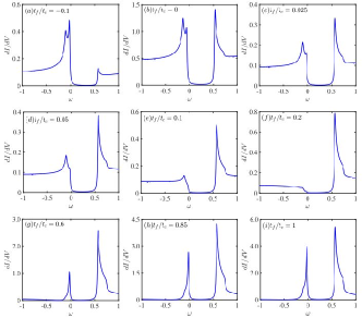
Figure 7: The STM spectra of the KHM versus the ratio of amplitudes $t_{f}/t_{c}$ for NN electron hopping but with NNN hole hopping, where $t=1,t_{1}/t=0.3,n_{c}=0.9,J_{K}=2.5$. The ratio of amplitudes $t_{f}/t_{c}$ influences the line-shape of the $dI/dV$.

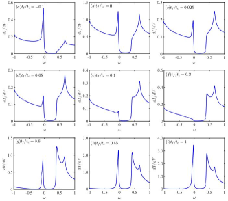
Figure 8: The STM spectra of the KHM versus the ratio of amplitudes $t_{f}/t_{c}$ for NN hole hopping but with NNN electron hopping, where $t=-1,t_{1}/t=0.3,n_{c}=0.9,J_{K}=2.5$. The ratio of amplitudes $t_{f}/t_{c}$ influences the line-shape of the $dI/dV$.

When increasing $t_{f}/t_{c}$, the line-shape changes quickly. Fig. 7 (a) - (c) have three peaks and (h) - (i) have two peaks. There emerges a peak when $\omega>0$, and the peak is increasing versus the $t_{f}/t_{c}$, which is the precursor of the emerging f-electron band.Figgins2010 Fig. 8 (a) - (d) have two peaks and (h) - (i) exist three peaks. Fig. 7 (e) becomes two peaks while Fig. 8 (e) begins to have three peaks. In the subplots (f) of Figs. 7 - 8, the left resonance peak nearly vanishes, which means the suppression of the differential conductance around the Fermi energy.Figgins2010

We also give the STM spectra of the different Kondo coupling $J_{K}$ as shown in Figs. 9 - 10. Compared with Figs. 7 - 8, the line-shape varies versus $t_{f}/t_{c}$. There also exist the suppression of the differential conductance around the Fermi energy as shown in the subplots (e) of Figs. 9 - 10. The subplots (b) of Figs. 7 - 10 are the DOS of the conduction electron.

Among those figures, the gap is increasing versus the Heisenberg coupling $J_{H}$ and the Kondo coupling $J_{K}$. STM line-shape of the differential conductance $dI/dV$ is mainly influenced by the ratio of $t_{f}/t_{c}$, the larger $t_{f}/t_{c}$ induces larger peak. The line-shape of the differential conductance $dI/dV$ emerges much f-electron information versus the ratio of $t_{f}/t_{c}$. We also find that those spectra are qualitatively similar with CeCoIn₅.aynajian2012visualizing These results show that the existence of two resonance peaks structure in differential conductance as Refs. Figgins2010 ; Maltseva2009 , which gives the insight to the heavy-fermion compounds by STM to examine the correlated electrons with high energy and spatial resolutions.Aynajian2012

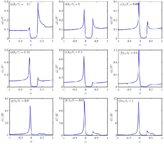
Figure 9: The STM spectra of the KHM versus the ratio of amplitudes $t_{f}/t_{c}$ for NN electron hopping but with NNN hole hopping, where $t=1,t_{1}/t=0.3,n_{c}=0.9,J_{K}=2$. The ratio of amplitudes $t_{f}/t_{c}$ influences the shape-line of the $dI/dV$.

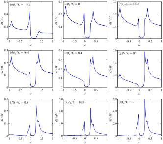
Figure 10: The STM spectra of the KHM model versus the ratio of amplitudes $t_{f}/t_{c}$ for NN hole hopping but with NNN electron hopping, where $t=-1,t_{1}/t=0.3,n_{c}=0.9,J_{K}=2$. The ratio of amplitudes $t_{f}/t_{c}$ influences the shape-line of the $dI/dV$.

V Conclusion and perspective

In summary, we have investigated the KHM on triangular lattice with the fermionic large-N mean-field theory at the case of the NN electron hopping with NNN hole hopping and the case of the NN hole hopping and NNN electron hopping. At the heavy-fermion liquid state, the Heisenberg antiferromagnetic interaction ($J_{H}$) induces twice FS topology change, i.e. the Lifshitz transition, where goes through the continuous transition. In two cases, the conduction electron DOS is changed after Lifshitz transition, the gap is influenced by the Kondo coupling $J_{K}$ and the Heisenberg interaction $J_{H}$. The line-shape of the differential conductance $dI/dV$ shows that the existence of two resonance peaks structure in differential conductance as Refs. Figgins2010 ; Maltseva2009 .The short-range antiferromagnetic correlation coupling $J_{H}$, the ratio of the amplitudes of the f-electron to the amplitude of the the conduction electron $t_{f}/t_{c}$, and the Kondo correlation $J_{K}$ influence the shape-line of the differential conductance $dI/dV$, which gives the insight to detect the heavy-fermion compounds STM spectra for examining the correlated electrons with high energy and spatial resolutions.Aynajian2012

Owing to some triangular heavy-fermion compounds like YbAgGePhysRevB.71.054408 ; PhysRevLett.110.176402 ; PhysRevB.69.014415 ; PhysRevLett.111.116401 and YbAl₃C₃PhysRevB.87.220406 ; PhysRevB.85.144416 have been found, we expect that our results may be confirmed by many FS measurements (Hall coefficient, de Haas-van Alphen measurements, angle-resolved photoemission spectroscopy, quasiparticle interference and STM spectrum experiments) in those compounds.

References

- (1) I. Lifshitz et al., Sov. Phys. JETP 11, 1130 (1960).
- (2) M. R. Norman, J. Lin, and A. J. Millis, Phys. Rev. B 81, 180513 (2010).
- (3) S. Benhabib, A. Sacuto, M. Civelli, I. Paul, M. Cazayous, Y. Gallais, M.-A. M asson, R. D. Zhong, J. Schneeloch, G. D. Gu, D. Colson, and A. Forget, Phys. Rev. Lett. 114, 147001 (2015).
- (4) D. LeBoeuf, N. Doiron-Leyraud, B. Vignolle, M. Sutherland, B. J. Ramshaw, J. Levallois, R. Daou, F. Lalibert , O. Cyr-Choini re, J. Chang, Y. J. Jo, L. Balicas, R. Liang, D. A. Bonn, W. N. Hardy, C. Proust, and L. Taillefer, Phys. Rev. B 83, 054506 (2011).
- (5) S. N. Khan and D. D. Johnson, Phys. Rev. Lett. 112, 156401 (2014).
- (6) H. Hodovanets, Y. Liu, A. Jesche, S. Ran, E. D. Mun, T. A. Lograsso, S. L. Bud ko, and P. C. Canfield, Phys. Rev. B 89, 224517 (2014).
- (7) K. Cho, M. Konczykowski, S. Teknowijoyo, M. A. Tanatar, Y. Liu, T. A. Lograsso, W. E. Straszheim, V. Mishra, S. Maiti, P. J. Hirschfeld, et al., Science advances 2, e1600807 (2016).
- (8) Y. Liu and T. A. Lograsso, Phys. Rev. B 90, 224508 (2014).
- (9) T. Sato, K. Nakayama, Y. Sekiba, P. Richard, Y.-M. Xu, S. Souma, T. Takahashi, G. F. Chen, J. L. Luo, N. L. Wang, and H. Ding, Phys. Rev. Lett. 103, 047002 (2009).
- (10) K. Nakayama, T. Sato, P. Richard, Y.-M. Xu, T. Kawahara, K. Umezawa, T. Qian, M. Neupane, G. F. Chen, H. Ding, and T. Takahashi, Phys. Rev. B 83, 020501 (2011).
- (11) W. Malaeb, T. Shimojima, Y. Ishida, K. Okazaki, Y. Ota, K. Ohgushi, K. Kihou, T. Saito, C. H. Lee, S. Ishida, M. Nakajima, S. Uchida, H. Fukazawa, Y. Kohori, A. Iyo, H. Eisaki, C.-T. Chen, S. Watanabe, H. Ikeda, and S. Shin, Phys. Rev. B 86, 165117 (2012).
- (12) N. Xu, P. Richard, X. Shi, A. van Roekeghem, T. Qian, E. Razzoli, E. Rienks, G.-F. Chen, E. Ieki, K. Nakayama, T. Sato, T. Takahashi, M. Shi, and H. Ding, Phys. Rev. B 88, 220508 (2013).
- (13) C. Liu, T. Kondo, R. M. Fernandes, A. D. Palczewski, E. D. Mun, N. Ni, A. N. Thaler, A. Bostwick, E. Rotenberg, J. Schmalian, et al., Nature Physics 6, 419 (2010).
- (14) G. Volovik, Low Temperature Physics 43, 47 (2017).
- (15) I. V. Iorsh, K. Dini, O. V. Kibis, and I. A. Shelykh, Phys. Rev. B 96, 155432 (2017).
- (16) R. Daou, C. Bergemann, and S. R. Julian, Phys. Rev. Lett. 96, 026401 (2006).
- (17) N. Harrison, S. E. Sebastian, C. H. Mielke, A. Paris, M. J. Gordon, C. A. Swenson, D. G. Rickel, M. D. Pacheco, P. F. Ruminer, J. B. Schillig, J. R. Sims, A. H. Lacerda, M.-T. Suzuki, H. Harima, and T. Ebihara, Phys. Rev. Lett. 99, 056401 (2007).
- (18) K. M. Purcell, D. Graf, M. Kano, J. Bourg, E. C. Palm, T. Murphy, R. McDonald, C. H. Mielke, M. M. Altarawneh, C. Petrovic, R. Hu, T. Ebihara, J. Cooley, P. Schlottmann, and S. W. Tozer, Phys. Rev. B 79, 214428 (2009).
- (19) P. Schlottmann, Phys. Rev. B 83, 115133 (2011).
- (20) H. Pfau, R. Daou, S. Lausberg, H. R. Naren, M. Brando, S. Friedemann, S. Wirth, T. Westerkamp, U. Stockert, P. Gegenwart, C. Krellner, C. Geibel, G. Zwicknagl, and F. Steglich, Phys. Rev. Lett. 110, 256403 (2013).
- (21) D. Aoki, G. Seyfarth, A. Pourret, A. Gourgout, A. Mc-Collam, J. A. N. Bruin, Y. Krupko, and I. Sheikin, Phys. Rev. Lett. 116, 037202 (2016).
- (22) S. Paschen, T. L hmann, S. Wirth, P. Gegenwart, O. Trovarelli, C. Geibel, F. Steglich, P. Coleman, and Q. Si, Nature 432, 881 (2004).
- (23) G.-M. Zhang, Y.-H. Su, and L. Yu, Phys. Rev. B 83, 033102 (2011).
- (24) Y. Zhong, L. Zhang, H.-T. Lu, and H.-G. Luo, The European Physical Journal B 88, 238 (2015).
- (25) Y. Liu, G.-M. Zhang, and Y. Lu, Chin. Phys. Lett. 31, 087102 (2014).
- (26) M. Bercx and F. F. Assaad, Phys. Rev. B 86, 075108 (2012).
- (27) S. Nandy, N. Mohanta, S. Acharya, and A. Taraphder, Phys. Rev. B 94, 155103 (2016).
- (28) S. Burdin and C. Lacroix, Phys. Rev. Lett. 110, 226403 (2013).
- (29) F. Grandi, A. Amaricci, M. Capone, and M. Fabrizio, Phys. Rev. B 98, 045105 (2018).
- (30) S. K. Sinha, G. H. Lander, S. M. Shapiro, and O. Vogt, Phys. Rev. Lett. 45, 1028 (1980).
- (31) A. Zieba, M. Slota, and M. Kucharczyk, Phys. Rev. B 61, 3435 (2000).
- (32) L. Isaev and I. Vekhter, Phys. Rev. Lett. 110, 026403 (2013).
- (33) S. Hoshino and Y. Kuramoto, Phys. Rev. Lett. 111, 026401 (2013).
- (34) M. Z. Asadzadeh, F. Becca, and M. Fabrizio, Phys. Rev. B 87, 205144 (2013).
- (35) A. Hackl and M. Vojta, Phys. Rev. B 77, 134439 (2008).
- (36) A. Hackl and M. Vojta, Phys. Rev. Lett. 106, 137002 (2011).
- (37) S. L. Bud ko, E. Morosan, and P. C. Canfield, Phys. Rev. B 71, 054408 (2005).
- (38) J. K. Dong, Y. Tokiwa, S. L. Bud ko, P. C. Canfield, and P. Gegenwart, Phys. Rev. Lett. 110, 176402 (2013).
- (39) S. L. Bud ko, E. Morosan, and P. C. Canfield, Phys. Rev. B 69, 014415 (2004).
- (40) Y. Tokiwa, M. Garst, P. Gegenwart, S. L. Bud ko, and P. C. Canfield, Phys. Rev. Lett. 111, 116401 (2013).
- (41) D. D. Khalyavin, D. T. Adroja, P. Manuel, A. Daoud-Aladine, M. Kosaka, K. Kondo, K. A. McEwen, J. H. Pixley, and Q. Si, Phys. Rev. B 87, 220406 (2013).
- (42) K. Hara, S. Matsuda, E. Matsuoka, K. Tanigaki, A. Ochiai, S. Nakamura, T. Nojima, and K. Katoh, Phys. Rev. B 85, 144416 (2012).
- (43) P. Aynajian, E. H. da Silva Neto, A. Gyenis, R. E. Baumbach, J. Thompson, Z. Fisk, E. D. Bauer, and A. Yazdani, Nature 486, 201 (2012).
- (44) P. Coleman and N. Andrei, Journal of Physics: Condensed Matter 1, 4057 (1989).
- (45) J. Arispe, B. Coqblin, and C. Lacroix, Physica B: Condensed Matter 206, 255 (1995).
- (46) J. Iglesias, C. Lacroix, J. Arispe, and B. Coqblin, Physica B: Condensed Matter 223, 160 (1996).
- (47) C. Lacroix, J. Iglesias, J. Arispe, and B. Coqblin, Physica B: Condensed Matter 230, 503 (1997).
- (48) N. Read and D. M. Newns, Journal of Physics C: Solid State Physics 16, 3273 (1983).
- (49) Y. Liu, H. Li, G.-M. Zhang, and L. Yu, Phys. Rev. B 86, 024526 (2012).
- (50) J. Figgins and D. K. Morr, Phys. Rev. Lett. 104, 187202 (2010).
- (51) A. Damascelli, Z. Hussain, and Z.-X. Shen, Rev. Mod. Phys. 75, 473 (2003).
- (52) O. Fischer, M. Kugler, I. Maggio-Aprile, C. Berthod, and C. Renner, Rev. Mod. Phys. 79, 353 (2007).
- (53) S. Kirchner, S. Paschen, Q. Chen, S. Wirth, D. Feng, J. D. Thompson, and Q. Si, arXiv:1810.13293 (2018).
- (54) J. Tersoff and D. R. Hamann, Phys. Rev. B 31, 805 (1985).
- (55) K. Kummer, S. Patil, A. Chikina, M. Guttler, M. Hoppner, A. Generalov, S. Danzenbacher, S. Seiro, A. Hannaske, C. Krellner, Y. Kucherenko, M. Shi, M. Radovic, E. Rienks, G. Zwicknagl, K. Matho, J. W. Allen, C. Laubschat, C. Geibel, and D. V. Vyalikh, Phys. Rev. X 5, 011028 (2015).
- (56) S. Paschen, T. Luhmann, S. Wirth, P. Gegenwart, O. Trovarelli, C. Geibel, F. Steglich, P. Coleman, and Q. Si, Nature 432, 881 (2004).
- (57) M. Allan, F. Massee, D. Morr, J. Van Dyke, A. Rost, A. Mackenzie, C. Petrovic, and J. Davis, Nature physics 9, 468 (2013).
- (58) B. B. Zhou, S. Misra, E. H. da Silva Neto, P. Aynajian, R. E. Baumbach, J. Thompson, E. D. Bauer, and A. Yazdani, Nature physics 9, 474 (2013).
- (59) J. D. Thompson and Z. Fisk, Journal of the Physical Society of Japan 81, 011002 (2012).
- (60) M. Maltseva, M. Dzero, and P. Coleman, Phys. Rev. Lett. 103, 206402 (2009).
- (61) Pegor Aynajian, Eduardo H da Silva Neto, Andr s Gyenis et al., Nature 486, 201 (2012).