KMT-2019-BLG-1339L: an M Dwarf with a Giant Planet or a Companion Near the Planet/Brown Dwarf Boundary

Abstract

We analyze KMT-2019-BLG-1339, a microlensing event with an obvious but incompletely resolved brief anomaly feature around the peak of the light curve. Although the origin of the anomaly is identified to be a companion to the lens with a low mass ratio $q$, the interpretation is subject to two different degeneracy types. The first type is the ambiguity in $\rho$, representing the angular source radius scaled to the angular radius of the Einstein ring, $\theta_{\rm E}$, and the other is the $s\leftrightarrow s^{-1}$ degeneracy. The former type, ‘finite-source degeneracy’, causes ambiguities in both $s$ and $q$, while the latter induces an ambiguity only in $s$. Here $s$ denotes the separation (in units of $\theta_{\rm E}$) in projection between the lens components. We estimate that the lens components have masses $(M_{1},M_{2})\sim(0.27^{+0.36}_{-0.15}~{}M_{\odot},11^{+16}_{-7}~{}M_{\rm J})$ and $\sim(0.48^{+0.40}_{-0.28}~{}M_{\odot},1.3^{+1.1}_{-0.7}~{}M_{\rm J})$ according to the two solutions subject to the finite-source degeneracy, indicating that the lens comprises an M dwarf and a companion with a mass around the planet/brown dwarf boundary or a Jovian-mass planet. It is possible to lift the finite-source degeneracy by conducting future observations utilizing a high resolution instrument because the relative lens-source proper motion predicted by the solutions are widely different.

1. Introduction

A microlensing planet is, in general, detected through a short-lasting anomaly appearing in the lensing light curve of the host (Mao & Paczyński, 1991). Due to the brief nature of a planetary signal, one is often confronted with cases in which the coverage of the signal is incomplete due to various causes such as insufficient cadence of observations, bad weather, time gap between observatories, etc.

Interpreting short-term microlensing signals with incomplete coverage can result in a degeneracy problem, in which multiple solutions with different combinations of lensing parameters can describe an observed anomaly, leading to multiple interpretations of the signal. There have been reports of such cases caused by various types of degeneracy. The first case was reported by Skowron et al. (2018) for OGLE-2017-BLG-0373 with a partially covered planetary signal. From the analysis of the light curve, they found a pair of degenerate solutions, in which the folds of the planetary caustic located on the opposite sides with respect to the caustic center were swept by the source with nearly equal offsets from the caustic center. The two solutions resulting from this “caustic-chiral degeneracy” have substantially different values of the planet/host mass ratio $q$, although they have similar planet-host separations (in projection) $s$ (scaled to the angular Einstein radius $\theta_{\rm E}$). This mode of degeneracy was also identified by Hwang et al. (2018a), when they analyzed KMT-2016-BLG-0212 with a partially covered planetary signal. The second case of a discrete degeneracy was identified from the analysis of OGLE-2017-BLG-0173 (Hwang et al., 2018b), for which the anomaly was insufficiently covered with a gap in the data. This “Hollywood degeneracy” yielded two solutions, in which the source fully encompassed the planetary caustic according to one solution, and the source surrounded only one caustic side according to the other solution. This degeneracy causes an ambiguity in determining $q$. The third case, found from OGLE-2018-BLG-0740 with a partially covered planetary signal, was reported by Han et al. (2019). For this event, the degenerate solutions yielded different values of $\rho$, representing the angular radius of the source $\theta_{*}$ normalized to $\theta_{\rm E}$ (normalized source radius), and this caused ambiguities in both $s$ and $q$. Considering that planetary signals for an important fraction of microlensing events would be detected with incomplete coverage, it is important to identify various types of degeneracies and investigate their origins to correctly interpret planetary signals in future analyses.

Here we analyze the partially covered short-term anomaly feature that appears in the lensing light curve of KMT-2019-BLG-1339. We find that interpreting the anomaly is subject to two different types of degeneracy, and we investigate the origins of the degeneracies.

The organization of the paper is as follows. The data acquired from observing the lensing event are addressed in Section 2. In Section 3, we mention the procedure of modeling conducted to interpret the observed anomaly. We also mention the types of degeneracy identified from modeling. We estimate the $\theta_{\rm E}$ values corresponding to the degenerate solutions in Section 4. Estimation of the lens masses and distances for the degenerate solutions is provided in Section 5. In Section 6, we suggest a method to lift the identified degeneracy. Summary of the findings and conclusion are given in Section 7.

2. Observations

The source star of the lensing event KMT-2019-BLG-1339/OGLE-2019-BLG-1019 lies in the Galactic bulge field. The coordinates of the source are $({\rm R.A.},{\rm decl.})_{\rm J2000}\equiv(17:42:58.42,-25:34:26.1)$, corresponding to $(l,b)=(2^{\circ}\hskip-2.0pt.559,2^{\circ}\hskip-2.0pt.260)$. The apparent brightness of the source remained constant before lensing with an $I$-band baseline magnitude of $I\sim 20.4$.

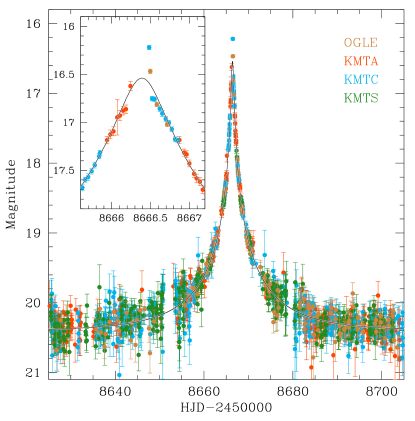
Figure 1.— Photometric data around KMT-2019-BLG-1339. The curve plotted over the data points is the 1L1S model. The zoom of the peak region is shown in the inset.

The Korea Microlensing Telescope Network (KMTNet: Kim et al., 2016) experiment first detected the event on 2019-06-26, which corresponds to ${\rm HJD}^{\prime}\equiv{\rm HJD}-2450000=8660$, using the alert-finder system (Kim et al., 2018). At the time of finding, the source was brighter than the baseline magnitude by $\Delta I\sim 0.86$ magnitude. Five days later, the event was independently found by another lensing survey of the Optical Gravitational Lensing Experiment (OGLE: Udalski et al., 2015). The event was designated as KMT-2019-BLG-1339 and OGLE-2019-BLG-1019 by the individual surveys. Hereafter, we use KMT-2019-BLG-1339 as a representative name of the event. The KMTNet survey utilizes three identical telescopes, each with a 1.6 m aperture and mounted with a camera having a $4~{}{\rm deg}^{2}$ field of view. The telescopes are located in three different continents: the South African Astronomical Observatory in South Africa (KMTS), the Cerro Tololo Inter-American Observatory in Chile (KMTC), and the Siding Spring Observatory in Australia (KMTA). The OGLE survey utilized the Warsaw telescope, with a 1.3 m aperture, at the Las Campanas Observatory in Chile, and the camera mounted on the telescope has a $1.4~{}{\rm deg}^{2}$ field of view. The source was located in the KMTNet BLG19 and OGLE BLG652.26 fields, toward which observations by the individual surveys were conducted with $\sim 1~{}{\rm hr}$ and $\sim 2~{}{\rm hr}$ cadences, respectively. For both surveys, observations were conducted primarily in the $I$ band, and observations in the $V$ band were done to obtain a subset of data to measure the source color. The data used in the analysis lie in the time range of $8620\lesssim{\rm HJD}^{\prime}\lesssim 8720$.

Reduction of data is done with the photometry pipelines of the KMTNet (Albrow et al., 2009) and OGLE (Woźniak, 2000) surveys. These pipelines commonly employ the difference image analysis (DIA) algorithm (Alard & Lupton, 1998; Tomaney & Crotts, 1996), that is developed for optimal crowded field photometry. For a subset of KMTC $I$- and $V$-band images taken around the lensing magnifications, we carry out extra photometry with the use of the pyDIA software (Albrow, 2017) to measure the source color. The ranges of the pyDIA data sets are $8566.9\leq{\rm HJD}^{\prime}\leq 8728.5$ and $8642.7\leq{\rm HJD}^{\prime}\leq 8713.5$ for the $I$ and $V$-band data sets, respectively. We note that the pyDIA photometry measures the flux itself, while the DIA photometry measures the difference in flux from the baseline. Because the pyDIA photometry is affected by blended light, the photometry quality is poorer than that of the DIA photometry. Nevertheless, data sets processed by the pyDIA photometry are needed to estimate the apparent magnitudes of the lensing event and the color of the source star. Detailed process of the source color estimation is discussed in Section 4.

We reevaluate the errors bars of data from the photometry pipelines. Following the recipe addressed in Yee et al. (2012), this process is done by

$$\sigma=k(\sigma_{0}^{2}+\sigma_{\rm min}^{2})^{1/2}.$$ (1)

Here $\sigma_{0}$ denotes the error bar estimated from the pipeline, $\sigma_{\rm min}$ is the scatter of data, and $k$ is a factor used to make $\chi^{2}$ per degree of freedom become unity. Table 1 shows the values of $k$ and $\sigma_{\rm min}$ together with the numbers of data points, $N_{\rm data}$, in the individual data sets.

Figure 1 shows the photometry data around the time of the lensing event. Different colors are used to designate the telescopes used for the data acquisition. The solid curve plotted over the data points is the model found under a standard single-lens single-source (1L1S) interpretation. According to the 1L1S model, the event is magnified with a moderately high magnification of $A_{\rm peak}\sim 62$ at the peak, and the event timescale is $t_{\rm E}\sim 17.6$ days. We check the feasibility of measuring the annual microlens parallax $\pi_{\rm E}$ (Gould, 1992), but $\pi_{\rm E}$ cannot be securely estimated mostly because of the short event timescale relative to the orbital period of the Earth.

Table 1Numbers of data points

Data set	$k$	$\sigma_{\rm min}$	$N_{\rm data}$
KMTA	1.068	0.030	355
KMTC	1.054	0.020	569
KMTS	1.034	0.040	426
OGLE	1.082	0.020	125

3. Light Curve Analysis

Although the light curve of the event seemingly looks like that of a 1L1S event, a close inspection reveals that the peak part of the light curve exhibits small but noticeable deviations from the model. See the inset of Figure 1 showing the zoom of the peak region.

Figure 2 shows the residuals from the 1L1S model around the peak. The residuals exhibit the following characteristics. First, the three data points at ${\rm HJD}^{\prime}=8666.242$ (KMTA), 8666.483 (KMTC), and 8666.497 (OGLE) exhibit discontinuous deviations from the 1L1S model. Second, the KMTA data points just before the peak (in the region $8666.0\lesssim{\rm HJD}^{\prime}\lesssim 8666.2$) and the OGLE and KMTC data points just after the peak (in the region $8666.5\lesssim{\rm HJD}^{\prime}\lesssim 8666.7$) exhibit continuous negative deviations from the 1L1S model. We note that the coverage of the major part of the anomaly is incomplete due to the $\sim 5.8$ hr time gap between the last point of the KMTA data and the first point of the KMTC data taken on 2019-07-01. The gap corresponded to a night time in Africa, but observations by KMTS could not be conducted due to the bad weather.

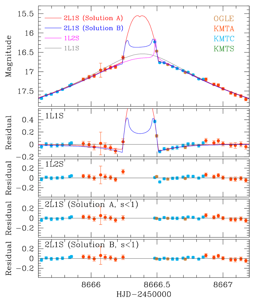
Figure 2.— Model curves under various interpretations of the lens system, including 1L1S , 1L2S, and 2L1S models. For the 2L1S interpretation, we present two models, solution “A” (with $s<1.0$) and “B” ($s<1.0$), resulting from the discrete degeneracy. The residuals from the tested models are shown in the lower panels. The two curves drawn on the 1L1S residuals (second panel) are the differences between the 2L1S (red for solution A and blue for solution B) and 1L1S models.

The characteristics of the deviations from the 1L1S model suggest that there may exist a caustic in the central magnification zone induced by a companion to the lens. With such a caustic, the three data points exhibiting discontinuous deviations would be explained by the caustic crossings of the source, and the data points with smooth negative deviations before and after the peak would be explained by the negative excess magnification in the regions immediately outside the fold of the caustic. If this interpretation is correct, the caustic should be very small because the time gap between the two successive caustic crossings is very short.

We check the presence of a central caustic by modeling the light curve under the binary lens interpretation (2L1S model). A 1L1S light curve is defined by three parameters, which are the time of the lens-source minimum separation, $t_{0}$, the impact parameter, $u_{0}$, and the event timescale, $t_{\rm E}$. A 2L1S modeling demands extra parameters of $(s,q,\alpha)$. Here $\alpha$ denotes the source trajectory angle, which is defined as the angle between the source trajectory and the line connecting the binary lens components. Because the three discontinuous points are believed to lie on the caustic-crossing parts, during which lensing magnifications experience finite-source effects. To account for these effects, we conduct modeling with the inclusion of an extra parameter $\rho\equiv\theta_{*}/\theta_{\rm E}$ (normalized source radius). Here $\theta_{*}$ represents the angular size of the source radius. We compute finite-source magnifications using the method of Dong et al. (2006), which utilizes the ray-shooting algorithm. We take the limb-darkening effect into consideration in computing finite magnifications. We choose the limb-darkening coefficients considering the source type, which is a late F-type main-sequence star. Details of the source type determination are mentioned in Section 4. We assume that the surface brightness varies as $S\propto 1-\Gamma_{\lambda}(1-3\cos\psi/2)$, in which $\Gamma$ denotes the limb-darkening coefficient and $\psi$ is the angle between the radial direction from the source center and the line of sight toward the source center. We adopt $\Gamma_{I}=0.37$ and $\Gamma_{V}=0.52$ from the Claret (2000) catalog.

Implementing light curve modeling is done in two rounds. In the first-round modeling, we find the parameters $s$ and $q$ using a grid-search approach, while we look for the other parameters utilizing a downhill simplex method based on the Markov Chain Monte Carlo (MCMC) algorithm. In the second-round modeling, we find local minima by inspecting $\Delta\chi^{2}$ map on the grid parameter, $s$ and $q$, space. Each local minima is then further refined from an additional modeling, in this time, by letting all parameters vary. This two-step procedure is useful in identifying degenerate solutions, if they exist.

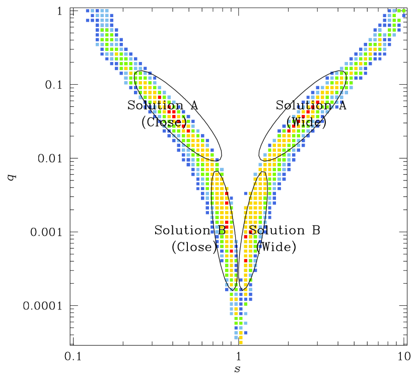
Figure 3.— Four local minima in the $\Delta\chi^{2}$ map on the parameter plane of the binary separation $s$ and mass ratio $q$. The colors of points designate regions with $<1n\sigma$ (red), $<2n\sigma$ (yellow), $<3n\sigma$ (green), and $<4n\sigma$ (blue), where $n=3$.

The 2L1S modeling yields four degenerate local solutions. For visual presentation of the local solutions, we mark the individual degenerate solutions in the $s$–$q$ plane in Figure 3. From the inspection of the map, it is found that the mass ratios of one pair of the solutions are $q\sim 4\times 10^{-2}$ and those of the other pair are $q\sim 2.5\times 10^{-3}$. Hereafter, we refer to the solutions with $q\sim 4\times 10^{-2}$ and $q\sim 2.5\times 10^{-3}$ as solutions “A” and “B”, respectively. For each pair, we identify another pair of solutions: one with $s<1$ (close solution) and the other with $s>1$ (wide solution). The latter degeneracy is caused by the close/wide degeneracy (Griest & Safizadeh, 1998; Dominik, 1999; An, 2005). With $\chi^{2}$ differences among the solutions being merely $\Delta\chi^{2}\sim 1.2$, we find that resolving the degeneracies is difficult based on the photometric data alone.

It is found that the 2L1S solutions well describe the observed light curve including the peak part exhibiting deviations from the 1L1S model. The 2L1S models provides a better fit than the 1L1S model by $\Delta\chi^{2}\sim 290$. The model curves of the solutions A (with $s<1$) and B ($s<1$) are shown in the top panel of Figure 2, and the residuals from the individual models are presented in the bottom two panels. In the second panel, we present the difference between the 2L1S and 1L1S models: red curve for the solution A (with $s<1$) and blue curve for the solution B ($s<1$). For both solutions A and B, the deviations from the 1L1S solution are explained by the caustic crossings, as expected. However, it is found that the model curves of the two degenerate solutions are substantially different in the region between the times of the caustic crossings. The degeneracy could have been resolved if there existed a few data points between the times of the caustic crossings, implying that the degeneracy is accidentally caused by the gap in the data.

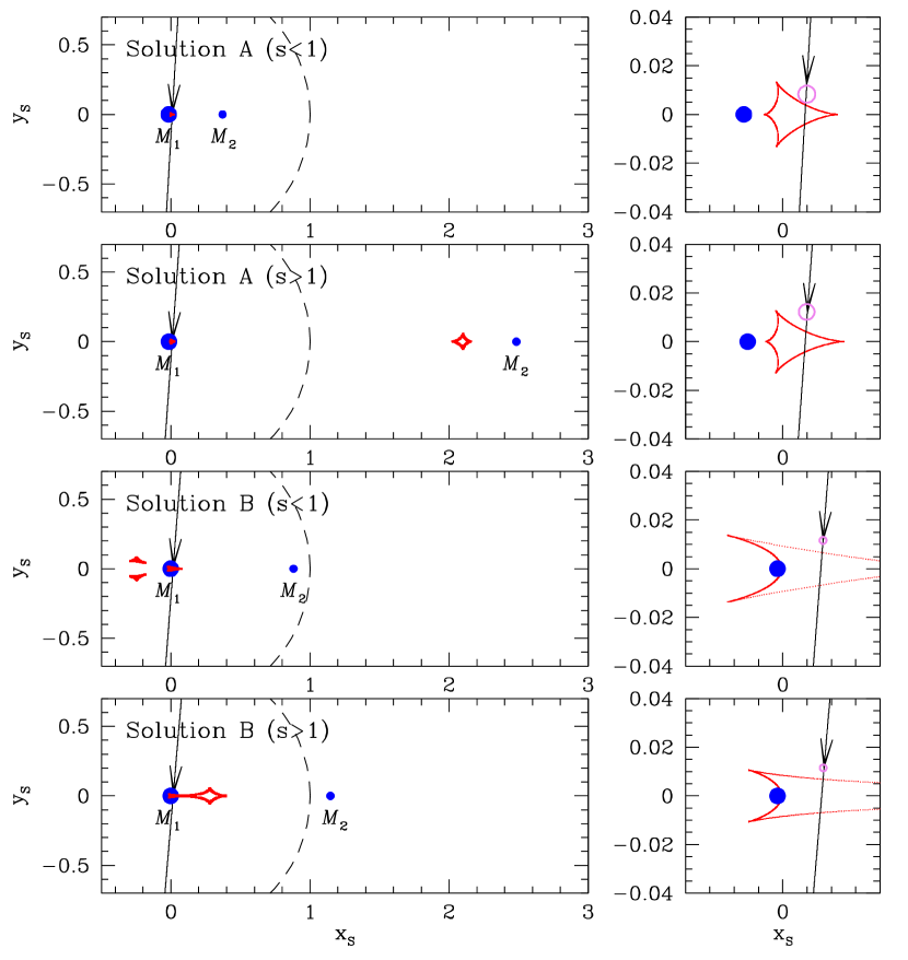
Figure 4.— Configurations of the lens and source for the four local solutions from the 2L1S modeling. In each panel, the two blue dots, labeled by $M_{1}$ and $M_{2}$, denote the lens positions and the cuspy closed figures are the caustics. The solid line and the arrow on the line indicate the trajectory and the direction of the source motion, respectively. The small pink circle on the source trajectory is drawn to compare the source size with the caustic size. The dashed circle is the Einstein ring.

Table 2Lensing parameters of various models

Parameter	1L2S	2L1S (Solution A)		2L1S (Solution B)
		Close	Wide	Close	Wide
$\chi^{2}$	1499.5	1474.5	1474.3	1473.3	1473.8
$t_{0}$ (${\rm HJD}^{\prime}$)	$8666.395\pm 0.004$	$8666.378\pm 0.004$	$8666.379\pm 0.004$	$8666.391\pm 0.003$	$8666.393\pm 0.003$
$u_{0}$ ($10^{-2}$)	$2.002\pm 0.129$	$0.913\pm 0.081$	$0.922\pm 0.083$	$1.560\pm 0.089$	$1.593\pm 0.096$
$t_{\rm E}$ (days)	$16.43\pm 0.67$	$17.23\pm 0.84$	$17.66\pm 0.90$	$16.70\pm 0.68$	$16.45\pm 0.70$
$s$	–	$0.39\pm 0.05$	$2.50\pm 0.41$	$0.88\pm 0.03$	$1.15\pm 0.04$
$q$ ($10^{-3}$)	–	$43.03\pm 13.94$	$37.48\pm 15.22$	$2.47\pm 0.66$	$2.50\pm 0.77$
$\alpha$ (rad)	–	$4.771\pm 0.019$	$4.784\pm 0.016$	$4.790\pm 0.014$	$4.797\pm 0.015$
$\rho$ ($10^{-3}$)	–	$3.49\pm 0.61$	$3.20\pm 0.54$	$1.42\pm 0.32$	$1.38\pm 0.30$
$t_{0,2}$	$8666.487\pm 0.003$	–	–	–	–
$u_{0,2}$ ($10^{-2}$)	$0.000\pm 0.022$	–	–	–	–
$\rho_{2}$ ($10^{-3}$)	$0.39\pm 0.21$	–	–	–	–
$q_{F}$	$0.006\pm 0.002$	–	–	–	–
$f_{\rm s,OGLE}$	$0.068\pm 0.003$	$0.063\pm 0.003$	$0.063\pm 0.004$	$0.066\pm 0.003$	$0.067\pm 0.003$
$f_{\rm b,OGLE}$	$0.042\pm 0.003$	$0.047\pm 0.003$	$0.046\pm 0.003$	$0.044\pm 0.003$	$0.043\pm 0.003$

Note. — ${\rm HJD}^{\prime}\equiv{\rm HJD}-2450000$.

The lensing parameters and the $\chi^{2}$ values of the fits for the individual 2L1S solutions are listed in Table 2. The mass ratios of the B solutions, $q\sim 2.5\times 10^{-3}$, indicate that the companion to the lens has a planetary mass. For the A solutions with $q\sim 4\times 10^{-2}$, on the other hand, the nature of the lens companion is uncertain just based the mass ratio because the mass could be below or above the lower mass limit of brown dwarfs (BDs), $\sim 13~{}M_{\rm J}$ (Boss et al., 2007), depending on the mass of the primary. The $f_{s,I}$ and $f_{b,I}$ listed in the table denote the values of the $I$-band flux for the source and blend, respectively. Following the OGLE photometry system, the flux is set to be unity for a star with $I=18$. Besides the mass ratios, we point out that the normalized source radii estimated from the solutions A and B are substantially different: $\rho\sim 3.3\times 10^{-3}$ (solutions A) and $\rho\sim 1.4\times 10^{-3}$ (solutions B). As a result, the model curve of the solution B exhibits a well-defined “U”-shape trough feature between the caustic crossings, while the feature in the model curve of the solution A is smeared out by severe finite-source effects.

The configurations of the source and lens for the individual 2L1S solutions are shown in Figure 4. For each solution, the left panel is presented to show the locations of both lens components (blue dots tagged by $M_{1}$ and $M_{2}$), and the right panel is given to show the central magnification region. For solutions B, the lower-mass lens component lies near the Einstein ring (dashed circle centered at the origin). For solutions A, on the other hand, the separation of the lens companion from the Einstein ring is relatively big. It is found that the central caustics for each close-wide pair of the solutions appear to be similar to each other, and this results in the close/wide degeneracy. In contrast, the caustics between the solutions A and B appear to be substantially different. The solid line and the arrow on the line indicate the trajectory and the direction of the source motion, respectively. It shows that the anomaly arises by the source passage through the central caustic almost at a right angle.

The mode of the degeneracy between the solutions A and B is similar to the degeneracy mode identified for OGLE-2018-BLG-0740 (Han et al., 2019). The similarity between the two events is that the coverage of the anomaly is incomplete, and this causes the ambiguity in $\rho$. For OGLE-2018-BLG-0740, the “U”-shape trough feature is covered, but the caustic-crossing parts are poorly covered. For KMT-2019-BLG-1339, on the other hand, there are three data points, one in rising and two in falling parts, in the caustic-crossing parts, but the “U”-shape trough feature is not covered. This suggests that the finite-source degeneracy can arise when the coverage of an anomaly is incomplete.

A short-duration anomaly can also be produced by a subset of binary-source (1L2S) events (Gaudi, 1998; Gaudi & Han, 2004; Shin et al., 2019), and thus we conduct an additional modeling with the 1L2S interpretation. Similar to the 2L1S case, a 1L2S modeling requires to include extra parameters in addition to those of the 1L1S modeling. According to the parameterization of Hwang et al. (2013), these extra parameters are $t_{0,2}$, $u_{0,2}$, $\rho_{2}$, and $q_{F}$, which represent the time of the closest lens approach to the source companion, the impact parameter of the source companion motion, the normalized radius of the source companion, and the flux ratio between the binary source stars, respectively.

The best-fit 1L2S model and its residuals are shown in Figure 2. The lensing parameters of the model are listed in Table 2. We note that the lens passes over the surface of the source companion according to the model, but the lens does not transverse the primary source. As a result, the value of $\rho_{2}$ is presented, while the value of $\rho$ is not given. From the comparison of the fits, it is found that the 1L2S gives a better fit than the 1L1S model by $\Delta\chi^{2}\sim 264$, but the fit is worse than the 2L1S model by $\Delta\chi^{2}\sim 26$. Therefore, we conclude that the central perturbation is caused not by a source companion but by a lens companion.

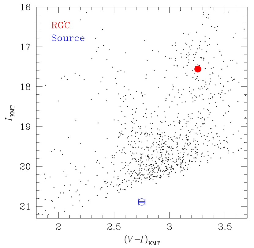
Figure 5.— Color-magnitude diagram of stars around the source of KMT-2019-BLG-1339. The blue empty dot indicates the source position and the red filled dot denotes the centroid of red giant clump (RGC).

4. Angular Einstein Radius

The solutions A and B result in significantly different values of the Einstein radius. This is because these solutions yield substantially different values of $\rho$, from which the value of $\theta_{\rm E}$ is determined, i.e., $\theta_{\rm E}=\theta_{*}/\rho$.

For the $\theta_{\rm E}$ determination, we first estimate $\theta_{*}$. We estimate $\theta_{*}$ using the dereddened color and brightness, $(V-I,I)_{0}$, of the source. Following the recipe of Yoo et al. (2004), we determine the positions of the source and the centroid of red giant clump (RGC) in the color-magnitude diagram (CMD), measure the offset between the source and RGC centroid, and then estimate $(V-I,I)_{0}$ of the source based on the known values of the dereddened color and magnitude of the RGC centroid, $(V-I,I)_{\rm RGC,0}$.

Figure 5 shows the instrumental CMD of stars in the vicinity of the source, and the locations of the source, at $(V-I,I)$, and the RGC centroid, at $(V-I,I)_{\rm RGC}$. The CMD construction and $(V-I,I)$ estimation are based on the KMTC data set reduced using the same pyDIA photometry. We note that the location of the blend is not marked because the color cannot be determined due to the poor $V$-band photometry. The measured values of the color and magnitude are $(V-I,I)=(2.75\pm 0.04,20.89\pm 0.01)$ and $(V-I,I)_{\rm RGC}=(3.26,17.56)$ for the source and RGC centroid, respectively. We calibrate the color and magnitude of the source star using its offsets from the RGC centroid, $\Delta(V-I,I)$, by using the relation

$$(V-I,I)_{0}=(V-I,I)_{\rm RGC,0}+\Delta(V-I,I),$$ (2)

We adopt $(V-I,I)_{\rm RGC,0}=(1.06,14.32)$ from Bensby et al. (2013) and Nataf et al. (2013). From the process, we find $(V-I,I)_{0}=(0.55\pm 0.04,17.65\pm 0.01)$. These values point out that the lensing event occurred on a bulge main sequence with a late F spectral type. After this calibration process, we apply the color-color relation of Bessell & Brett (1988) to derive $V-K$ color, and then use the the Kervella et al. (2004) relation between color and surface-brightness to derive $\theta_{*}$. From this process, the angular radius of the source is estimated as

$$\theta_{*}=0.78\pm 0.06~{}\mu{\rm as}.$$ (3)

Table 3Angular Einstein radius and relative proper motion

Quantity	Solution A	Solution B
$\theta_{\rm E}$ (mas)	$0.22\pm 0.04$	$0.55\pm 0.13$
$\mu$ (mas yr-1)	$4.76\pm 0.92$	$12.08\pm 2.89$

Table 4Physical lens parameters

Parameter	Solution A		Solution B
	Close	Wide	Close	Wide
$M_{1}$ $(M_{\odot})$	$0.27^{+0.36}_{-0.15}$	$0.26^{+0.35}_{-0.14}$	$0.48^{+0.40}_{-0.28}$	$0.49^{+0.40}_{-0.28}$
$M_{2}$ $(M_{\rm J})$	$12.2^{+16.1}_{-6.7}$	$10.7^{+14.0}_{-5.8}$	$1.25^{+1.04}_{-0.73}$	$1.27^{+1.05}_{-0.74}$
$D_{\rm L}$ (kpc)	$7.15^{+1.06}_{-1.25}$	$7.21^{+1.04}_{-1.22}$	$6.12^{+1.26}_{-1.60}$	$6.00^{+1.26}_{-1.64}$
$d_{\perp}$ (au)	$0.67^{+0.77}_{-0.55}$	$4.30^{+4.94}_{-3.55}$	$2.15^{+2.59}_{-1.58}$	$2.80^{+3.38}_{-2.07}$

With the measured $\theta_{*}$, we estimate the values of $\theta_{\rm E}$ and $\mu$ by

$$\theta_{\rm E}={\theta_{*}\over\rho};\qquad\mu={\theta_{\rm E}\over t_{\rm E}}$$ (4)

respectively. The values of $\theta_{\rm E}$ and $\mu$ for the solutions A and B are listed in Table 3. To be noted is that the Einstein radius for the solution B, $\sim 0.55$ mas, is bigger than the value estimated from the solution A, $\sim 0.22$ mas, by a factor $\sim 2.5$. The difference in $\theta_{\rm E}$ originates from the difference in the values of $\rho$ estimated from the individual solutions. For the same reason, the $\mu$ value of the solution A, $\sim 4.8~{}{\rm mas}~{}{\rm yr}^{-1}$, is smaller than the value estimated from the solution B, $\sim 12.1~{}{\rm mas}~{}{\rm yr}^{-1}$, by a similar factor.

5. Physical Lens Parameters

The lens mass $M$ and distance $D_{\rm L}$ are uniquely determined by measuring both $\theta_{\rm E}$ and $\pi_{\rm E}$, i.e.,

$$M={\theta_{\rm E}\over\kappa\pi_{\rm E}};\qquad D_{\rm L}={{\rm au}\over\pi_{\rm E}\theta_{\rm E}+\pi_{\rm S}}.$$ (5)

Here $\kappa=4G/(c^{2}{\rm au})$ and $\pi_{\rm S}$ represents the parallax to the source, i.e., $\pi_{\rm S}={\rm au}/D_{\rm S}$. For KMT-2019-BLG-1339, $\theta_{\rm E}$ is measured with a two-fold degeneracy, but $\pi_{\rm E}$ cannot be measured. For the estimations $M$ and $D_{\rm L}$, we, therefore, conduct a Bayesian analysis based on the measured values of $t_{\rm E}$ and $\theta_{\rm E}$.

In the Bayesian analysis, we conduct a Monte Carlo simulation to produce numerous ($2\times 10^{7}$) artificial lensing events. For the individual events, we derive the physical parameters of lenses (including the lens mass $M$, distance $D_{\rm L}$, and transverse lens-source speed $v$) from priors. Lens masses are derived from the mass function of Chabrier (2003) for stellar lenses and from the mass function of Gould (2000) for remnant objects. Locations and motion of the lens and source are derived from the Han & Gould (2003) and Han & Gould (1995) models, respectively. For the individual events produced by the simulation, we compute the timescales, $t_{{\rm E},i}=D_{\rm L}\theta_{\rm E}/v$, and Einstein radii, $\theta_{{\rm E},i}=(\kappa M\pi_{\rm rel})^{1/2}$. Here $\pi_{\rm rel}={\rm au}(D_{\rm L}^{-1}-D_{\rm S}^{-1})$ denotes the relative lens-source parallax. We then construct the posteriors for $M$ and $D_{\rm L}$ by imposing a weight factor $\exp(-\Delta\chi^{2}/2)$, where $\Delta\chi^{2}=[(t_{{\rm E},i}-t_{\rm E})/\sigma(t_{\rm E})]^{2}+[(\theta_{{\rm E},i}-\theta_{\rm E})/\sigma(\theta_{\rm E})]^{2}$ and $[t_{\rm E}\pm\sigma(t_{\rm E}),\theta_{\rm E}\pm\sigma(\theta_{\rm E})]$ represent the measured values of $t_{\rm E}$ and $\theta_{\rm E}$, respectively.

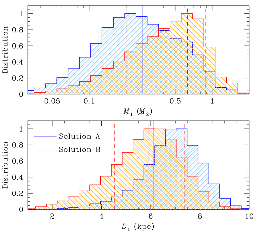
Figure 6.— Posteriors for the primary lens mass, $M_{1}$, and the distance to the lens, $D_{\rm L}$. In each panel, the blue and red distributions are obtained based on the solutions A and B, respectively. For each posterior, the vertical solid line indicates the median and the two dashed lines (together with the line with arrows) represents $1\sigma$ range, estimated by the 16% and 84% of the distribution.

Figure 6 shows the Bayesian posteriors for $M_{1}=M/(1+q)$ (mass of the primary, upper panel) and $D_{\rm L}$ (lower panel). The blue and red curves in each panel are the posteriors corresponding to the solutions A and B, respectively. The estimated masses of the lens components, $M_{1}$ and $M_{2}$, distances, and projected separations between the lens components, $d_{\perp}=sD_{\rm L}\theta_{\rm E}$, for the four degenerate solutions are listed in Table 4. The presented values are the medians of the probability distributions and the uncertainties correspond to 16% and 84% of the distributions. It is found that the primary lens has a mass

$$M_{1}\sim\begin{cases}0.27^{+0.36}_{-0.15}~{}M_{\odot}&\text{for solution A},\\ 0.48^{+0.40}_{-0.28}~{}M_{\odot}&\text{for solution B}.\end{cases}$$ (6)

According to the median values of the individual solutions, the primary lens is a middle (for solution A) and an early (solution B) M dwarf. However, the estimated masses from the two solutions overlap in a wide range because the uncertainties of the mass estimation are substantially bigger than the difference between the masses. See the upper panel of Figure 6. The mass of the lens companion is

$$M_{2}\sim\begin{cases}11^{+16}_{-7}~{}M_{\rm J}&\text{for solution A},\\ 1.3^{+1.1}_{-0.7}~{}M_{\rm J}&\text{for solution B}.\end{cases}$$ (7)

The lens companion has a mass in the planetary regime according to the solution B, while the mass of the companion lies at around the BD/planet boundary according to the solution A. The estimated distance to the lens is

$$D_{\rm L}\sim\begin{cases}7.2^{+1.1}_{-1.3}~{}{\rm kpc}&\text{for solution A},\\ 6.1^{+1.3}_{-1.6}~{}{\rm kpc}&\text{for solution B}.\end{cases}$$ (8)

Similar to the lens mass, the estimated distances from the two solutions overlap in a wide range, as shown in Figure 6. For the solution A, in which the anomaly is produced by a low-mass companion with a binary separation considerably greater or smaller than unity, the projected separation greatly varies depending on the close/wide solution, with $d_{\perp}\sim 0.7$ au for the close solutions and $\sim 4.3$ au for the wide solution. For solution B, in contrast, the difference in the projected separations between the close, $d_{\perp}\sim 2.2$ au, and wide solutions, $\sim 2.8$ au, is relatively small.

6. Resolving Degeneracies

We point out that the degeneracy between the solutions A and B can be lifted from future observations using high-resolution instrument. These observations would enable one to directly measure the relative proper motion by resolving the lens and source, e.g., MACHO LMC-5 (Alcock et al., 2001), OGLE-2005-BLG-169 (Bennett et al., 2015; Batista et al., 2015), OGLE-2005-BLG-071 (Bennett et al., 2020), and MOA-2013-BLG-220 (Vandorou et al., 2019). Then, the degeneracy can be lifted because the two sets of solutions have substantially different values of the relative proper motion: $\mu\sim 4.8~{}{\rm mas}~{}{\rm yr}^{-1}$ for solution A and $\sim 12.1~{}{\rm mas}~{}{\rm yr}^{-1}$ for solution B.

The prospects for early lens-source resolution are more favorable for solution B. This is because the solution yields a substantially higher relative proper motion than the solution A. For OGLE-2005-BLG-169, the lens and source could be resolved from Keck AO observations conducted when the lens-source separation was $\sim 50$ mas (Batista et al., 2015). With the imposition of the same criterion, KMT-2019-BLG-1339L, where “L” denotes the lens, can be resolved from the source if Keck AO observation is conducted $\sim 4.1$ years after the event (in the second half of 2023). Considering that the lens of KMT-2019-BLG-1339, with an expected $H$-band magnitude of $H\sim 20.1$ according to the solution B, is fainter than that of OGLE-2005-BLG-169, with $H\sim 17.9$, the lens resolution would take somewhat longer than $\sim 4.1$ years due to the low signal from the lens. For the solution A, the relative proper motion is much slower. This means that using present instrumentation, one would have to wait 2.5 times longer, perhaps $\gtrsim 11$ years taking account of the fact that the host is somewhat fainter for solution A. However, in either case, the lens can be surely resolved from the source at first light on 30 m class telescopes of the next generation. Once the lens is resolved and its brightness is measured, the degeneracy can be checked using the additional constraint of the lens brightness, which is $H\sim 22.0$ and $H\sim 20.1$ for the solutions A and B, respectively. However, we note that the constraint of the lens brightness is relatively week because the masses and the magnitudes of the lens expected from the two solutions overlap in a wide range. Although future high-resolution followup observations may resolve the degeneracy between the solutions A and B, it will not be possible to resolve the close/wide degeneracy with any existing or proposed instrument.

7. Summary and Conclusion

We carried out an analysis of KMT-2019-BLG-1339, for which a partially covered short-duration anomaly appeared in the light curve. Analysis indicated that the anomaly was generated a low-mass object accompanied to the lens. However, accurate interpretation of the anomaly was prevented by two types of degeneracy, in which one originated from the ambiguity in $\rho$ and the other was the close/wide degeneracy. The former degeneracy, finite-source degeneracy, resulted in ambiguities in both $s$ and $q$, and the latter degeneracy caused ambiguity only in $s$. A Bayesian analysis using the Galactic priors yields that the masses of the lens components were $(M_{1},M_{2})\sim(0.27^{+0.36}_{-0.15}~{}M_{\odot},11^{+16}_{-7}~{}M_{\rm J})$ and $\sim(0.48^{+0.40}_{-0.28}~{}M_{\odot},1.3^{+1.1}_{-0.7}~{}M_{\rm J})$ for the two sets of solutions, indicating that the lens comprises an M dwarf and an Jovian-mass planet or an object near the planet/brown dwarf boundary. We estimated that the lens was located at distances of $D_{\rm L}\sim 7.2^{+1.1}_{-1.3}$ kpc and $\sim 6.1^{+1.3}_{-1.6}$ kpc according to the individual solutions. The finite-source degeneracy can be lifted from future observations using high-resolution instrument because the relative proper motions expected from the degenerate solutions are widely different.

References

- Alard & Lupton (1998) Alard, C., & Lupton, R. H. 1998, ApJ, 503, 325
- Albrow (2017) MichaelDAlbrow/pyDIA: Initial release on github. (Version v1.0.0). Zenodo. http://doi.org/10.5281/zenodo.268049
- Albrow et al. (2009) Albrow, M., Horne, K., Bramich, D. M., et al. 2009, MNRAS, 397, 2099
- Alcock et al. (2001) Alcock, C., Allsman, R. A., Alves, D. R., et al. 2001, Nature, 414,617
- An (2005) An, J. H. 2005, MNRAS, 356, 1409
- Batista et al. (2015) Batista, V., Beaulieu, J.-P., Bennett, D. P., et al. 2015, ApJ, 808, 170
- Bennett et al. (2015) Bennett, D. P., Bhattacharya, A., Anderson, J., et al. 2015, ApJ, 808, 169
- Bennett et al. (2020) Bennett, D. P., Bhattacharya, A., Beaulieu, J.-P., et al. 2020, AJ, 159, 68
- Bensby et al. (2013) Bensby, T., Yee, J. C., Feltzing, S., et al. 2013, A&A, 549, 147
- Bessell & Brett (1988) Bessell, M. S., & Brett, J. M. 1988, PASP, 100, 1134
- Boss et al. (2007) Boss, A. P., Butler, R. P., Hubbard, W. B., et al. 2007, Transactions of the International Astronomical Union, Series A, ed. O. Engvold (Cambridge: Cambridge University Press), 26, 183
- Chabrier (2003) Chabrier, G. 2003, ApJ, 586, L133
- Claret (2000) Claret, A. 2000, A&A, 363, 1081
- Dominik (1999) Dominik, M. 1999, A&A, 349, 108
- Dong et al. (2006) Dong, S., DePoy, D. L., Gaudi, B. S., et al. 2006, ApJ, 642, 842
- Gaudi (1998) Gaudi, B. S. 1998, ApJ, 506, 533
- Gaudi & Han (2004) Gaudi, B. S., & Han, C. 2004, ApJ, 611, 528
- Gould (1992) Gould, A. 1992, ApJ, 392, 442
- Gould (2000) Gould, A. 2000, ApJ, 535, 928
- Griest & Safizadeh (1998) Griest, K., & Safizadeh, N. 1998, ApJ, 500, 37
- Han & Gould (1995) Han, C., & Gould, A. 1995, ApJ, 447, 53
- Han & Gould (2003) Han, C., & Gould, A. 2003, ApJ, 592, 172
- Han et al. (2019) Han, C., Yee, J. C., Udalski, A., et al. 2019, AJ, 158, 102
- Hwang et al. (2013) Hwang, K.-H., Choi, J.-Y., Bond, I. A., et al. 2013, ApJ, 778, 55
- Hwang et al. (2018a) Hwang, K. -H., Kim, H. -W., Kim, D. -J., et al. 2018a, Journal of the Korean Astronomical Society, 51, 197
- Hwang et al. (2018b) Hwang, K.-H., Udalski, A., Shvartzvald, Y., et al. 2018b, AJ, 155, 20
- Kervella et al. (2004) Kervella, P., Thévenin, F., Di Folco, E., & Ségransan, D. 2004, A&A, 426, 29
- Kim et al. (2018) Kim, H.-W., Hwang, K.-H., Shvartzvald, Y., et al. 2018, AAS submitted (arXiv:1806.07545)
- Kim et al. (2016) Kim, S.-L., Lee, C.-U., Park, B.-G., et al. 2016, JKAS, 49, 37
- Mao & Paczyński (1991) Mao, S., & Paczyński, B. 1991, ApJ,374, L37
- Nataf et al. (2013) Nataf, D. M., Gould, A., Fouqué, P., et al. 2013, ApJ, 769, 88
- Shin et al. (2019) Shin, I.-G., Yee, J. C., Gould, A., et al. 2019 AJ, 158, 199
- Skowron et al. (2018) Skowron, J., Ryu, Y.-H., Hwang, K.-H., et al. 2018, Acta Astron.,68, 43
- Tomaney & Crotts (1996) Tomaney, A. B., & Crotts, A. P. S. 1996, AJ, 112, 2872
- Vandorou et al. (2019) Vandorou, A., Bennett, D. P., Beaulieu, J.-P., et al. 2019, submitted (arXiv:1909.04444)
- Udalski et al. (2015) Udalski, A., Szymański, M. K., & Szymański, G. 2015, Acta Astron., 65, 1
- Woźniak (2000) Woźniak, P. R. 2000, Acta Astron., 50, 42
- Yee et al. (2012) Yee, J. C., Shvartzvald, Y., Gal-Yam, A., et al. 2012, ApJ, 755, 102
- Yoo et al. (2004) Yoo, J., DePoy, D. L., Gal-Yam, A., et al. 2004, ApJ, 603, 139