Effects of resolution inhomogeneity in large-eddy simulation

Abstract

Large Eddy Simulation (LES) of turbulence in complex geometries is often conducted using strongly inhomogeneous resolution. The issues associated with resolution inhomogeneity are related to the noncommutativity of the filtering and differentiation operators, which introduces a commutation term into the governing equations. Neglect of this commutation term gives rise to commutation error. While the commutation error is well recognized, it is often ignored in practice. Moreover, the commutation error arising from the implicit part of the filter (i.e., projection onto the underlying discretization) has not been well investigated. Modeling the commutator between numerical projection and differentiation is crucial for correcting errors induced by resolution inhomogeneity in practical LES settings, which typically rely solely on implicit filtering. Here, we employ a multiscale asymptotic analysis to investigate the characteristics of the commutator. This provides a statistical description of the commutator, which can serve as a target for the statistical characteristics of a commutator model. Further, we investigate how commutation error manifests in simulation and demonstrate its impact on the convection of a packet of homogeneous isotropic turbulence through an inhomogeneous grid. A connection is made between the commutation error and the propagation properties of the underlying numerics. A modeling approach for the commutator is proposed that is applicable to LES with filters that include projections to the discrete solution space and that respects the numerical properties of the LES evolution equation. It may also be useful in addressing other LES modeling issues such as discretization error.

I Introduction

The greatest impediment to the use of computer simulation for reliable prediction of many high Reynolds number complex turbulent flows is representing the effects of turbulence. Large Eddy Simulation (LES) has long been considered a promising computationally tractable solution to modeling turbulent flows. However, several challenges of LES modeling must still be addressed before this promise is fulfilled. In particular, LES models are typically formulated under the assumptions of isotropic unresolved turbulence in equilibrium with the large scales, homogeneous isotropic filtering/resolution, and accurate representation of all resolved scales by the underlying numerics. All of these assumptions are typically violated in practice when simulating high Reynolds number complex turbulent flows. In the work reported here, we address the issues that arise from inhomogeneous filtering/resolution. Note that by inhomogeneity of an LES filter or resolution, we mean that the filter or resolution characteristics vary in space; this should not be confused with homogeneity or inhomogeneity of the turbulence.

The challenges posed by resolution inhomogeneity arise because, in this case, the filter that defines the resolved scales does not commute with spatial differentiation. This effect is represented by a commutation term, which should appear in the LES evolution equation. When this effect is neglected it gives rise to commutation error, which was first analyzed in detail by Ghosal and Moin [1]. Since then, several investigators have acknowledged the significant impact commutation error can have on an LES solution [2, 3, 4, 5, 6, 7, 8, 9, 10, 11, 12]. Despite this, the commutation term is often neglected in practice because of the modeling challenges involved. Nevertheless, modeling the commutation term is crucial for developing robust subgrid stress (SGS) models for practical LES applications.

Most of the previous work to address commutation error has been in the context of explicit filtering. Explicit filters, which may be employed in addition to the discrete projection that defines the implicit filter, are used to minimize the effects of numerical discretization errors by defining a filter width larger than the discretization scale [13, 14, 15, 16, 17, 18, 19, 20, 21]. Approximately commuting with differentiation is then viewed as a desirable property of explicit filters to minimize commutation error. In this context, van der Ven [2] introduced a one-parameter family of analytical filters that commute with differentiation up to a given order in filter width. Vasilyev et al. [3] developed a set of constraints for constructing discrete filters that commute with differentiation up to a desired order. Marsden et al. [4] extended the work of [3] to unstructured meshes.

However, in an LES, the projection onto a finite dimensional LES solution space that is inherent in numerical discretization is ultimately responsible for discarding information about the small-scale turbulence [22, 23]. This discrete projection (often referred to as the implicit filter) should therefore be considered as part of the filter. The commutator between filtering and differentiation that arises due to spatially nonuniform numerical discretization and the commutation error that arises from neglecting it are the fundamental issues introduced by resolution inhomogeneity in LES. They are of particular importance in practical LES as many applications rely solely on implicit filtering. Further, the commutation analysis of Ghosal and Moin [1] only applies to smooth formally invertible filters, not filters that include a discrete projection. Similarly, the commutative property of an explicit filter (such as those mentioned above) would only reduce the additional commutation error introduced by the explicit filter applied in addition to the discrete projection. These explicit filters do not represent the commutator associated with the implicit filter and so, in general, do not reduce the corresponding commutation error. Neither the commutation error nor commutator models applicable to implicit filtering have been well investigated and are the focus of this work.

In this paper, we analyze the commutator for filters including discrete projection in Sec. II and explore the impacts of the commutation error in Sec. III. Strategies to model the commutation term are explored in Sec. IV, and conclusions are offered in Sec. V.

II Analysis of the Inhomogeneous Commutator

To define the large scales of turbulence to be simulated in an LES, we define a filter operator $\mathcal{F}$ which maps turbulent fields to large-scale (LES) fields. If $\mathcal{F}$ is shift invariant (commutes with arbitrary shift operators), then the filter is said to be homogeneous and it commutes with derivative operators. To define the large scales, $\mathcal{F}$ should be smoothing, but to enable solution on a computer, we will also insist that the range of $\mathcal{F}$ be finite dimensional, thereby including the discretization for numerical solution. Thus, as discussed above, $\mathcal{F}$ includes what is commonly called the implicit filter (projection onto the discretization) in addition to any explicit filter that may be employed. Unless the discretization is a Fourier truncation, such a filter is not homogeneous. Instead, it may be “discretely homogeneous,” that is, invariant to spatial shifts by integral multiples of a discretization scale $\Delta$. For example, projections to finite volume, finite element and spline solution spaces on uniform grids are discretely homogeneous, while the same projections on nonuniform grids are discretely inhomogeneous (see [24]). The consequences of such resolution inhomogeneity are the subject of the current paper. Resolution inhomogeneity is a property of the filter, and should not be confused with inhomogeneity of turbulence, which refers to turbulence whose statistics are not invariant to spatial shifts.

Assuming that mean quantities in an LES are well resolved, the filtered fluctuating Navier-Stokes momentum equations read

$$\frac{\partial\overline{u^{\prime}_{i}}}{\partial t}+U_{j}\overline{\frac{\partial u^{\prime}_{i}}{\partial x_{j}}}+\overline{\frac{\partial u^{\prime}_{i}u^{\prime}_{j}}{\partial x_{j}}}-\frac{\partial\langle u^{\prime}_{i}u^{\prime}_{j}\rangle}{\partial x_{j}}=-\overline{\frac{\partial p^{\prime}}{\partial x_{i}}}+\nu\overline{\frac{\partial^{2}u^{\prime}_{i}}{\partial x_{j}\partial x_{j}}},$$ (1)

where over-line represent filtering, that is $\overline{\cdot}=\mathcal{F}(\cdot)$, $\langle\cdot\rangle$ represents the mean or expected value, $U_{i}$ is the mean velocity, and $u^{\prime}_{i}$ and $p^{\prime}$ are the fluctuating velocity and pressure respectively. To obtain the fluctuating LES equations, one would like to interchange the order of filtering and spatial differentiation, but with inhomogeneous filters, this would introduce commutation error for each of the filtered derivative terms in (1). These errors would be small for the viscous term and the errors in the pressure term would be subsumed in the treatment of continuity. The remaining terms representing convection by the mean and the fluctuations are thus of primary interest here. In many turbulent flows the mean velocity relative to the grid is much larger than the fluctuating velocity, so arguably the commutation error for the mean convection term is most important. Further, there are numerous other issues associated with modeling $\overline{u^{\prime}_{i}u^{\prime}_{j}}$ in the fluctuating convection term, including modeling the subgrid stress and filtering the nonlinear products used in the modeling [18]. For these reasons, we are particularly focused on the effects of resolution inhomogeneity on the mean convection term $U_{j}\overline{\partial u^{\prime}_{i}/\partial x_{j}}$ here, although the results may be insightful for the nonlinear term as well.

For the purposes of analysis, it is useful to further simplify the mean convection and consider the effects of the resolution inhomogeneity on the filtered one-dimensional advection equation:

$$\overline{\frac{\partial u}{\partial t}+U\frac{\partial u}{\partial x}}=0,$$ (2)

where $U$ is the constant convection velocity. Furthermore, let $\delta/\delta x$ denote a discrete derivative operator defined on the discrete solution space. Then (2) can be written as

$$\frac{\partial\overline{u}}{\partial t}+U\frac{\delta\bar{u}}{\delta x}=-U\mathscr{C}(u),$$ (3)

where $\mathscr{C}(u)=\overline{\partial u/\partial x}-\delta\overline{u}/\delta x$ is the commutation term (similar to a commutator). The commutation term $\mathscr{C}(u)$ can be decomposed into an inhomogeneous and homogeneous part as $\mathscr{C}(u)=\mathscr{C}^{I}(u)+\mathscr{C}^{H}(u)$ where,

$$\mathscr{C}^{I}(u)=\overline{\frac{\partial u}{\partial x}}-\overline{\frac{\partial{u}}{\partial\xi}}\frac{d\xi}{dx}\qquad\mathscr{C}^{H}(u)=\overline{\frac{\partial{u}}{\partial\xi}}\frac{d\xi}{dx}-\frac{\delta\overline{u}}{\delta x},$$ (4)

and $\xi$ is the new spatial coordinate in which the grid or resolution is uniform as in [1]. The homogeneous part represents the effects of the numerical discretization error in $\delta/\delta x$ and is non-zero even if the resolution is homogeneous. The inhomogeneous part characterizes the effects of the inhomogeneous resolution and is zero when the resolution is homogeneous. This formulation can be extended to three dimensions as well as to the full Navier-Stokes equations [24]. However, for the nonlinear terms in the Navier-Stokes equations there is an additional complication in the definition of the discrete derivative operator [18], which impacts the definition of the commutator [24].

There is also a subtlety to this decomposition when the filter is discretely homogeneous in $\xi$ since discretely homogeneous filters can be decomposed into a homogeneous filter followed by sampling on a uniform grid. If the homogeneous filter is defined to include a Fourier cutoff with cutoff wavenumber less than the Nyquist wavenumber for the grid, the sampling does not discard information, and this is usually what is intended when defining the filter. When applying this to the decomposition (4), we can choose to include the effect of sampling as part of $\mathscr{C}^{I}$ or $\mathscr{C}^{H}$. Here, we will generally choose the latter, so that $\mathscr{C}^{I}$ is expressed in terms of a non-invertible homogeneous filter in $\xi$.

In numerical analysis one generally aspires to make the resolution sufficiently fine so that $\mathscr{C}^{H}$ is negligible, but an LES is by definition under resolved and so $\mathscr{C}^{H}$ generally needs to be considered. Models for $\mathscr{C}^{H}$ are not available, so it is often neglected leading to discretization error [15, 16, 17]. Although discretization error is widely acknowledged by LES practitioners, the inhomogeneous term $\mathscr{C}^{I}$ has received less attention. The effects of neglecting $\mathscr{C}^{I}$, as well as modeling strategies for $\mathscr{C}^{I}$, are not well understood and are the primary focus of the current paper.

II.1 Asymptotic Analysis of the Inhomogeneous Commutator

In the seminal work of Ghosal and Moin [1], the commutator is estimated through Taylor series analysis allowing the commutator to be analyzed. However there were limitations of that work. First, the analysis uses an approximate inversion of the filter operator, and as such is formally only applicable to invertible filters, and thus not to filters including discrete projections as considered here. And second, in simplifying the expansions, an ad hoc ordering is employed which resulted in the neglect of terms that a more careful analysis would identify as important. Here we pursue a similar program using asymptotic analysis with the goals of placing the results of Ghosal and Moin [1] for invertible filters on firmer ground (Sec. II.1.1), and of developing statistical characterizations of the commutator applicable to non-invertible filters (Sec. II.1.2). The results for invertible filters are of interest here because they can provide guidance on appropriate forms and dependencies for a model of the commutator. This may be valuable because filters that include discrete projections can be considered to be limits of sequences of invertible filters.

II.1.1 Series Representation of the Inhomogeneous Commutator

While Ghosal and Moin [1] employ an ad hoc ordering, their results can be consistently interpreted asymptotically. As described in Appendix A.1, the analysis in [1] employs a mapping of the physical space $x$ to a mapped space $\xi$ in which the resolution is uniform to define the filtering operator. A Taylor series expansion yields a series representations for $\mathscr{C}^{I}$ that is valid asymptotically for $\Delta_{\xi}\rightarrow 0$, where $\Delta_{\xi}$ is the uniform resolution in $\xi$ space. This expansion is in terms of the derivatives of the unfiltered field $u$. To express the commutator in terms of the derivatives of $\overline{u}$, the filter is inverted through another asymptotic expansion in $\Delta_{\xi}$. But, to properly order the expansion, the way in which the derivatives of $\overline{u}$ scale with $\Delta_{\xi}$ must be determined. In Ghosal and Moin [1], it is assumed that $u=e^{i\kappa x}$ and their analysis is consistent with the assumption that $\kappa\sim\Delta_{\xi}^{-p}$ for $0<p<1$ (see Appendix B). However, this is not necessarily consistent with the way the derivatives of $\overline{u}$ scale when $u$ is the turbulent velocity.

Assuming the resolution in physical space $\Delta(x)$ is in the inertial range of a high Reynolds number turbulence, the Kolmogorov hypotheses imply that

$$\frac{\partial^{n}\overline{u}}{\partial x^{n}}\sim\Delta_{\xi}^{1/3-n}$$ (5)

(see Appendix A.1). With this ordering, the lowest order expansion for the commutator is given by

$$\begin{split}\mathscr{C}^{I}(u)&=-M_{2}\Delta\frac{d\Delta}{dx}\frac{\partial^{2}\overline{u}}{\partial{x}^{2}}+\left(\frac{M_{2}^{2}}{2}-\frac{M_{4}}{6}\right)\Delta^{3}\frac{d\Delta}{dx}\frac{\partial^{4}\overline{u}}{\partial{x}^{4}}+\dots+C_{N}\Delta^{N-1}\frac{d\Delta}{dx}\frac{\partial^{N}\overline{u}}{\partial{x}^{N}}+\dots+\mathcal{O}(\Delta_{\xi}^{4/3})\\ &=\frac{d\Delta}{dx}\sum_{n=1}^{\infty}C_{2n}\Delta^{2n-1}\frac{\partial^{2n}\overline{u}}{\partial{x}^{2n}}+\mathcal{O}(\Delta_{\xi}^{4/3})\end{split},$$ (6)

where $M_{k}$ is the $k^{\rm th}$ order moment of the filter kernel, $N$ is even, and in general, the coefficient $C_{j}$ on the $j^{th}$ order term depends on the moments of the filter up to order $j$. In Ghosal and Moin [1], only the first term in this series is retained because the other terms are higher order in $\kappa\Delta\sim\Delta_{\xi}^{1-p}$, but clearly this would not be consistent with filtering turbulence in a Kolmogorov inertial range as (6) is.

An alternative approach to developing a series representation of $\mathscr{C}^{I}$ is formulated for a different, though related asymptotic limit. Consider the situation in which the derivative $d\Delta/dx$ is order $\epsilon$, where $\epsilon$ is asymptotically small. In this case, a multiscale asymptotic analysis of $\overline{u}$ in terms of a fast variable $\tilde{x}$ and slow variable $w=\epsilon x$ yields the simple result $\mathscr{C}^{I}=-\epsilon\partial\overline{u}/\partial w+\mathcal{O}(\epsilon^{2})$ (see Appendix A), which can be expressed directly as a convolution operator applied to the unfiltered field, where the kernel is in terms of the filter kernel and its derivative (31). As with the analysis discussed above, a Taylor series representation of the filter inverse can be applied to produce a series representation of the commutator in terms of the filtered field and its derivatives. However, the asymptotic interpretation may be different. In particular, the $\epsilon\rightarrow 0$ limit can be approached by allowing the length scale $L_{\Delta}$ over which the resolution changes ($\frac{1}{L_{\Delta}}\sim\frac{1}{\Delta}\frac{d\Delta}{dx}$) to grow while $\Delta$ remains constant. In this case derivatives of $\overline{u}$ as well as $\Delta$ are order one in $\epsilon$. Alternatively, $L_{\Delta}$ can remain constant while $\Delta$ goes to zero, which is equivalent to the previous analysis. In this case, $\Delta\sim\epsilon$ and for inertial range turbulence, the $n^{th}$ derivative of $\overline{u}$ scales as $\epsilon^{1/3-n}$. In either case, one obtains

$$\begin{split}\mathscr{C}^{I}(u)=\frac{d\Delta}{dx}\sum_{n=1}^{\infty}C_{2n}\Delta^{2n-1}\frac{\partial^{2n}\overline{u}}{\partial\tilde{x}^{2n}}+\mathcal{O}(\epsilon^{q})\end{split},$$ (7)

where $q=2$ when the asymptotic limit is taken with constant $\Delta$ while $q=4/3$ when it is taken at constant $L_{\Delta}$ (see Appendix A.1). This is the same series as in (6).

Despite the fact that the above analyses are predicated on the use of an invertible filter and we are concerned with filters that include a discrete projection, the characteristics of the commutator expression provide insights relevant to modeling of the commutation term. First, note that to leading order this approximation is proportional to $d\Delta/dx$, and is a series in the even $x$ derivatives of $\bar{u}$. The lowest order term appears as a viscous term, which is dissipative when $d\Delta/dx>0$ (i.e. convecting from fine to coarse resolution), and the higher order terms are hyperviscous. Similarly, these terms would be anti-dissipative when convecting from coarse to fine resolution, and thus will create resolved energy in this case. Clearly this commutator expression is characterizing the transfer of energy between resolved and unresolved scales as a consequence of the resolution inhomogeneity. In addition, since each of the terms in (6) and (7) are of the same asymptotic order, they are all equally important, and indeed, depending on the characteristics of the filter, the higher order derivative terms could dominate. This suggests that a model of the commutator formulated as a differential operator should include as high-order derivatives as possible. It is also interesting to observe that the asymptotically higher order terms include dispersive terms in addition to dissipative ones, and that higher order derivatives of $\Delta$ appear (see Appendix B).

Finally, this analysis may provide clarity on some of the existing literature surrounding commutation error. In particular, the deconvolution analysis in [1] has often been used to motivate the development of smooth explicit filters whose first $N-1$ moments are zero so that the commutation error is of explicit order $\Delta^{N}$ (e.g, [3, 4, 2, 5]). However, this is only meaningful if the derivatives of $\overline{u}$ scale sufficiently weakly with $\Delta$, as discussed above, so that the first terms in (6) dominate asymptotically. Unfortunately, for high Reynolds number turbulence, each term in (6) is of the same asymptotic order. Therefore, this analysis suggests that constructing filters so that the coefficients $C_{j}$ for $j<N-1$ in (6) vanish would likely not render the commutator negligible. The commutator will thus need to be modeled.

II.1.2 Statistical Analysis of the Inhomogeneous Commutator

Because an LES filter always includes a projection to the finite-dimensional numerical solution space, either explicitly or implicitly, the information in a filtered turbulent field is not sufficient to determine the evolution of that filtered turbulence [25]. As a consequence, one can only expect LES models, including models of the commutator, to match statistical characteristics of the quantity being modeled [24]. The challenge lies in identifying the important statistical characteristics and developing models capable of representing them. Here we analyze a priori statistical properties of the commutator in terms of statistical characteristics of the unfiltered turbulence, to inform potential commutator models.

The finite-dimensional projection inherent to LES filters determines the information available in an LES upon which to base a model, and so a deconvolution analysis is ill-suited to determining statistical properties. Instead, we apply the multiscale asymptotic analysis discussed in Sec. II.1.1 and detailed in Appendix A.1 to characterize the statistics of the commutator. In Appendix A.2, such an analysis is applied to an inhomogeneous three-dimensional isotropic filter characterized by a slowly varying filter width $\Delta$. After performing a Fourier transform in the fast variable for which the filter is homogeneous, the commutator between filtering and differentiation applied to turbulent velocity fluctuations $u_{j}$ can be written explicitly as

$$\widehat{\mathscr{C}_{i}^{I}}(u_{j})=-\frac{\partial\Delta}{\partial x_{i}}\widehat{G}^{\prime}(\Delta|\boldsymbol{\kappa}|)|\boldsymbol{\kappa}|\widehat{u}_{j}(\boldsymbol{\kappa}),$$ (8)

where $\boldsymbol{\kappa}$ is the wavenumber vector, $\widehat{G}$ is the Fourier transform of the isotropic filter kernel $G$, and $\widehat{G}^{\prime}$ is the derivative of $\widehat{G}$ with respect to its argument. Note that the “local Fourier transform” analysis in [26] holds in this multiscale asymptotic sense.

The commutator is a linear operator, and (8) shows that it is proportional to the gradient of $\Delta$ and its spectrum is proportional to $\widehat{G}^{\prime}$. The commutator thus acts on the wavenumbers over which the filter spectrum rolls off from order one to zero. These are generally the smallest resolved scales of the LES. For a Fourier cutoff filter in which $\widehat{G}$ is discontinuous at the cutoff wavenumber $\kappa_{c}$, $\widehat{G}^{\prime}$ is a Dirac delta function at $\kappa_{c}$, so in this case the commutator acts only at the slowly varying cutoff.

While (8) is an explicit expression for the commutator, it requires knowledge of the unfiltered quantity, which is generally not available. If the turbulence is being convected by a mean velocity $U_{i}$, then the commutator $\mathscr{C}_{i}^{I}(u_{j})$ arising from the mean convection term enters the $u_{j}$ evolution equation as $U_{i}\mathscr{C}_{i}^{I}(u_{j})$, and (8) can be used to determine the contribution of the commutator to the evolution of the filtered spectrum tensor, and in particular the three-dimensional filtered energy spectrum $\overline{E}(\mathbf{w},\kappa)$, to obtain

$$\tilde{\mathscr{C}}^{I}(\overline{E})=-U_{k}\frac{\partial\Delta}{\partial x_{k}}\widehat{G}(\Delta\kappa)\widehat{G}^{\prime}(\Delta\kappa)\kappa E(\kappa)\\$$ (9)

where $\tilde{\mathscr{C}}$ indicates the contribution of the commutator to the evolution equation for its argument. This contribution still requires knowledge of the unfiltered turbulence, in this case the unfiltered spectrum, but at least in high Reynolds number isotropic turbulence, Kolmogorov inertial range theory provides a good model for $E$. This is useful because a priori consistency of a commutator model with (9) is a necessary condition for LES prediction of the energy spectrum [27, 24]. Similarly, integrating (9) over $\kappa$ yields the contribution of the commutator to the evolution of the resolved turbulent kinetic energy $k^{>}$, and a necessary condition for LES prediction of $k^{>}$. For the special case of a Fourier cutoff filter, the result simplifies to

$$\tilde{\mathscr{C}}^{I}(k^{>})=U_{k}\frac{\partial\kappa_{c}}{\partial x_{k}}E(\kappa_{c}),$$ (10)

which is consistent with the result obtained by Moser et al. [24] by other means. For coarsening resolution ($U_{k}\partial\kappa_{c}/\partial x_{k}<0$), the commutator transfers energy to unresolved scales with the dissipation occurring only at the cutoff wavenumber. Similarly, for refining resolution ($U_{k}\partial\kappa_{c}/\partial x_{k}>0$), the commutator transfers energy from the subgrid to the resolved turbulence at the cutoff wavenumber. Further, when this spectral analysis is applied to the full nonlinear terms in the filtered Navier-Stokes equations, an additional commutator contributes to the evolution of the spectrum tensor, which can be determined in terms of $\widehat{S}_{ijk}(\boldsymbol{\kappa})$, the Fourier transform of the two-point third-order correlation tensor.

II.2 Numerical Analysis of Commutation Error

When convecting through a coarsening grid, the resolved fluctuations in a fine region will be moving into a coarse region in which not all the resolved scales can be represented. Similarly, solution scales that cannot be resolved in a coarse region will become resolvable as the solution convects into a finer resolution region. The previous subsections show how the inhomogeneous commutator $\mathscr{C}^{I}$ is responsible for transferring energy between the subgrid and resolved turbulence in both these cases. However, notice that the injection of energy into the resolved scales is required for the refining resolution case to maintain consistency with the definition of the filter, but that neglecting this effect will not lead to numerical inconsistencies since the coarse region solution is perfectly well represented in the fine region. This is not true for flow through a coarsening grid. For this reason, our investigation of commutation error (neglect of $\mathscr{C}$) in this paper is particularly focused on flow through coarsening grids because of the numerical consistency issues inherent to this case.

The impact of the commutator and specifically its neglect is affected by the characteristics of the discrete derivative operator, which is accounted for in the homogeneous commutator $\mathscr{C}^{H}$. Here, by recalling results from numerical analysis [28, 29, 30, 31, 32, 33, 34, 35], we consider the impact of neglecting both commutators, as is typical in LES, in the case of a filter consisting of just the projection to the finite-dimensional discrete solution space (i.e. only an implicit filter). Neglecting the commutator in (3) gives:

$${\frac{\partial\overline{u}}{\partial t}+U\frac{\delta\overline{u}}{\delta x}}=0.$$ (11)

We begin by recalling, as an example, the solution of (11) using a second-order centered finite difference scheme on a uniform mesh with mesh size $\Delta$. The numerical first derivative is then given by $\delta u_{j}/\delta x=\tfrac{1}{2\Delta}(u_{j+1}-u_{j-1})$.

It is well recognized that, for initial conditions of the form $e^{i\kappa x}$, solutions of (11) take the form $e^{i(\kappa x-\omega t)}$ and propagate at a phase velocity that depends on their wavenumber [28]. The relation $\omega=\omega(\kappa)$ is called the dispersion relation. Individual waves propagate at a phase speed given by $c(\kappa)=\omega(\kappa)/\kappa$; however, the evolution of a wave packet, which can be decomposed into Fourier modes with wavenumbers ranging over a relatively narrow band, is governed by the group velocity:

$$\mathcal{G}(\kappa)=\frac{d\omega}{d\kappa}(\kappa).$$ (12)

The group velocity is the velocity at which information and energy propagate and as such is of great importance in LES.

Substituting the form $u_{j}=e^{i(\kappa x_{j}-\omega t)}$ into (11) with the second order centered difference scheme yields the dispersion relation and group velocity:

$$\omega(\kappa)=U\kappa^{\prime}(\kappa)=U\frac{\sin(\kappa\Delta)}{\Delta}\qquad\mbox{and}\qquad\mathcal{G}(\kappa)=U\cos(\kappa\Delta),$$ (13)

where $\kappa^{\prime}$ is the spectrum of the numerical derivative operator, which is often referred to as the effective (or modified) wavenumber. Notice that at the Nyquist wavenumber for the grid, $\kappa_{c}=\pi/\Delta$, both $\kappa^{\prime}$ and $\omega$ are zero. As a consequence there is a wavenumber $\kappa_{a}\in(0,\kappa_{c})$ at which $\omega$ is maximized with value $\omega_{\text{max}}(\Delta)=\omega(\kappa_{a})$ ($\kappa_{a}=\kappa_{c}/2$ for second order central difference) so that the group velocity is zero. Therefore, for $\kappa\in(\kappa_{a},\kappa_{c})$ the group velocity is negative so that wave packets with wavenumbers in this range will propagate upstream against the convection velocity. Also note that for any frequency $\omega<\omega_{\text{max}}(\Delta)$, there are two wavenumbers that will evolve with that frequency, one with positive and one with negative group velocity. The wavenumber with positive group velocity ($\kappa<\kappa_{a}$) is a consistent approximation to a solution of the advection equation while the other ($\kappa>\kappa_{a}$) is spurious. As pointed out by Vichnevetsky [29], a general solution to (11) can therefore be decomposed as $u=p+q$, where $p$ has a forward propagation and is a consistent approximation, and $q$ propagates backwards and is spurious.

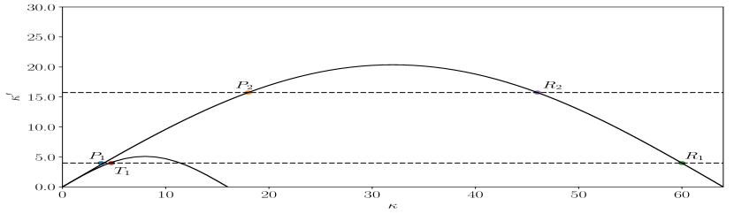
(a)

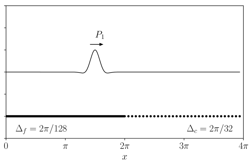
(b)

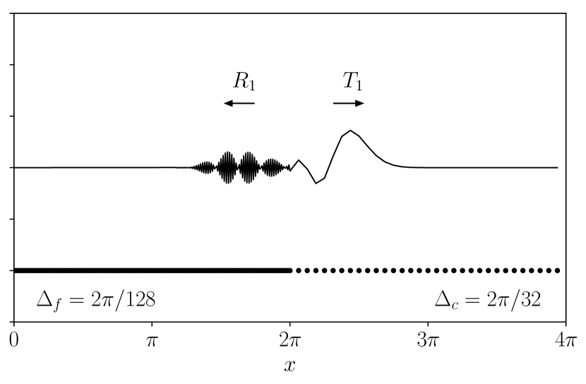
(c)

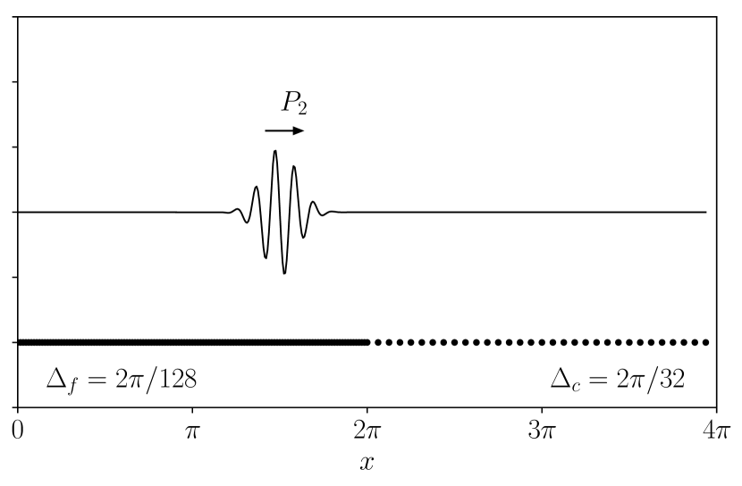
(d)

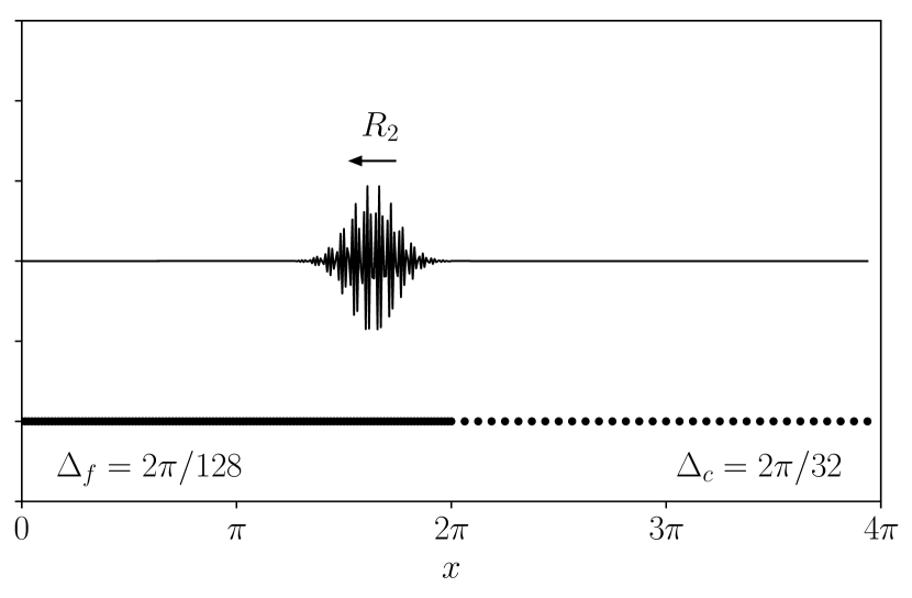
(e)

Figure 1: (a) The second order centered difference dispersion relation for both the fine ($\Delta_{f}=2\pi/128$) and coarse ($\Delta_{c}=2\pi/32$) regions of the grid, (b) An incident wave $P_{1}$ ($\bullet$) that can be resolved in both the fine and coarse regions. (c) The subsequent reflected wave $R_{1}$ ($\bullet$) and transmitted wave $T_{1}$ ($\bullet$) after the $P_{1}$ wave has propagated through the resolution change. (d) An incident wave $P_{2}$ ($\bullet$) that can only be resolved in the fine region. (e) The subsequent reflected wave $R_{2}$ ($\bullet$) after the $P_{2}$ wave has propagated through the resolution change.

Consider next a grid for a domain of length $L=4\pi$ with a sharp change in resolution from $\Delta_{f}=2\pi/128$ to $\Delta_{c}=2\pi/32$ as shown in Fig. 1, and two different initial conditions given by

$$u_{i}(x,t=0)=\cos(\eta_{i}x)e^{-5(x-3\pi/2)^{2}},$$ (14)

with $\eta_{1}=4$ and $\eta_{2}=18$, which we refer to as wave packets $P_{1}$ and $P_{2}$, respectively. The energy spectrum of these wave packets is the sum of three Gaussian functions of wavenumber, with standard deviation of $\sqrt{5}$. They are centered around $\kappa=\pm\eta_{i}$ and 0. As a consequence, more than 99% of the energy resides in wavenumbers with $|\kappa|<\eta+5.8$. In the fine region, $\kappa^{f}_{a}=32$, so both wave packets have virtually all of their energy in wavenumbers $|\kappa|<\kappa^{f}_{a}$. Both wave packets are thus well resolved in the fine region and propagate as expected with approximately the convection velocity (Figs. 1(b) and 1(d)). The packet $P_{1}$ is centered around the wavenumber $\kappa=4$ which can be supported on the coarse as well as the fine grid (Fig. 1(a)), with more than 90% of the energy residing in wavenumbers with $|\kappa|<\kappa^{c}_{a}=8$. The packet therefore mostly propagates into the coarse region (Fig. 1(c)) in a wave packet centered around a slightly larger wavenumber with a slightly lower group velocity ($T_{1}$ in Fig. 1(a)). But because of the resolution change, some of $P_{1}$ is also reflected back into the fine region in a wave packet centered around a much higher wavenumber ($R_{1}$ in Fig. 1(a)) which has negative group velocity. Since (11) with a central difference derivative scheme is an energy preserving approximation of the advection equation, the energy from the incident wave is split between the reflected wave and the transmitted wave [29, 30, 31, 32]. The $P_{2}$ packet is centered around the wavenumber $\kappa=18$ on the fine grid, which cannot be supported on the coarse grid ($P_{2}$ in Fig. 1(a)), and indeed virtually none of the energy resides in wavenumbers with $|\kappa|<\kappa^{c}_{a}$. It therefore cannot propagate into the coarse region and instead is entirely reflected back into the fine region (Fig. 1(e)) in a packet centered around a much larger wavenumber ($R_{2}$ in Fig. 1(a)). In both cases, it is effective wavenumbers that are preserved through the resolution change (Fig. 1(a)). The reflected waves $R_{1}$ and $R_{2}$ are entirely spurious.

Because the system is linear, the above results can be extended to grids with gradually changing resolution. In this case, a local wavenumber $\kappa_{j}$ and a local group velocity $\mathcal{G}_{j}$ can be defined by substituting a given frequency $\omega$ (or $\kappa^{\prime}$) and the local grid spacing $\Delta(x_{j})$ into (13). As above, there will be two possible values of $\kappa_{j}$, $\kappa_{j}^{(1)}$ and $\kappa_{j}^{(2)}$, satisfying $\kappa_{j}^{(1)}<\kappa_{j}^{(2)}$ and $(\kappa^{(2)}_{j}\Delta(x_{j}))=\pi-(\kappa_{j}^{(1)}\Delta(x_{j}))$, with group velocities $G_{j}$ and $-G_{j}$, respectively. There are three main results of such an analysis [33, 32] that will be relevant for our purposes. First, no reflections occur if the local group velocity is uniform and nonzero, as expected. Second, a total reflection occurs for all wavenumbers that become unresolvable on the grid (i.e., exceed the Nyquist wavenumber), and the reflection occurs at the point where the local group velocity vanishes ($\mathcal{G}_{j}=0$). Thirdly, no reflections occur for wavenumbers that can be resolved throughout the domain if $\Delta(x_{j})$ varies over length scales that are long compared to the wavelength $\lambda=2\pi/\kappa_{j}$ ($\frac{\lambda}{\Delta}\frac{d\Delta}{dx}\ll 1$). Thus, wave packets analogous to $P_{1}$ will be completely transmitted through a sufficiently smooth resolution change.

The behavior described here is representative of all energy-conserving numerical schemes with two wavenumbers per effective wavenumber. These are among the most common numerical schemes used in turbulence applications (e.g., centered difference, B-splines, finite volume), however, other numerics with different propagation properties are possible. For instance, consider the box scheme whose semi-discretization of (11) is given by

$$\frac{\partial}{\partial t}\left(\frac{u_{j}+u_{j+1}}{2}\right)+U\frac{u_{j+1}-u_{j}}{x_{j+1}-x_{j}}=0,$$ (15)

which is also energy preserving. Instead of reflecting unresolvable scales of motion at higher wavenumbers into the fine region, the box scheme transmits unresolvable scales at lower wavenumbers through the coarse region (similar to an aliasing effect) [34, 35]. The result is still spurious numerical oscillations. These results from numerical analysis have profound consequences for LES. When LES turbulence convects into a more coarsely resolved region, the spectral characteristics of the numerical derivative operator $\delta/\delta x$ dictate that neglecting the inhomogeneous commutator can produce non-physical fine-scale noise propagating upstream, spoiling the solution far from the resolution change. This is explored in the next section.

III Impacts of Resolution Inhomogeneity on LES

The commutator analysis of Sec. II indicates that the combined effects of neglecting the inhomogeneous commutator and the dispersion characteristics of the numerical derivative operator could have a profound impact on an LES of turbulence flowing through a domain with varying spatial resolution. To characterize this impact, we consider a simple case of such a flow, making two simplifications to clearly expose the effects. As discussed in Sec. II, we consider commutation error for mean convection since this is commonly the dominant effect. This is consistent with the Taylor frozen field hypothesis. Moreover, a localized packet of turbulent fluctuations is used to expose the non-local effects of commutation error. Again we consider filters that consist of only an implicit projection to the discrete solution space.

III.1 A Numerical Experiment

Under the frozen field hypothesis and neglecting commutators, the LES equations for turbulence flowing at constant velocity $U_{x}$ in the $x$ direction simplify to:

$$\frac{\partial\overline{\mathbf{u}^{\prime}}}{\partial t}+U_{x}\frac{\delta\overline{\mathbf{u}^{\prime}}}{\delta x}=0.$$ (16)

The resolution in the $x$ direction is made to vary with $x$, while the resolution in the other directions is constant, and periodic boundary conditions are imposed in all three directions. The filter is defined as a projection onto a periodic B-spline representation in the $x$-direction and Fourier spectral representations in the $y$- and $z$-directions. The $\delta/\delta x$ operator in (16) is defined as B-spline collocation. B-spline collocation is a convenient numerical treatment for inhomogeneous resolution offering a range of orders of accuracy, and have been advocated for use in turbulence simulations [17, 36, 37, 38, 39, 40]. Let $B_{n}^{k}$ denote the $n$th derivative B-spline operator of order $k$, and $B_{n}^{CD}$ denote the $n$th derivative second-order centered difference operator. The spectra of the $B_{1}^{k}$ operators (Fig. 2) have similar propagation properties as the $B_{1}^{CD}$ operator discussed in Sec. II.2, in that there are generally two wavenumbers $\kappa$ that have the same effective wavenumber $\kappa^{\prime}$, one with positive group velocity and the other with negative group velocity. Further, with increasing $\kappa$, the negative group velocities get larger in magnitude (larger negative slopes on the right side of Fig. 2(a)).

For the results presented here, a third-order low storage Runge-Kutta method is used for time advancement [41]. Note that the spurious reflection/transmission phenomena described in Sec. II.2 depend only on spatial discretization [42].

A two dimensional slice of the numerical grid is shown in Fig. 3a. The domain in the propagation direction is divided into a uniform fine region of size $2\pi$, a uniform coarse region of size $6\pi$, and two transition regions of approximate size $2\pi$ in which the resolution is inhomogeneous. The fine resolution spacing between B-spline knot points is $\Delta_{f}=2\pi/128$, and the coarse knot spacing is $\Delta_{c}=2\pi/32$. In the transition regions, the knot spacing is designed to vary as a Sigmoid function between $\Delta_{f}$ and $\Delta_{c}$ over a distance in $x$ of order $1/\alpha$. To this end, the mapping function $g(\xi):[0,1]\to[x_{{\rm start}},x_{\rm end}]$ is defined implicitly through the differential equation:

$$\Delta(x)\equiv\frac{dg(\xi)}{d\xi}\Delta_{\xi}=\frac{\Delta_{f}}{1+e^{\alpha g(\xi)}}+\frac{\Delta_{c}}{1+e^{-\alpha g(\xi)}},$$ (17)

where, $\Delta_{\xi}=1/N_{\xi}$ is the uniform resolution in $\xi\in[0,1]$, with $N_{\xi}$ the number of knot intervals in the transition region. The knot points $x_{j}$ are then defined as $x_{j}=g(j\Delta_{\xi})$ for $j=0,1,\ldots N_{\xi}$. The parameter $\alpha$ controls the sharpness of the grid change, with the transition thickness defined by $(\Delta_{c}-\Delta_{f})/(d\Delta/dx)=4/\alpha$. To generate the knot points used here, (17) was solved numerically for $g(\xi)$ using a standard Runge–Kutta–Fehlberg method and $g(0)=x_{\rm start}=-\pi$, $\alpha=4$ and $N_{\xi}=75$. With these parameters, $g(1)\approx 3.1996$, defining a transition region grid on an interval slightly larger than $2\pi$.

The domain in the two spectral directions is $[0,2\pi]$ and with an effective uniform grid spacing of $\Delta_{f}$. Thus, LES turbulence will be convected through an anisotropic, inhomogeneous grid — a common scenario in practice for structured grids. Moreover, in this configuration the three dimensional commutation error simplifies to the one dimensional case, which will expose the implications of the numerical analysis in Section II.2 for commutation error in LES.

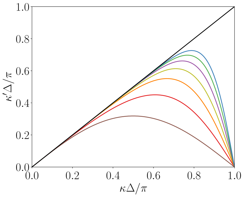
(a)

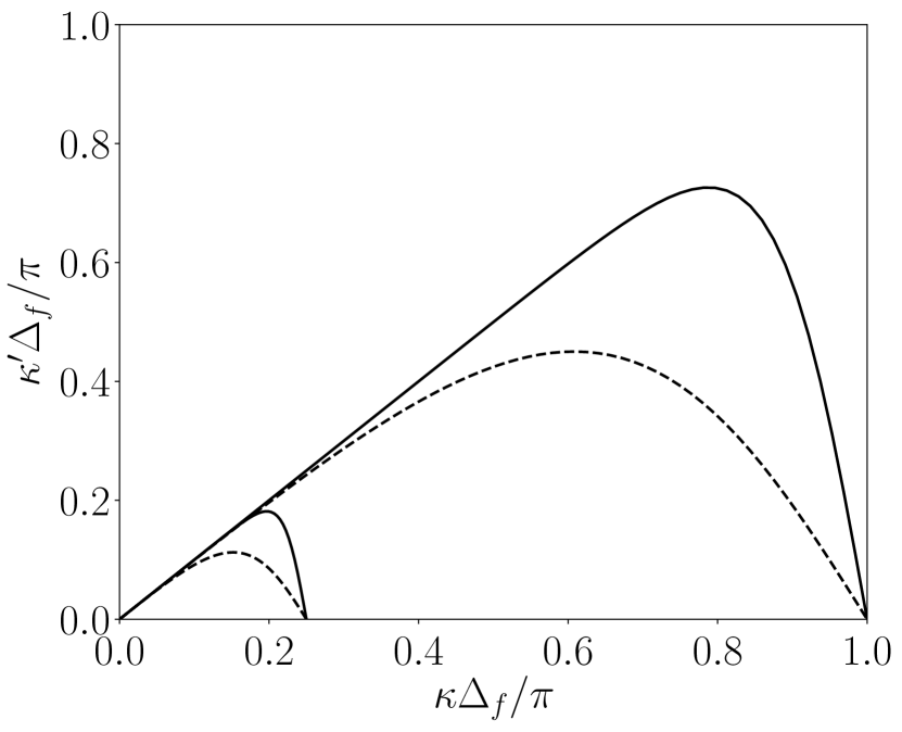
(b)

Figure 2: (a) The spectrum of the first derivative operators for a B-spline collocation method of several orders, a second-order centered difference method, and a spectral method;   ($B_{1}^{2}$),   ($B_{1}^{3}$),   ($B_{1}^{4}$),   ($B_{1}^{5}$),   ($B_{1}^{6}$),   ($B_{1}^{7}$),   ($B_{1}^{CD}$),   (Spectral). (b) The consistently normalized spectrum of the $B_{1}^{2}$ and $B_{1}^{7}$ operators for the fine region of the domain with spacing $\Delta_{f}$ and the coarse region of the domain with spacing $\Delta_{c}=4\Delta_{f}$;   ($B_{1}^{7}$),       ($B_{1}^{2}$).

The initial condition is taken to be a ‘packet’ of well-resolved, homogeneous, isotropic turbulence. This packet is analogous to the wave packets studied in the one-dimensional examples in Sec. II.2. To create this packet, a spectral LES of infinite Reynolds number homogeneous, isotropic turbulence was performed in a $2\pi\times 2\pi\times 2\pi$ domain with 64 Fourier modes in each direction. A Smagorinsky model was used to represent the subgrid stress in this simulation and a negative viscosity forcing that isotropically injects energy over a wavenumber shell of radius $0<|\boldsymbol{\kappa}|\leq 2$ was introduced to allow the turbulence to become statistically stationary. The energy injection rate and therefore, the equilibrium dissipation rate was set to $1$. A representative instantaneous velocity field from the LES was then introduced into the fine region of the the B-spline/spectral simulation and modulated with a Gaussian so that the fluctuations go smoothly to zero. Note that this procedure does not produce a divergence free velocity, however, this is not an issue for the linear problem solved here; in fact, a divergence free projection would distort the desirable properties of the packet. The resolution used in the spectral simulation ensures that the modulated packet is well-resolved by the B-splines in the fine resolution region. Specifically, an isotropic grid spacing of $2\pi/64$ in the fully spectral simulation corresponds to $\kappa_{max}\Delta_{f}\approx 1.5$ in the B-spline simulation, where $\kappa_{max}=32$ is the largest nonzero wavenumber in the turbulence packet. As seen in Fig. 2(a), $(\kappa\Delta)=1.5$ is in the positive group velocity regime.

III.2 Results

Figure 3: Convection of a packet of homogeneous, isotropic turbulence through an anisotropic, inhomogeneous grid with seventh-order B-splines and a convection velocity of 1. The packet is moving through the resolution change to the right. (a) A slice of the numerical grid. (b), (c), (d), and (e) show the streamwise velocity field at times $0.00$, $7.03$, $11.72$, and $39.06$, respectively. In part (c) the color scale is different to emphasize small amplitude fluctuations to highlight the spurious high wavenumber reflections moving to the left through the fine region of the grid. The results for the second-order B-spline case are qualitatively similar to those shown here albeit with more dispersion in the higher wavenumbers and a wider range of reflected scales.

(a) $t=7.03({\color[rgb]{0.12109375,0.46484375,0.70703125}\rule[1.93748pt]{14.22636pt}{0.75pt}{}}),11.72$ ( )

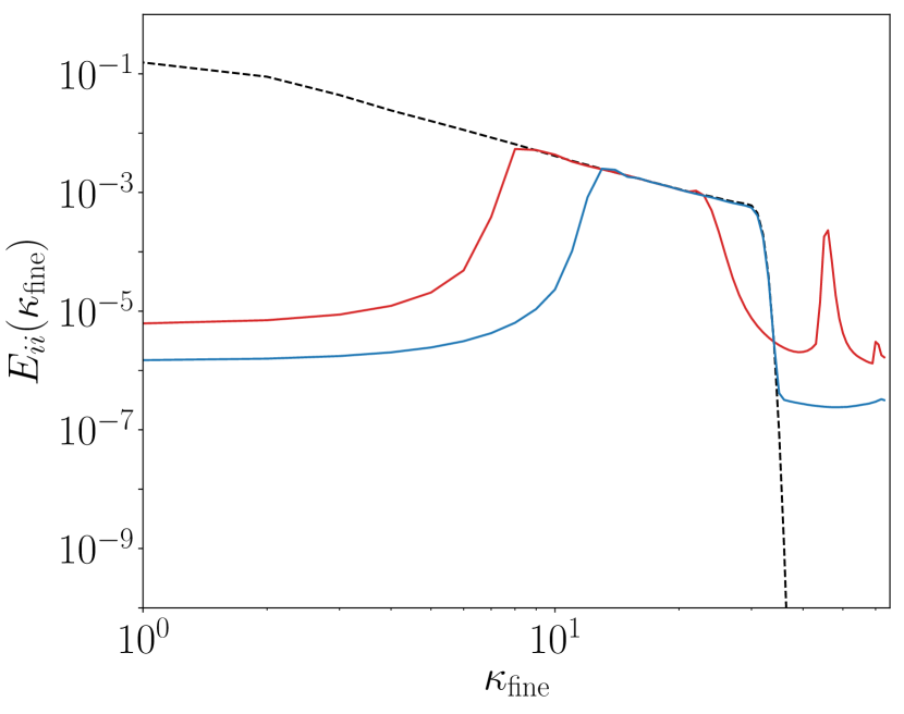
(b) $t=15.63({\color[rgb]{0.12109375,0.46484375,0.70703125}\rule[1.93748pt]{14.22636pt}{0.75pt}{}}),23.44$ ( )

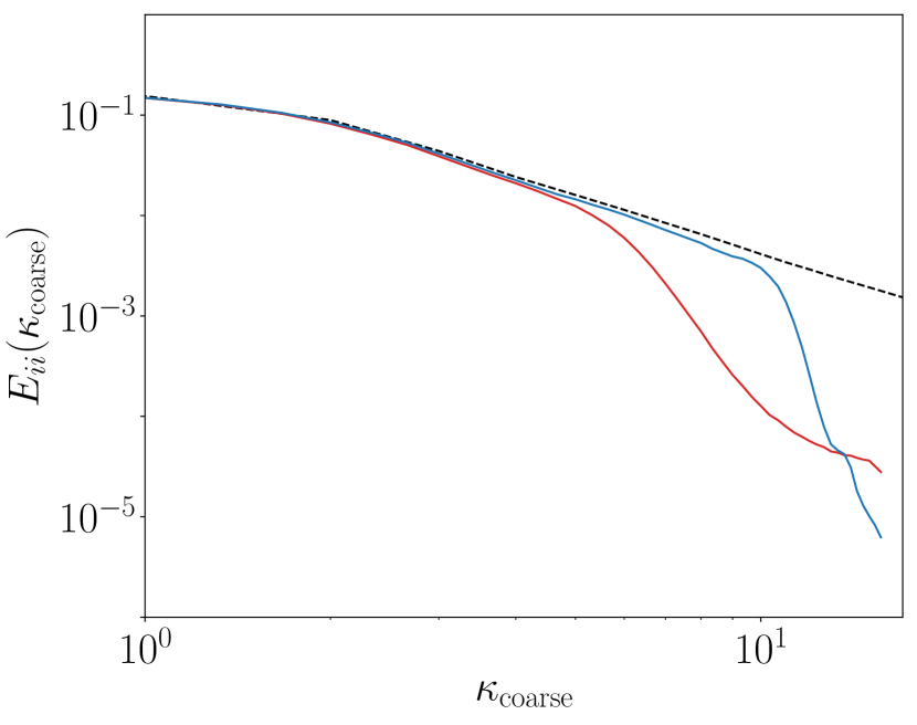
(c) $t=18.75({\color[rgb]{0.12109375,0.46484375,0.70703125}\rule[1.93748pt]{14.22636pt}{0.75pt}{}}),11.72$ ( )

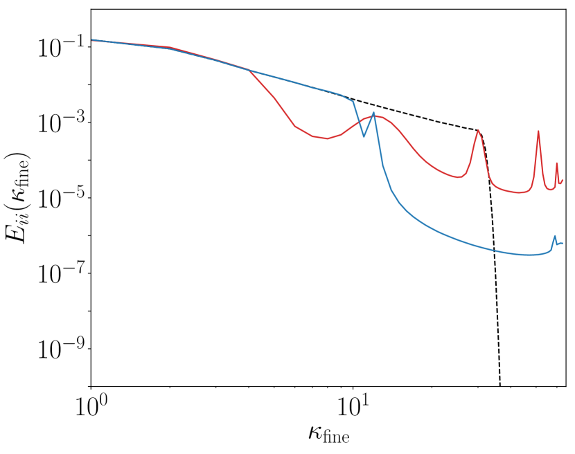
(d) $t=39.06({\color[rgb]{0.12109375,0.46484375,0.70703125}\rule[1.93748pt]{14.22636pt}{0.75pt}{}}),39.84$ ( )

Figure 4: One dimensional energy spectra, $E_{ii}$, in the direction of inhomogeneity at different times $t$; $\kappa_{\rm{fine}}$ and $\kappa_{\rm{coarse}}$ represent the wavenumbers in the fine and coarse regions of the domain, respectively. (a) High wavenumber reflections propagating backward through the fine region corresponding to the energy in the fine region in Fig. 3c. (b) The subsequent reflections propagating forward through the fine region corresponding to the energy in the fine region in Fig. 3d. (c) The spectra of the resolved turbulence packet in the coarse region corresponding to the energy in the coarse region in Fig. 3d. (d) The spectra of the turbulence packet after one flow through corresponding to the energy in the fine region in Fig. 3e.   (7th order B-splines),   (2nd order B-splines),       (Initial spectra of the turbulence packet shown in Fig. 3b).

The effects of resolution inhomogeneity on the spatial structure (see Fig. 3) and on the one dimensional energy spectra (see Fig. 4) of the turbulence packet are examined at several stages of the simulation for a single flow-through. Seventh-order B-splines and second-order B-splines are used to illustrate the behavior of higher- and lower-order methods. Based on the numerical analysis in Sec. II.2, the consistently normalized spectra of the $B_{1}^{2}$ and $B_{1}^{7}$ operators in the fine and coarse regions of the domain are sufficient to predict the behavior of the commutation error (see Fig 2(b)). To see this, let the wavenumbers $|\kappa|\in[0,16]$ be referred to as the coarse wavenumbers, wavenumbers $|\kappa|\in(16,32]$ be the fine wavenumbers, and wavenumber $|\kappa|\in(32,64]$ be the spurious wavenumbers, and recall that the fine region of the domain is capable of representing the fine, coarse, and spurious wavenumbers, while the coarse region is only capable of representing the coarse wavenumbers. The initial packet of turbulence only contains fine and coarse wavenumbers, so any energy transferred to higher wavenumbers by the resolution inhomogeneity is indeed spurious.

As the turbulence packet convects into the coarse region of the domain, all of the energy in the fine wavenumbers is transferred to scales with negative group velocity in the spurious wavenumber regime (see Fig 3c). As in Sec. II.2, this energy transfer occurs between wavenumbers that share an effective wavenumber. The corresponding energy spectra at this stage of the simulation show a pile up of energy in the largest wavenumbers in the fine region of the domain (see Fig 4(a)). Notice that, for each numerical scheme, the energy is concentrated in a narrow band of wavenumbers that corresponds to the region with negative slope in the effective wavenumbers shown in Fig. 2(b). The reflections in the second order B-spline case occur over a wider range of wavenumbers and are collectively more intense than for seventh-order case, as more energy is being reflected (see Fig 4(a)). Furthermore, the propagation speed of the reflections is much greater for seventh-order B-splines than second-order B-splines, as indicated by the slopes of the effective wavenumbers. Interestingly, we observed that, for a B-spline collocation method, the ratio of the group velocity to the convection velocity of the highest wavenumber reflections for each B-spline order matches the order of the B-spline (e.g., the Nyquist wavenumber propagates at negative $N$ times the convection velocity for $N$th order B-splines). This appears to be a special property of B-spline collocation that deserves proof and is consistent with the work of Vichnevetsky and Scheidegger [43], who demonstrated that an infinite speed of reflection occurs for spectral numerics.

Once the reflected fluctuations reach the resolution change on the left side of the fine region, they are reflected back into the fine region with positive group velocity with their initial wavenumbers. This re-reflection can be tracked from Fig. 3c in which the reflected wavepacket consisting of spurious wavenumbers is visible on the left-hand side as it propagates upstream (to the left), to Fig. 3d in which the re-reflected wavepacket consisting now of fine wavenumbers is visible propagating down-stream. These secondary reflections occur in the fine wavenumber regime but are as erroneous as the spurious reflections that created them. For both B-spline orders, the energy spectra in the fine resolution region for the initial turbulence packet and the reflected scales of motion match for all fine wavenumbers (see Fig. 4(b)). This indicates a total reflection occurs for all scales that are only representable on the fine grid, which agrees with the analysis of the $P_{2}$-type waves discussed in Sec. II.2. Without the commutator $\mathscr{C}^{I}$, this cycle of reflection between fine and spurious wavenumbers repeats. The energy initially contained in the fine wavenumber regime gets trapped in the fine resolution region.

The only fluctuation scales that make it through to the coarse region of the domain are those that can be represented on the coarse grid, i.e., the coarse wavenumbers (see Fig. 3d). The energy spectra at the initial time, and after the packet has convected into the coarse region, match almost identically for all coarse wavenumbers (see Fig. 4(c)). A relatively small fraction of the energy in the coarse wavenumbers also gets trapped in the fine region, as shown in Fig. 4(b). This behavior is also predicted by the numerical analysis of the $P_{1}$-type waves discussed in Sec. II.2, and would vanish in the limit of a smoothly varying grid.

The numerical experiment described here focuses on the idealized case of frozen turbulence consistent with Taylor’s hypothesis to emphasize the impact of commutation error. The scales trapped in the fine region of the domain are physically incorrect and numerically problematic. An increase in high wavenumber energy can lead to numerical instabilities, and the trapped low wavenumber energy can corrupt otherwise meaningful statistics. Moreover, it is reasonable to expect that in an LES nonlinear effects would magnify these problems as erroneous fluctuations would interact with and contaminate incoming turbulence. Consider, for instance, the turbulence packet after one flow through (see Fig. 3e). As the coarsely resolved packet re-enters the fine region (without any active forcing), the spectrum gets corrupted by the trapped energy (see Fig. 4(d)). Furthermore, a shift in energy from lower wavenumbers to higher wavenumbers would be particularly damaging in real turbulence as the former are more responsible for momentum transport while the latter are more responsible for dissipation. The nonlocal wavenumber interactions introduced by resolution inhomogeneity may corrupt the energy cascade, which, in homogeneous isotropic turbulence, is known to be dominated by interactions local in wavespace [44]. Lastly, notice that unlike the effects of discretization error, the effects of resolution inhomogeneity do not improve with higher-order numerics. Further study of these effects in an actual LES is warranted, but is out of scope for this paper. However, it is clear that a model for the inhomogeneous part of the commutator is needed to mitigate the effects of the commutation error.

IV Commutator Modeling

In this section we propose an approach to modeling the inhomogeneous commutator based on the characteristics of the commutator and the commutation error explored in Sec. II. As previously discussed, a model for the commutator is responsible for transferring energy between resolved and unresolved scales as a consequence of the resolution inhomogeneity. In the coarsening grid case, a commutation model must transfer the energy in newly unresolvable scales to the subgrid scales. In the refining grid case, a model for $\mathscr{C}^{I}$ would have to transfer energy from the subgrid to the resolved turbulence, presumably through some type of forcing. Notice that the requirements of a commutation model in the coarsening and refining cases are fundamentally different. It has been suggested that a “good” commutation model should handle both of these scenarios (e.g., [9]), however, because of these different requirements, this may not be appropriate. A commutation model for the coarsening and refining grid cases may need to be developed independently. We pursue this modeling approach here for the case of flow through coarsening grids to address the issues discussed in Sec. III.

A common mechanism for providing the transfer of energy from resolved to subgrid scales is a viscosity-based model, as suggested by the second order term in (6), which is equipped with the viscosity $\nu_{comm}=U\Delta\partial\Delta/\partial x$. However, as indicated by (8), a commutation model should ideally only affect wavenumbers near the cutoff wavenumber. This property preserves wavenumbers that are well resolved throughout the resolution change while removing those that are not. As such, a hyperviscosity is a more appropriate model for the commutator, as also indicated by the leading order terms in (6). Specifically, the leading order terms in (6) suggest the following form for a general one dimensional hyperviscosity commutation model:

$$\begin{split}U\mathscr{C}^{I}(u)\simeq(-1)^{N/2}CU\Delta\frac{d\Delta}{dx}\left(\Delta^{N-2}\frac{\partial^{N}\overline{u}}{\partial x^{N}}\right)\end{split},$$ (18)

for some constant $C$ and even order $N$ ($N$ is assumed to be a positive even integer for the remainder of this paper).

For any finite value of $N$ in (18), there is a trade-off between removing high wavenumber scales in fine regions of the grid that are approaching unresolvability, and preserving the well-resolved scales in coarse regions of the grid. Larger values of $N$ lead to sharper filters, which perform better in the context of this trade-off than smaller values of $N$. Accordingly, it is desirable to make $N$ as large as possible. Again, this is consistent with (8). However, the number of available derivatives of the filtered field limits how large $N$ can be, i.e., the underlying numerics constrain $N$ based on the number of accessible derivative operators. For example, CFD codes typically only have access to second derivative operators so that $N$ would be limited to $2$. Furthermore, larger values of $N$ require not only higher order numerics but also additional boundary conditions, which are often mentioned as a problem with hyperviscosity models [45, 3]. With this discussion in mind, we let (18) serve as the foundation for developing a one dimensional commutation model. The following subsections propose strategies for improving the model.

IV.1 The $B_{2}-B_{1}B_{1}$ Model

Let $F_{N}(u)\approx\partial^{N}u/\partial x^{N}$ be some numerical operator that approximates the $N$th derivative. The commutation model (18) can then be written as:

$$\mathscr{C}^{I}(u)=(-1)^{N/2}C\Delta\frac{d\Delta}{dx}\left(\Delta^{N-2}F_{N}(\overline{u})\right).$$ (19)

As mentioned above, it is desirable to take $N$ large, but the underlying numerics often limit $N$. However, lower-order numerical operators can be designed to mimic higher-order filters without increasing the order of the differential equation. For instance, consider the operator given by the difference between the numerical second derivative operator, $B_{2}$, and repeated application of the numerical first derivative operator, $B_{1}B_{1}$, (for a general numerical scheme). Figure 5 shows each of these operators for second-order centered difference numerics and several orders of B-splines. A simple Taylor expansion for second-order centered difference numerics gives:

$$\begin{split}(B_{2}^{CD}-B_{1}^{CD}B_{1}^{CD})u&\equiv\frac{-u_{j+2}+4u_{j+1}-8u_{j}+4u_{j-1}+u_{j-2}}{4\Delta^{2}}=-\frac{\Delta^{2}}{4}\frac{d^{4}u}{dx^{4}}+\mathcal{O}(\Delta^{4})\sim-\Delta^{2}F_{4}(u)\end{split}.$$ (20)

Similarly, it can be shown that $(B_{2}^{7}-B_{1}^{7}B_{1}^{7})u\sim\Delta^{8}\frac{d^{10}u}{dx^{10}}\approx\Delta^{8}F_{10}(u)$ and $(B_{2}^{2}-B_{1}^{2}B_{1}^{2})u\sim-\Delta^{2}\frac{d^{4}u}{dx^{4}}\approx-\Delta^{2}F_{4}(u)$. In all of these cases, $(-1)^{N/2+1}(B_{2}-B_{1}B_{1})\sim\Delta^{N-2}F_{N}$ for some value of $N$ (and positive constant of proportionality), which corresponds exactly to the form of (19); i.e.,

$${\mathscr{C}^{I}(u)=-C\Delta\frac{d\Delta}{dx}\left(B_{2}-B_{1}B_{1}\right)\bar{u}}.$$ (21)

The $B_{2}-B_{1}B_{1}$ operator has the effect of higher order differential operators without changing the order of the differential equation. This avoids the need to explicitly define higher order derivative approximations and for additional boundary conditions. Furthermore, the $B_{2}-B_{1}B_{1}$ operator is particularly useful because the first and second differential operators are already required by the governing equations, and are thus readily available in practical applications.

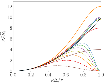
Figure 5: The spectrum of the second derivative operators ($\widehat{B_{2}}$) for a B-spline collocation method of several orders, a second-order centered difference method, and a spectral method. Repeated application of the first derivative operators are shown by the corresponding dashed lines;  ,      ($B_{2}^{2},B_{1}^{2}B_{1}^{2}$)  ,      ($B_{2}^{3},B_{1}^{3}B_{1}^{3}$)  ,      ($B_{2}^{4},B_{1}^{4}B_{1}^{4}$)  ,      ($B_{2}^{5},B_{1}^{5}B_{1}^{5}$)  ,      ($B_{2}^{6},B_{1}^{6}B_{1}^{6}$)  ,      ($B_{2}^{7},B_{1}^{7}B_{1}^{7}$)  ,      ($B_{2}^{CD},B_{1}^{CD}B_{1}^{CD}$)   (Spectral).

Aside from approximating higher order derivatives, the $B_{2}-B_{1}B_{1}$ operator has several desirable properties that make it useful for commutation modeling. Compare the second derivative operator, $B_{2}$, with repeated application of the first derivative operator, $B_{1}B_{1}$, in Fig. 5; for numerically well-resolved wavenumbers, the $B_{2}$ and $B_{1}B_{1}$ operators are almost identical, and they cancel out. However, for insufficiently resolved wavenumbers, their difference is nonzero and can be used to filter out higher wavenumbers. In essence, the $B_{2}-B_{1}B_{1}$ operator acts as an indicator for the scales whose dynamics are not sufficiently representable by the underlying numerics. This property is particularly useful for reducing commutation error as the $B_{2}-B_{1}B_{1}$ model is specifically formulated to damp wavenumbers with negative group velocity, which is where the commutation error manifests for many typical numerical schemes. Moreover, the operator naturally adapts to the underlying numerics.

IV.2 Model Coefficient

In an LES, the statistical analysis in Sec. II.1.2 can be used to set the model coefficient $C$ to produce the correct rate of energy transfer to the subgrid scales (e.g., evaluating (9) or (10) for a Kolmogorov spectrum). However, for the simple case of linear convection considered here, it is useful to examine how the behavior of the model changes as the coefficient varies. In Appendix C, a coefficient for this purpose is derived, which is repeated here,

$$C=\frac{(-1)^{\frac{N-2}{2}}\log(\varepsilon)}{2\left(\frac{\Delta_{c}-\Delta_{f}}{\Delta_{c}}\right)\left(\Delta^{N}\hat{F}_{N}(\kappa_{a})\right)},$$ (22)

where $\varepsilon$ is a tolerance level indicating the target fraction of incident energy that will be reflected, and ${\hat{F}}_{N}(\kappa)$ is the spectrum of $F_{N}$ evaluated at the wavenumber $\kappa$. Setting the parameter $\varepsilon$ involves a tradeoff between dissipating erroneous reflections in fine regions of the grid and preserving well-resolved wavenumbers in coarse regions of the grid.

Furthermore, this choice of coefficient may indicate how the numerical properties of the commutation error discussed in Sec. II.2 can be exploited to improve the model. To elaborate, notice that we use the value of $\hat{F}_{N}$ at the apex wavenumber $\kappa_{a}$. This choice is made to take advantage of how the commutation error manifests numerically. Specifically, the constant is designed to quickly damp high wavenumbers after they have been reflected. Targeting reflections yields a larger separation between the scales that must be filtered out, and those that need to be preserved. This approach is especially advantageous for low values of $N$ for which the filters produced from (18) are not particularly sharp. In essence, it is more advantageous to use a model to correct for the absence of $\mathscr{C}^{I}$ in this problem, than to model $\mathscr{C}^{I}$ directly. This strategy works particularly well with the $B_{2}-B_{1}B_{1}$ filters described in the previous section, which target the poorly resolved wavenumbers. In LES, more work is needed to see if a similar exploit can be performed. For example, nonlinear interactions may require scales to be removed before reflection, but this would lead to more dissipation of the resolved turbulence.

The spectrum of the operator $CF_{N}$ for second- and seventh-order B-splines with this choice of coefficient and several different choices of $N$ is shown is shown in Fig. 6. For an arbitrary tolerance value of $\varepsilon$, the model coefficient creates an intersection point at $\kappa_{a}$ between different values of $N$. This intersection point shifts depending on the order of the underlying numerics. Figure 6 shows how as $N$ increases, the poorly resolved scales are dissipated more rapidly and the well resolvable scales are better preserved.

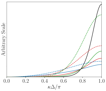
Figure 6: Spectra of the operator $CF_{N}$ for various forms of $F_{N}$ and the constant $C$ determined by (22). The scale is arbitrary and depends on $\varepsilon$ and the resolution $\Delta$.   ($F_{2}=B_{2}^{7}$),   ($F_{4}=B_{4}^{7}$),   ($F_{6}=B_{6}^{7}$),   ($\Delta^{8}F_{10}\sim B_{2}^{7}-B_{1}^{7}B_{1}^{7}$),       ($F_{2}=B_{2}^{2}$),       ($\Delta^{2}F_{4}\sim B_{2}^{2}-B_{1}^{2}B_{1}^{2}$),       ($F_{6}=(B_{2}^{2})^{3}$).

IV.3 Model Results

Figure 7: Convection of a packet of homogeneous, isotropic turbulence through an anisotropic, inhomogeneous grid with seventh-order B-splines, a convection velocity of 1, and a commutation model with $\Delta^{8}F_{10}\sim(B_{2}^{7}-B_{1}^{7}B_{1}^{7})$ and $\varepsilon=0.001$. The packet is moving through the resolution change to the right. (a) A slice of the numerical grid. (b), (c), (d), and (e) show the streamwise velocity field at times $0.00$, $7.03$, $11.72$, and $39.06$, respectively. Figure (c) is scaled to highlight the absence of the spurious high wavenumber reflections, as in Figure 3c.

The ability of the model to correct for the issues related to resolution inhomogeneity is tested in the same setting described in Sec. III. The commutation model is introduced into equation (16) as

$$\frac{\partial\overline{\mathbf{u^{\prime}}}}{\partial t}+U_{x}\frac{\delta\overline{\mathbf{u^{\prime}}}}{\delta x}=(-1)^{\frac{N}{2}+1}C\Delta_{x}\left(U_{x}\frac{\partial\Delta_{x}}{\partial x}\right)\left(\Delta_{x}^{N-2}F_{N}(\overline{\mathbf{u^{\prime}}})\right),$$ (23)

where the constant $C$ is given by (22), and the operator $F_{N}$ is an approximation of the $N$th derivative in the $x$-direction ($F_{N}\approx\partial^{N}/\partial_{x}^{N})$. Recall that in this setting the local grid spacing is $\boldsymbol{\Delta}(x)=(\Delta_{x}(x),\Delta_{y},\Delta_{z})$ and the dependence on $x$ in (23) arises because the resolution inhomogeneity is only in the $x$-direction.

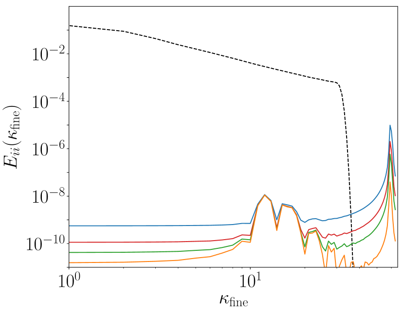
(a) $t=7.03$

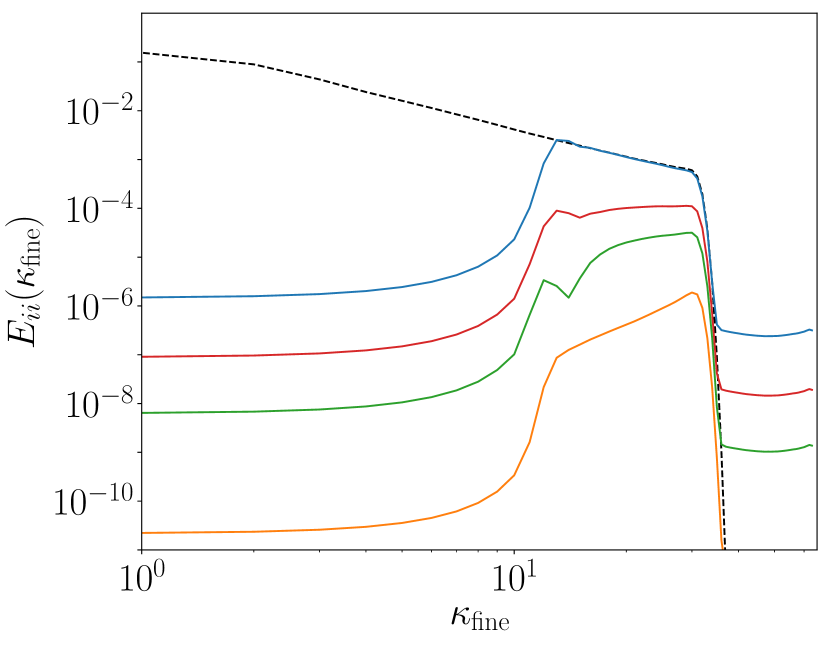
(b) $t=15.63$

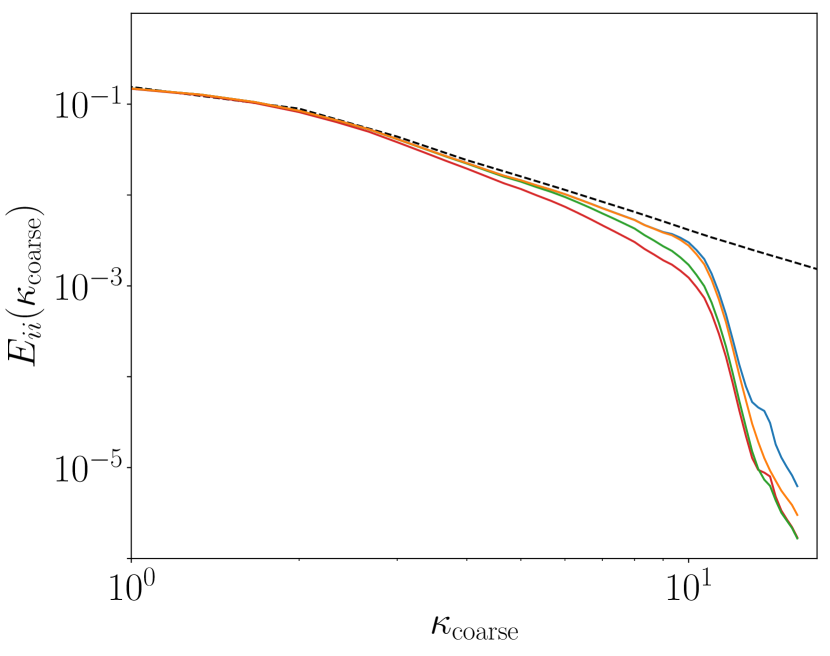
(c) $t=11.72$

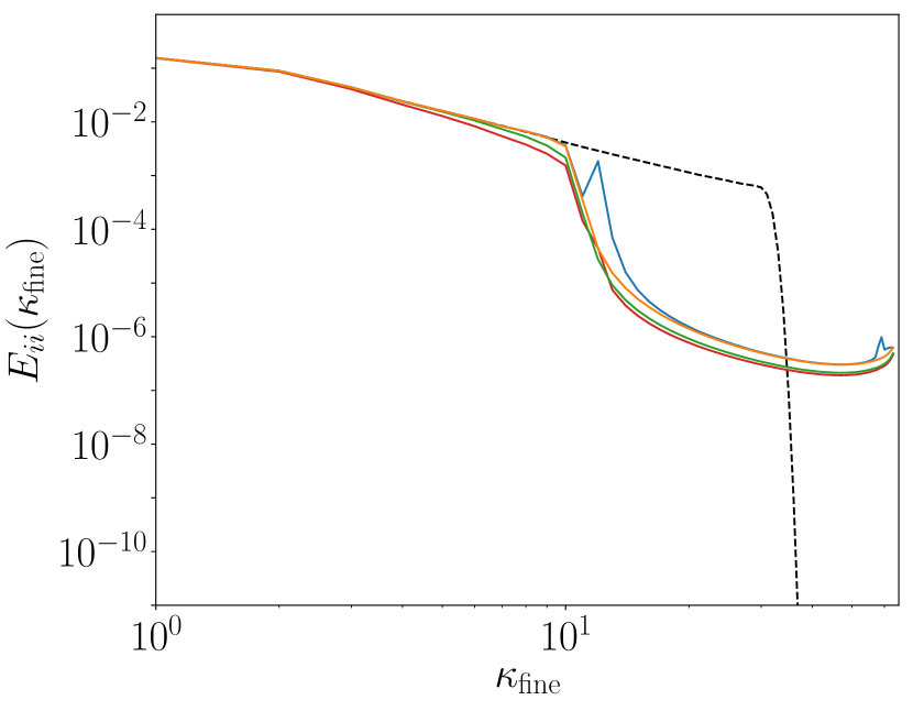
(d) $t=39.06$

Figure 8: Energy spectra, $E_{ii}$, in the direction of convection at different times $t$ for 7th order B-splines; $\kappa_{\rm{fine}}$ and $\kappa_{\rm{coarse}}$ represent the wavenumbers in the fine and coarse regions of the domain, respectively. (a) High wavenumber reflections propagating backward through the fine region. (b) The subsequent reflections propagating forward through the fine region. (c) The spectra of the resolved turbulence packet in the coarse region. (d) The spectra of the turbulence packet after one flow through.   (No model),   ($F_{2}=B_{2}^{7}$, $\varepsilon=0.1$),   ($F_{4}=B_{4}^{7}$, $\varepsilon=0.01$),   ($\Delta^{8}F_{10}\sim(B_{2}^{7}-B_{1}^{7}B_{1}^{7})$, $\varepsilon=0.001$),       (Initial Packet)

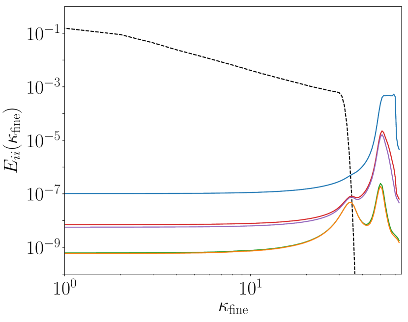
(a) $t=11.72$

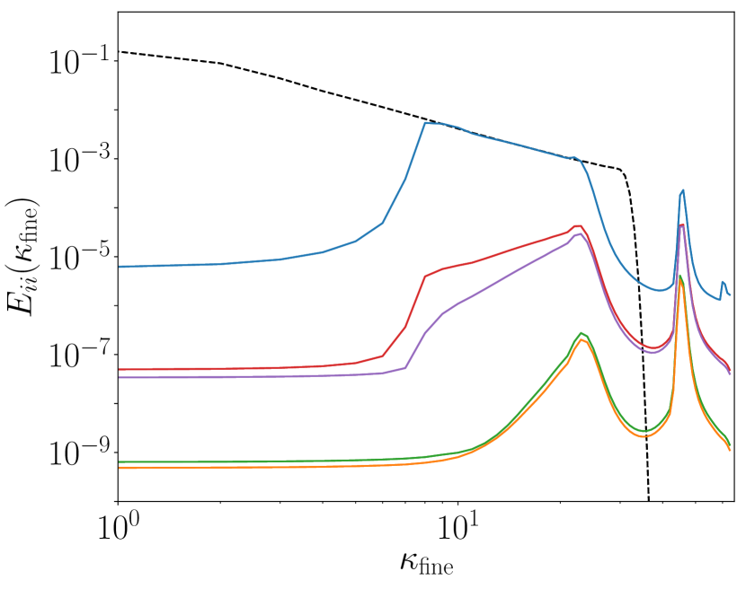
(b) $t=23.44$

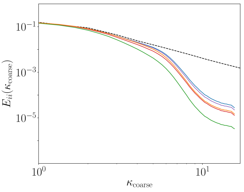
(c) $t=11.72$

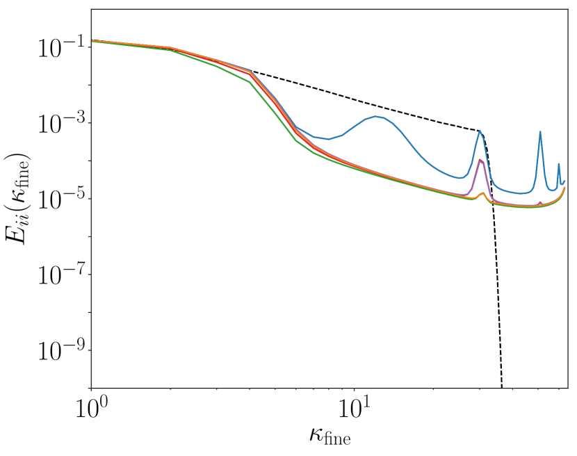
(d) $t=39.84$

Figure 9: Energy spectra, $E_{ii}$, in the direction of convection at different times $t$ for 2nd order B-splines; $\kappa_{\rm{fine}}$ and $\kappa_{\rm{coarse}}$ represent the wavenumbers in the fine and coarse regions of the domain, respectively. (a) High wavenumber reflections propagating backward through the fine region. (b) The subsequent reflections propagating forward through the fine region. (c) The spectra of the resolved turbulence packet in the coarse region. (d) The spectra of the turbulence packet after one flow through.   (No model),   ($\Delta^{2}F_{4}\sim-(B_{2}^{2}-B_{1}^{2}B_{1}^{2})$, $\varepsilon=0.1$),   ($\Delta^{2}F_{4}\sim-(B_{2}^{2}-B_{1}^{2}B_{1}^{2})$, $\varepsilon=0.001$),   ($F_{2}=B_{2}^{2}$, $\varepsilon=0.001$),   ($F_{2}=B_{2}^{2}$, $\varepsilon=0.1$),       (Initial Packet)

Table 1: Model Constants.

$N$	$F_{N}$	$\varepsilon$	$C$
$2$	$B_{2}^{7}$	$0.1$	$0.24$
$4$	$B_{4}^{7}$	$0.01$	$0.07$
$10$	$\Delta^{-8}(B_{2}^{7}-B_{1}^{7}B_{1}^{7})$	$0.001$	$4.31$
$2$	$B_{2}^{2}$	$0.1$	$0.38$
$2$	$B_{2}^{2}$	$0.001$	$1.15$
$4$	$-\Delta^{-2}(B_{2}^{2}-B_{1}^{2}B_{1}^{2})$	$0.1$	$0.76$
$4$	$-\Delta^{-2}(B_{2}^{2}-B_{1}^{2}B_{1}^{2})$	$0.001$	$2.28$

For the seventh-order B-spline results, three different choices of $N$ and $\varepsilon$ are tested: $N=2$ corresponding to the second derivative operator $F_{2}=B_{2}^{7}$ with $\varepsilon=0.1$, $N=4$ corresponding to the fourth derivative operator $F_{4}=B_{4}^{7}$ with $\varepsilon=0.01$, and $N=10$ corresponding to the $\Delta^{8}F_{10}\sim B_{2}^{7}-B_{1}^{7}B_{1}^{7}$ operator with $\varepsilon=0.001$. For the second-order B-spline results, two choices of $N$ are tested for both $\varepsilon=0.1$ and $\varepsilon=0.001$: $N=2$ corresponding to the $F_{2}=B_{2}^{2}$ operator, and $N=4$ corresponding to the $\Delta^{2}F_{4}\sim-(B_{2}^{2}-B_{1}^{2}B_{1}^{2})$ operator. These values, along with the model coefficients, are listed in Table 1. The one-dimensional energy spectra in the fine and coarse regions of the domain are shown in Fig. 8 and Fig. 9 for seventh- and second-order B-splines, respectively. The results of the model in physical space for the seventh order B-spline case with $\Delta^{8}F_{10}\sim(B_{2}^{7}-B_{1}^{7}B_{1}^{7})$ and $\varepsilon=0.001$ are shown in Fig. 7.

Compare these results with the pure convection case (i.e., the no model case) examined in Sec. III. The model significantly corrects the spatial structure and the energy distribution of the turbulence packet as it flows through the inhomogeneous grid. In all cases, the model reduces the spurious high wavenumber reflections by (at least) a factor around $\varepsilon$, as desired (see Figs 8(b) and 9(b)). Recall that the largest initial wavenumber with positive group velocity has the smallest reflected wavenumber and is dissipated the least by the model, so the value of $\varepsilon$ should be validated at these wavenumbers in the spectra results. Moreover, the model preserves the resolvable turbulence in the coarse region as much as possible. The seventh-order results show that higher order filters (i.e., larger values of $N$) preserve the resolvable turbulence while dissipating the reflections more strongly. In particular, the $B_{2}^{7}-B_{1}^{7}B_{1}^{7}$ model matches the ideal spectra in the coarse region almost exactly and is still able to reduce reflections by at least three orders of magnitude (see Fig 8(c)). Similarly, in the second-order B-spline results, the $N=4$ cases match the original spectra in the coarse region more closely than the $N=2$ cases for the same value of $\varepsilon$ (see Fig 9(c)). Finally, the model mitigates the effect of erroneous reflections on incoming turbulence, as demonstrated by examining the turbulence packet after one flow through (see Figs. 8(d) and 9(d)). Even a modest reduction in the reflections — such as that from the low $N$ and $\varepsilon$ cases — yields much better spectra than the pure convection case. The spectra after one flow through match quite well with the initial packet’s spectrum for all coarse wavenumbers.

V Conclusion

Practical LES of high Reynolds number turbulent flows often requires inhomogeneous resolution. The inhomogeneous part of the commutator $\mathscr{C}^{I}$ is responsible for transferring energy between resolved and unresolved scales as a consequence of the resolution inhomogeneity, and so it must be modeled. However, $\mathscr{C}^{I}$ is often ignored in practice leading to commutation error. In this paper, we investigate the commutator and corresponding commutation error as related to filters that include a discrete projection.

The impact of the commutation error that occurs as turbulence convects through coarsening grids is governed by the propagation properties of the underlying numerics (see Sec. II.2). For many conservative numerical schemes such as those considered here, the energy in newly unresolvable scales is unphysically transferred to higher wavenumbers in the fine region of the grid, instead of to the subgrid scales in the coarse region of the grid. The result is a non-physical reflection of unresolvable scales back into the fine region of the grid at higher wavenumbers with negative group velocities. The nonlocal wavenumber interactions introduced by resolution inhomogeneity may be especially problematic in LES of turbulence (see Sec. III). Since the implicit filter combined with the numerical derivative operators define the scales in the resolved field whose dynamics are accurately represented, LES modeling in general cannot be pursued independently of the properties of the numerics (e.g., [11, 23, 39, 46, 15]). As Meneveau and Katz [8] mentioned in their review paper, “our understanding of the interplay between numerical and modeling issues is presently quite limited.” The work here aims to address this interplay in the context of commutation error.

The statistical analysis of the commutation term $\mathscr{C}^{I}$ developed in Sec. II.1.2 yields a quantitative measure of the magnitude of $\mathscr{C}^{I}$ and therefore how important it is to model, as a function of the resolution gradient and the convection velocity. Furthermore, a commutator model can be formulated to match important statistical features of the commutator a priori, such as its spectrum. For example, the dependence of the commutator spectrum on the derivative of the Fourier transformed filter kernel shows that a commutator model should act at the high wavenumbers over which the filter rolls off. Similarly, the parameters in a model of the commutator can be calibrated to match known statistical characteristics a priori (e.g., evaluating (9) for a Kolmogorov spectrum). It is important to consider the statistical characteristics of the commutation term because a priori consistency of certain statistical characteristics of an LES model is a necessary condition for accurate a posteriori statistics of an LES solution [27, 24].

The series approximation of $\mathscr{C}^{I}$ from Sec. II.1.1, is also useful for informing commutation models, despite the fact that this analysis is formally only applicable to invertible filters. In particular, (7) shows that asymptotically, the commutator is expressible in terms of even derivatives of the filtered field, is proportional to the resolution gradient and proportional to the convection velocity. This places significant constraints on any operator intended to model the commutator. Furthermore, when applied to inertial range turbulence, the fact that all the terms in the series (7) are of the same asymptotic order implies that high order derivatives of the filtered field are as important as low order derivatives, suggesting that practical models expressed in terms of derivatives of the filtered field should include derivatives of as high an order as feasible. Indeed, this observation motivated the formulation of the model proposed in Sec. IV. The asymptotic ordering of the terms in (7) also suggests that using “commuting filters” whose low-order moments vanish, which has often been proposed based on the analysis of [1], is not sufficient to make the commutator negligible. This is not to say that explicit filters are not useful for other purposes, such as eliminating energy in scales with negative group velocity due to numerical dispersion, which will also mitigate the effects of commutation error.

For the case of flow through a coarsening grid, a practical formulation of a high-order dissipative model is proposed in Sec. IV. The model is based on the analysis in Sec. II and is formulated to be proportional to $B_{2}-B_{1}B_{1}$ ($B_{2}$ and $B_{1}$ are numerical second and first derivative operators), which avoids several practical complications with hyperviscosity models. In setting the model constant, there is a trade-off between eliminating the spurious reflections in the fine region and preserving the dynamically meaningful scales in the coarse region (see Sec. IV.2). Furthermore, the $B_{2}-B_{1}B_{1}$ operator could also be useful for addressing discretization error, which can dominate over the LES models and must therefore be considered in LES [15, 16, 17]. The $B_{2}-B_{1}B_{1}$ operator dissipates scales whose dynamics are poorly represented in an LES and adapts naturally to the underlying numerics without needing to define ad hoc filter widths or explicit filters. This aligns with previous work suggesting the use of hyperviscosities for mitigating the effects of discretization error [45].

Finally, the commutator modeling pursued here has focused on the case when the turbulence flows from fine resolution to coarse resolution. However, the other situation (flowing from coarse to fine resolution) is also of interest. Modeling $\mathscr{C}^{I}$ in this case is challenging because resolved fluctuations must be created. Models based on negative dissipation [1] and forcing [47], have been proposed, but more work is required. As in the coarsening resolution case, the analysis in Sec. II.1.1 and II.1.2 may be useful in developing an appropriate model.

Appendix A Multiscale Analysis of the Commutator

In this Appendix, we consider a multiscale asymptotic analysis of the inhomogeneous part of the commutator. This analysis is used to obtain the leading order terms in a series representation of the commutator in the case of invertible filters (Appendix A.1) and the statistical characteristics of the commutator for a general filter (Appendix A.2).

A.1 Series Representation of the Commutator

As in [1], any smoothly nonuniform grid $x$ with spacing $\Delta(x)$ can be mapped to a uniform grid of spacing $\Delta_{\xi}$ through some invertible monotonic differentiable mapping function $\xi=f(x)$. Let $G(\xi)$ be a symmetric filter kernel normalized on $\xi$ that decays sufficiently fast so that all moments of $G$ exist. To define the filtering operation applied to an arbitrary function $\psi(x)$, we first make a change of variables to $\xi$ ($\psi(\xi)\equiv\psi(f^{-1}(\xi))$) and then filter $\psi(\xi)$ with the homogeneous filter defined by $G(\xi)$:

$$\overline{\psi}(\xi)=\frac{1}{\Delta_{\xi}}\int G\left(\frac{\xi-\eta}{\Delta_{\xi}}\right)\psi(\eta)d\eta.$$ (24)

The result is then transformed back to $x$ to obtain:

$$\overline{\psi}(x)\equiv\overline{\psi}(f(x))=\frac{1}{\Delta_{\xi}}\int G\left(\frac{f(x)-f(y)}{\Delta_{\xi}}\right)\psi(y)f^{\prime}(y)dy.$$ (25)

Therefore $\displaystyle{\frac{d\overline{\psi}}{dx}\equiv\frac{d\overline{\psi}}{d\xi}\frac{d\xi}{dx}}$, so that the inhomogeneous part of the commutator is

$$\mathscr{C}^{I}(\psi)=\overline{\frac{d\psi}{dx}}-{\frac{d{\overline{\psi}}}{d\xi}}\frac{d\xi}{dx}$$ (26)

as in [24].

Now, suppose that the resolution (filter width) is slowly varying in $x$, that is $\frac{d\Delta}{dx}$ is order $\epsilon\ll 1$. Notice that this limit can be approached in two ways. In particular, consider the length scale $L_{\Delta}$ defined as the inverse logarithmic derivative of the resolution ($\frac{1}{L_{\Delta}}\sim\frac{1}{\Delta}\frac{d\Delta}{dx}$). Then the $\epsilon$ limit can be approached by (1) allowing $L_{\Delta}$ to grow while $\Delta$ remains constant, or (2) letting $L_{\Delta}$ remain constant while $\Delta$ goes to zero. In either case, (25) is asymptotically equivalent to

$$\overline{\psi}(x)=\frac{f^{\prime}(x)}{\Delta_{\xi}}\int G\left(\frac{f^{\prime}(x)(x-y)}{\Delta_{\xi}}\right)\psi(y)dy+\mathcal{O}({\epsilon}).$$ (27)

Further, in the case of an inhomogeneous filter with slowly varying resolution, a filtered quantity will vary over a long and short length scale, the scale of filter variation and the scale of resolved turbulent fluctuations, respectively. As such, we use (27) to facilitate a multiscale asymptotic analysis of the commutator in terms of a slow variable $w=\epsilon x$ and fast variable $\tilde{x}$. In this case, $\Delta$ depends on $w$, but not $\tilde{x}$. Since $f^{\prime}(x)=\Delta_{\xi}/\Delta(x)$, we have

$$\overline{\psi}(w,\tilde{x})=\frac{1}{\Delta(w)}\int G\left(\frac{\tilde{x}-y}{\Delta(w)}\right)\psi(y)dy.$$ (28)

In what follows, the dependence of $\Delta$ on $w$ is implied though no longer explicitly indicated. Using multiscale asymptotics, the derivative of $\overline{\psi}$ with respect to $x$ is written

$$\frac{d\overline{\psi}}{dx}=\frac{\partial\overline{\psi}}{\partial\tilde{x}}+\epsilon\frac{\partial\overline{\psi}}{\partial w}+\mathcal{O}(\epsilon^{2}).$$ (29)

Since the filter is homogeneous in $\tilde{x}$, $\displaystyle{\frac{\partial\overline{\psi}}{\partial\tilde{x}}=\overline{\frac{d\psi}{dx}}}$. Therefore, to leading order the commutator is given by

$$\mathscr{C}^{I}(\psi)=\overline{\frac{d\psi}{dx}}-\frac{d\overline{\psi}}{\partial x}=-\epsilon\frac{\partial\overline{\psi}}{\partial w},$$ (30)

which can be computed as

$$\mathscr{C}^{I}(\psi)=\frac{1}{\Delta^{2}}\frac{d\Delta}{dx}\int\left(\frac{\tilde{x}-y}{\Delta}G^{\prime}\left(\frac{\tilde{x}-y}{\Delta}\right)+G\left(\frac{\tilde{x}-y}{\Delta}\right)\right)\psi(y)\,dy.$$ (31)

where $G^{\prime}$ is the derivative of $G$ with respect to its argument. Introducing the variable $\zeta=(y-\tilde{x})/\Delta$ and expanding $\psi(y)$ in a Taylor series about $\tilde{x}$ gives

$$\begin{split}\mathscr{C}^{I}(\psi)&=\frac{1}{\Delta}\frac{d\Delta}{dx}\int\left(\zeta G^{\prime}\left(\zeta\right)+G\left(\zeta\right)\right)\left(\sum_{n=0}^{\infty}\frac{(\zeta\Delta)^{n}}{n!}\frac{d^{n}\psi}{dx^{n}}(\tilde{x})\right)d\zeta\\ &=\sum_{n=1}^{\infty}\left(\frac{-\Delta^{2n-1}}{(2n-1)!}\frac{d\Delta}{dx}\frac{d^{2n}\psi}{dx^{2n}}(\tilde{x})\int\zeta^{2n}G(\zeta)d\zeta\right)\end{split},$$ (32)

where we have used the fact that odd order moments of $G$ are zero. To express the commutator in terms of the filtered field $\overline{\psi}$, we first invert (28) using the same procedure to obtain

$$\begin{split}\psi(\tilde{x})=\overline{\psi}(w,\tilde{x})-\sum_{n=1}^{\infty}\frac{\Delta^{2n}}{(2n)!}\frac{d^{2n}\psi}{dx^{2n}}(\tilde{x})\int\zeta^{2n}G(\zeta)d\zeta.\end{split}$$ (33)

Then we can recursively substitute (33) into (32) to obtain an expression for the commutator in terms of $\overline{\psi}$. However, to properly order this expansion, the way in which derivatives of $\overline{\psi}$ and $\Delta$ scale with $\epsilon$ must be considered. When $\epsilon\rightarrow 0$ at constant $\Delta$, both $\overline{\psi}$ and $\Delta$ are order one in $\epsilon$. However, when $\epsilon\rightarrow 0$ at constant $L_{\Delta}$, $\Delta\sim\epsilon$ and, in general, the derivatives of $\overline{\psi}$ scale with powers of $\epsilon$. In high Reynolds number turbulence that has been filtered at scale $\Delta$ in the inertial range, the Kolmogorov scale similarity hypotheses for the statistics of velocity differences imply that the statistics of the derivatives of the filtered velocity $\overline{u}$ depend only on $\Delta$ and the rate of kinetic energy dissipation $\varepsilon_{k}$. Dimensional analysis then requires that the standard deviation of $\partial^{n}\overline{u}/\partial x^{n}$ scales as $\varepsilon_{k}^{2/3}\Delta^{1/3-n}$. Thus, taking $\psi$ to be $u$, the $n^{th}$ derivative of $\overline{u}$ in the series expansion will scale as $\epsilon^{1/3-n}$. Regardless of how the limit of small $\epsilon$ is approached, one obtains

$$\begin{split}\mathscr{C}^{I}(u)&=-M_{2}\Delta\frac{d\Delta}{dx}\frac{\partial^{2}\overline{u}}{\partial\tilde{x}^{2}}+\left(\frac{M_{2}^{2}}{2}-\frac{M_{4}}{6}\right)\Delta^{3}\frac{d\Delta}{dx}\frac{\partial^{4}\overline{u}}{\partial\tilde{x}^{4}}+\dots+C_{N}\Delta^{N-1}\frac{d\Delta}{dx}\frac{\partial^{N}\overline{u}}{\partial\tilde{x}^{N}}+\dots+\mathcal{O}(\epsilon^{q})\\ &=\sum_{n=1}^{\infty}\left(C_{2n}\Delta^{2n-1}\frac{d\Delta}{dx}\frac{\partial^{2n}\overline{u}}{\partial\tilde{x}^{2n}}\right)+\mathcal{O}(\epsilon^{q})\end{split},$$ (34)

where $q=2$ when the asymptotic limit is taken with constant $\Delta$ (the leading order series being order $\epsilon$) and $q=4/3$ when it is taken at constant $L_{\Delta}$ (the leading order series being order $\epsilon^{1/3}$). Here we let $M_{k}$ denote the $k$th order moment of the filter kernel, $N$ is even, and in general, the coefficient $C_{j}$ on the $j^{th}$ order term depends on the moments of the filter up to order $j$.

A.2 Spectral Characteristics of the Commutator

We turn our attention now to the spectral characteristics of the commutator. However, to make a connection to the statistical properties of the commutator in LES of turbulence, we consider instead a three-dimensional isotropic inhomogeneous filter, defined similarly to (27) as

$$\overline{\psi}(\mathbf{x})=\frac{1}{\Delta(\mathbf{x})^{3}}\int G\left(\frac{|\mathbf{x}-\mathbf{y}|}{\Delta(\mathbf{x})}\right)\psi(\mathbf{y})d\mathbf{y},$$ (35)

where $G$ is now a scalar function on $[0,\infty)$ satisfying $4\pi\int_{0}^{\infty}G(r)r^{2}\,dr=1$. The same multiscale expansion holds as above for the case where $\frac{\partial\Delta}{\partial x_{i}}\sim\mathcal{O}(\epsilon)$. The filtering operation can be expressed as

$$\overline{\psi}(\mathbf{w},\tilde{\mathbf{x}})=\frac{1}{\Delta(\mathbf{w})^{3}}\int G\left(\frac{|\tilde{\mathbf{x}}-\mathbf{y}|}{\Delta(\mathbf{w})}\right)\psi(\mathbf{y})d\mathbf{y},$$ (36)

where $\mathbf{w}=\epsilon\mathbf{x}$ is the slow variable and $\tilde{\mathbf{x}}$ is the fast variable, and the commutator, $\displaystyle{\mathscr{C}_{i}^{I}(\psi)=\overline{\frac{\partial\psi}{\partial x_{i}}}-\frac{\partial\overline{\psi}}{\partial x_{i}}=-\epsilon\frac{\partial\overline{\psi}}{\partial w_{i}}}$, can be computed as

$$\begin{split}\mathscr{C}_{i}^{I}(\psi)&=\frac{\epsilon}{\Delta^{4}}\frac{\partial\Delta}{\partial w_{i}}\int\left(\frac{|\tilde{\mathbf{x}}-\mathbf{y}|}{\Delta}G^{\prime}\left(\frac{|\tilde{\mathbf{x}}-\mathbf{y}|}{\Delta}\right)+3G\left(\frac{|\tilde{\mathbf{x}}-\mathbf{y}|}{\Delta}\right)\right)\psi(\mathbf{y})\,d\mathbf{y}\\ &\equiv\int\mathcal{C}_{i}(\mathbf{w},\tilde{\mathbf{x}}-\mathbf{y})\psi(\mathbf{y})d\mathbf{y}\end{split},$$ (37)

Furthermore, because the filter is homogeneous in the fast variable, it is useful to consider the Fourier transform of $\overline{\psi}$ in the fast variable:

$$\widehat{\overline{\psi}}(\mathbf{w},\boldsymbol{\kappa})=\frac{1}{(2\pi)^{3}}\int\overline{\psi}(\mathbf{w},\tilde{\mathbf{x}})e^{-i\boldsymbol{\kappa}\cdot\tilde{\mathbf{x}}}\,d\tilde{\mathbf{x}}.$$ (38)

Applying the convolution theorem to (36) yields $\displaystyle{\widehat{\overline{\psi}}(\mathbf{w},\boldsymbol{\kappa})=\widehat{\psi}(\boldsymbol{\kappa})\widehat{G}(\Delta|\boldsymbol{\kappa}|)}$, where $\widehat{\psi}$ is the Fourier transform of $\psi$ and $\widehat{G}(|\boldsymbol{\kappa}|)=\frac{1}{(2\pi)^{3}}\int G(|\mathbf{z}|)e^{-i\boldsymbol{\kappa}\cdot\mathbf{z}}\,d\mathbf{z}$ is the Fourier transform of the filter kernel, which depends only on $|\boldsymbol{\kappa}|$ because $G(|\mathbf{z}|)$ is isotropic. Note that because the unfiltered quantity $\psi$ does not depend on $\Delta$, it also does not depend on $\mathbf{w}$. The Fourier transform of the commutator is thus given by

$$\widehat{\mathscr{C}_{i}^{I}}(\psi)=-\epsilon\frac{\partial\widehat{\overline{\psi}}}{\partial w_{i}}(\mathbf{w},\boldsymbol{\kappa})=-\widehat{\psi}(\boldsymbol{\kappa})\frac{\partial\widehat{G}(\Delta|\boldsymbol{\kappa}|)}{\partial x_{i}}=-\widehat{\psi}(\boldsymbol{\kappa})\widehat{G}^{\prime}(\Delta|\boldsymbol{\kappa}|)|\boldsymbol{\kappa}|\frac{\partial\Delta}{\partial x_{i}}\equiv-\widehat{\mathcal{C}}_{i}(\mathbf{w},\boldsymbol{\kappa})\widehat{\psi}(\boldsymbol{\kappa}).$$ (39)

where $\widehat{G}^{\prime}$ is the derivative of $\widehat{G}$ with respect to its argument.

While (37) and (39) provide explicit expressions for the commutator, they require knowledge of the unfiltered field $\psi$ or its Fourier transform. If $G$ were invertible, we could relate $\psi$ and $\overline{\psi}$ as in (33), but this is not the case for non-invertible filters, such as those that include a finite dimensional projection. As such, this information is generally not available in an LES, however, we may have theory or models for the statistics of $\psi$, which could allow us to determine the statistics of the commutator.

Consider, for example, homogeneous, isotropic turbulence flowing through an inhomogeneous grid at a velocity $U_{i}$ that is much greater than the fluctuations $u_{i}$ so that Taylor’s frozen field hypothesis holds, as in Sec. III. In this case, Kolmogorov theory provides a model for the spectrum tensor $\phi_{ij}(\boldsymbol{\kappa})=\int\langle\widehat{u}_{i}(\boldsymbol{\kappa}^{\prime})\widehat{u}^{*}_{j}(\boldsymbol{\kappa})\rangle\,d\boldsymbol{\kappa}^{\prime}$, $*$ denotes complex conjugate, $\widehat{u}_{i}$ is the Fourier transform of the velocity, and $\phi_{ij}$ is also the Fourier transform of the two-point correlation tensor. The spectrum tensor of the filtered velocity is given by $\overline{\phi}_{ij}(\boldsymbol{\kappa})=\widehat{G}^{2}(\Delta|\boldsymbol{\kappa}|)\phi_{ij}(\boldsymbol{\kappa})$. The commutator arising from the convection term in the filtered evolution equation is $U_{k}\mathscr{C}_{k}(u_{j})$, and its contribution to the evolution of $\overline{\phi}_{ij}$ is given by

$$\tilde{\mathscr{C}}^{I}(\overline{\phi}_{ij})=U_{k}\int\langle\widehat{\overline{u}}_{i}(\boldsymbol{\kappa}^{\prime})\widehat{\mathscr{C}_{k}^{I}}(u_{j})^{*}\rangle\,d\boldsymbol{\kappa}^{\prime}+U_{k}\int\langle\widehat{\overline{u}}^{*}_{j}(\boldsymbol{\kappa})\widehat{\mathscr{C}_{k}^{I}}(u_{i})\rangle\,d\boldsymbol{\kappa}^{\prime}=-2U_{k}\frac{\partial\Delta}{\partial x_{k}}\widehat{G}(\Delta|\boldsymbol{\kappa}|)\widehat{G}^{\prime}(\Delta|\boldsymbol{\kappa}|)|\boldsymbol{\kappa}|\phi_{ij}(\boldsymbol{\kappa})$$ (40)

where the $\tilde{\mathscr{C}}$ nomenclature indicates the contribution of the commutator to the evolution equation for its argument. The contribution of the commutator to the evolution of the filtered three-dimensional energy spectrum $\overline{E}(|\boldsymbol{\kappa}|)=2\pi|\boldsymbol{\kappa}|^{2}\overline{\phi}_{ii}(\boldsymbol{\kappa})$ and resolved turbulent kinetic energy $k^{>}=\int_{0}^{\infty}\overline{E}(\kappa)\,d\kappa$ can easily be obtained from (40) as:

$$\tilde{\mathscr{C}}^{I}(\overline{E}) =-2U_{k}\frac{\partial\Delta}{\partial x_{k}}\widehat{G}(\Delta\kappa)\widehat{G}^{\prime}(\Delta\kappa)\kappa E(\kappa)$$ (41)

$$\tilde{\mathscr{C}}^{I}(k^{>}) =-2U_{k}\frac{\partial\Delta}{\partial x_{k}}\int_{0}^{\infty}\widehat{G}(\Delta\kappa)\widehat{G}^{\prime}(\Delta\kappa)\kappa E(\kappa)\,d\kappa$$ (42)

Note that unlike the analysis in Appendix A.1, the analysis outlined here does not rely on deconvolution, and so is applicable to noninvertible filters that include implicit truncation. For example, if $G$ is a Fourier cutoff and $G^{\prime}$ is interpreted in the sense of distributions, then (42) simplifies to

$$\tilde{\mathscr{C}}^{I}(k^{>})=U_{k}\frac{\partial\kappa_{c}}{\partial x_{k}}E(\kappa_{c}),$$ (43)

where $\kappa_{c}$ is the cutoff wavenumber. Note that this multiscale analysis can also be generalized to the case of spatially varying anisotropic resolution.

Appendix B Generalizing the Analysis of Ghosal and Moin [1]

Ghosal and Moin [1] did not employ a multiscale asymptotic analysis such as that in Appendix A, however, their analysis can be interpreted asymptotically. In this appendix, we explore the relationship between the series analysis of Appendix A.1 and that of Ghosal and Moin, and extend the latter to characterize the asymptotically higher order terms.

Recall, the filtering of an arbitrary function $\psi(x)$ was defined in (25) as

$$\overline{\psi}(x)=\frac{1}{\Delta_{\xi}}\int G\left(\frac{f(x)-f(y)}{\Delta_{\xi}}\right)\psi(y)f^{\prime}(y)dy.$$ (44)

As in Ghosal and Moin [1], we work directly with (44) and obtain

$$\begin{split}\mathscr{C}^{I}(\psi)&=\int G(\zeta)\psi^{\prime}(y)\left[1-\frac{f^{\prime}(x)}{f^{\prime}(y)}\right]d\zeta\end{split}$$ (45)

for the inhomogeneous part of the commutator, where we have introduced the variable $\zeta=(f(y)-f(x))/\Delta_{\xi}$.

To expand (45) in a series of explicit powers of $\Delta_{\xi}$, we follow [1] but consider the general case including terms up to $\Delta_{\xi}^{N}$ for some $N$. By inverting the definition of $\zeta$, we can express $y$ as

$$y=\sum_{i=0}^{\infty}\Delta_{\xi}^{i}\zeta^{i}y_{i},$$ (46)

where $y_{0}=x$, $y_{1}=1/f^{\prime}(x)$ and $y_{i}$ is given by

$$y_{i}=-\sum_{n=2}^{i}\frac{\beta_{n,{i-n}}}{n!f^{\prime}(x)}\frac{d^{n}f}{dx^{n}},$$ (47)

where

$$\beta_{n,0}=y_{1}^{n},\qquad\beta_{n,m}=\frac{1}{my_{1}}\sum_{k=1}^{m}(kn-m+k)y_{k+1}\beta_{n,m-k}.$$ (48)

Then $(y-x)$ can be expressed as

$$(y-x)^{n}=\left(\sum_{m=1}^{\infty}\Delta_{\xi}^{m}\zeta^{m}y_{m}\right)^{n}=\sum_{j=0}^{N-n}\Delta_{\xi}^{j+n}\zeta^{j+n}\beta_{n,j}+\dots\;,$$ (49)

for $n>0$, which includes all terms with explicit powers of $\Delta_{\xi}$ up to some power $N$. Substitution of (49) into a general Taylor series expansion of $\psi(y)$ about $x$ gives:

$$\psi(y)=\psi(x)+\sum_{n=1}^{N}\left(\frac{\psi^{(n)}(x)}{n!}\sum_{j=0}^{N-n}\Delta_{\xi}^{j+n}\zeta^{j+n}\beta_{n,j}\right)+\dots\;.$$ (50)

Equation (50) can be used to expand each term in (45) about $x$ so that all the terms of the commutator with explicit powers of $\Delta_{\xi}$ up to some order $N$ is given by:

$$\begin{split}\mathscr{C}^{I}(\psi)&=\sum_{m=1}^{N}\left[\vphantom{\sum_{j=0}^{N-n}}\right.\frac{1}{m!}\left[\psi^{\prime}\left(\frac{1}{f^{\prime}}\right)^{(m)}f^{\prime}\right](x)\underset{k+m\in 2\mathbb{Z}}{\sum_{k=0}^{N-m}}\Delta_{\xi}^{k+m}\beta_{m,k}\int\zeta^{k+m}G(\zeta)d\zeta\left.\vphantom{\sum_{j=0}^{N-n}}\right]\\ &+\sum_{n=1}^{N}\sum_{m=1}^{N}\left[\vphantom{\sum_{j=0}^{N-n}}\right.\frac{1}{n!m!}\left[\psi^{(n+1)}\left(\frac{1}{f^{\prime}}\right)^{(m)}f^{\prime}\right](x)\underset{j+k+n+m\in 2\mathbb{Z}}{\underset{j+k+n+m\leq N}{\sum_{j=0}^{N-n}\sum_{k=0}^{N-m}}}\Delta_{\xi}^{j+k+n+m}\beta_{n,j}\beta_{m,k}\int\zeta^{j+k+n+m}G(\zeta)d\zeta\left.\vphantom{\sum_{j=0}^{N-n}}\right]\end{split}.$$ (51)

For example, for $N=2$ we obtain,

$$\mathscr{C}^{I}(\psi)=\left(\frac{f^{\prime\prime}}{f^{\prime 3}}\frac{d^{2}\psi}{dx^{2}}+\left(\frac{f^{\prime\prime\prime}}{2f^{\prime 3}}-\frac{3f^{\prime\prime 2}}{2f^{\prime 4}}\right)\frac{d\psi}{dx}\right)\Delta_{\xi}^{2}\int\zeta^{2}G(\zeta)d\zeta\;,$$ (52)

which agrees with equation (3.9) in [1].

To express the commutator in terms of $\overline{\psi}$, we follow the same procedure as (33). Inverting (44) gives

$$\psi(x)=\overline{\psi}(x)-\sum_{n=1}^{N}\left(\frac{\psi^{(n)}(x)}{n!}\underset{j+n\in 2\mathbb{Z}}{\sum_{j=0}^{N-n}}\Delta_{\xi}^{j+n}\beta_{n,j}\int\zeta^{j+n}G(\zeta)d\zeta\right)+\dots\;.$$ (53)

Equation (53) can be recursively substituted into (51) to obtain the commutator in terms of the filtered velocity field. Moreover, the commutator can be expressed in terms of the local grid spacing $\Delta(x)$ using the relationship $f^{\prime}=\Delta_{\xi}/\Delta$. The terms with explicit powers of $\Delta_{\xi}$ up to $N=2$ are

$$\mathscr{C}^{I}(\psi)=\left(-\left[\frac{1}{2}\left(\Delta^{\prime 2}+\Delta\Delta^{\prime\prime}\right)\right]\frac{d\overline{\psi}}{dx}-\left[\Delta\Delta^{\prime}\right]\frac{d^{2}\overline{\psi}}{dx^{2}}\right)\int\zeta^{2}G(\zeta)d\zeta.$$ (54)

For $N=4$ we obtain,

$$\begin{split}\mathscr{C}^{I}(\psi)&=-\left[\frac{1}{2}\left(\Delta^{\prime 2}+\Delta\Delta^{\prime\prime}\right)\right]\frac{d\overline{\psi}}{dx}\int\zeta^{2}G(\zeta)d\zeta-\left[\Delta\Delta^{\prime}\right]\frac{d^{2}\overline{\psi}}{dx^{2}}\int\zeta^{2}G(\zeta)d\zeta\\ &+\left[\frac{-\Delta^{\prime 4}-11\Delta\Delta^{\prime 2}\Delta^{\prime\prime}-7\Delta^{2}\Delta^{\prime}\Delta^{\prime\prime\prime}-4\Delta^{2}\Delta^{\prime\prime 2}-\Delta^{3}\Delta^{\prime\prime\prime\prime}}{24}\right]\frac{d\overline{\psi}}{dx}\int\zeta^{4}G(\zeta)d\zeta\\ &+\left[\frac{\Delta^{\prime 4}+8\Delta\Delta^{\prime 2}\Delta^{\prime\prime}+\Delta^{2}\Delta^{\prime\prime 2}+2\Delta^{2}\Delta^{\prime}\Delta^{\prime\prime\prime}}{4}\right]\frac{d\overline{\psi}}{dx}\left(\int\zeta^{2}G(\zeta)d\zeta\right)^{2}\\ &+\left[\frac{-7\Delta\Delta^{\prime 3}-13\Delta^{2}\Delta^{\prime}\Delta^{\prime\prime}-2\Delta^{3}\Delta^{\prime\prime\prime}}{12}\right]\frac{d^{2}\overline{\psi}}{dx^{2}}\int\zeta^{4}G(\zeta)d\zeta\\ &+\left[\frac{11\Delta\Delta^{\prime 3}+11\Delta^{2}\Delta^{\prime}\Delta^{\prime\prime}}{4}\right]\frac{d^{2}\overline{\psi}}{dx^{2}}\left(\int\zeta^{2}G(\zeta)d\zeta\right)^{2}\\ &+\left[\frac{-3\Delta^{2}\Delta^{\prime 2}-\Delta^{3}\Delta^{\prime\prime}}{4}\right]\frac{d^{3}\overline{\psi}}{dx^{3}}\int\zeta^{4}G(\zeta)d\zeta+\left[\frac{11\Delta^{2}\Delta^{\prime 2}+\Delta^{3}\Delta^{\prime\prime}}{4}\right]\frac{d^{3}\overline{\psi}}{dx^{3}}\left(\int\zeta^{2}G(\zeta)d\zeta\right)^{2}\\ &+\left[\frac{-\Delta^{3}\Delta^{\prime}}{6}\right]\frac{d^{4}\overline{\psi}}{dx^{4}}\int\zeta^{4}G(\zeta)d\zeta+\left[\frac{\Delta^{3}\Delta^{\prime}}{2}\right]\frac{d^{4}\overline{\psi}}{dx^{4}}\left(\int\zeta^{2}G(\zeta)d\zeta\right)^{2}\end{split}.$$ (55)

Unlike the analysis in Appendix A.1, no ordering has been given to the commutation terms. They are simply expressed in explicit powers of $\Delta_{\xi}$ to show the structure of the higher order terms neglected in (34). To get back to this result, take the limit $\Delta_{\xi}\to 0$ and recall that in high Reynolds number turbulence it makes sense to consider the scaling $d^{n}\overline{\psi}/dx^{n}\sim\Delta_{\xi}^{1/3-n}$. In this case one obtains

$$\begin{split}\mathscr{C}^{I}(\psi)&=\sum_{n=1}^{\infty}\left(C_{2n}\frac{f^{\prime\prime}}{f^{\prime 2n+1}}\Delta_{\xi}^{2n}\frac{\partial^{2n}\overline{\psi}}{\partial x^{2n}}\right)+\mathcal{O}(\Delta_{\xi}^{4/3})=\sum_{n=1}^{\infty}\left(C_{2n}\Delta^{2n-1}\frac{d\Delta}{dx}\frac{\partial^{2n}\overline{\psi}}{\partial x^{2n}}\right)+\mathcal{O}(\Delta_{\xi}^{4/3})\end{split},$$ (56)

which is the same as (34). Each term in the sum in (56) is of order $\Delta_{\xi}^{1/3}$, and is proportional to $d\Delta/dx$ and an even derivative of $\overline{\psi}$. However, the asymptotically higher order terms (order $\Delta_{\xi}^{4/3}$ and higher), such as those in (54) and (55), include higher order derivatives of $\Delta$, higher powers of $d\Delta/dx$ and odd-order derivatives of $\overline{\psi}$.

To arrive at (5.8) and (5.9) in Ghosal and Moin [1], which are the analog of (56), the authors consider $\Delta_{\xi}\ll 1$, which we interpret in the sense of an asymptotic analysis for $\Delta_{\xi}\rightarrow 0$. They also introduce the ansatz $\psi=\exp(i\kappa x)$, along with the assumption that $\kappa\Delta_{\xi}\gg\Delta_{\xi}$, which while dimensionally inconsistent, arose from the assertion that $\kappa\Delta_{\xi}$ could be as large as order one. In the context of the current analysis, this implies a scaling for the derivatives of $\overline{\psi}$. Equations (5.8) and (5.9) in Ghosal and Moin [1] include only the first term in (56) because the remaining terms would be higher order in $\kappa\Delta_{\xi}$. The authors do, however, point out that the series can be extended to higher order in $\kappa\Delta_{\xi}$, which would then include more of the terms in (56). We interpret these arguments from [1] to be asymptotic for $\kappa\Delta_{\xi}\rightarrow 0$, while $\kappa\rightarrow\infty$, which would be consistent with $\kappa\sim\Delta_{\xi}^{-p}$ for $0<p<1$. However, the introduction of the $\psi=\exp(i\kappa x)$ ansatz is essentially ad hoc, and is inconsistent with the scaling of the derivatives of the filtered velocity for high Reynolds number turbulence, as described in Appendix A.1.

Appendix C Commutation Model Coefficient

Here the coefficient for the commutation model developed in Sec. IV is evaluated. In LES, the coefficient in a model of the commutator can in general be calibrated to match known statistical characteristics a priori, based on the analysis in Sec II.1.2. However, for the case of linear convection, it is useful to examine changes in the behavior of the model as a function of the coefficient. Let $\varepsilon\in(0,1)$ be the maximum allowed fraction of energy at any wavenumber to be reflected due to resolution variation. Now, consider the action of the commutation model defined in (19) on the Fourier coefficient $\widehat{u}(\kappa,t)$, which is given by

$$\frac{\partial\hat{u}(\kappa,t)}{\partial t}=(-1)^{\frac{N-2}{2}}CU\frac{\partial\Delta}{\partial x}\Delta^{N-1}{\hat{F}}_{N}(\kappa)\hat{u}(\kappa,t),$$ (57)

where ${\hat{F}}_{N}(\kappa)$ is the spectrum of $F_{N}$ evaluated at wavenumber $\kappa$. After a time $t$, the amplification of $\hat{u}(\kappa)$ is:

$$\frac{\hat{u}(\kappa,t)}{\hat{u}(\kappa,0)}=\exp\left({(-1)^{\frac{N-2}{2}}CU\frac{\partial\Delta}{\partial x}\Delta^{N-1}\hat{F}_{N}(\kappa)t}\right).$$ (58)

As the resolved turbulence convects through a coarsening grid, we insist that $\hat{u}^{2}(\kappa,t)/\hat{u}^{2}(\kappa,0)\leq\varepsilon$ for all reflected wavenumbers. This requires that $C$ satisfy

$$C\geq\frac{(-1)^{\frac{N-2}{2}}\log(\varepsilon)}{2U\frac{\partial\Delta}{\partial x}\Delta^{N-1}\hat{F}_{N}(\kappa)t},$$ (59)

for all reflected wavenumbers. If we assume for simplicity that $d\Delta/dx\approx(\max(\Delta)-\min(\Delta))/L$ and that $t=L/U$, for some length of gradual coarsening $L$, equation (59) simplifies to

$$C\geq\frac{(-1)^{\frac{N-2}{2}}\log(\varepsilon)}{2\left(\frac{\max(\Delta)-\min(\Delta)}{\Delta}\right)\left(\Delta^{N}\hat{F}_{N}(\kappa)\right)}.$$ (60)

Notice that the lower the wavenumber with positive group velocity, the higher the wavenumber of the reflection with negative group velocity. Accordingly, the smallest wavenumber with nonpositive group velocity is dissipated the least by the model. Therefore, evaluating $\hat{F}_{N}$ at $\kappa_{a}$ associated with the numerical first derivative operator $B_{1}$, as defined in Sec. II.2 will ensure (60) is satisfied for all reflected wavenumbers. Furthermore, because for any numerical approximations, $\kappa_{a}\sim 1/\Delta$ and $\hat{F}_{N}(\kappa\Delta)\sim 1/\Delta^{N}$, $\Delta^{N}\hat{F}_{N}(\kappa_{a})$ depends only on the numerical schemes, and is independent of $\Delta$. Finally, by replacing the remaining $\Delta$ with $\max(\Delta)$ in (60) when evaluating $C$, we ensure that the inequality is satisfied, and obtain an expression that depend only on the numerical schemes involved and the extreme values of $\Delta$:

$$C=\frac{(-1)^{\frac{N-2}{2}}\log(\varepsilon)}{2\left(\frac{(\max(\Delta)-\min(\Delta)}{\max(\Delta)}\right)\left(\Delta^{N}\hat{F}_{N}(\kappa_{a})\right)}.$$ (61)

Note that when using the $B_{2}-B_{1}B_{1}$ model, one can simply substitute $(-1)^{\frac{N-2}{2}}\Delta^{2}(\hat{B}_{2}-\hat{B}_{1}\hat{B}_{1})$ for $\Delta^{N}F_{N}$ in (61) to obtain the coefficient in (21).