Fast sampling from β𝛽\beta-ensembles

Guillaume Gautier∗,    Rémi Bardenet    Michal Valko Univ. Lille, CNRS, Centrale Lille, UMR 9189 - CRIStAL, 59651 Villeneuve d’Ascq, France.
INRIA Lille - Nord Europe, 40, avenue Halley 59650, Villeneuve d’Ascq, France.
DeepMind Paris, 14 Rue de Londres, 75009 Paris, France.
Abstract

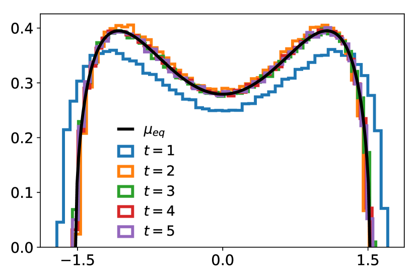
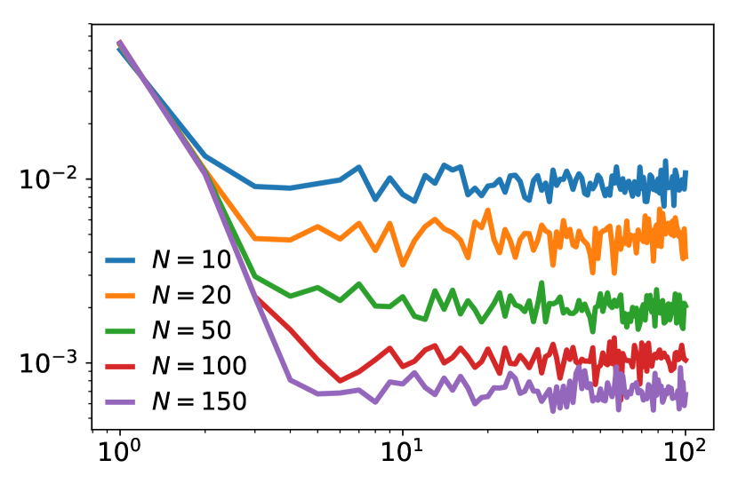
We study sampling algorithms for β𝛽\beta-ensembles with time complexity less than cubic in the cardinality of the ensemble. Following Dumitriu & Edelman (2002), we see the ensemble as the eigenvalues of a random tridiagonal matrix, namely a random Jacobi matrix. First, we provide a unifying and elementary treatment of the tridiagonal models associated to the three classical Hermite, Laguerre and Jacobi ensembles. For this purpose, we use simple changes of variables between successive reparametrizations of the coefficients defining the tridiagonal matrix. Second, we derive an approximate sampler for the simulation of β𝛽\beta-ensembles, and illustrate how fast it can be for polynomial potentials. This method combines a Gibbs sampler on Jacobi matrices and the diagonalization of these matrices. In practice, even for large ensembles, only a few Gibbs passes suffice for the marginal distribution of the eigenvalues to fit the expected theoretical distribution. When the conditionals in the Gibbs sampler can be simulated exactly, the same fast empirical convergence is observed for the fluctuations of the largest eigenvalue. Our experimental results support a conjecture by Krishnapur et al. (2016), that the Gibbs chain on Jacobi matrices of size N𝑁N mixes in 𝒪(logN)𝒪𝑁\mathcal{O}(\log N).

keywords:
β𝛽\beta-ensembles, tridiagonal random matrices, orthogonal polynomials, Gibbs sampling.
MSC 2010 subject classifications: Primary: 60K35; secondary: 65C40, 60B20, 33C45
\startlocaldefs\endlocaldefs\WarningFilter

biblatexPatching footnotes failed \WarningFilterbiblatexAttempt to redefine deprecated \WarningFilterlatexMarginpar on page \WarningFilterlatexfontFont shape \WarningFilterlatexfontSome font \WarningFilterlatexfontSize substitutions \WarningFilterbiblatexPatching footnotes failed \WarningFilterbiblatexAttempt to redefine deprecated \WarningFilterlatexMarginpar on page \WarningFilterlatexfontFont shape \WarningFilterlatexfontSome font \WarningFilterlatexfontSize substitutions \foreach\xin a,…,z \foreach\xin A,…,Z \foreach\x/\yin alpha/α, beta/β, gamma/γ, delta/δ, epsilon/ϵ, zeta/ζ, eta/η, theta/θ, iota/ι, kappa/κ, lambda/λ, mu/μ, nu/ν, xi/ξ, pi/π, rho/ρ, sigma/σ, tau/τ, upsilon/υ, phi/ϕ, chi/χ, psi/ψ, omega/ω

and

1 Introduction

β𝛽\beta-ensembles are probability distributions of the form

|Δ(x1,,xN)|βZ1n=1NeV(xn)dxn,x1,,xN\bbR,superscriptΔsubscript𝑥1subscript𝑥𝑁𝛽superscript𝑍1superscriptsubscriptproduct𝑛1𝑁superscript𝑒𝑉subscript𝑥𝑛dsubscript𝑥𝑛subscript𝑥1subscript𝑥𝑁\bbR\mathopen{}\mathclose{{}\left|\Delta(x_{1},\dots,x_{N})}\right|^{\beta}~{}Z^{-1}\prod_{n=1}^{N}e^{-V(x_{n})}\mathrm{d}x_{n},\quad x_{1},\dots,x_{N}\in\bbR, (1.1)

where Δ(x1,,xN)=i<j(xjxi)Δsubscript𝑥1subscript𝑥𝑁subscriptproduct𝑖𝑗subscript𝑥𝑗subscript𝑥𝑖\Delta(x_{1},\dots,x_{N})=\prod_{i<j}(x_{j}-x_{i}) is the Vandermonde determinant, β>0𝛽0\beta>0 is akin to an inverse temperature in statistical physics, and V:\bbR\bbR:𝑉\bbR\bbRV:\bbR\rightarrow\bbR is called the potential. Loosely speaking, one can think of (1.1) as representing the position of N𝑁N particles living on the real line, confined by the potential V𝑉V, and repelling each other through the Vandermonde determinant. As this interpretation suggests, β𝛽\beta-ensembles arise as models in statistical physics (Forrester, 2010, Chapters 1 to 3). They are also famous as the distribution of the eigenvalues of some of the classical models of random matrices. The particular values β{1,2,4}𝛽124\beta\in\{1,2,4\} respectively appear when considering specific random matrices with real, complex, or quaternionic Gaussian entries; see e.g., Forrester (2010) again or Anderson, Guionnet, and Zeitouni (2009, Chapter 4).

The case β=2𝛽2\beta=2 is of particular interest, since the distribution of {x1,,xN}subscript𝑥1subscript𝑥𝑁\{x_{1},\dots,x_{N}\} then becomes a particular determinantal point process (DPP), called an orthogonal polynomial ensemble (OPE, König, 2004). Originally introduced as models in fermionic optics by Macchi (1975), DPPs are comparatively easier to analyze than other repulsive distributions. Moreover, there exists a generic algorithm to sample from DPPs (Hough et al., 2006). Together with their analytic tractability, the existence of sampling algorithms has sparked the study of Monte Carlo integration using an OPE for the quadrature nodes (Bardenet and Hardy, 2019; Gautier, Bardenet, and Valko, 2019a; Belhadji, Bardenet, and Chainais, 2019).

Besides Monte Carlo integration, numerical procedures to generate samples from β𝛽\beta-ensembles are also needed to establish conjectures in statistical physics or random matrix theory. For instance, using a tailored version of the generic DPP sampler of Hough et al. (2006), Olver et al. (2014) explore so-called universality properties in random matrix theory, and make conjectures on the law of maxxisubscript𝑥𝑖\max x_{i} when β=2𝛽2\beta=2 and V𝑉V is a polynomial of degree 444. Chafaï & Ferré (2018) rather use Hamiltonian Monte Carlo to approximately sample from various Coulomb gases, including (1.1) with β=2𝛽2\beta=2 and V(x)=x4/4𝑉𝑥superscript𝑥44V(x)=x^{4}/4, and investigate their limiting features when N𝑁N\rightarrow\infty. From a different perspective, Li & Menon (2013) view (1.1) as the equilibrium distribution for the Dyson Brownian motion associated to the potential V𝑉V. When β=2𝛽2\beta=2, they generate approximate samples by discretizing the corresponding stochastic differential equation.

Algorithms to sample from β𝛽\beta-ensembles come in three different guises, which we describe in increasing order of complexity. First, when β>0𝛽0\beta>0 and V𝑉V is the negative logarithm of a Gaussian, gamma, or beta pdf, we speak of the Hermite, Laguerre, and Jacobi β𝛽\beta-ensemble, respectively. Dumitriu & Edelman (2002) showed that the Hermite and Laguerre β𝛽\beta-ensembles can be characterized as the eigenvalue distribution of a random tridiagonal matrix with easy-to-sample independent entries. This gives a \calO(N2)\calOsuperscript𝑁2\calO(N^{2}) sampling algorithm. Dumitriu & Edelman (2002) expected the same to hold for the Jacobi β𝛽\beta-ensemble, which was later proved by Killip & Nenciu (2004).

Second, when β=2𝛽2\beta=2, the generic projection DPP sampler of Hough et al. (2006) applies. That there actually exists an exact sampler is maybe surprising, and it is a particular feature of DPPs among interacting particle systems. The procedure remains costly, though. It has at least a cubic cost in N𝑁N, with the total cost further depending on rejection sampling subroutines, the cost of which is case-dependent and has been left uninvestigated. Additionally, it is required in this procedure to numerically evaluate the first N𝑁N orthonormal polynomials pk,k=0,,N1formulae-sequencesubscript𝑝𝑘𝑘0𝑁1p_{k},k=0,\dots,N-1 with respect to eV(x)dxsuperscript𝑒𝑉𝑥d𝑥e^{-V(x)}\mathrm{d}x. This is traditionally done using their recurrence relation

bk1pk1(x)+akpk(x)+bkpk+1(x)=xpk(x),subscript𝑏𝑘1subscript𝑝𝑘1𝑥subscript𝑎𝑘subscript𝑝𝑘𝑥subscript𝑏𝑘subscript𝑝𝑘1𝑥𝑥subscript𝑝𝑘𝑥\sqrt{b_{k-1}}p_{k-1}(x)+a_{k}p_{k}(x)+\sqrt{b_{k}}p_{k+1}(x)=xp_{k}(x), (1.2)

see e.g., Gautschi (2004). In the Hermite, Laguerre, and Jacobi case, the recurrence coefficients ak,bksubscript𝑎𝑘subscript𝑏𝑘a_{k},b_{k} are known, but as we just saw, these three cases are already covered by a computationally more efficient tridiagonal matrix model. When the coefficients in (1.2) are not known, one can either rely on the Stieltjes algorithm (Gautschi, 2004, Section 2.2) or numerically solve a Riemann-Hilbert problem (Olver, 2011). The latter is theoretically only an \calO(N)\calO𝑁\calO(N) overcost.

A third algorithm is Markov chain Monte Carlo (MCMC, see e.g., Robert & Casella, 2004), which is in principle valid for any β>0𝛽0\beta>0 and any V𝑉V that gives a well-defined distribution in (1.1). MCMC only requires to evaluate the pdf in (1.1) pointwise and up to a constant, but it only delivers approximate samples of (1.1), in the sense that it outputs a sample from a Markov chain with (1.1) as its limiting distribution. The issue is that the performance of MCMC samplers – the mixing time of the Markov chain – deteriorates when N1much-greater-than𝑁1N\gg 1, which is typically the regime of interest for conjectures in random matrix theory or statistical physics. Hybric Monte Carlo (HMC, Duane et al., 1987; Neal, 2011) is an MCMC sampler that has demonstrated good mixing in high-dimensional problems, provided one can evaluate the gradient of the pdf in (1.1). For β𝛽\beta-ensembles with β=2𝛽2\beta=2, Chafaï & Ferré (2018) provide empirical evidence that the output of HMC successfully reproduces known limiting features of the large N𝑁N regime, and they raise new conjectures. The main limitation of this approach is the large number of MCMC iterations required by HMC: Chafaï & Ferré (2018) require at least 104superscript10410^{4} iterations and are restricted to N50𝑁50N\leq 50.

In this paper, we further investigate fast samplers of β𝛽\beta-ensembles. Our contributions are twofold. First we gather existing tools from different communities to give an elementary proof of the tridiagonal models for the Hermite, Laguerre, and Jacobi β𝛽\beta-ensembles. This proof crucially relies on successive reparametrizations of the recurrence coefficients in (1.2) and unifies the treatment of tridiagonal models for the three classical β𝛽\beta-ensembles, pioneered with two different methods by Dumitriu & Edelman (2002) and Killip & Nenciu (2004). We take no credit for the originality of the proof: the credit should go – among others cited below – to Dette & Nagel (2012), who studied distributions on the space of moments, and recognized these three β𝛽\beta-ensembles as corresponding to natural distributions over moments. We rather take credit for a stand-alone and elementary version of this unifying proof, using only basic facts on orthogonal polynomials and linear algebra.

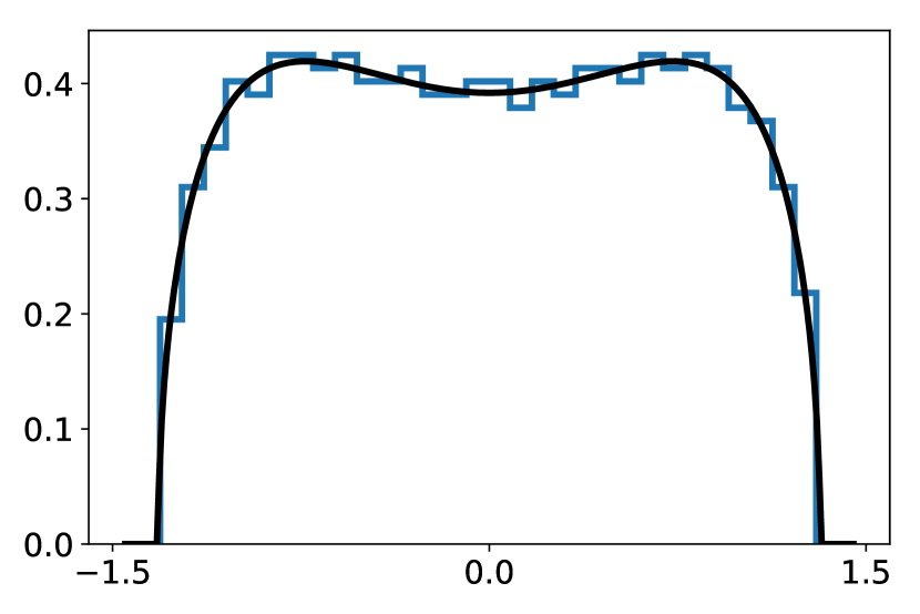
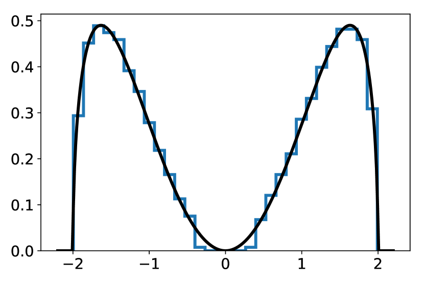
Our second contribution is an MCMC sampler that applies to polynomial potentials. For V𝑉V of degree at most 6, we give experimental evidence that the resulting Markov chain mixes extremely fast, which confirms an intuition of Krishnapur et al. (2016, Section 2). On a variety of potentials, we demonstrate that our simple Gibbs Markov kernel yields a much cheaper (although approximate) sampler than the exact procedure of Hough et al. (2006, for β=2𝛽2\beta=2). Importantly, our Markov kernel outperforms the HMC approach of Chafaï & Ferré (2018) in the particular case of β𝛽\beta-ensembles. To give an idea, we are able to reproduce known features of (1.1) for values of N𝑁N in the hundreds, using only a few Gibbs sweeps, totaling a few seconds on a modern laptop: it takes roughly 101010s for N=200𝑁200N=200 points and less than a minute for N=1000𝑁1000N=1000 points. That such a basic Gibbs kernel can outperform HMC may seem surprising. The key is that we exploit the structure of β𝛽\beta-ensembles by defining a Markov chain on the recurrence coefficients of orthogonal polynomials. These recurrence coefficients are defined similarly to (1.2), but this time using the orthogonal polynomials with respect to a random discrete measure, the support of which is the β𝛽\beta-ensemble. Intuitively, in that new parametrization, the interaction between variables is short-range compared to the interaction among particles in (1.1), and Gibbs sampling thus becomes easier. In this sense, our MCMC kernel extends the tridiagonal models of the three classical β𝛽\beta-ensembles. Finally, we note that all experiments can be reproduced using our DPPy  toolbox (Gautier, Polito, Bardenet, and Valko, 2019b, https://github.com/guilgautier/DPPy), which features all samplers described here.

The rest of the paper is organized as follows. In Section 2, we survey existing results on tridiagonal models for β𝛽\beta-ensembles. Known exact sampling results actually take the form of diagonalizing random Jacobi matrices, that is, tridiagonal matrices whose coefficients are the recurrence coefficients of a sequence of orthogonal polynomials. We introduce the necessary background on orthogonal polynomials in Section 3. In Section 4, we perform the change of variables between the points of a β𝛽\beta-ensemble augmented with weights and the entries of a Jacobi matrix. In Section 5, we give an elementary proof of the known results on tridiagonal models. Finally, in Section 6, we demonstrate a simple MCMC scheme based on a Gibbs kernel, to sample Jacobi matrices corresponding to β𝛽\beta-ensembles with polynomial potentials.

2 Classical β𝛽\beta-ensembles and their tridiagonal models

The Hermite, Laguerre and Jacobi β𝛽\beta-ensembles were originally defined for β{1,2,4}𝛽124\beta\in\mathopen{}\mathclose{{}\left\{1,2,4}\right\}, as the eigenvalue distribution of some random full matrices; see e.g., Anderson et al. (2009). The latter matrices are symmetrizations of matrices filled with i.i.d. real, complex, or quarternionic Gaussian variables when β𝛽\beta is respectively 1,2,121,2, and 444. In this section, we recall the seminal results of Dumitriu & Edelman (2002) and Killip & Nenciu (2004) regarding the construction of real-symmetric tridiagonal random matrices, whose eigenvalues follow the classical Hermite, Laguerre and Jacobi β𝛽\beta-ensembles. These results actually allow any β(0,+)𝛽0\beta\in(0,+\infty), and can be interpreted as samplers with \calO(N2)\calOsuperscript𝑁2\calO(N^{2}) time complexity, by simply diagonalizing the proposed tridiagonal matrices.

We note \bfa(a1,,aN)N\bfasubscript𝑎1subscript𝑎𝑁superscript𝑁\bfa\triangleq\mathopen{}\mathclose{{}\left(a_{1},\dots,a_{N}}\right)\in\mathbb{R}^{N}, \bfb(b1,,bN1)(0,+)N1\bfbsubscript𝑏1subscript𝑏𝑁1superscript0𝑁1\bfb\triangleq\mathopen{}\mathclose{{}\left(b_{1},\dots,b_{N-1}}\right)\in(0,+\infty)^{N-1}, and define the tridiagonal matrix

J𝐚,𝐛[a1b1(0)b1a2bN1(0)bN1aN].subscript𝐽𝐚𝐛matrixsubscript𝑎1subscript𝑏1missing-subexpression0subscript𝑏1subscript𝑎2missing-subexpressionmissing-subexpressionsubscript𝑏𝑁10missing-subexpressionsubscript𝑏𝑁1subscript𝑎𝑁J_{\mathbf{a},\mathbf{b}}\triangleq\begin{bmatrix}a_{1}&\sqrt{b_{1}}&&(0)\\ \sqrt{b_{1}}&a_{2}&\ddots&\\ &\ddots&\ddots&\sqrt{b_{N-1}}\\ (0)&&\sqrt{b_{N-1}}&a_{N}\end{bmatrix}.\\ (2.1)

Such a matrix is called a Jacobi matrix. As we will see in Section 3, Jacobi matrices naturally arise in the study of orthogonal polynomials.

To build the random tridiagonal matrix model for the Hermite β𝛽\beta-ensemble, Dumitriu & Edelman (2002) started from to the original random full matrix model defining the Hermite ensemble with β=1𝛽1\beta=1. More specifically, they considered the symmetric part of a random matrix filled with i.i.d. unit Gaussians, and applied Householder transformations to reduce it to tridiagonal form, as in, e.g., Golub & Van Loan (2013, Section 5.4.8).

Theorem 2.1 (Dumitriu & Edelman, 2002, II C, for μ=0𝜇0\mu=0 and σ=1𝜎1\sigma=1).

The Hermite β𝛽\beta-ensemble, defined as (1.1) with potential V(x)=12σ2(xμ)2𝑉𝑥12superscript𝜎2superscript𝑥𝜇2V(x)=\frac{1}{2\sigma^{2}}(x-\mu)^{2}, corresponds to the eigenvalue distribution of the tridiagonal matrix J\bfa,\bfbsubscript𝐽\bfa\bfbJ_{\bfa,\bfb} in (2.1), with entries drawn independently as

an\calN(μ,σ2),andbnΓ(β2(Nn),σ2).formulae-sequencesimilar-tosubscript𝑎𝑛\calN𝜇superscript𝜎2andsimilar-tosubscript𝑏𝑛Γ𝛽2𝑁𝑛superscript𝜎2a_{n}\sim\calN\mathopen{}\mathclose{{}\left(\mu,\sigma^{2}}\right),\quad\text{and}\quad b_{n}\sim\Gamma\mathopen{}\mathclose{{}\left(\frac{\beta}{2}(N-n),\sigma^{2}}\right). (2.2)

For the Laguerre β𝛽\beta-ensemble, Dumitriu & Edelman (2002) used the same linear algebra techniques starting from the original full matrix model defining the Laguerre β𝛽\beta-ensemble for β=1𝛽1\beta=1. The latter corresponds to the eigenvalue distribution of the covariance matrix XX𝖳𝑋superscript𝑋𝖳XX^{\mathsf{\scriptscriptstyle T}} of i.i.d. \calN(0,I)\calN0𝐼\calN\mathopen{}\mathclose{{}\left(0,I}\right) vectors. More specifically, they reduced the matrix X𝑋X to bidiagonal form, see, e.g., Golub & Van Loan (2013, Section 8.3.1).

Theorem 2.2 (Dumitriu & Edelman, 2002, III B, for k=β2(MN+1)𝑘𝛽2𝑀𝑁1k=\frac{\beta}{2}(M-N+1) and θ=2𝜃2\theta=2).


The Laguerre β𝛽\beta-ensemble, defined as (1.1) with potential V(x)=(k1)log(x)+xθ𝑉𝑥𝑘1𝑥𝑥𝜃V(x)=-(k-1)\log(x)+\frac{x}{\theta}, corresponds to the eigenvalue distribution of the tridiagonal matrix J\bfa,\bfbsubscript𝐽\bfa\bfbJ_{\bfa,\bfb} in (2.1) parametrized by

a1=ξ1,andan=ξ2n2+ξ2n1,for 2nN,andformulae-sequenceformulae-sequencesubscript𝑎1subscript𝜉1andformulae-sequencesubscript𝑎𝑛subscript𝜉2𝑛2subscript𝜉2𝑛1for 2𝑛𝑁and\displaystyle a_{1}=\xi_{1},\quad\text{and}\quad a_{n}=\xi_{2n-2}+\xi_{2n-1},\quad\text{for }2\leq n\leq N,\quad\text{and} (2.3)
bn=ξ2n1ξ2n,for 1nN1,formulae-sequencesubscript𝑏𝑛subscript𝜉2𝑛1subscript𝜉2𝑛for 1𝑛𝑁1\displaystyle b_{n}=\xi_{2n-1}\xi_{2n},\quad\text{for }1\leq n\leq N-1,

with independent coefficients

ξ2n1subscript𝜉2𝑛1\displaystyle\xi_{2n-1} Γ(β2(Nn)+k,θ),andξ2nsimilar-toabsentΓ𝛽2𝑁𝑛𝑘𝜃andsubscript𝜉2𝑛\displaystyle\sim\Gamma\mathopen{}\mathclose{{}\left(\frac{\beta}{2}(N-n)+k,\theta}\right),\quad\text{and}\quad\xi_{2n} Γ(β2(Nn),θ).similar-toabsentΓ𝛽2𝑁𝑛𝜃\displaystyle\sim\Gamma\mathopen{}\mathclose{{}\left(\frac{\beta}{2}(N-n),\theta}\right). (2.4)

Dumitriu & Edelman (2002) left the construction of a tridiagonal model for the Jacobi β𝛽\beta-ensemble as an open problem. Killip & Nenciu (2004) found such a model as a byproduct of their study the Circular β𝛽\beta-ensemble. The latter ensemble is originally defined, for β{1,2,4}𝛽124\beta\in\mathopen{}\mathclose{{}\left\{1,2,4}\right\}, as the eigenvalue distribution of orthogonal, unitary and symplectic matrices drawn uniformly at random from the corresponding Haar measures. First, Killip & Nenciu (2004) applied Householder transformations to reduce to quindiagonal form a unitary matrix drawn uniformly at random. Second, they projected the resulting eigenvalues onto the real line to obtain the tridiagonal model for the Jacobi β𝛽\beta-ensemble.

Theorem 2.3 (Killip & Nenciu, 2004, Theorem 2).

The Jacobi β𝛽\beta-ensemble, defined as (1.1) with potential V(x)=[(a1)log(x)+(b1)log(1x)]𝑉𝑥delimited-[]𝑎1𝑥𝑏11𝑥V(x)=-[(a-1)\log(x)+(b-1)\log(1-x)], corresponds to the eigenvalue distribution of the tridiagonal matrix J\bfa,\bfbsubscript𝐽\bfa\bfbJ_{\bfa,\bfb} in (2.1) parametrized by

a1subscript𝑎1\displaystyle a_{1} =c1,absentsubscript𝑐1\displaystyle=c_{1}, an=(1c2n3)c2n2+(1c2n2)c2n1,for 2nN,formulae-sequencesubscript𝑎𝑛1subscript𝑐2𝑛3subscript𝑐2𝑛21subscript𝑐2𝑛2subscript𝑐2𝑛1for 2𝑛𝑁\displaystyle a_{n}=(1-c_{2n-3})c_{2n-2}+(1-c_{2n-2})c_{2n-1},\quad\text{for }2\leq n\leq N, (2.5)
b1subscript𝑏1\displaystyle b_{1} =c1(1c1)c2,absentsubscript𝑐11subscript𝑐1subscript𝑐2\displaystyle=c_{1}(1-c_{1})c_{2}, bn=(1c2n2)c2n1(1c2n1)c2n,for 2nN1,formulae-sequencesubscript𝑏𝑛1subscript𝑐2𝑛2subscript𝑐2𝑛11subscript𝑐2𝑛1subscript𝑐2𝑛for 2𝑛𝑁1\displaystyle b_{n}=(1-c_{2n-2})c_{2n-1}(1-c_{2n-1})c_{2n},\quad\text{for }2\leq n\leq N-1,

with independent coefficients

c2n1subscript𝑐2𝑛1\displaystyle c_{2n-1} Beta(β2(Nn)+a,β2(Nn)+b),andsimilar-toabsentBeta𝛽2𝑁𝑛𝑎𝛽2𝑁𝑛𝑏and\displaystyle\sim\operatorname{Beta}\mathopen{}\mathclose{{}\left(\frac{\beta}{2}(N-n)+a,\frac{\beta}{2}(N-n)+b}\right),\quad\text{and} (2.6)
c2nsubscript𝑐2𝑛\displaystyle c_{2n} Beta(β2(Nn),β2(Nn1)+a+b).similar-toabsentBeta𝛽2𝑁𝑛𝛽2𝑁𝑛1𝑎𝑏\displaystyle\sim\operatorname{Beta}\mathopen{}\mathclose{{}\left(\frac{\beta}{2}(N-n),\frac{\beta}{2}(N-n-1)+a+b}\right).

Observe how the stars align for these three special β𝛽\beta-ensembles: Hermite, Laguerre, and Jacobi. The coefficients in successive parameterizations of the Jacobi matrix J𝐚,𝐛subscript𝐽𝐚𝐛J_{\mathbf{a},\mathbf{b}} are independent with easy-to-sample distributions. From a practical point of view, for any β>0𝛽0\beta>0, the computation of the eigenvalues of these random real-symmetric tridiagonal matrices can be seen as a 𝒪(N2)𝒪superscript𝑁2\mathcal{O}(N^{2}) sampler for each of the model; see Coakley & Rokhlin (2013) for practical approaches to diagonalizing such matrices that can even run in quasi-linear time.

Studying distributions over the space of moments, Dette & Nagel (2012) elegantly derived the three classical tridiagonal models as the supports of random atomic measures corresponding to natural moment distributions. On our side, we provide a unified treatment of these three classical models using a more pedestrian, sampling-motivated approach. To do this, we consider an atomic measure μ=n=1Nωnδxn𝜇superscriptsubscript𝑛1𝑁subscript𝜔𝑛subscript𝛿subscript𝑥𝑛\mu=\sum_{n=1}^{N}\omega_{n}\delta_{x_{n}}, whose support points are distributed as a target β𝛽\beta-ensemble, and take the Jacobi matrix J𝐚,𝐛subscript𝐽𝐚𝐛J_{\mathbf{a},\mathbf{b}} in (2.1) with coefficients the recurrence coefficients (1.2) of the orthonormal polynomials w.r.t. μ𝜇\mu. We shall see in Section 3 that the recurrence coefficients are a suitable reparametrization of the atomic measure μ𝜇\mu. In particular, the support of μ𝜇\mu actually coincides with the eigenvalues of J𝐚,𝐛subscript𝐽𝐚𝐛J_{\mathbf{a},\mathbf{b}}, so that a tridiagonal model for the support of μ𝜇\mu follows from knowing how to randomize J𝐚,𝐛subscript𝐽𝐚𝐛J_{\mathbf{a},\mathbf{b}}.

The first step of our proof will be to rederive Theorem 2.4, which allows changing variables from the nodes and weights of an atomic measure μ𝜇\mu to the recurrence coefficients defining the Jacobi matrix J𝐚,𝐛subscript𝐽𝐚𝐛J_{\mathbf{a},\mathbf{b}}. Note that the specific choice of distribution on the weights is simply of mathematical convenience.

Theorem 2.4 (Krishnapur et al., 2016, Proposition 2).

Consider a random atomic measure μ=n=1Nωnδxn𝜇superscriptsubscript𝑛1𝑁subscript𝜔𝑛subscript𝛿subscript𝑥𝑛\mu=\sum_{n=1}^{N}\omega_{n}\delta_{x_{n}}, with nodes and weights independently distributed according to a β𝛽\beta-ensemble with potential V𝑉V (1.1) and a Dirichlet Dir(β/2)Dir𝛽2\operatorname{Dir}\mathopen{}\mathclose{{}\left(\beta/2}\right), respectively. Otherly put, the joint distribution of (x1,,xN,w1,,wN)subscript𝑥1subscript𝑥𝑁subscript𝑤1subscript𝑤𝑁(x_{1},\dots,x_{N},w_{1},\dots,w_{N}) is proportional to

|Δ(x1,,xN)|βen=1NV(xn)dx1:Nn=1Nwnβ21𝟙wn0𝟙n=1Nwn=1dw1:N1.superscriptΔsubscript𝑥1subscript𝑥𝑁𝛽superscriptesuperscriptsubscript𝑛1𝑁𝑉subscript𝑥𝑛dsubscript𝑥:1𝑁superscriptsubscriptproduct𝑛1𝑁superscriptsubscript𝑤𝑛𝛽21subscript1subscript𝑤𝑛0subscript1superscriptsubscript𝑛1𝑁subscript𝑤𝑛1dsubscript𝑤:1𝑁1\mathopen{}\mathclose{{}\left|\Delta\mathopen{}\mathclose{{}\left(x_{1},\dots,x_{N}}\right)}\right|^{\beta}\operatorname{\mathrm{e}}^{-\sum\limits_{n=1}^{N}V(x_{n})}\mathrm{d}x_{1:N}\prod_{n=1}^{N}w_{n}^{\frac{\beta}{2}-1}\mathds{1}_{w_{n}\geq 0}\mathds{1}_{\sum_{n=1}^{N}w_{n}=1}\mathrm{d}w_{1:N-1}. (2.7)

Then, the recurrence coefficients (a1,,aN,b1,,bN1)subscript𝑎1subscript𝑎𝑁subscript𝑏1subscript𝑏𝑁1(a_{1},\dots,a_{N},b_{1},\dots,b_{N-1}) of μ𝜇\mu have joint distribution proportional to

n=1N1bnβ2(Nn)1eTr[V(J𝐚,𝐛)]da1:Ndb1:N1.superscriptsubscriptproduct𝑛1𝑁1superscriptsubscript𝑏𝑛𝛽2𝑁𝑛1superscripteTr𝑉subscript𝐽𝐚𝐛dsubscript𝑎:1𝑁dsubscript𝑏:1𝑁1\prod_{n=1}^{N-1}b_{n}^{\frac{\beta}{2}(N-n)-1}\operatorname{\mathrm{e}}^{-\operatorname{Tr}\mathopen{}\mathclose{{}\left[V(J_{\mathbf{a},\mathbf{b}})}\right]}\mathrm{d}a_{1:N}\mathrm{d}b_{1:N-1}. (2.8)

In Section 4, we first re-prove that the change of variables underlying Theorem 2.4 is valid. Then, in Section 5, we obtain the three classical tridiagonal models of Theorems 2.1, 2.2, and 2.3 as instances of this result, using further smart-but-simple changes of variables. Before delving into the proof, we first survey how Jacobi matrices naturally appear in the theory of orthogonal polynomials.

3 Atomic measures, moments and Jacobi matrices

Throughout this section, we let μ=n=1Nwnδxn𝜇superscriptsubscript𝑛1𝑁subscript𝑤𝑛subscript𝛿subscript𝑥𝑛\mu=\sum_{n=1}^{N}w_{n}\delta_{x_{n}} be a discrete probability measure on \bbR\bbR\bbR with N𝑁N distinct atoms x1,,xNsubscript𝑥1subscript𝑥𝑁x_{1},\dots,x_{N} and positive weights ω1,,ωNsubscript𝜔1subscript𝜔𝑁\omega_{1},\dots,\omega_{N}. We further denote its moments by

mkn=1Nwnxnk,k0.formulae-sequencesubscript𝑚𝑘superscriptsubscript𝑛1𝑁subscript𝑤𝑛superscriptsubscript𝑥𝑛𝑘𝑘0m_{k}\triangleq\sum_{n=1}^{N}w_{n}x_{n}^{k},\quad k\geq 0.

3.1 Orthogonal polynomials and Jacobi matrices

This section closely follows Simon (2011, Section 1.3), to which we refer for details. Applying the Gram-Schmidt procedure in L2(μ)superscript𝐿2𝜇L^{2}(\mu) to the monomials (xxk)k=0N1superscriptsubscriptmaps-to𝑥superscript𝑥𝑘𝑘0𝑁1(x\mapsto x^{k})_{k=0}^{N-1} yields monic polynomials (Pk)k=0N1superscriptsubscriptsubscript𝑃𝑘𝑘0𝑁1(P_{k})_{k=0}^{N-1} with degPk=kdegreesubscript𝑃𝑘𝑘\deg P_{k}=k and

Pk,Pμn=1NwnPk(xn)P(xn)=0,k.formulae-sequencesubscriptsubscript𝑃𝑘subscript𝑃𝜇superscriptsubscript𝑛1𝑁subscript𝑤𝑛subscript𝑃𝑘subscript𝑥𝑛subscript𝑃subscript𝑥𝑛0𝑘\mathopen{}\mathclose{{}\left\langle P_{k},P_{\ell}}\right\rangle_{\mu}\triangleq\sum_{n=1}^{N}w_{n}P_{k}(x_{n})P_{\ell}(x_{n})=0,\quad k\neq\ell. (3.1)

These polynomials are called the monic orthogonal polynomials (monic OPs, in short) with respect to μ𝜇\mu. We define the N𝑁N-th monic OP as

PN(x)=n=1N(xxn).subscript𝑃𝑁𝑥superscriptsubscriptproduct𝑛1𝑁𝑥subscript𝑥𝑛P_{N}(x)=\prod_{n=1}^{N}(x-x_{n}).

Since PNμPN,PNμ=0subscriptnormsubscript𝑃𝑁𝜇subscriptsubscript𝑃𝑁subscript𝑃𝑁𝜇0\|P_{N}\|_{\mu}\triangleq\mathopen{}\mathclose{{}\left\langle P_{N},P_{N}}\right\rangle_{\mu}=0, PNsubscript𝑃𝑁P_{N} is the zero vector of L2(μ)superscript𝐿2𝜇L^{2}(\mu): it is orthogonal to all Pksubscript𝑃𝑘P_{k} with kN1𝑘𝑁1k\leq N-1.

Furthermore, for any n<N𝑛𝑁n<N, since xPn,Pkμ=Pn,xPkμ=0subscript𝑥subscript𝑃𝑛subscript𝑃𝑘𝜇subscriptsubscript𝑃𝑛𝑥subscript𝑃𝑘𝜇0\mathopen{}\mathclose{{}\left\langle xP_{n},P_{k}}\right\rangle_{\mu}=\mathopen{}\mathclose{{}\left\langle P_{n},xP_{k}}\right\rangle_{\mu}=0 for k<n1𝑘𝑛1k<n-1, the polynomial xPn𝑥subscript𝑃𝑛xP_{n} can be uniquely expressed using only Pn1subscript𝑃𝑛1P_{n-1}, Pnsubscript𝑃𝑛P_{n} and Pn+1subscript𝑃𝑛1P_{n+1}. This is usually phrased as follows. The monic OPs satisfy a three-term recurrence relation involving two sequences of recurrence coefficients, namely

P10,P01 andxPn(x)=bnPn1(x)+an+1Pn(x)+Pn+1(x),0n<N,missing-subexpressionformulae-sequencesubscript𝑃10subscript𝑃01 andmissing-subexpressionformulae-sequence𝑥subscript𝑃𝑛𝑥subscript𝑏𝑛subscript𝑃𝑛1𝑥subscript𝑎𝑛1subscript𝑃𝑛𝑥subscript𝑃𝑛1𝑥for-all0𝑛𝑁\displaystyle\begin{aligned} &P_{-1}\equiv 0,P_{0}\equiv 1\text{ and}\\ &xP_{n}(x)=b_{n}P_{n-1}(x)+a_{n+1}P_{n}(x)+P_{n+1}(x),\quad\forall 0\leq n<N,\end{aligned} (3.2)

where \bfa=a1:N=(an)N\bfasubscript𝑎:1𝑁subscript𝑎𝑛superscript𝑁\bfa=a_{1:N}=\mathopen{}\mathclose{{}\left(a_{n}}\right)\in\mathbb{R}^{N}, and \bfb=b1:N1=(bn)(0,+)N1\bfbsubscript𝑏:1𝑁1subscript𝑏𝑛superscript0𝑁1\bfb=b_{1:N-1}=\mathopen{}\mathclose{{}\left(b_{n}}\right)\in(0,+\infty)^{N-1}. These relations can be written in matrix form as

[a11(0)b1a21(0)bN1aN][P0(x)PN2(x)PN1(x)]=x[P0(x)PN2(x)PN1(x)][00PN(x)].matrixsubscript𝑎11missing-subexpression0subscript𝑏1subscript𝑎2missing-subexpressionmissing-subexpression10missing-subexpressionsubscript𝑏𝑁1subscript𝑎𝑁matrixsubscript𝑃0𝑥subscript𝑃𝑁2𝑥subscript𝑃𝑁1𝑥𝑥matrixsubscript𝑃0𝑥subscript𝑃𝑁2𝑥subscript𝑃𝑁1𝑥matrix00subscript𝑃𝑁𝑥\begin{bmatrix}a_{1}&1&&(0)\\ b_{1}&a_{2}&\ddots&\\ &\ddots&\ddots&1\\ (0)&&b_{N-1}&a_{N}\end{bmatrix}\begin{bmatrix}P_{0}(x)\\ \vdots\\ P_{N-2}(x)\\ P_{N-1}(x)\end{bmatrix}=x\begin{bmatrix}P_{0}(x)\\ \vdots\\ P_{N-2}(x)\\ P_{N-1}(x)\end{bmatrix}-\begin{bmatrix}0\\ \vdots\\ 0\\ P_{N}(x)\end{bmatrix}. (3.3)

From (3.3), it is clear that the roots of PNsubscript𝑃𝑁P_{N} are also eigenvalues of the tridiagonal matrix T𝐚,𝐛subscript𝑇𝐚𝐛T_{\mathbf{a},\mathbf{b}} appearing on the left-hand side. Roots and eigenvalues actually coincide since PNsubscript𝑃𝑁P_{N} has N𝑁N distinct roots by definition.

A lot more can be said on the links between OPs and their recurrence coefficients. For instance, Proposition 3.1 will be of use later on.

Proposition 3.1.

The squared norms of the monic polynomials (Pn)n=0N1superscriptsubscriptsubscript𝑃𝑛𝑛0𝑁1(P_{n})_{n=0}^{N-1} can be expressed as

P0μ2=1,Pkμ2=n=1kbn,1kN1.formulae-sequencesuperscriptsubscriptnormsubscript𝑃0𝜇21formulae-sequencesuperscriptsubscriptnormsubscript𝑃𝑘𝜇2superscriptsubscriptproduct𝑛1𝑘subscript𝑏𝑛for-all1𝑘𝑁1\mathopen{}\mathclose{{}\left\|P_{0}}\right\|_{\mu}^{2}=1,\quad\mathopen{}\mathclose{{}\left\|P_{k}}\right\|_{\mu}^{2}=\prod_{n=1}^{k}b_{n},\quad\forall 1\leq k\leq N-1. (3.4)
Proof.

For k=0𝑘0k=0, P0μ2=n=1Nwn=1superscriptsubscriptnormsubscript𝑃0𝜇2superscriptsubscript𝑛1𝑁subscript𝑤𝑛1\mathopen{}\mathclose{{}\left\|P_{0}}\right\|_{\mu}^{2}=\sum_{n=1}^{N}w_{n}=1. Then, for any 1kN11𝑘𝑁11\leq k\leq N-1,

(3.2),Pk1μsubscriptitalic-(3.2italic-)subscript𝑃𝑘1𝜇\displaystyle\mathopen{}\mathclose{{}\left\langle\eqref{eq:3-terms_recurrence_monic_orthogonal_poly},P_{k-1}}\right\rangle_{\mu} xPk,Pk1μ=bkPk1,Pk1μabsentsubscript𝑥subscript𝑃𝑘subscript𝑃𝑘1𝜇subscriptsubscript𝑏𝑘subscript𝑃𝑘1subscript𝑃𝑘1𝜇\displaystyle\Longleftrightarrow\mathopen{}\mathclose{{}\left\langle xP_{k},P_{k-1}}\right\rangle_{\mu}=\mathopen{}\mathclose{{}\left\langle b_{k}P_{k-1},P_{k-1}}\right\rangle_{\mu}
Pk,xPk1μ=bkPk1,Pk1μabsentsubscriptsubscript𝑃𝑘𝑥subscript𝑃𝑘1𝜇subscript𝑏𝑘subscriptsubscript𝑃𝑘1subscript𝑃𝑘1𝜇\displaystyle\Longleftrightarrow\mathopen{}\mathclose{{}\left\langle P_{k},xP_{k-1}}\right\rangle_{\mu}=b_{k}\mathopen{}\mathclose{{}\left\langle P_{k-1},P_{k-1}}\right\rangle_{\mu}
Pk,xnμ=bkPk1μ2absentsubscriptsubscript𝑃𝑘superscript𝑥𝑛𝜇subscript𝑏𝑘superscriptsubscriptnormsubscript𝑃𝑘1𝜇2\displaystyle\Longleftrightarrow\mathopen{}\mathclose{{}\left\langle P_{k},x^{n}}\right\rangle_{\mu}=b_{k}\mathopen{}\mathclose{{}\left\|P_{k-1}}\right\|_{\mu}^{2}
Pkμ2=bkPk1μ2,absentsuperscriptsubscriptnormsubscript𝑃𝑘𝜇2subscript𝑏𝑘superscriptsubscriptnormsubscript𝑃𝑘1𝜇2\displaystyle\Longleftrightarrow\mathopen{}\mathclose{{}\left\|P_{k}}\right\|_{\mu}^{2}=b_{k}\mathopen{}\mathclose{{}\left\|P_{k-1}}\right\|_{\mu}^{2},

and a simple recursion provides Pkμ2=n=1kbn>0superscriptsubscriptnormsubscript𝑃𝑘𝜇2superscriptsubscriptproduct𝑛1𝑘subscript𝑏𝑛0\mathopen{}\mathclose{{}\left\|P_{k}}\right\|_{\mu}^{2}=\prod_{n=1}^{k}b_{n}>0. ∎

Denoting by D=diag(P0,,PN1)𝐷diagnormsubscript𝑃0normsubscript𝑃𝑁1D=\operatorname{diag}\mathopen{}\mathclose{{}\left(\mathopen{}\mathclose{{}\left\|P_{0}}\right\|,\dots,\mathopen{}\mathclose{{}\left\|P_{N-1}}\right\|}\right), Proposition 3.1 yields J𝐚,𝐛=D1T𝐚,𝐛Dsubscript𝐽𝐚𝐛superscript𝐷1subscript𝑇𝐚𝐛𝐷J_{\mathbf{a},\mathbf{b}}=D^{-1}T_{\mathbf{a},\mathbf{b}}D, where we recall that the Jacobi matrix J𝐚,𝐛subscript𝐽𝐚𝐛J_{\mathbf{a},\mathbf{b}} was defined in (2.1). This yields the following proposition.

Proposition 3.2.

The atoms of μ𝜇\mu, coincide with the eigenvalues of J𝐚,𝐛subscript𝐽𝐚𝐛J_{\mathbf{a},\mathbf{b}}, where the coefficients of the matrix are taken to be the recurrence coefficients of the monic OPs with respect to μ𝜇\mu.

Proposition 3.2 already gives a tentative \calO(N2)\calOsuperscript𝑁2\calO(N^{2}) sampling algorithm for β𝛽\beta-ensembles: find a distribution over Jacobi matrices such that the eigenvalues form the desired β𝛽\beta-ensemble. This is precisely what the tridiagonal models of Dumitriu & Edelman (2002) do; see Theorem 2.1. To give a complete elementary proof, we need to perform a change of variables from the atoms and weights of μ𝜇\mu to the recurrence coefficients. The rest of this section introduces the tools needed for this change of variables, which is then performed in Section 4.

So far, we have explained how to obtain a Jacobi matrix from an atomic measure with finite support. The reverse construction is also possible and elementary. This is called Favard’s theorem for atomic measures with finite support. To save space and because our proof would be a simple copy of Simon’s book, we only give a reference. We have used the same notation as Simon throughout this section, for ease of reference.

Theorem 3.1 (Simon, 2011, Theorem 1.3.3).

Let

\bbR>N{x1,,xN\bbRx1>>xN}andSN{ω1,,ωN1>0n=1N1ωn<1}.formulae-sequencesuperscriptsubscript\bbR𝑁conditional-setsubscript𝑥1subscript𝑥𝑁\bbRsubscript𝑥1subscript𝑥𝑁andsubscript𝑆𝑁conditional-setsubscript𝜔1subscript𝜔𝑁10superscriptsubscript𝑛1𝑁1subscript𝜔𝑛1\bbR_{>}^{N}\triangleq\mathopen{}\mathclose{{}\left\{x_{1},\dots,x_{N}\in\bbR\mid x_{1}>\dots>x_{N}}\right\}\quad\text{and}\quad S_{N}\triangleq\mathopen{}\mathclose{{}\left\{\omega_{1},\dots,\omega_{N-1}>0\mid\sum_{n=1}^{N-1}\omega_{n}<1}\right\}. (3.5)

Favard’s map

ψ:\bbR>N×SN\bbRN×(0,+)N1(x1:N,w1:N1)(a1:N,b1:N1):𝜓superscriptsubscript\bbR𝑁subscript𝑆𝑁superscript\bbR𝑁superscript0𝑁1subscript𝑥:1𝑁subscript𝑤:1𝑁1subscript𝑎:1𝑁subscript𝑏:1𝑁1\psi:\begin{array}[]{rcl}\bbR_{>}^{N}\times S_{N}&\longrightarrow&\bbR^{N}\times(0,+\infty)^{N-1}\\[1.99997pt] (x_{1:N},w_{1:N-1})&\longmapsto&(a_{1:N},b_{1:N-1})\end{array} (3.6)

linking the nodes and weights of μ=n=1Nwnδxn𝜇superscriptsubscript𝑛1𝑁subscript𝑤𝑛subscript𝛿subscript𝑥𝑛\mu=\sum_{n=1}^{N}w_{n}\delta_{x_{n}} with the entries of the corresponding Jacobi matrix J𝐚,𝐛subscript𝐽𝐚𝐛J_{\mathbf{a},\mathbf{b}} defined in (2.1), is one-to-one and onto.

Note that whenever w1:N1SNsubscript𝑤:1𝑁1subscript𝑆𝑁w_{1:N-1}\in S_{N}, we always set wN=1n=1N1ωnsubscript𝑤𝑁1superscriptsubscript𝑛1𝑁1subscript𝜔𝑛w_{N}=1-\sum_{n=1}^{N-1}\omega_{n}, so that μ𝜇\mu is a probability measure. As a side remark, the weights w1:Nsubscript𝑤:1𝑁w_{1:N} of μ𝜇\mu can also be expressed using evaluations of the monic OPs on the support of μ𝜇\mu (Simon, 2011, Proposition 1.3.1): for all n=1,,N𝑛1𝑁n=1,\dots,N,

wn=1KN(xn,xn),with KN(x,y)=k=0N1Pk(x)Pk(y)Pkμ2w_{n}=\frac{1}{K_{N}(x_{n},x_{n})}\mathbin{\raisebox{2.15277pt}{,}}\quad\text{with }K_{N}(x,y)=\sum_{k=0}^{N-1}\frac{P_{k}(x)P_{k}(y)}{\mathopen{}\mathclose{{}\left\|P_{k}}\right\|_{\mu}^{2}}\cdot (3.7)

These weights are reminiscent of Gaussian quadrature (Gautschi, 2004, Section 1.4.2), where the OPs are usually w.r.t. a non-atomic measure.

3.2 Orthogonal polynomials and moments

We know from Theorem 3.1 that the change of variables ψ𝜓\psi is a bijection. In order to prove that ϕitalic-ϕ\phi is a C1superscript𝐶1C^{1}-diffeomorphism and compute its Jacobian in Section 4, we pause to introduce an intermediate parametrization through moments. Intuitively, the moments are responsible for the Vandermonde determinant in (1.1).

The monic orthogonal polynomials (Pn)n=0Nsuperscriptsubscriptsubscript𝑃𝑛𝑛0𝑁(P_{n})_{n=0}^{N} w.r.t. μ𝜇\mu can also be expressed in terms of the moments (mk)subscript𝑚𝑘(m_{k}) of μ𝜇\mu. First, define the following moment matrices, see, e.g., Dette & Studden (1997, Equation 1.4.3).

Definition 3.1.

Let

H¯2n=[mi+j]i,j=0nsubscript¯𝐻2𝑛superscriptsubscriptdelimited-[]subscript𝑚𝑖𝑗𝑖𝑗0𝑛\displaystyle\underline{H}_{2n}=\mathopen{}\mathclose{{}\left[m_{i+j}}\right]_{i,j=0}^{n} =[m0mnmnm2n]absentmatrixsubscript𝑚0subscript𝑚𝑛subscript𝑚𝑛subscript𝑚2𝑛\displaystyle=\begin{bmatrix}m_{0}&\cdots&m_{n}\\ \vdots&\reflectbox{$\ddots$}&\vdots\\ m_{n}&\cdots&m_{2n}\end{bmatrix} (3.8)
H¯2n+1=[mi+j+1]i,j=0nsubscript¯𝐻2𝑛1superscriptsubscriptdelimited-[]subscript𝑚𝑖𝑗1𝑖𝑗0𝑛\displaystyle\underline{H}_{2n+1}=\mathopen{}\mathclose{{}\left[m_{i+j+1}}\right]_{i,j=0}^{n} =[m1mn+1mn+1m2n+1]absentmatrixsubscript𝑚1subscript𝑚𝑛1subscript𝑚𝑛1subscript𝑚2𝑛1\displaystyle=\begin{bmatrix}m_{1}&\cdots&m_{n+1}\\ \vdots&\reflectbox{$\ddots$}&\vdots\\ m_{n+1}&\cdots&m_{2n+1}\end{bmatrix} (3.9)
H¯2n+1=[mi+jmi+j+1]i,j=0nsubscript¯𝐻2𝑛1superscriptsubscriptdelimited-[]subscript𝑚𝑖𝑗subscript𝑚𝑖𝑗1𝑖𝑗0𝑛\displaystyle\overline{H}_{2n+1}=\mathopen{}\mathclose{{}\left[m_{i+j}-m_{i+j+1}}\right]_{i,j=0}^{n} =[m0m1mnmn+1mnmn+1m2nm2n+1].absentmatrixsubscript𝑚0subscript𝑚1subscript𝑚𝑛subscript𝑚𝑛1subscript𝑚𝑛subscript𝑚𝑛1subscript𝑚2𝑛subscript𝑚2𝑛1\displaystyle=\begin{bmatrix}m_{0}-m_{1}&\cdots&m_{n}-m_{n+1}\\ \vdots&\reflectbox{$\ddots$}&\vdots\\ m_{n}-m_{n+1}&\cdots&m_{2n}-m_{2n+1}\end{bmatrix}. (3.10)

where H𝐻H stands for Hankel matrix.

The determinant of the Vandermonde matrix

Δ(x1,,xn)[11x1xnx1n1xnn1],Δsubscript𝑥1subscript𝑥𝑛matrix11subscript𝑥1subscript𝑥𝑛missing-subexpressionmissing-subexpressionsuperscriptsubscript𝑥1𝑛1superscriptsubscript𝑥𝑛𝑛1\Delta\mathopen{}\mathclose{{}\left(x_{1},\dots,x_{n}}\right)\triangleq\begin{bmatrix}1&\cdots&1\\ x_{1}&\cdots&x_{n}\\ &\vdots&\\ x_{1}^{n-1}&\cdots&x_{n}^{n-1}\end{bmatrix}, (3.11)

which appears in the definition of β𝛽\beta-ensembles (1.1), comes out naturally when taking the determinant of moment matrices associated to discrete measures.

Lemma 3.1.

It holds that

|H¯2n2|{>0,for any 1nN,=|Δ(x1,,xN)|2n=1Nwn,for n=N,=0,for n>N.subscript¯𝐻2𝑛2casesabsent0for any 1𝑛𝑁absentsuperscriptΔsubscript𝑥1subscript𝑥𝑁2superscriptsubscriptproduct𝑛1𝑁subscript𝑤𝑛for 𝑛𝑁absent0for 𝑛𝑁\mathopen{}\mathclose{{}\left|\underline{H}_{2n-2}}\right|\begin{cases}>0,&\text{for any }1\leq n\leq N,\\ =\mathopen{}\mathclose{{}\left|\Delta\mathopen{}\mathclose{{}\left(x_{1},\dots,x_{N}}\right)}\right|^{2}\prod_{n=1}^{N}w_{n},&\text{for }n=N,\\ =0,&\text{for }n>N.\end{cases} (3.12)

Moreover

|H¯2N1|=|H¯2N2|n=1Nxnand|H¯2N1|=|H¯2N2|n=1N(1xn).formulae-sequencesubscript¯𝐻2𝑁1subscript¯𝐻2𝑁2superscriptsubscriptproduct𝑛1𝑁subscript𝑥𝑛andsubscript¯𝐻2𝑁1subscript¯𝐻2𝑁2superscriptsubscriptproduct𝑛1𝑁1subscript𝑥𝑛\mathopen{}\mathclose{{}\left|\underline{H}_{2N-1}}\right|=\mathopen{}\mathclose{{}\left|\underline{H}_{2N-2}}\right|\prod_{n=1}^{N}x_{n}\quad\text{and}\quad\mathopen{}\mathclose{{}\left|\overline{H}_{2N-1}}\right|=\mathopen{}\mathclose{{}\left|\underline{H}_{2N-2}}\right|\prod_{n=1}^{N}(1-x_{n}). (3.13)
Proof.

For any 1nN1𝑛𝑁1\leq n\leq N, the Cauchy-Binet formula yields

|H¯2n2|subscript¯𝐻2𝑛2\displaystyle\mathopen{}\mathclose{{}\left|\underline{H}_{2n-2}}\right| =|k=1Nwkxki+j|i,j=0n1absentsuperscriptsubscriptsuperscriptsubscript𝑘1𝑁subscript𝑤𝑘superscriptsubscript𝑥𝑘𝑖𝑗𝑖𝑗0𝑛1\displaystyle=\mathopen{}\mathclose{{}\left|\sum_{k=1}^{N}w_{k}x_{k}^{i+j}}\right|_{i,j=0}^{n-1}
=|[11x1xNx1n1xNn1][w1wN][1x1x1n11xNxNn1]|absentmatrix11subscript𝑥1subscript𝑥𝑁superscriptsubscript𝑥1𝑛1superscriptsubscript𝑥𝑁𝑛1matrixsubscript𝑤1missing-subexpressionmissing-subexpressionmissing-subexpressionmissing-subexpressionmissing-subexpressionmissing-subexpressionsubscript𝑤𝑁matrix1subscript𝑥1superscriptsubscript𝑥1𝑛11subscript𝑥𝑁superscriptsubscript𝑥𝑁𝑛1\displaystyle=\mathopen{}\mathclose{{}\left|\begin{bmatrix}1&\cdots&1\\ x_{1}&\cdots&x_{N}\\ \vdots&\vdots&\vdots\\ x_{1}^{n-1}&\cdots&x_{N}^{n-1}\end{bmatrix}\begin{bmatrix}w_{1}&&\\ &\ddots&\\ &&w_{N}\end{bmatrix}\begin{bmatrix}1&x_{1}&\cdots&x_{1}^{n-1}\\ \vdots&\vdots&\cdots&\vdots\\ 1&x_{N}&\cdots&x_{N}^{n-1}\\ \end{bmatrix}}\right| (3.14)
={i1,,in}[N]|Δ(xi1,,xin)|2k=1nwik>0.absentsubscriptsubscript𝑖1subscript𝑖𝑛delimited-[]𝑁superscriptΔsubscript𝑥subscript𝑖1subscript𝑥subscript𝑖𝑛2superscriptsubscriptproduct𝑘1𝑛subscript𝑤subscript𝑖𝑘0\displaystyle=\sum_{\mathopen{}\mathclose{{}\left\{i_{1},\dots,i_{n}}\right\}\subset[N]}\mathopen{}\mathclose{{}\left|\Delta\mathopen{}\mathclose{{}\left(x_{i_{1}},\dots,x_{i_{n}}}\right)}\right|^{2}\prod_{k=1}^{n}w_{i_{k}}>0.

The particular case n=N𝑛𝑁n=N yields

|H¯2N2|=|Δ(x1,,xN)|2n=1Nwn.subscript¯𝐻2𝑁2superscriptΔsubscript𝑥1subscript𝑥𝑁2superscriptsubscriptproduct𝑛1𝑁subscript𝑤𝑛\mathopen{}\mathclose{{}\left|\underline{H}_{2N-2}}\right|=\mathopen{}\mathclose{{}\left|\Delta\mathopen{}\mathclose{{}\left(x_{1},\dots,x_{N}}\right)}\right|^{2}\prod_{n=1}^{N}w_{n}.

In the same vein, the two other determinants are obtained starting from

|H¯2N1|=|n=1Nwnxni+jxn|i,j=0N1and|H¯2N1|=|n=1Nwnxni+j(1xn)|i,j=0N1.formulae-sequencesubscript¯𝐻2𝑁1superscriptsubscriptsuperscriptsubscript𝑛1𝑁subscript𝑤𝑛superscriptsubscript𝑥𝑛𝑖𝑗subscript𝑥𝑛𝑖𝑗0𝑁1andsubscript¯𝐻2𝑁1superscriptsubscriptsuperscriptsubscript𝑛1𝑁subscript𝑤𝑛superscriptsubscript𝑥𝑛𝑖𝑗1subscript𝑥𝑛𝑖𝑗0𝑁1\mathopen{}\mathclose{{}\left|\underline{H}_{2N-1}}\right|=\mathopen{}\mathclose{{}\left|\sum_{n=1}^{N}w_{n}x_{n}^{i+j}x_{n}}\right|_{i,j=0}^{N-1}\quad\text{and}\quad\mathopen{}\mathclose{{}\left|\overline{H}_{2N-1}}\right|=\mathopen{}\mathclose{{}\left|\sum_{n=1}^{N}w_{n}x_{n}^{i+j}(1-x_{n})}\right|_{i,j=0}^{N-1}.

For n>N𝑛𝑁n>N, (3.14) clearly shows that H¯2n2subscript¯𝐻2𝑛2\underline{H}_{2n-2} is rank deficient. ∎

Moment matrices also provide an alternative description of orthogonal polynomials.

Proposition 3.3.

The monic polynomials (Pn)n=0Nsuperscriptsubscriptsubscript𝑃𝑛𝑛0𝑁\mathopen{}\mathclose{{}\left(P_{n}}\right)_{n=0}^{N} orthogonal with respect to μ=n=1Nwnδxn𝜇superscriptsubscript𝑛1𝑁subscript𝑤𝑛subscript𝛿subscript𝑥𝑛\mu=\sum_{n=1}^{N}w_{n}\delta_{x_{n}} admit the following expression

P0=1andPn(x)=1|H¯2n2||  H¯2n2  mnxn|,1nN.formulae-sequencesubscript𝑃01andformulae-sequencesubscript𝑃𝑛𝑥1subscript¯𝐻2𝑛2  H¯2n2  1subscript𝑚𝑛subscript𝑚2𝑛1superscript𝑥𝑛for-all1𝑛𝑁P_{0}=1\quad\text{and}\quad P_{n}(x)=\frac{1}{\mathopen{}\mathclose{{}\left|\underline{H}_{2n-2}}\right|}\mathopen{}\mathclose{{}\left|\begin{array}[]{cccc}\lx@intercol\hfil\hbox{\multirowsetup \raisebox{0.0pt}{ \Large\mbox{$\underline{H}_{2n-2}$} } }\hfil\lx@intercol&1\\ &&&\raisebox{2.0pt}{\vdots}\\ m_{n}&\cdots&m_{2n-1}&x^{n}\end{array}}\right|,\quad\forall 1\leq n\leq N. (3.15)

Besides,

P0μ2=1andPnμ2=|H¯2n||H¯2n2|,1nN.formulae-sequencesuperscriptsubscriptnormsubscript𝑃0𝜇21andformulae-sequencesuperscriptsubscriptnormsubscript𝑃𝑛𝜇2limit-fromsubscript¯𝐻2𝑛subscript¯𝐻2𝑛2,for-all1𝑛𝑁\mathopen{}\mathclose{{}\left\|P_{0}}\right\|_{\mu}^{2}=1\quad\text{and}\quad\mathopen{}\mathclose{{}\left\|P_{n}}\right\|_{\mu}^{2}=\frac{\mathopen{}\mathclose{{}\left|\underline{H}_{2n}}\right|}{\mathopen{}\mathclose{{}\left|\underline{H}_{2n-2}}\right|}\mathbin{\raisebox{2.15277pt}{,}}\quad\forall 1\leq n\leq N. (3.16)

In particular, PN(x)=n=1N(xxn)subscript𝑃𝑁𝑥superscriptsubscriptproduct𝑛1𝑁𝑥subscript𝑥𝑛P_{N}(x)=\prod_{n=1}^{N}(x-x_{n}) is the zero vector of L2(μ)superscript𝐿2𝜇L^{2}(\mu).

Proof.

The previous Lemma 3.1 validates the definition of (Pn)n=0Nsuperscriptsubscriptsubscript𝑃𝑛𝑛0𝑁(P_{n})_{n=0}^{N} as a sequence of monic polynomials with degPn=ndegreesubscript𝑃𝑛𝑛\deg P_{n}=n since the denominator |H¯2n2|>0subscript¯𝐻2𝑛20\mathopen{}\mathclose{{}\left|\underline{H}_{2n-2}}\right|>0. They are also mutually orthogonal. To see this, let 1nN1𝑛𝑁1\leq n\leq N, then

Pn,xkμ=1|H¯2n2||m0mn1mkmnm2n1mn+k|=0,k<n.formulae-sequencesubscriptsubscript𝑃𝑛superscript𝑥𝑘𝜇1subscript¯𝐻2𝑛2matrixsubscript𝑚0subscript𝑚𝑛1subscript𝑚𝑘missing-subexpressionsubscript𝑚𝑛subscript𝑚2𝑛1subscript𝑚𝑛𝑘0for-all𝑘𝑛\mathopen{}\mathclose{{}\left\langle P_{n},x^{k}}\right\rangle_{\mu}=\frac{1}{\mathopen{}\mathclose{{}\left|\underline{H}_{2n-2}}\right|}\begin{vmatrix}m_{0}&\cdots&m_{n-1}&m_{k}\\ \vdots&&\vdots&\vdots\\ m_{n}&\cdots&m_{2n-1}&m_{n+k}\end{vmatrix}=0,\quad\forall k<n.

Moreover, 1nNfor-all1𝑛𝑁\forall 1\leq n\leq N,

Pnμ2=Pn,Pnμ=Pn,xnμ=|H¯2n||H¯2n2|\mathopen{}\mathclose{{}\left\|P_{n}}\right\|_{\mu}^{2}=\mathopen{}\mathclose{{}\left\langle P_{n},P_{n}}\right\rangle_{\mu}=\mathopen{}\mathclose{{}\left\langle P_{n},x^{n}}\right\rangle_{\mu}=\frac{\mathopen{}\mathclose{{}\left|\underline{H}_{2n}}\right|}{\mathopen{}\mathclose{{}\left|\underline{H}_{2n-2}}\right|}\cdot

Then, Lemma 3.1 yields PNμ2=|H¯2N||H¯2N2|=0superscriptsubscriptnormsubscript𝑃𝑁𝜇2subscript¯𝐻2𝑁subscript¯𝐻2𝑁20\mathopen{}\mathclose{{}\left\|P_{N}}\right\|_{\mu}^{2}=\frac{\mathopen{}\mathclose{{}\left|\underline{H}_{2N}}\right|}{\mathopen{}\mathclose{{}\left|\underline{H}_{2N-2}}\right|}=0. Thus, the distinct support points of μ𝜇\mu are zeros of PNsubscript𝑃𝑁P_{N}. But the latter is monic with degPN=Ndegreesubscript𝑃𝑁𝑁\deg P_{N}=N, hence PN=n=1N(xxn)subscript𝑃𝑁superscriptsubscriptproduct𝑛1𝑁𝑥subscript𝑥𝑛P_{N}=\prod_{n=1}^{N}(x-x_{n}). ∎

The next result further relates moment matrices and the recurrence coefficients.

Lemma 3.2.

The moment matrix H¯2N2subscript¯𝐻2𝑁2\underline{H}_{2N-2} associated to μ=n=1Nwnδxn𝜇superscriptsubscript𝑛1𝑁subscript𝑤𝑛subscript𝛿subscript𝑥𝑛\mu=\sum_{n=1}^{N}w_{n}\delta_{x_{n}} has determinant

|H¯2N2|=|Δ(x1,,xN)|2n=1Nwn=n=1N1bnNn.subscript¯𝐻2𝑁2superscriptΔsubscript𝑥1subscript𝑥𝑁2superscriptsubscriptproduct𝑛1𝑁subscript𝑤𝑛superscriptsubscriptproduct𝑛1𝑁1superscriptsubscript𝑏𝑛𝑁𝑛\mathopen{}\mathclose{{}\left|\underline{H}_{2N-2}}\right|=\mathopen{}\mathclose{{}\left|\Delta\mathopen{}\mathclose{{}\left(x_{1},\dots,x_{N}}\right)}\right|^{2}\prod_{n=1}^{N}w_{n}=\prod_{n=1}^{N-1}b_{n}^{N-n}. (3.17)
Proof.

The first equality was established in Lemma 3.1. The second results from a simple recursion combining Equations 3.4 and 3.16. For any 1kN11𝑘𝑁11\leq k\leq N-1

Pkμ2=|H¯2k||H¯2k2|=n=1kbn|H¯2k|==1kn=1bn=n=1kbnk+1n.superscriptsubscriptnormsubscript𝑃𝑘𝜇2subscript¯𝐻2𝑘subscript¯𝐻2𝑘2superscriptsubscriptproduct𝑛1𝑘subscript𝑏𝑛subscript¯𝐻2𝑘superscriptsubscriptproduct1𝑘superscriptsubscriptproduct𝑛1subscript𝑏𝑛superscriptsubscriptproduct𝑛1𝑘superscriptsubscript𝑏𝑛𝑘1𝑛\mathopen{}\mathclose{{}\left\|P_{k}}\right\|_{\mu}^{2}=\frac{\mathopen{}\mathclose{{}\left|\underline{H}_{2k}}\right|}{\mathopen{}\mathclose{{}\left|\underline{H}_{2k-2}}\right|}=\prod_{n=1}^{k}b_{n}\implies\mathopen{}\mathclose{{}\left|\underline{H}_{2k}}\right|=\prod_{\ell=1}^{k}\prod_{n=1}^{\ell}b_{n}=\prod_{n=1}^{k}b_{n}^{k+1-n}. (3.18)

From the point of view of sampling a β𝛽\beta-ensemble, Lemma 3.2 already hints what tridiagonal models can achieve: if we see the β𝛽\beta-ensemble as the support of a random atomic measure, which is parametrized by its recurrence coefficients, then the complex interaction term that is the Vandermonde determinant in (1.1) gets replaced by a simple product of powers of bnsubscript𝑏𝑛b_{n}s. This intuition, formalized in Theorem 2.4, requires to make explicit the change of variables between the nodes and weights of μ𝜇\mu and the recurrence coefficients of the corresponding Jacobi matrix J𝐚,𝐛subscript𝐽𝐚𝐛J_{\mathbf{a},\mathbf{b}}.

4 Making the change of variables

To compute the Jacobian of Favard’s map (x1:N,ω1:N)(a1:N,b1:N1)maps-tosubscript𝑥:1𝑁subscript𝜔:1𝑁subscript𝑎:1𝑁subscript𝑏:1𝑁1(x_{1:N},\omega_{1:N})\mapsto(a_{1:N},b_{1:N-1}), defined in Theorem 3.1, we first compute the Jacobian of the moment map (x1:N,ω1:N)(m1:2N1)maps-tosubscript𝑥:1𝑁subscript𝜔:1𝑁subscript𝑚:12𝑁1(x_{1:N},\omega_{1:N})\mapsto(m_{1:2N-1}), and then use the lattice path construction of Hardy (2017) to express the Jacobian of (m1:2N1)(a1:N,b1:N1)maps-tosubscript𝑚:12𝑁1subscript𝑎:1𝑁subscript𝑏:1𝑁1(m_{1:2N-1})\mapsto(a_{1:N},b_{1:N-1}). We mention that the overall Jacobian has already been derived, in a more concise style, by Forrester & Rains (2006) and Krishnapur et al. (2016). Our contribution in this section is to give all details while remaining as elementary as possible. In particular, we only rely on Favard’s theorem for atomic measures, and the proof of Theorem 2.4 boils down to checking that the changes of variables are C1superscript𝐶1C^{1}-diffeomorphisms.

Let ϕ:\bbR>N×SN2N1:italic-ϕsuperscriptsubscript\bbR𝑁subscript𝑆𝑁superscript2𝑁1\phi:\bbR_{>}^{N}\times S_{N}\rightarrow\mathbb{R}^{2N-1} map a set of N𝑁N distinct atoms and N1𝑁1N-1 positive weights to their moments (mk)subscript𝑚𝑘(m_{k}). Let 2N1superscript2𝑁1\mathcal{M}\subset\mathbb{R}^{2N-1} be the image of ϕitalic-ϕ\phi.

Proposition 4.1 (From atomic measures to moments).

\calM2N1\calMsuperscript2𝑁1\calM\subset\mathbb{R}^{2N-1} is open, ϕitalic-ϕ\phi is a C1superscript𝐶1C^{1}-diffeomorphism from \bbR>N×SNsuperscriptsubscript\bbR𝑁subscript𝑆𝑁\bbR_{>}^{N}\times S_{N} onto \calM\calM\calM, and

|m1:2N1x1:N,w1:N1|=|Δ(x1,,xN)|4n=1Nwn=|H¯2N2|2n=1Nwn,subscript𝑚:12𝑁1subscript𝑥:1𝑁subscript𝑤:1𝑁1superscriptΔsubscript𝑥1subscript𝑥𝑁4superscriptsubscriptproduct𝑛1𝑁subscript𝑤𝑛superscriptsubscript¯𝐻2𝑁22superscriptsubscriptproduct𝑛1𝑁subscript𝑤𝑛\mathopen{}\mathclose{{}\left|\frac{\partial m_{1:2N-1}}{\partial x_{1:N},w_{1:N-1}}}\right|=\mathopen{}\mathclose{{}\left|\Delta(x_{1},\dots,x_{N})}\right|^{4}\prod_{n=1}^{N}w_{n}=\frac{\mathopen{}\mathclose{{}\left|\underline{H}_{2N-2}}\right|^{2}}{\prod_{n=1}^{N}w_{n}}, (4.1)

where the Hankel matrix H¯2N2subscript¯𝐻2𝑁2\underline{H}_{2N-2} is defined by (3.8).

Proof.

Moments define monic OPs; see Proposition 3.15. By Favard’s Theorem 3.1, monic OPs in turn define the atoms and weights of μ𝜇\mu uniquely. Thus, ϕitalic-ϕ\phi is injective. Moreover \bbR>N×SN2N1superscriptsubscript\bbR𝑁subscript𝑆𝑁superscript2𝑁1\bbR_{>}^{N}\times S_{N}\subset\mathbb{R}^{2N-1} is open, and ϕitalic-ϕ\phi is C1superscript𝐶1C^{1}. By the classical inverse function theorem, see e.g., Cartan (1971, Corollary 4.2.2), it is thus enough to show that the Jacobian of ϕitalic-ϕ\phi never vanishes.

The i𝑖i-th moment of μ𝜇\mu can be written in two forms

mi=j=1Nwjxji=j=1N1wj(xjixNi)+xNi,subscript𝑚𝑖superscriptsubscript𝑗1𝑁subscript𝑤𝑗superscriptsubscript𝑥𝑗𝑖superscriptsubscript𝑗1𝑁1subscript𝑤𝑗superscriptsubscript𝑥𝑗𝑖superscriptsubscript𝑥𝑁𝑖superscriptsubscript𝑥𝑁𝑖m_{i}=\sum_{j=1}^{N}w_{j}x_{j}^{i}=\sum_{j=1}^{N-1}w_{j}\mathopen{}\mathclose{{}\left(x_{j}^{i}-x_{N}^{i}}\right)+x_{N}^{i}, (4.2)

so that

mixj=iwjxji1andmiwj=xjixNi.formulae-sequencesubscript𝑚𝑖subscript𝑥𝑗𝑖subscript𝑤𝑗superscriptsubscript𝑥𝑗𝑖1andsubscript𝑚𝑖subscript𝑤𝑗superscriptsubscript𝑥𝑗𝑖superscriptsubscript𝑥𝑁𝑖\frac{\partial m_{i}}{\partial x_{j}}=iw_{j}x_{j}^{i-1}\quad\text{and}\quad\frac{\partial m_{i}}{\partial w_{j}}=x_{j}^{i}-x_{N}^{i}. (4.3)

Thus,

|m1:2N1x1:N,w1:N1|subscript𝑚:12𝑁1subscript𝑥:1𝑁subscript𝑤:1𝑁1\displaystyle\mathopen{}\mathclose{{}\left|\frac{\partial m_{1:2N-1}}{\partial x_{1:N},w_{1:N-1}}}\right| =|[[mixjmiwj]j=1N1[mixN]]i=12N1|absentsuperscriptsubscriptsuperscriptsubscriptdelimited-[]subscript𝑚𝑖subscript𝑥𝑗subscript𝑚𝑖subscript𝑤𝑗𝑗1𝑁1delimited-[]subscript𝑚𝑖subscript𝑥𝑁𝑖12𝑁1\displaystyle=\mathopen{}\mathclose{{}\left|\mathopen{}\mathclose{{}\left[\mathopen{}\mathclose{{}\left[\frac{\partial m_{i}}{\partial x_{j}}~{}\frac{\partial m_{i}}{\partial w_{j}}}\right]_{j=1}^{N-1}\quad\mathopen{}\mathclose{{}\left[\frac{\partial m_{i}}{\partial x_{N}}}\right]}\right]_{i=1}^{2N-1}}\right|
=|[[iwjxji1xjixNi]j=1N1iwNxNi1]i=12N1|absentsuperscriptsubscriptsuperscriptsubscriptdelimited-[]𝑖subscript𝑤𝑗superscriptsubscript𝑥𝑗𝑖1superscriptsubscript𝑥𝑗𝑖superscriptsubscript𝑥𝑁𝑖𝑗1𝑁1𝑖subscript𝑤𝑁superscriptsubscript𝑥𝑁𝑖1𝑖12𝑁1\displaystyle=\mathopen{}\mathclose{{}\left|\mathopen{}\mathclose{{}\left[\mathopen{}\mathclose{{}\left[iw_{j}x_{j}^{i-1}~{}~{}x_{j}^{i}-x_{N}^{i}}\right]_{j=1}^{N-1}\quad iw_{N}x_{N}^{i-1}}\right]_{i=1}^{2N-1}}\right|
=|[[ixji1xjixNi]j=1N1ixNi1]i=12N1|×n=1Nwnabsentsuperscriptsubscriptsuperscriptsubscriptdelimited-[]𝑖superscriptsubscript𝑥𝑗𝑖1superscriptsubscript𝑥𝑗𝑖superscriptsubscript𝑥𝑁𝑖𝑗1𝑁1𝑖superscriptsubscript𝑥𝑁𝑖1𝑖12𝑁1superscriptsubscriptproduct𝑛1𝑁subscript𝑤𝑛\displaystyle=\mathopen{}\mathclose{{}\left|\mathopen{}\mathclose{{}\left[\mathopen{}\mathclose{{}\left[ix_{j}^{i-1}~{}~{}x_{j}^{i}-x_{N}^{i}}\right]_{j=1}^{N-1}\quad ix_{N}^{i-1}}\right]_{i=1}^{2N-1}}\right|\times\prod_{n=1}^{N}w_{n}
=|[[(i1)xji2xji1xNi1]j=1N1(i1)xNi2xNi1]i=12N|×n=1Nwnabsentsuperscriptsubscriptsuperscriptsubscriptdelimited-[]𝑖1superscriptsubscript𝑥𝑗𝑖2superscriptsubscript𝑥𝑗𝑖1superscriptsubscript𝑥𝑁𝑖1𝑗1𝑁1𝑖1superscriptsubscript𝑥𝑁𝑖2superscriptsubscript𝑥𝑁𝑖1𝑖12𝑁superscriptsubscriptproduct𝑛1𝑁subscript𝑤𝑛\displaystyle=\mathopen{}\mathclose{{}\left|\mathopen{}\mathclose{{}\left[\mathopen{}\mathclose{{}\left[(i-1)x_{j}^{i-2}~{}~{}x_{j}^{i-1}-x_{N}^{i-1}}\right]_{j=1}^{N-1}\quad(i-1)x_{N}^{i-2}~{}~{}x_{N}^{i-1}}\right]_{i=1}^{2N}}\right|\times\prod_{n=1}^{N}w_{n}
=|[(i1)xji2xji1]i=1,j=12N,N|n=1Nwn.absentsuperscriptsubscriptdelimited-[]𝑖1superscriptsubscript𝑥𝑗𝑖2superscriptsubscript𝑥𝑗𝑖1formulae-sequence𝑖1𝑗12𝑁𝑁superscriptsubscriptproduct𝑛1𝑁subscript𝑤𝑛\displaystyle=\mathopen{}\mathclose{{}\left|\mathopen{}\mathclose{{}\left[(i-1)x_{j}^{i-2}~{}~{}x_{j}^{i-1}}\right]_{i=1,j=1}^{2N,N}}\right|\prod_{n=1}^{N}w_{n}. (4.4)

The last equality is obtained by adding the last column to all other even columns. The determinant in (4.4) is called a confluent Vandermonde determinant. Its value is given, e.g., by Ha & Gibson (1980, Corollary 1, with ηi2subscript𝜂𝑖2\eta_{i}\equiv 2)

|[(i1)xji2xji1]i=1,j=12N,N|=1i<jN(xjxi)2×2=|Δ(x1,,xN)|4.superscriptsubscriptdelimited-[]𝑖1superscriptsubscript𝑥𝑗𝑖2superscriptsubscript𝑥𝑗𝑖1formulae-sequence𝑖1𝑗12𝑁𝑁subscriptproduct1𝑖𝑗𝑁superscriptsubscript𝑥𝑗subscript𝑥𝑖22superscriptΔsubscript𝑥1subscript𝑥𝑁4\mathopen{}\mathclose{{}\left|\mathopen{}\mathclose{{}\left[(i-1)x_{j}^{i-2}~{}~{}x_{j}^{i-1}}\right]_{i=1,j=1}^{2N,N}}\right|=\prod_{1\leq i<j\leq N}(x_{j}-x_{i})^{2\times 2}=\mathopen{}\mathclose{{}\left|\Delta(x_{1},\dots,x_{N})}\right|^{4}.

In particular, (4.4) never vanishes on \bbR>N×SNsuperscriptsubscript\bbR𝑁subscript𝑆𝑁\bbR_{>}^{N}\times S_{N}. ∎

Let us now consider the map

ρ:\calM\bbRN×(0,+)N1,:𝜌\calMsuperscript\bbR𝑁superscript0𝑁1\rho:\calM\rightarrow\bbR^{N}\times(0,+\infty)^{N-1}, (4.5)

that takes moments m1:2N1subscript𝑚:12𝑁1m_{1:2N-1} and returns the recurrence coefficients (a1:N,b1:N1)subscript𝑎:1𝑁subscript𝑏:1𝑁1(a_{1:N},b_{1:N-1}).

Proposition 4.2 (From recurrence coefficients to moments).

ρ𝜌\rho is a C1superscript𝐶1C^{1}-diffeomorphism from \calM\calM\calM onto \bbRN×(0,+)N1superscript\bbR𝑁superscript0𝑁1\bbR^{N}\times(0,+\infty)^{N-1}, and

|m1:2N1a1:N,b1:N1|=n=1N1bn2(Nn)1=|H¯2N2|2n=1N1bn,subscript𝑚:12𝑁1subscript𝑎:1𝑁subscript𝑏:1𝑁1superscriptsubscriptproduct𝑛1𝑁1superscriptsubscript𝑏𝑛2𝑁𝑛1superscriptsubscript¯𝐻2𝑁22superscriptsubscriptproduct𝑛1𝑁1subscript𝑏𝑛\mathopen{}\mathclose{{}\left|\frac{\partial m_{1:2N-1}}{\partial a_{1:N},b_{1:N-1}}}\right|=\prod_{n=1}^{N-1}b_{n}^{2(N-n)-1}=\frac{\mathopen{}\mathclose{{}\left|\underline{H}_{2N-2}}\right|^{2}}{\prod_{n=1}^{N-1}b_{n}}, (4.6)

where the Hankel matrix H¯2N2subscript¯𝐻2𝑁2\underline{H}_{2N-2} is defined by (3.8).

Proof.

Using Theorem 3.1 and Proposition 4.1, ρ=ψϕ1𝜌𝜓superscriptitalic-ϕ1\rho=\psi\circ\phi^{-1}, so that ρ𝜌\rho is bijective. As in the proof of Proposition 4.1, we apply the inverse function theorem (Cartan, 1971, Corollary 4.2.2), but this time to ρ1superscript𝜌1\rho^{-1}. We first note that \bbRN×(0,+)N1\bbR2N1superscript\bbR𝑁superscript0𝑁1superscript\bbR2𝑁1\bbR^{N}\times(0,+\infty)^{N-1}\subset\bbR^{2N-1} is open. It is thus enough to show that ρ1superscript𝜌1\rho^{-1} is C1superscript𝐶1C^{1} and that its Jacobian never vanishes. To this end, we borrow an elegant lattice path representation of the recurrence relations for OPs from Hardy (2017, Equation 1.8). This allows us to express the successive moments as polynomials in the recurrence coefficients.

To provide intuition, we first compute the first few moments by hand, recursively applying the recurrence relation (3.2). It comes

m1=xP0,P0subscript𝑚1𝑥subscript𝑃0subscript𝑃0\displaystyle m_{1}=\mathopen{}\mathclose{{}\left\langle xP_{0},P_{0}}\right\rangle =1P1,P0+a1P0,P0+0=a1,absent1cancelsubscript𝑃1subscript𝑃0subscript𝑎1subscript𝑃0subscript𝑃00subscript𝑎1\displaystyle=1\cdot\cancel{\mathopen{}\mathclose{{}\left\langle P_{1},P_{0}}\right\rangle}+a_{1}\cdot\mathopen{}\mathclose{{}\left\langle P_{0},P_{0}}\right\rangle+0={\color[rgb]{1,0,0}\definecolor[named]{pgfstrokecolor}{rgb}{1,0,0}a_{1}}\,,
m2=x2P0,P0subscript𝑚2superscript𝑥2subscript𝑃0subscript𝑃0\displaystyle m_{2}=\mathopen{}\mathclose{{}\left\langle x^{2}P_{0},P_{0}}\right\rangle =1xP1,P0+a1xP0,P0+0absent1𝑥subscript𝑃1subscript𝑃0subscript𝑎1𝑥subscript𝑃0subscript𝑃00\displaystyle=1\cdot\mathopen{}\mathclose{{}\left\langle xP_{1},P_{0}}\right\rangle+a_{1}\cdot\mathopen{}\mathclose{{}\left\langle xP_{0},P_{0}}\right\rangle+0
=1(1P2,P0+a2P1,P0+b1P0,P0)absent11cancelsubscript𝑃2subscript𝑃0subscript𝑎2cancelsubscript𝑃1subscript𝑃0subscript𝑏1subscript𝑃0subscript𝑃0\displaystyle=1\cdot\mathopen{}\mathclose{{}\left(1\cdot\cancel{\mathopen{}\mathclose{{}\left\langle P_{2},P_{0}}\right\rangle}+a_{2}\cdot\cancel{\mathopen{}\mathclose{{}\left\langle P_{1},P_{0}}\right\rangle}+b_{1}\mathopen{}\mathclose{{}\left\langle P_{0},P_{0}}\right\rangle}\right)
+a1(1P1,P0+a1P0,P0+0)subscript𝑎11cancelsubscript𝑃1subscript𝑃0subscript𝑎1subscript𝑃0subscript𝑃00\displaystyle\quad+a_{1}\cdot\mathopen{}\mathclose{{}\left(1\cdot\cancel{\mathopen{}\mathclose{{}\left\langle P_{1},P_{0}}\right\rangle}+a_{1}\cdot\mathopen{}\mathclose{{}\left\langle P_{0},P_{0}}\right\rangle+0}\right)
=1b1+a1a1,absent1subscript𝑏1subscript𝑎1subscript𝑎1\displaystyle={\color[rgb]{0,0,1}\definecolor[named]{pgfstrokecolor}{rgb}{0,0,1}1\cdot b_{1}}+a_{1}\cdot a_{1}\,,
m3=x3P0,P0subscript𝑚3superscript𝑥3subscript𝑃0subscript𝑃0\displaystyle m_{3}=\mathopen{}\mathclose{{}\left\langle x^{3}P_{0},P_{0}}\right\rangle =1x2P1,P0+a1x2P0,P0+0absent1superscript𝑥2subscript𝑃1subscript𝑃0subscript𝑎1superscript𝑥2subscript𝑃0subscript𝑃00\displaystyle=1\cdot\mathopen{}\mathclose{{}\left\langle x^{2}P_{1},P_{0}}\right\rangle+a_{1}\cdot\mathopen{}\mathclose{{}\left\langle x^{2}P_{0},P_{0}}\right\rangle+0
=1(1xP2,P0+a2xP1,P0+b1xP0,P0)absent11𝑥subscript𝑃2subscript𝑃0subscript𝑎2𝑥subscript𝑃1subscript𝑃0subscript𝑏1𝑥subscript𝑃0subscript𝑃0\displaystyle=1\cdot\mathopen{}\mathclose{{}\left(1\cdot\mathopen{}\mathclose{{}\left\langle xP_{2},P_{0}}\right\rangle+a_{2}\cdot\mathopen{}\mathclose{{}\left\langle xP_{1},P_{0}}\right\rangle+b_{1}\cdot\mathopen{}\mathclose{{}\left\langle xP_{0},P_{0}}\right\rangle}\right)
+a1(1xP1,P0+a1xP0,P0+0)subscript𝑎11𝑥subscript𝑃1subscript𝑃0subscript𝑎1𝑥subscript𝑃0subscript𝑃00\displaystyle\quad+a_{1}\cdot\mathopen{}\mathclose{{}\left(1\cdot\mathopen{}\mathclose{{}\left\langle xP_{1},P_{0}}\right\rangle+a_{1}\cdot\mathopen{}\mathclose{{}\left\langle xP_{0},P_{0}}\right\rangle+0}\right)
=11(1P3,P0+a3P2,P0+b3P1,P0)absent111cancelsubscript𝑃3subscript𝑃0subscript𝑎3cancelsubscript𝑃2subscript𝑃0subscript𝑏3cancelsubscript𝑃1subscript𝑃0\displaystyle=1\cdot 1\cdot\mathopen{}\mathclose{{}\left(1\cdot\cancel{\mathopen{}\mathclose{{}\left\langle P_{3},P_{0}}\right\rangle}+a_{3}\cdot\cancel{\mathopen{}\mathclose{{}\left\langle P_{2},P_{0}}\right\rangle}+b_{3}\cdot\cancel{\mathopen{}\mathclose{{}\left\langle P_{1},P_{0}}\right\rangle}}\right)
+1a2(1P2,P0+a2P1,P0+b1P0,P0)1subscript𝑎21cancelsubscript𝑃2subscript𝑃0subscript𝑎2cancelsubscript𝑃1subscript𝑃0subscript𝑏1subscript𝑃0subscript𝑃0\displaystyle\quad+1\cdot a_{2}\cdot\mathopen{}\mathclose{{}\left(1\cdot\cancel{\mathopen{}\mathclose{{}\left\langle P_{2},P_{0}}\right\rangle}+a_{2}\cdot\cancel{\mathopen{}\mathclose{{}\left\langle P_{1},P_{0}}\right\rangle}+b_{1}\cdot\mathopen{}\mathclose{{}\left\langle P_{0},P_{0}}\right\rangle}\right)
+1b1(1P1,P0+a1P0,P0+0)1subscript𝑏11cancelsubscript𝑃1subscript𝑃0subscript𝑎1subscript𝑃0subscript𝑃00\displaystyle\quad+1\cdot b_{1}\cdot\mathopen{}\mathclose{{}\left(1\cdot\cancel{\mathopen{}\mathclose{{}\left\langle P_{1},P_{0}}\right\rangle}+a_{1}\cdot\mathopen{}\mathclose{{}\left\langle P_{0},P_{0}}\right\rangle+0}\right)
+a11(1P2,P0+a2P1,P0+b1P0,P0)subscript𝑎111cancelsubscript𝑃2subscript𝑃0subscript𝑎2cancelsubscript𝑃1subscript𝑃0subscript𝑏1subscript𝑃0subscript𝑃0\displaystyle\quad+a_{1}\cdot 1\cdot\mathopen{}\mathclose{{}\left(1\cdot\cancel{\mathopen{}\mathclose{{}\left\langle P_{2},P_{0}}\right\rangle}+a_{2}\cdot\cancel{\mathopen{}\mathclose{{}\left\langle P_{1},P_{0}}\right\rangle}+b_{1}\cdot\mathopen{}\mathclose{{}\left\langle P_{0},P_{0}}\right\rangle}\right)
+a1a1×(1P1,P0+a1P0,P0+0)subscript𝑎1subscript𝑎11cancelsubscript𝑃1subscript𝑃0subscript𝑎1subscript𝑃0subscript𝑃00\displaystyle\quad+a_{1}\cdot a_{1}\times\mathopen{}\mathclose{{}\left(1\cdot\cancel{\mathopen{}\mathclose{{}\left\langle P_{1},P_{0}}\right\rangle}+a_{1}\cdot\mathopen{}\mathclose{{}\left\langle P_{0},P_{0}}\right\rangle+0}\right)
=1a2b1+a11b1+1b2a1+a1a1a1.absent1subscript𝑎2subscript𝑏1subscript𝑎11subscript𝑏11subscript𝑏2subscript𝑎1subscript𝑎1subscript𝑎1subscript𝑎1\displaystyle={\color[rgb]{1,0,0}\definecolor[named]{pgfstrokecolor}{rgb}{1,0,0}1\cdot a_{2}\cdot b_{1}}+a_{1}\cdot 1\cdot b_{1}+1\cdot b_{2}\cdot a_{1}+a_{1}\cdot a_{1}\cdot a_{1}. (4.7)

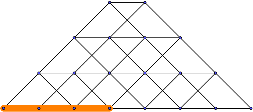
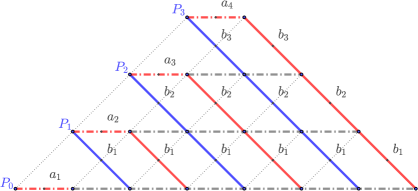
More generally, when computing mk=xkP0,P0subscript𝑚𝑘superscript𝑥𝑘subscript𝑃0subscript𝑃0m_{k}=\mathopen{}\mathclose{{}\left\langle x^{k}P_{0},P_{0}}\right\rangle, the recursive application of the recurrence relation (3.2) allows to decrease the power of x𝑥x from k𝑘k to 00 until each term in the development is proportional to the inner product of P0=1subscript𝑃01P_{0}=1 with another monic OP. The only nonzero such inner product is P0,P0=1subscript𝑃0subscript𝑃01\mathopen{}\mathclose{{}\left\langle P_{0},P_{0}}\right\rangle=1. Consequently, each nonzero term in the final development of mksubscript𝑚𝑘m_{k} corresponds to a path of length at most k𝑘k that leaves from the lower left corner of the graph in Figure 1(a) and ends up on the bottom row. In between, the path has to remain above the bottom row, and can only move North-East, East, or South-East. Each edge corresponds to picking one of the three terms in the recurrence relation (3.2). For example, the development of m3subscript𝑚3m_{3} in (4.7) corresponds to three such paths, shown in green in Figure 1(a). The product of the coefficients along each path forms the resulting term in the development.
Refer to caption
(a) The North-East, East, South-East edges associated to weights 111, ansubscript𝑎𝑛a_{n}, bnsubscript𝑏𝑛b_{n} are respectively represented as dashed, dash-dotted and solid lines. Note that on each dashed and dash-dotted line, the weight is constant.
Refer to caption
(b) 1a2b11subscript𝑎2subscript𝑏11\cdot a_{2}\cdot b_{1}
Refer to caption
(c) 1b2a11subscript𝑏2subscript𝑎11\cdot b_{2}\cdot a_{1}
Refer to caption
(d) a11b1subscript𝑎11subscript𝑏1a_{1}\cdot 1\cdot b_{1}
Refer to caption
(e) a1a1a1subscript𝑎1subscript𝑎1subscript𝑎1a_{1}\cdot a_{1}\cdot a_{1}
Figure 1: The lattice path of Hardy (2017) used to compute mn=xnP0,P0subscript𝑚𝑛superscript𝑥𝑛subscript𝑃0subscript𝑃0m_{n}=\mathopen{}\mathclose{{}\left\langle x^{n}P_{0},P_{0}}\right\rangle is displayed in 1(a). The paths used for the computation of m3subscript𝑚3m_{3} (4.7) are highlighted in 1(b)-1(e) with the corresponding weight as caption.

In the end, odd moments m2i1subscript𝑚2𝑖1m_{2i-1}, resp. even moments m2isubscript𝑚2𝑖m_{2i}, are the sum of the weights of the paths below the i𝑖i-th red, respectively blue path, counting from the bottom left. More precisely,

m2i1=aik=1i1bk+f1(a1:i1,b1:i2)andm2i=k=1ibk+f2(a1:i,b1:i1).formulae-sequencesubscript𝑚2𝑖1subscript𝑎𝑖superscriptsubscriptproduct𝑘1𝑖1subscript𝑏𝑘subscript𝑓1subscript𝑎:1𝑖1subscript𝑏:1𝑖2andsubscript𝑚2𝑖superscriptsubscriptproduct𝑘1𝑖subscript𝑏𝑘subscript𝑓2subscript𝑎:1𝑖subscript𝑏:1𝑖1m_{2i-1}={\color[rgb]{1,0,0}\definecolor[named]{pgfstrokecolor}{rgb}{1,0,0}a_{i}\prod_{k=1}^{i-1}b_{k}}+f_{1}(a_{1:i-1},b_{1:i-2})\quad\text{and}\quad m_{2i}={\color[rgb]{0,0,1}\definecolor[named]{pgfstrokecolor}{rgb}{0,0,1}\prod_{k=1}^{i}b_{k}}+f_{2}(a_{1:i},b_{1:i-1}). (4.8)

Thus, the Jacobian is the determinant of a triangular matrix

|m1:2N1a1:N,b1:N1|=|[m2i1ajm2i1bjm2iajm2ibj][m2i1aNm2iaN][m2N1ajm2N1bj]m2N1aN|i,j=1N1=i=1Nm2i1aii=1N1m2ibi\mathopen{}\mathclose{{}\left|\frac{\partial m_{1:2N-1}}{\partial a_{1:N},b_{1:N-1}}}\right|=\begin{vmatrix}\begin{bmatrix}\frac{\partial m_{2i-1}}{\partial a_{j}}&\frac{\partial m_{2i-1}}{\partial b_{j}}\\ \frac{\partial m_{2i}}{\partial a_{j}}&\frac{\partial m_{2i}}{\partial b_{j}}\end{bmatrix}&\begin{bmatrix}\frac{\partial m_{2i-1}}{\partial a_{N}}\\ \frac{\partial m_{2i}}{\partial a_{N}}\end{bmatrix}\\ \mathopen{}\mathclose{{}\left[\frac{\partial m_{2N-1}}{\partial a_{j}}\enspace\frac{\partial m_{2N-1}}{\partial b_{j}}}\right]&\frac{\partial m_{2N-1}}{\partial a_{N}}\\ \end{vmatrix}_{i,j=1}^{N-1}=\prod_{i=1}^{N}\frac{\partial m_{2i-1}}{\partial a_{i}}\prod_{i=1}^{N-1}\frac{\partial m_{2i}}{\partial b_{i}}\cdot

The formulation (4.8) yields

m2i1ai=k=1i1bkandm2ibi=k=1i1bk.formulae-sequencesubscript𝑚2𝑖1subscript𝑎𝑖superscriptsubscriptproduct𝑘1𝑖1subscript𝑏𝑘andsubscript𝑚2𝑖subscript𝑏𝑖superscriptsubscriptproduct𝑘1𝑖1subscript𝑏𝑘\frac{\partial m_{2i-1}}{\partial a_{i}}=\prod_{k=1}^{i-1}b_{k}\quad\text{and}\quad\frac{\partial m_{2i}}{\partial b_{i}}=\prod_{k=1}^{i-1}b_{k}.

Finally, we obtain

|m1:2N1a1:N,b1:N1|=i=1Nk=1i1bki=1N1k=1i1bk=[i=1Nk=1i1bk]2k=1N1bk=[n=1N1bnNn]2n=1N1bn,subscript𝑚:12𝑁1subscript𝑎:1𝑁subscript𝑏:1𝑁1superscriptsubscriptproduct𝑖1𝑁superscriptsubscriptproduct𝑘1𝑖1subscript𝑏𝑘superscriptsubscriptproduct𝑖1𝑁1superscriptsubscriptproduct𝑘1𝑖1subscript𝑏𝑘superscriptdelimited-[]superscriptsubscriptproduct𝑖1𝑁superscriptsubscriptproduct𝑘1𝑖1subscript𝑏𝑘2superscriptsubscriptproduct𝑘1𝑁1subscript𝑏𝑘limit-fromsuperscriptdelimited-[]superscriptsubscriptproduct𝑛1𝑁1superscriptsubscript𝑏𝑛𝑁𝑛2superscriptsubscriptproduct𝑛1𝑁1subscript𝑏𝑛,\displaystyle\mathopen{}\mathclose{{}\left|\frac{\partial m_{1:2N-1}}{\partial a_{1:N},b_{1:N-1}}}\right|=\prod_{i=1}^{N}\prod_{k=1}^{i-1}b_{k}\prod_{i=1}^{N-1}\prod_{k=1}^{i-1}b_{k}=\frac{\mathopen{}\mathclose{{}\left[\prod_{i=1}^{N}\prod_{k=1}^{i-1}b_{k}}\right]^{2}}{\prod_{k=1}^{N-1}b_{k}}=\frac{\mathopen{}\mathclose{{}\left[\prod_{n=1}^{N-1}b_{n}^{N-n}}\right]^{2}}{\prod_{n=1}^{N-1}b_{n}}\mathbin{\raisebox{2.15277pt}{,}}

which does not vanish since all bnsubscript𝑏𝑛b_{n}s are positive by construction. Finally, the last equality in (4.6) follows from Lemma 3.2. ∎

Propositions 4.1 and 4.2 now allow us to conclude that Favard’s map ψ=ρϕ𝜓𝜌italic-ϕ\psi=\rho\circ\phi (cf. Theorem 3.1) is a C1superscript𝐶1C^{1}-diffeomorphism, and compute its Jacobian.

Proposition 4.3.

Favard’s map ψ𝜓\psi is a C1superscript𝐶1C^{1}-diffeomorphism from \bbR>N×SNsuperscriptsubscript\bbR𝑁subscript𝑆𝑁\bbR_{>}^{N}\times S_{N} onto \bbRN×(0,+)N1superscript\bbR𝑁superscript0𝑁1\bbR^{N}\times(0,+\infty)^{N-1}, and

|x1:N,w1:N1a1:N,b1:N1|=n=1N1bn1n=1Nwn.subscript𝑥:1𝑁subscript𝑤:1𝑁1subscript𝑎:1𝑁subscript𝑏:1𝑁1superscriptsubscriptproduct𝑛1𝑁1superscriptsubscript𝑏𝑛1superscriptsubscriptproduct𝑛1𝑁subscript𝑤𝑛\mathopen{}\mathclose{{}\left|\frac{\partial x_{1:N},w_{1:N-1}}{\partial a_{1:N},b_{1:N-1}}}\right|=\prod_{n=1}^{N-1}b_{n}^{-1}\prod_{n=1}^{N}w_{n}. (4.9)

We now have all the ingredients to give an explicit proof of Theorem 2.4, of which the three classical tridiagonal models of Section 5 will be seen to be corollaries.

Proof of Theorem 2.4.

For simplicity we drop the indicator functions and rewrite the density of the nodes and weights as

(2.7)italic-(2.7italic-)\displaystyle\eqref{eq:joint_distribution_x_w} =(|Δ(x1,,xN)|2n=1Nwn)β2eTr[V(diag(x1,,xN))]n=1Nwn1dx1:Ndw1:N1absentsuperscriptsuperscriptΔsubscript𝑥1subscript𝑥𝑁2superscriptsubscriptproduct𝑛1𝑁subscript𝑤𝑛𝛽2superscripteTr𝑉diagsubscript𝑥1subscript𝑥𝑁superscriptsubscriptproduct𝑛1𝑁superscriptsubscript𝑤𝑛1dsubscript𝑥:1𝑁dsubscript𝑤:1𝑁1\displaystyle=\mathopen{}\mathclose{{}\left(\mathopen{}\mathclose{{}\left|\Delta\mathopen{}\mathclose{{}\left(x_{1},\dots,x_{N}}\right)}\right|^{2}\prod_{n=1}^{N}w_{n}}\right)^{\frac{\beta}{2}}\operatorname{\mathrm{e}}^{-\operatorname{Tr}\mathopen{}\mathclose{{}\left[V(\operatorname{diag}(x_{1},\dots,x_{N}))}\right]}\prod_{n=1}^{N}w_{n}^{-1}\mathrm{d}x_{1:N}\mathrm{d}w_{1:N-1}

Combining Lemma 3.2, and the fact that x1,,xNsubscript𝑥1subscript𝑥𝑁x_{1},\dots,x_{N} are the eigenvalues of J𝐚,𝐛subscript𝐽𝐚𝐛J_{\mathbf{a},\mathbf{b}}, the change of variables provided by Proposition 4.3 yields

(2.7)italic-(2.7italic-)\displaystyle\eqref{eq:joint_distribution_x_w} =(n=1N1bnNn)β2eTr[V(J𝐚,𝐛)]n=1Nwn1|x1:N,w1:N1a1:N,b1:N1|da1:Ndb1:N1absentsuperscriptsuperscriptsubscriptproduct𝑛1𝑁1superscriptsubscript𝑏𝑛𝑁𝑛𝛽2superscripteTr𝑉subscript𝐽𝐚𝐛superscriptsubscriptproduct𝑛1𝑁superscriptsubscript𝑤𝑛1subscript𝑥:1𝑁subscript𝑤:1𝑁1subscript𝑎:1𝑁subscript𝑏:1𝑁1dsubscript𝑎:1𝑁dsubscript𝑏:1𝑁1\displaystyle=\mathopen{}\mathclose{{}\left(\prod_{n=1}^{N-1}b_{n}^{N-n}}\right)^{\frac{\beta}{2}}\operatorname{\mathrm{e}}^{-\operatorname{Tr}\mathopen{}\mathclose{{}\left[V(J_{\mathbf{a},\mathbf{b}})}\right]}\prod_{n=1}^{N}w_{n}^{-1}\mathopen{}\mathclose{{}\left|\frac{\partial x_{1:N},w_{1:N-1}}{\partial a_{1:N},b_{1:N-1}}}\right|\mathrm{d}a_{1:N}\mathrm{d}b_{1:N-1}
=n=1N1bnβ2(Nn)1eTr[V(J𝐚,𝐛)]da1:Ndb1:N1,absentsuperscriptsubscriptproduct𝑛1𝑁1superscriptsubscript𝑏𝑛𝛽2𝑁𝑛1superscripteTr𝑉subscript𝐽𝐚𝐛dsubscript𝑎:1𝑁dsubscript𝑏:1𝑁1\displaystyle=\prod_{n=1}^{N-1}b_{n}^{\frac{\beta}{2}(N-n)-1}\operatorname{\mathrm{e}}^{-\operatorname{Tr}\mathopen{}\mathclose{{}\left[V(J_{\mathbf{a},\mathbf{b}})}\right]}\mathrm{d}a_{1:N}\mathrm{d}b_{1:N-1},

where the last equality follows from (4.9). ∎

5 Proving the three classical tridiagonal models

Theorem 2.4 gives the distribution over recurrence coefficients, from which one has to sample, in order for the atoms of the corresponding atomic measure to follow a given β𝛽\beta-ensemble. When the potential of the β𝛽\beta-ensemble is taken among three particular forms, the recurrence coefficients turn out to be independent with simple distributions. In particular, the recurrence coefficients are much simpler to sample than the complex joint distribution (1.1) of the atoms.

5.1 The Hβ𝛽\betaE and its tridiagonal model

The tridiagonal model associated to the Hermite β𝛽\beta-ensemble, cf. Theorem 2.1, follows from a direct application of Theorem 2.4 and the following immediate lemma.

Lemma 5.1.

Let J𝐚,𝐛subscript𝐽𝐚𝐛J_{\mathbf{a},\mathbf{b}} be a Jacobi matrix as defined by (2.1), with eigenvalues x1,,xNsubscript𝑥1subscript𝑥𝑁x_{1},\dots,x_{N}. It holds that

n=1Nxn=TrJ𝐚,𝐛=n=1Nanandn=1Nxn2=TrJ𝐚,𝐛2=n=1Nan2+2n=1N1bn.formulae-sequencesuperscriptsubscript𝑛1𝑁subscript𝑥𝑛Trsubscript𝐽𝐚𝐛superscriptsubscript𝑛1𝑁subscript𝑎𝑛andsuperscriptsubscript𝑛1𝑁superscriptsubscript𝑥𝑛2Trsuperscriptsubscript𝐽𝐚𝐛2superscriptsubscript𝑛1𝑁superscriptsubscript𝑎𝑛22superscriptsubscript𝑛1𝑁1subscript𝑏𝑛\sum_{n=1}^{N}x_{n}=\operatorname{Tr}J_{\mathbf{a},\mathbf{b}}=\sum_{n=1}^{N}a_{n}\quad\text{and}\quad\sum_{n=1}^{N}x_{n}^{2}=\operatorname{Tr}J_{\mathbf{a},\mathbf{b}}^{2}=\sum_{n=1}^{N}a_{n}^{2}+2\sum_{n=1}^{N-1}b_{n}. (5.1)
Proof of Theorem 2.1.

Starting from Theorem 2.4 it remains to express the term TrV(J𝐚,𝐛)Tr𝑉subscript𝐽𝐚𝐛\operatorname{Tr}V(J_{\mathbf{a},\mathbf{b}}), where V(x)=(xμ)22σ2=12σ2(x22μx+μ2)𝑉𝑥superscript𝑥𝜇22superscript𝜎212superscript𝜎2superscript𝑥22𝜇𝑥superscript𝜇2V(x)=\frac{(x-\mu)^{2}}{2\sigma^{2}}=\frac{1}{2\sigma^{2}}(x^{2}-2\mu x+\mu^{2}). To this end, Lemma 5.1 yields

TrV(J𝐚,𝐛)=12σ2[TrJ𝐚,𝐛22μTrJ𝐚,𝐛+Nμ2]=12σ2n=1N(anμ)2+1σ2n=1N1bn.Tr𝑉subscript𝐽𝐚𝐛12superscript𝜎2delimited-[]Trsuperscriptsubscript𝐽𝐚𝐛22𝜇Trsubscript𝐽𝐚𝐛𝑁superscript𝜇212superscript𝜎2superscriptsubscript𝑛1𝑁superscriptsubscript𝑎𝑛𝜇21superscript𝜎2superscriptsubscript𝑛1𝑁1subscript𝑏𝑛\operatorname{Tr}V(J_{\mathbf{a},\mathbf{b}})=\frac{1}{2\sigma^{2}}\mathopen{}\mathclose{{}\left[\operatorname{Tr}J_{\mathbf{a},\mathbf{b}}^{2}-2\mu\operatorname{Tr}J_{\mathbf{a},\mathbf{b}}+N\mu^{2}}\right]=\frac{1}{2\sigma^{2}}\sum_{n=1}^{N}(a_{n}-\mu)^{2}+\frac{1}{\sigma^{2}}\sum_{n=1}^{N-1}b_{n}.

Finally, we can plug this expression back into (2.7) to see that the entries of J𝐚,𝐛subscript𝐽𝐚𝐛J_{\mathbf{a},\mathbf{b}} are independently distributed, with joint distribution proportional to

n=1N1bnβ2(Nn)1e1σ2bndbnn=1Ne12σ2(anμ)2dan.superscriptsubscriptproduct𝑛1𝑁1superscriptsubscript𝑏𝑛𝛽2𝑁𝑛1superscripte1superscript𝜎2subscript𝑏𝑛dsubscript𝑏𝑛superscriptsubscriptproduct𝑛1𝑁superscripte12superscript𝜎2superscriptsubscript𝑎𝑛𝜇2dsubscript𝑎𝑛\prod_{n=1}^{N-1}b_{n}^{\frac{\beta}{2}(N-n)-1}\operatorname{\mathrm{e}}^{-\frac{1}{\sigma^{2}}b_{n}}\mathrm{d}b_{n}\prod_{n=1}^{N}\operatorname{\mathrm{e}}^{-\frac{1}{2\sigma^{2}}(a_{n}-\mu)^{2}}\mathrm{d}a_{n}. (5.2)

Note that when μ𝜇\mu is still supported on \mathbb{R}, but the potential is a more general polynomial, the recurrence parameters are no longer independent, but the interaction remains short range. This is what we later exploit in Section 6, where we derive a fast approximate sampler for various β𝛽\beta-ensembles with polynomial potentials.

5.2 The Lβ𝛽\betaE and its tridiagonal model

When the target β𝛽\beta-ensemble is supported on (0,+)0(0,+\infty), there is a natural reparametrization of the recurrence coefficients of μ𝜇\mu, which allows to express other quantities than those in Lemma 5.1. This leads to the tridiagonal model of Theorem 2.2 for the Laguerre β𝛽\beta-ensemble.

The reparametrization, denoted by ξ1,,ξ2N1>0subscript𝜉1subscript𝜉2𝑁10\xi_{1},\dots,\xi_{2N-1}>0, arose in the work of Stieltjes (1894) on continued fractions; see also Chihara (1978, 1971, Equation 9.12 in Corollary of Theorem 9.1; Equation 2) in the context of three-term recurrence relations. To introduce these new parameters, first note that since μ𝜇\mu is now supported on (0,+)0(0,+\infty), the recurrence relation (3.2) implies

an=Pn12xPn1,Pn1=Pn120xPn12(x)μ(dx)>0,n=1,,N.formulae-sequencesubscript𝑎𝑛superscriptnormsubscript𝑃𝑛12𝑥subscript𝑃𝑛1subscript𝑃𝑛1superscriptnormsubscript𝑃𝑛12superscriptsubscript0𝑥superscriptsubscript𝑃𝑛12𝑥𝜇d𝑥0𝑛1𝑁a_{n}=\mathopen{}\mathclose{{}\left\|P_{n-1}}\right\|^{-2}\mathopen{}\mathclose{{}\left\langle xP_{n-1},P_{n-1}}\right\rangle=\mathopen{}\mathclose{{}\left\|P_{n-1}}\right\|^{-2}\int_{0}^{\infty}xP_{n-1}^{2}(x)\mu(\mathrm{d}x)>0,\quad n=1,\dots,N. (5.3)

Now, we set

a1=ξ1,subscript𝑎1subscript𝜉1\displaystyle a_{1}=\xi_{1},{} an=ξ2n2+ξ2n1,for 2nN,formulae-sequencesubscript𝑎𝑛subscript𝜉2𝑛2subscript𝜉2𝑛1for 2𝑛𝑁\displaystyle a_{n}=\xi_{2n-2}+\xi_{2n-1},\quad\text{for }2\leq n\leq N, (5.4)
   and bn=ξ2n1ξ2n,for 1nN1.formulae-sequencesubscript𝑏𝑛subscript𝜉2𝑛1subscript𝜉2𝑛for 1𝑛𝑁1\displaystyle b_{n}=\xi_{2n-1}\xi_{2n},\quad\text{for }1\leq n\leq N-1.

Equivalently, the new parameters correspond to the Cholesky factorization

J𝐚,𝐛=ΞΞ𝖳,whereΞ=(ξ1(0)ξ2ξ3(0)ξ2N2ξ2N1).formulae-sequencesubscript𝐽𝐚𝐛ΞsuperscriptΞ𝖳whereΞmatrixsubscript𝜉1missing-subexpressionmissing-subexpression0subscript𝜉2subscript𝜉3missing-subexpressionmissing-subexpressionmissing-subexpressionmissing-subexpression0missing-subexpressionsubscript𝜉2𝑁2subscript𝜉2𝑁1J_{\mathbf{a},\mathbf{b}}=\Xi~{}\Xi^{\mathsf{\scriptscriptstyle T}},\quad\text{where}\quad\Xi=\begin{pmatrix}\sqrt{\xi_{1}}&&&(0)\\ \sqrt{\xi_{2}}&\sqrt{\xi_{3}}&&\\ &\ddots&\ddots&\\ (0)&&\sqrt{\xi_{2N-2}}&\sqrt{\xi_{2N-1}}\end{pmatrix}. (5.5)

Note that this bidiagonal transformation is reminiscent of the construction of the tridiagonal model for the Lβ𝛽\betaE, where Dumitriu & Edelman (2002) bidiagonalize a random Gaussian matrix. The following proposition shows that the change of variables replacing the recurrence coefficients by ξ1:2N1subscript𝜉:12𝑁1\xi_{1:2N-1} is valid.

Proposition 5.1.

Consider μ𝜇\mu supported on (0,+)0(0,+\infty), then the corresponding Jacobi matrix (2.1) factorizes uniquely as J𝐚,𝐛=ΞΞ𝖳subscript𝐽𝐚𝐛ΞsuperscriptΞ𝖳J_{\mathbf{a},\mathbf{b}}=\Xi~{}\Xi^{\mathsf{\scriptscriptstyle T}}, where ΞΞ\Xi is given by (5.5). Moreover, the mapping

(ξ1,,ξ2N1)(a1:N,b1:N1),subscript𝜉1subscript𝜉2𝑁1subscript𝑎:1𝑁subscript𝑏:1𝑁1\begin{array}[]{rcl}(\xi_{1},\dots,\xi_{2N-1})&\longmapsto&(a_{1:N},b_{1:N-1}),\end{array} (5.6)

defined by (5.4) is a C1superscript𝐶1C^{1}-diffeomorphism of (0,+)2N1superscript02𝑁1(0,+\infty)^{2N-1} onto itself, and its Jacobian reads

|a1:N,b1:N1ξ1:2N1|=i=1N1ξ2i1.subscript𝑎:1𝑁subscript𝑏:1𝑁1subscript𝜉:12𝑁1superscriptsubscriptproduct𝑖1𝑁1subscript𝜉2𝑖1\mathopen{}\mathclose{{}\left|\frac{\partial a_{1:N},b_{1:N-1}}{\partial\xi_{1:2N-1}}}\right|=\prod_{i=1}^{N-1}\xi_{2i-1}. (5.7)
Proof.

Given that J𝐚,𝐛subscript𝐽𝐚𝐛J_{\mathbf{a},\mathbf{b}} is symmetric with positive eigenvalues, the Cholesky factorization J𝐚,𝐛=ΞΞ𝖳subscript𝐽𝐚𝐛ΞsuperscriptΞ𝖳J_{\mathbf{a},\mathbf{b}}=\Xi~{}\Xi^{\mathsf{\scriptscriptstyle T}} is unique, see, e.g., Golub & Van Loan (2013, Theorem 4.2.7). Moreover, since J𝐚,𝐛subscript𝐽𝐚𝐛J_{\mathbf{a},\mathbf{b}} is tridiagonal, the factor ΞΞ\Xi can only be bidiagonal. Hence, the mapping (5.6) is injective (and even bijective) and C1superscript𝐶1C^{1} because it is polynomial. Finally, by definition of the transformation (5.4), the Jacobian reads as the determinant of a triangular matrix

|a1:N,b1:N1ξ1:2N1|=|[aiξ2j1aiξ2jbiξ2j1biξ2j]i,j=1N1[aiξ2N1biξ2N1]i=1N1[aNξ2j1aNξ2j]j=1N1aNξ2N1|=i=1Naiξ2i1=1i=1N1biξ2i=ξ2i1\mathopen{}\mathclose{{}\left|\frac{\partial a_{1:N},b_{1:N-1}}{\partial\xi_{1:2N-1}}}\right|=\begin{vmatrix}\begin{bmatrix}\frac{\partial a_{i}}{\partial\xi_{2j-1}}&\frac{\partial a_{i}}{\partial\xi_{2j}}\\ \frac{\partial b_{i}}{\partial\xi_{2j-1}}&\frac{\partial b_{i}}{\partial\xi_{2j}}\end{bmatrix}_{i,j=1}^{N-1}&\begin{bmatrix}\frac{\partial a_{i}}{\partial\xi_{2N-1}}\\ \frac{\partial b_{i}}{\partial\xi_{2N-1}}\end{bmatrix}_{i=1}^{N-1}\\ \begin{bmatrix}\frac{\partial a_{N}}{\partial\xi_{2j-1}}\enspace\frac{\partial a_{N}}{\partial\xi_{2j}}\end{bmatrix}_{j=1}^{N-1}&\frac{\partial a_{N}}{\partial\xi_{2N-1}}\\ \end{vmatrix}=\prod_{i=1}^{N}\underbrace{\frac{\partial a_{i}}{\partial\xi_{2i-1}}}_{=1}\prod_{i=1}^{N-1}\underbrace{\frac{\partial b_{i}}{\partial\xi_{2i}}}_{=\xi_{2i-1}}\cdot

For our purpose, the Cholesky factorization (5.5) is ideal to express the key quantities that appear in the Lβ𝛽\betaE. The proof of the corresponding tridiagonal model, cf. Theorem 2.2, follows from a direct application of Theorem 2.4 and the following immediate lemma.

Lemma 5.2.

Let J𝐚,𝐛=ΞΞ𝖳subscript𝐽𝐚𝐛ΞsuperscriptΞ𝖳J_{\mathbf{a},\mathbf{b}}=\Xi~{}\Xi^{\mathsf{\scriptscriptstyle T}} as in (5.5) and note x1,,xNsubscript𝑥1subscript𝑥𝑁x_{1},\dots,x_{N} its eigenvalues. Then,

n=1Nxn=TrJ𝐚,𝐛=n=12N1ξnandn=1Nxn=detJ𝐚,𝐛=n=1Nξ2n1.formulae-sequencesuperscriptsubscript𝑛1𝑁subscript𝑥𝑛Trsubscript𝐽𝐚𝐛superscriptsubscript𝑛12𝑁1subscript𝜉𝑛andsuperscriptsubscriptproduct𝑛1𝑁subscript𝑥𝑛subscript𝐽𝐚𝐛superscriptsubscriptproduct𝑛1𝑁subscript𝜉2𝑛1\sum_{n=1}^{N}x_{n}=\operatorname{Tr}J_{\mathbf{a},\mathbf{b}}=\sum_{n=1}^{2N-1}\xi_{n}\quad\text{and}\quad\prod_{n=1}^{N}x_{n}=\det J_{\mathbf{a},\mathbf{b}}=\prod_{n=1}^{N}\xi_{2n-1}. (5.8)
Proof of Theorem 2.2.

Applying Lemma 5.2 to the V(x)=(k1)log(x)+xθ𝑉𝑥𝑘1𝑥𝑥𝜃V(x)=-(k-1)\log(x)+\frac{x}{\theta} yields

exp[TrV(J𝐚,𝐛)]Tr𝑉subscript𝐽𝐚𝐛\displaystyle\exp\mathopen{}\mathclose{{}\left[-\operatorname{Tr}V(J_{\mathbf{a},\mathbf{b}})}\right] =(detJ𝐚,𝐛)k1exp(1θTrJ𝐚,𝐛)absentsuperscriptsubscript𝐽𝐚𝐛𝑘11𝜃Trsubscript𝐽𝐚𝐛\displaystyle=\mathopen{}\mathclose{{}\left(\det J_{\mathbf{a},\mathbf{b}}}\right)^{k-1}\exp\mathopen{}\mathclose{{}\left(-\frac{1}{\theta}\operatorname{Tr}J_{\mathbf{a},\mathbf{b}}}\right)
=(5.8)n=1Nξ2n1k1exp(1θn=12N1ξn).superscriptsubscriptabsentitalic-(5.8italic-)superscriptsubscriptproduct𝑛1𝑁superscriptsubscript𝜉2𝑛1𝑘11𝜃superscriptsubscript𝑛12𝑁1subscript𝜉𝑛\displaystyle\operatornamewithlimits{=}\limits_{\begin{subarray}{c}\end{subarray}}^{\begin{subarray}{c}\eqref{eq:sum-prod_x_xi}\end{subarray}}\prod_{n=1}^{N}\xi_{2n-1}^{k-1}\exp\mathopen{}\mathclose{{}\left(-\frac{1}{\theta}\sum_{n=1}^{2N-1}\xi_{n}}\right). (5.9)

Starting from (2.8), Proposition 5.1 gives the joint distribution of the underlying ξ1:2N1subscript𝜉:12𝑁1\xi_{1:2N-1} parameters as proportional to

n=1N1bnβ2(Nn)1eTrV(J𝐚,𝐛)da1:Ndb1:N1superscriptsubscriptproduct𝑛1𝑁1superscriptsubscript𝑏𝑛𝛽2𝑁𝑛1superscripteTr𝑉subscript𝐽𝐚𝐛dsubscript𝑎:1𝑁dsubscript𝑏:1𝑁1\displaystyle\prod_{n=1}^{N-1}b_{n}^{\frac{\beta}{2}(N-n)-1}\operatorname{\mathrm{e}}^{-\operatorname{Tr}V(J_{\mathbf{a},\mathbf{b}})}\mathrm{d}a_{1:N}\mathrm{d}b_{1:N-1}
=(5.4)n=1N1(ξ2n1ξ2n)β2(Nn)1eTrV(J𝐚,𝐛)|a1:N,b1:N1ξ1:2N1|dξ1:2N1italic-(5.4italic-)superscriptsubscriptproduct𝑛1𝑁1superscriptsubscript𝜉2𝑛1subscript𝜉2𝑛𝛽2𝑁𝑛1superscripteTr𝑉subscript𝐽𝐚𝐛subscript𝑎:1𝑁subscript𝑏:1𝑁1subscript𝜉:12𝑁1dsubscript𝜉:12𝑁1\displaystyle\overset{\eqref{eq:def_ab_xi}}{=}\prod_{n=1}^{N-1}\mathopen{}\mathclose{{}\left(\xi_{2n-1}\xi_{2n}}\right)^{\frac{\beta}{2}(N-n)-1}\operatorname{\mathrm{e}}^{-\operatorname{Tr}V(J_{\mathbf{a},\mathbf{b}})}\mathopen{}\mathclose{{}\left|\frac{\partial a_{1:N},b_{1:N-1}}{\partial\xi_{1:2N-1}}}\right|\mathrm{d}\xi_{1:2N-1}
=(5.7)n=1N1ξ2n1β2(Nn)1ξ2nβ2(Nn)1eTrV(J𝐚,𝐛)n=1N1ξ2n1dξ1:2N1italic-(5.7italic-)superscriptsubscriptproduct𝑛1𝑁1superscriptsubscript𝜉2𝑛1𝛽2𝑁𝑛cancel1superscriptsubscript𝜉2𝑛𝛽2𝑁𝑛1superscripteTr𝑉subscript𝐽𝐚𝐛cancelsuperscriptsubscriptproduct𝑛1𝑁1subscript𝜉2𝑛1dsubscript𝜉:12𝑁1\displaystyle\overset{\eqref{eq:jacobian_xi_a,b}}{=}\prod_{n=1}^{N-1}\xi_{2n-1}^{\frac{\beta}{2}(N-n)-\cancel{1}}\xi_{2n}^{\frac{\beta}{2}(N-n)-1}\operatorname{\mathrm{e}}^{-\operatorname{Tr}V(J_{\mathbf{a},\mathbf{b}})}\cancel{\prod_{n=1}^{N-1}\xi_{2n-1}}\mathrm{d}\xi_{1:2N-1} (5.10)
=(5.9)n=1Nξ2n1β2(Nn)n=1N1ξ2nβ2(Nn)1(n=1Nξ2n1)k1e1θn=12N1ξndξ1:2N1italic-(5.9italic-)superscriptsubscriptproduct𝑛1𝑁superscriptsubscript𝜉2𝑛1𝛽2𝑁𝑛superscriptsubscriptproduct𝑛1𝑁1superscriptsubscript𝜉2𝑛𝛽2𝑁𝑛1superscriptsuperscriptsubscriptproduct𝑛1𝑁subscript𝜉2𝑛1𝑘1superscripte1𝜃superscriptsubscript𝑛12𝑁1subscript𝜉𝑛dsubscript𝜉:12𝑁1\displaystyle\overset{\eqref{eq:exp_-_Tr_V_Jab_xi}}{=}\prod_{n=1}^{N}\xi_{2n-1}^{\frac{\beta}{2}(N-n)}\prod_{n=1}^{N-1}\xi_{2n}^{\frac{\beta}{2}(N-n)-1}\Big{(}\prod_{n=1}^{N}\xi_{2n-1}\Big{)}^{k-1}\operatorname{\mathrm{e}}^{-\frac{1}{\theta}\sum_{n=1}^{2N-1}\xi_{n}}\mathrm{d}\xi_{1:2N-1}

In the next section, we introduce another reparametrization of the recurrence coefficients, this time when μ𝜇\mu is supported in a compact interval: the canonical moments of Dette & Studden (1997).

5.3 The Jβ𝛽\betaE and its tridiagonal model

Finding a tridiagonal model for the Jβ𝛽\betaE was left as an open problem by Dumitriu & Edelman (2002, IV B). The latter was addressed by Killip & Nenciu (2004, Theorem 2) in their study of the quindiagonal model associated to the circular ensemble. However, the authors acknowledged that lifting the points on the unit circle to apply their result represents a winding detour to prove the Jβ𝛽\betaE. Besides, the Jacobian required by this method was obtained by indirect means by Killip & Nenciu (2007, Lemma 4.3). Subsequently, Forrester & Rains (2006, Theorem 2) obtained the Jacobian more directly.

We can actually prove the tridiagonal model of Theorem 2.3 by reparametrizing the Jacobi matrix J𝐚,𝐛subscript𝐽𝐚𝐛J_{\mathbf{a},\mathbf{b}} again, this time using canonical moments (Dette & Studden, 1997, Chapter 1). In essence, the result can be found in the work of Gamboa & Rouault (2010) and Dette & Nagel (2012), but we rephrase it as just another consequence of Theorem 2.4.

Before formally introducing them, let us mention that canonical moments and their complex counterpart were successfully used to investigate the connection between randomized moments problems, orthogonal polynomials, and optimal design (Dette & Studden, 1997) and in random matrix theory (Gamboa & Rouault, 2010; Gamboa et al., 2016). In particular, canonical moments can be thought of as a reparametrization of the moments, where 0<cn<10subscript𝑐𝑛10<c_{n}<1 represents the relative position of the n𝑛n-th moment mnsubscript𝑚𝑛m_{n} in the range of all possible moments associated to measure with compatible previous moments m1,,mn1subscript𝑚1subscript𝑚𝑛1m_{1},\dots,m_{n-1}, see Dette & Studden (1997).

Throughout this section, we assume that the N𝑁N-atomic measure μ𝜇\mu is supported on (0,1)01(0,1). In particular, with (ξn)subscript𝜉𝑛(\xi_{n}) the parameters introduced in Section 5.2, it comes

0<ξ2n2+ξ2n1=an=Pn12xPn1,Pn1<1,n=2,,N.formulae-sequence0subscript𝜉2𝑛2subscript𝜉2𝑛1subscript𝑎𝑛superscriptnormsubscript𝑃𝑛12𝑥subscript𝑃𝑛1subscript𝑃𝑛11𝑛2𝑁0<\xi_{2n-2}+\xi_{2n-1}=a_{n}=\mathopen{}\mathclose{{}\left\|P_{n-1}}\right\|^{-2}\mathopen{}\mathclose{{}\left\langle xP_{n-1},P_{n-1}}\right\rangle<1,\quad n=2,\dots,N.

Similarly, ξ1=a1(0,1).subscript𝜉1subscript𝑎101\xi_{1}=a_{1}\in(0,1). This implies 0<ξn<10subscript𝜉𝑛10<\xi_{n}<1 for all 1n2N11𝑛2𝑁11\leq n\leq 2N-1. Following the work of Wall (1940) on chain sequences and continued fractions, we introduce a new parametrization of the recurrence coefficients.

Lemma 5.3 (Wall).

Assume μ𝜇\mu is supported on (0,1)01(0,1), there exist a sequence (cn)(0,1)subscript𝑐𝑛superscript01(c_{n})\in(0,1)^{\mathbb{N}} such that

ξ1=c1andξn=(1cn1)cn,2n2N1.formulae-sequencesubscript𝜉1subscript𝑐1andformulae-sequencesubscript𝜉𝑛1subscript𝑐𝑛1subscript𝑐𝑛for-all2𝑛2𝑁1\xi_{1}=c_{1}\quad\text{and}\quad\xi_{n}=(1-c_{n-1})c_{n},\quad\forall 2\leq n\leq 2N-1. (5.11)

We do not prove Lemma 5.3 and refer to Wall (1940, Theorem 6.1); see also Chihara (1978, Chapter 3) for more details on chain sequences. We simply note that defining (cn)subscript𝑐𝑛(c_{n}) in (5.11) is straightforward, the nontrivial part of the lemma is that 0<cn<10subscript𝑐𝑛10<c_{n}<1 for all n𝑛n. We also note that the cnsubscript𝑐𝑛c_{n}s are today known as the canonical moments of μ𝜇\mu; see the monograph of Dette & Studden (1997).

The following proposition shows that the change of variables replacing ξ𝜉\xi by c𝑐c is valid.

Proposition 5.2.

Consider μ𝜇\mu supported on (0,1)01(0,1), then the corresponding Jacobi matrix (2.1) can be parametrized in terms of the canonical moments following (5.4) and (5.11). Moreover, the mapping

(c1,,c2N1)(ξ1,,ξ2N1),subscript𝑐1subscript𝑐2𝑁1subscript𝜉1subscript𝜉2𝑁1\begin{array}[]{rcl}(c_{1},\dots,c_{2N-1})&\longmapsto&(\xi_{1},\dots,\xi_{2N-1}),\end{array} (5.12)

defined by (5.11) is a C1superscript𝐶1C^{1}-diffeomorphism of (0,1)2N1superscript012𝑁1(0,1)^{2N-1} onto itself, and its Jacobian reads

|ξ1:2N1c1:2N1|=n=12N2(1cn).subscript𝜉:12𝑁1subscript𝑐:12𝑁1superscriptsubscriptproduct𝑛12𝑁21subscript𝑐𝑛\mathopen{}\mathclose{{}\left|\frac{\partial\xi_{1:2N-1}}{\partial c_{1:2N-1}}}\right|=\prod_{n=1}^{2N-2}(1-c_{n}). (5.13)
Proof.

The map (5.12) is a bijection by definition and Lemma 5.3, and C1superscript𝐶1C^{1} because it is polynomial. Then, by definition of the transformation (5.11), the Jacobian is the determinant of a triangular matrix

|ξ1:2N1c1:2N1|=n=12N1ξncn=1n=22N1(1cn1)=n=12N2(1cn).subscript𝜉:12𝑁1subscript𝑐:12𝑁1superscriptsubscriptproduct𝑛12𝑁1subscript𝜉𝑛subscript𝑐𝑛1superscriptsubscriptproduct𝑛22𝑁11subscript𝑐𝑛1superscriptsubscriptproduct𝑛12𝑁21subscript𝑐𝑛\mathopen{}\mathclose{{}\left|\frac{\partial\xi_{1:2N-1}}{\partial c_{1:2N-1}}}\right|=\prod_{n=1}^{2N-1}\frac{\partial\xi_{n}}{\partial c_{n}}=1\cdot\prod_{n=2}^{2N-1}(1-c_{n-1})=\prod_{n=1}^{2N-2}(1-c_{n}).

For our purpose, the canonical moment parametrization is ideal to express the key quantities that appear in the Jβ𝛽\betaE. The proof of the corresponding tridiagonal model in Theorem 2.3 is again a direct application of Proposition 5.2 and the following lemma.

Lemma 5.4.

It holds that

n=1Nxn=detJ𝐚,𝐛=n=1Nc2n1n=1N1(1c2n)andn=1N(1xn)=det[INJ]=n=12N1(1cn).formulae-sequencesuperscriptsubscriptproduct𝑛1𝑁subscript𝑥𝑛subscript𝐽𝐚𝐛superscriptsubscriptproduct𝑛1𝑁subscript𝑐2𝑛1superscriptsubscriptproduct𝑛1𝑁11subscript𝑐2𝑛andsuperscriptsubscriptproduct𝑛1𝑁1subscript𝑥𝑛delimited-[]subscript𝐼𝑁𝐽superscriptsubscriptproduct𝑛12𝑁11subscript𝑐𝑛\prod_{n=1}^{N}x_{n}=\det J_{\mathbf{a},\mathbf{b}}=\prod_{n=1}^{N}c_{2n-1}\prod_{n=1}^{N-1}(1-c_{2n})\quad\text{and}\quad\prod_{n=1}^{N}(1-x_{n})=\det[I_{N}-J]=\prod_{n=1}^{2N-1}(1-c_{n}). (5.14)
Proof.

First, combine the result of Lemma 5.2 and the definition of the canonical moments in (5.11) to get

n=1Nxn=ξ1n=2Nξ2n1=c1n=2N(1c2n2)c2n1=n=1Nc2n1(1c2n).superscriptsubscriptproduct𝑛1𝑁subscript𝑥𝑛subscript𝜉1superscriptsubscriptproduct𝑛2𝑁subscript𝜉2𝑛1subscript𝑐1superscriptsubscriptproduct𝑛2𝑁1subscript𝑐2𝑛2subscript𝑐2𝑛1superscriptsubscriptproduct𝑛1𝑁subscript𝑐2𝑛11subscript𝑐2𝑛\prod_{n=1}^{N}x_{n}=\xi_{1}\prod_{n=2}^{N}\xi_{2n-1}=c_{1}\prod_{n=2}^{N}(1-c_{2n-2})c_{2n-1}=\prod_{n=1}^{N}c_{2n-1}(1-c_{2n}). (5.15)

Then, Lemma 3.1 yields

n=1N(1xn)=|H¯2N1||H¯2N2|\prod_{n=1}^{N}(1-x_{n})=\frac{\mathopen{}\mathclose{{}\left|\overline{H}_{2N-1}}\right|}{\mathopen{}\mathclose{{}\left|\underline{H}_{2N-2}}\right|}\cdot (5.16)

The denominator can be expressed in terms of the ξ1:2N1subscript𝜉:12𝑁1\xi_{1:2N-1} parameters

|H¯2N2|2=(3.17)n=1N1bnNn=(5.4)n=1N1[ξ2n1ξ2n]Nn.superscriptsubscript¯𝐻2𝑁22superscriptsubscriptabsentitalic-(3.17italic-)superscriptsubscriptproduct𝑛1𝑁1superscriptsubscript𝑏𝑛𝑁𝑛superscriptsubscriptabsentitalic-(5.4italic-)superscriptsubscriptproduct𝑛1𝑁1superscriptdelimited-[]subscript𝜉2𝑛1subscript𝜉2𝑛𝑁𝑛\mathopen{}\mathclose{{}\left|\underline{H}_{2N-2}}\right|^{2}\operatornamewithlimits{=}\limits_{\begin{subarray}{c}\end{subarray}}^{\begin{subarray}{c}\eqref{eq:H_2N-2_Vandermonde_prod_b}\end{subarray}}\prod_{n=1}^{N-1}b_{n}^{N-n}\operatornamewithlimits{=}\limits_{\begin{subarray}{c}\end{subarray}}^{\begin{subarray}{c}\eqref{eq:def_ab_xi}\end{subarray}}\prod_{n=1}^{N-1}\mathopen{}\mathclose{{}\left[\xi_{2n-1}\xi_{2n}}\right]^{N-n}. (5.17)

For the numerator, we follow Dette & Studden (1997, Theorem 1.4.10) who introduced additional quantities γ1:2N1subscript𝛾:12𝑁1\gamma_{1:2N-1} to get

|H¯2N1|=γ1Nn=1N1[γ2nγ2n+1]Nn,subscript¯𝐻2𝑁1superscriptsubscript𝛾1𝑁superscriptsubscriptproduct𝑛1𝑁1superscriptdelimited-[]subscript𝛾2𝑛subscript𝛾2𝑛1𝑁𝑛\mathopen{}\mathclose{{}\left|\overline{H}_{2N-1}}\right|=\gamma_{1}^{N}\prod_{n=1}^{N-1}\mathopen{}\mathclose{{}\left[\gamma_{2n}\gamma_{2n+1}}\right]^{N-n}, (5.18)

where

{ξ1=c1γ1=1c1and{ξn=(1cn1)cnγn=cn1(1cn)2n2N1.casessubscript𝜉1subscript𝑐1otherwisesubscript𝛾11subscript𝑐1otherwiseandcasessubscript𝜉𝑛1subscript𝑐𝑛1subscript𝑐𝑛otherwisesubscript𝛾𝑛subscript𝑐𝑛11subscript𝑐𝑛otherwisefor-all2𝑛2𝑁1\begin{cases}\xi_{1}=c_{1}\\ \gamma_{1}=1-c_{1}\end{cases}\quad\text{and}\quad\begin{cases}\xi_{n}=(1-c_{n-1})c_{n}\\ \gamma_{n}=c_{n-1}(1-c_{n})\end{cases}\forall 2\leq n\leq 2N-1. (5.19)

We plug these results back into (5.16), and conclude that

n=1N(1xn)superscriptsubscriptproduct𝑛1𝑁1subscript𝑥𝑛\displaystyle\prod_{n=1}^{N}(1-x_{n}) =|H¯2N1||H¯2N2|=γ1Nn=1N1[γ2nγ2n+1ξ2n1ξ2n]Nnabsentsubscript¯𝐻2𝑁1subscript¯𝐻2𝑁2superscriptsubscript𝛾1𝑁superscriptsubscriptproduct𝑛1𝑁1superscriptdelimited-[]subscript𝛾2𝑛subscript𝛾2𝑛1subscript𝜉2𝑛1subscript𝜉2𝑛𝑁𝑛\displaystyle=\frac{\mathopen{}\mathclose{{}\left|\overline{H}_{2N-1}}\right|}{\mathopen{}\mathclose{{}\left|\underline{H}_{2N-2}}\right|}=\gamma_{1}^{N}\prod_{n=1}^{N-1}\mathopen{}\mathclose{{}\left[\frac{\gamma_{2n}\gamma_{2n+1}}{\xi_{2n-1}\xi_{2n}}}\right]^{N-n}
=(1c1)N[c1(1c2)c2(1c3)c1(1c1)c2]N1n=2N1[c2n1(1c2n)c2n(1c2n+1)(1c2n2)c2n1(1c2n1)c2n]Nnabsentsuperscript1subscript𝑐1𝑁superscriptdelimited-[]cancelsubscript𝑐11subscript𝑐2cancelsubscript𝑐21subscript𝑐3cancelsubscript𝑐11subscript𝑐1cancelsubscript𝑐2𝑁1superscriptsubscriptproduct𝑛2𝑁1superscriptdelimited-[]cancelsubscript𝑐2𝑛11subscript𝑐2𝑛cancelsubscript𝑐2𝑛1subscript𝑐2𝑛11subscript𝑐2𝑛2cancelsubscript𝑐2𝑛11subscript𝑐2𝑛1cancelsubscript𝑐2𝑛𝑁𝑛\displaystyle=(1-c_{1})^{N}\mathopen{}\mathclose{{}\left[\frac{\cancel{c_{1}}(1-c_{2})\cancel{c_{2}}(1-c_{3})}{\cancel{c_{1}}(1-c_{1})\cancel{c_{2}}}}\right]^{N-1}\prod_{n=2}^{N-1}\mathopen{}\mathclose{{}\left[\frac{\cancel{c_{2n-1}}(1-c_{2n})\cancel{c_{2n}}(1-c_{2n+1})}{(1-c_{2n-2})\cancel{c_{2n-1}}(1-c_{2n-1})\cancel{c_{2n}}}}\right]^{N-n}
=(1c1)Nn=1N1[1c2n+11c2n1]Nn(1c2)N1n=2N1[1c2n1c2n2]Nnabsentsuperscript1subscript𝑐1𝑁superscriptsubscriptproduct𝑛1𝑁1superscriptdelimited-[]1subscript𝑐2𝑛11subscript𝑐2𝑛1𝑁𝑛superscript1subscript𝑐2𝑁1superscriptsubscriptproduct𝑛2𝑁1superscriptdelimited-[]1subscript𝑐2𝑛1subscript𝑐2𝑛2𝑁𝑛\displaystyle=(1-c_{1})^{N}\prod_{n=1}^{N-1}\mathopen{}\mathclose{{}\left[\frac{1-c_{2n+1}}{1-c_{2n-1}}}\right]^{N-n}~{}(1-c_{2})^{N-1}\prod_{n=2}^{N-1}\mathopen{}\mathclose{{}\left[\frac{1-c_{2n}}{1-c_{2n-2}}}\right]^{N-n}
=n=1N(1c2n1)n=1N1(1c2n).absentsuperscriptsubscriptproduct𝑛1𝑁1subscript𝑐2𝑛1superscriptsubscriptproduct𝑛1𝑁11subscript𝑐2𝑛\displaystyle=\prod_{n=1}^{N}\mathopen{}\mathclose{{}\left(1-c_{2n-1}}\right)\prod_{n=1}^{N-1}\mathopen{}\mathclose{{}\left(1-c_{2n}}\right).

Proof of Theorem 2.3.

Considering the potential V(x)=[(a1)log(x)+(b1)log(1x)]𝑉𝑥delimited-[]𝑎1𝑥𝑏11𝑥V(x)=-[(a-1)\log(x)+(b-1)\log(1-x)], Lemma 5.4 yields

exp[TrV(J𝐚,𝐛)]Tr𝑉subscript𝐽𝐚𝐛\displaystyle\exp[-\operatorname{Tr}V(J_{\mathbf{a},\mathbf{b}})] =[detJ]a1[detINJ]b1absentsuperscriptdelimited-[]𝐽𝑎1superscriptdelimited-[]subscript𝐼𝑁𝐽𝑏1\displaystyle=\mathopen{}\mathclose{{}\left[\det J}\right]^{a-1}\mathopen{}\mathclose{{}\left[\det{I_{N}-J}}\right]^{b-1}
=(5.14)n=1Nc2n1a1(1c2n1)b1n=1N1(1c2n)a+b2.superscriptsubscriptabsentitalic-(5.14italic-)product𝑛1𝑁superscriptsubscript𝑐2𝑛1𝑎1superscript1subscript𝑐2𝑛1𝑏1product𝑛1𝑁1superscript1subscript𝑐2𝑛𝑎𝑏2\displaystyle\operatornamewithlimits{=}\limits_{\begin{subarray}{c}\end{subarray}}^{\begin{subarray}{c}\eqref{eq:prod_x,1-x_c}\end{subarray}}\prod{n=1}{N}c_{2n-1}^{a-1}(1-c_{2n-1})^{b-1}\prod{n=1}{N-1}(1-c_{2n})^{a+b-2}. (5.20)

Starting from (5.10), Proposition 5.2 allows us to express the joint distribution of the canonical moments as

n=1N1[ξ2n1ξ2n]β2(Nn)ξ2neTrV(J𝐚,𝐛)|ξ1:2N1c1:2N1|dc1:2N1superscriptsubscriptproduct𝑛1𝑁1superscriptdelimited-[]subscript𝜉2𝑛1subscript𝜉2𝑛𝛽2𝑁𝑛subscript𝜉2𝑛superscripteTr𝑉subscript𝐽𝐚𝐛subscript𝜉:12𝑁1subscript𝑐:12𝑁1dsubscript𝑐:12𝑁1\displaystyle\prod_{n=1}^{N-1}\frac{\mathopen{}\mathclose{{}\left[\xi_{2n-1}\xi_{2n}}\right]^{\frac{\beta}{2}(N-n)}}{\xi_{2n}}\operatorname{\mathrm{e}}^{-\operatorname{Tr}V(J_{\mathbf{a},\mathbf{b}})}\mathopen{}\mathclose{{}\left|\frac{\partial\xi_{1:2N-1}}{\partial c_{1:2N-1}}}\right|\mathrm{d}c_{1:2N-1}
=(5.13)n=1N1[ξ2n1ξ2n]β2(Nn)ξ2nn=12N2(1cn)eTrV(J𝐚,𝐛)dc1:2N1superscriptsubscriptabsentitalic-(5.13italic-)superscriptsubscriptproduct𝑛1𝑁1superscriptdelimited-[]subscript𝜉2𝑛1subscript𝜉2𝑛𝛽2𝑁𝑛subscript𝜉2𝑛superscriptsubscriptproduct𝑛12𝑁21subscript𝑐𝑛superscripteTr𝑉subscript𝐽𝐚𝐛dsubscript𝑐:12𝑁1\displaystyle\operatornamewithlimits{=}\limits_{\begin{subarray}{c}\end{subarray}}^{\begin{subarray}{c}\eqref{eq:jacobian_c_xi}\end{subarray}}\prod_{n=1}^{N-1}\frac{\mathopen{}\mathclose{{}\left[\xi_{2n-1}\xi_{2n}}\right]^{\frac{\beta}{2}(N-n)}}{\xi_{2n}}\prod_{n=1}^{2N-2}(1-c_{n})\operatorname{\mathrm{e}}^{-\operatorname{Tr}V(J_{\mathbf{a},\mathbf{b}})}\mathrm{d}c_{1:2N-1}
=(5.11)[c1(1c1)c2]β2(N1)(1c1)c2n=2N1[(1c2n2)c2n1(1c2n1)c2n]β2(Nn)(1c2n1)c2nsuperscriptsubscriptabsentitalic-(5.11italic-)superscriptdelimited-[]subscript𝑐11subscript𝑐1subscript𝑐2𝛽2𝑁1cancel1subscript𝑐1subscript𝑐2superscriptsubscriptproduct𝑛2𝑁1superscriptdelimited-[]1subscript𝑐2𝑛2subscript𝑐2𝑛11subscript𝑐2𝑛1subscript𝑐2𝑛𝛽2𝑁𝑛cancel1subscript𝑐2𝑛1subscript𝑐2𝑛\displaystyle\operatornamewithlimits{=}\limits_{\begin{subarray}{c}\end{subarray}}^{\begin{subarray}{c}\eqref{eq:def_xi_c}\end{subarray}}\frac{\mathopen{}\mathclose{{}\left[c_{1}(1-c_{1})c_{2}}\right]^{\frac{\beta}{2}(N-1)}}{\cancel{(1-c_{1})}c_{2}}\prod_{n=2}^{N-1}\frac{\mathopen{}\mathclose{{}\left[(1-c_{2n-2})c_{2n-1}(1-c_{2n-1})c_{2n}}\right]^{\frac{\beta}{2}(N-n)}}{\cancel{(1-c_{2n-1})}c_{2n}}
n=1N1(1c2n1)(1c2n)eTrV(J𝐚,𝐛)dc1:2N1superscriptsubscriptproduct𝑛1𝑁1cancel1subscript𝑐2𝑛11subscript𝑐2𝑛superscripteTr𝑉subscript𝐽𝐚𝐛dsubscript𝑐:12𝑁1\displaystyle\qquad\qquad\prod_{n=1}^{N-1}\cancel{(1-c_{2n-1})}(1-c_{2n})\operatorname{\mathrm{e}}^{-\operatorname{Tr}V(J_{\mathbf{a},\mathbf{b}})}\mathrm{d}c_{1:2N-1}
=n=1N[c2n1(1c2n1)]β2(Nn)n=1N1c2nβ2(Nn)1(1c2n)β2(Nn1)+1eTrV(J𝐚,𝐛)dc1:2N1absentsuperscriptsubscriptproduct𝑛1𝑁superscriptdelimited-[]subscript𝑐2𝑛11subscript𝑐2𝑛1𝛽2𝑁𝑛superscriptsubscriptproduct𝑛1𝑁1superscriptsubscript𝑐2𝑛𝛽2𝑁𝑛1superscript1subscript𝑐2𝑛𝛽2𝑁𝑛11superscripteTr𝑉subscript𝐽𝐚𝐛dsubscript𝑐:12𝑁1\displaystyle=\prod_{n=1}^{N}\mathopen{}\mathclose{{}\left[c_{2n-1}(1-c_{2n-1})}\right]^{\frac{\beta}{2}(N-n)}\prod_{n=1}^{N-1}c_{2n}^{\frac{\beta}{2}(N-n)-1}(1-c_{2n})^{\frac{\beta}{2}(N-n-1)+1}\operatorname{\mathrm{e}}^{-\operatorname{Tr}V(J_{\mathbf{a},\mathbf{b}})}\mathrm{d}c_{1:2N-1}
=(5.20)n=1Nc2n1β2(Nn)+a1(1c2n1)β2(Nn)+b1n=1N1c2nβ2(Nn)1(1c2n)β2(Nn1)+a+b1dc1:2N1.italic-(5.20italic-)product𝑛1𝑁superscriptsubscript𝑐2𝑛1𝛽2𝑁𝑛𝑎1superscript1subscript𝑐2𝑛1𝛽2𝑁𝑛𝑏1product𝑛1𝑁1superscriptsubscript𝑐2𝑛𝛽2𝑁𝑛1superscript1subscript𝑐2𝑛𝛽2𝑁𝑛1𝑎𝑏1dsubscript𝑐:12𝑁1\displaystyle\overset{\eqref{eq:exp_-_Tr_V_Jab_c}}{=}\prod{n=1}{N}c_{2n-1}^{\frac{\beta}{2}(N-n)+a-1}(1-c_{2n-1})^{\frac{\beta}{2}(N-n)+b-1}\prod{n=1}{N-1}c_{2n}^{\frac{\beta}{2}(N-n)-1}(1-c_{2n})^{\frac{\beta}{2}(N-n-1)+a+b-1}\mathrm{d}c_{1:2N-1}.

6 Gibbs sampling tridiagonal models associated to polynomial potentials

As seen in Section 5, for the specific potentials associated to the Hermite, Laguerre, and Jacobi β𝛽\beta-ensembles, the successive parametrizations of the corresponding Jacobi matrix J𝐚,𝐛subscript𝐽𝐚𝐛J_{\mathbf{a},\mathbf{b}} yield independent coefficients with easy-to-sample distributions. Thus, computing the eigenvalues of the corresponding randomized tridiagonal Jacobi matrices gives \calO(N2)\calOsuperscript𝑁2\calO(N^{2}) exact samplers. However, when the potential V𝑉V is generic, these Jacobi parameters may not be independent anymore. For polynomial potentials, this dependence remains mild, in the sense that each parameter remains independent from the rest conditionally on a few “neighboring” parameters. As we shall see in this section, simple Gibbs samplers in the space of these Jacobi parameters can provide surprisingly fast-mixing approximate samplers for β𝛽\beta-ensembles. In short, we study a Gibbs sampler on tridiagonal matrices, which we can diagonalize in \calO(N2)\calOsuperscript𝑁2\calO(N^{2}) to obtain approximate samples from a given β𝛽\beta-ensemble. This approach is in contrast with that of Li & Menon (2013) and Chafaï & Ferré (2018), who used MCMC directly on the original space where the particles {x1,,xN}subscript𝑥1subscript𝑥𝑁\mathopen{}\mathclose{{}\left\{x_{1},\dots,x_{N}}\right\} live.

Our starting point is Proposition 2 of Krishnapur et al. (2016), which we rederived as Theorem 2.4. In short, a Jacobi matrix J𝐚,𝐛subscript𝐽𝐚𝐛J_{\mathbf{a},\mathbf{b}} with coefficients distributed as

(a1,b1,,aN1,bN1,aN)i=1N1biβ2(Ni)1expTrV(Ja,b)da1:N,b1:N1,similar-tosubscript𝑎1subscript𝑏1subscript𝑎𝑁1subscript𝑏𝑁1subscript𝑎𝑁superscriptsubscriptproduct𝑖1𝑁1superscriptsubscript𝑏𝑖𝛽2𝑁𝑖1superscriptTr𝑉subscript𝐽𝑎𝑏dsubscript𝑎:1𝑁subscript𝑏:1𝑁1(a_{1},b_{1},\dots,a_{N-1},b_{N-1},a_{N})\sim\prod_{i=1}^{N-1}b_{i}^{\frac{\beta}{2}(N-i)-1}\exp^{-\operatorname{Tr}V(J_{a,b})}\mathrm{d}a_{1:N},b_{1:N-1}, (6.1)

has eigenvalues distributed according to the β𝛽\beta-ensemble (1.1) with potential V𝑉V. Krishnapur et al. (2016) already mention their intuition that a Gibbs chain with invariant measure (6.1) and a polynomial potential would mix fast, in \calO(logN)\calO𝑁\calO(\log N), due to the short range interaction between the coefficients. From an algorithmic point of view, the explicit conditionals in (6.1) similarly invite to use a Gibbs sampler, which we investigate in this section. For the sake of presentation, we fix the potential to be a polynomial with even degree at most 6 and positive leading coefficient, i.e.

V(x)=g6x6+g5x5+g4x4+g3x3+g2x2+g1x.𝑉𝑥subscript𝑔6superscript𝑥6cancelsubscript𝑔5superscript𝑥5subscript𝑔4superscript𝑥4subscript𝑔3superscript𝑥3subscript𝑔2superscript𝑥2subscript𝑔1𝑥V(x)=g_{6}x^{6}+\cancel{g_{5}x^{5}}+g_{4}x^{4}+g_{3}x^{3}+g_{2}x^{2}+g_{1}x. (6.2)

The absence of a term of degree 555 in (6.2) comes from practical reasons detailed in Section 6.1. While the method applies more generally, we restrict ourselves to potentials of the form (6.2) because (i)𝑖(i) it already goes beyond the numerical state-of-the-art, (ii)𝑖𝑖(ii) it is rich enough to require different sampling schemes for different conditionals depending on the coefficients in (6.2), and (iii)𝑖𝑖𝑖(iii) the theory of sextic potentials is advanced enough that we have means to empirically assess the convergence of our samplers.

The associated implementation is available in our DPPy toolbox. We also provide a companion Python notebook where we illustrate our sampler on various potentials, see https://github.com/guilgautier/DPPy/tree/master/notebooks.

6.1 Sampling from the conditionals

We implement a systematic scan Gibbs sampler (Robert & Casella, 2004, Chapter 10) to approximately sample from the distribution (6.1) on the Jacobi coefficients. Writing the conditionals in closed form for the generic sextic potential (6.2) is cumbersome, but we do it for a specific instance in Example 6.1 below. The expansion of TrV(J𝐚,𝐛)Tr𝑉subscript𝐽𝐚𝐛\operatorname{Tr}V(J_{\mathbf{a},\mathbf{b}}) in (6.1) reveals that the size of the Markov blanket of each coefficient grows with degVdeg𝑉\operatorname{deg}V. Quoting Krishnapur et al. (2016, Section 1), variables with indices that are degV/2deg𝑉2\operatorname{deg}V/2 apart are conditionally independent given the variables in between. In other words, the Jacobi coefficients a1,,aN,b1,,bN1subscript𝑎1subscript𝑎𝑁subscript𝑏1subscript𝑏𝑁1a_{1},\dots,a_{N},b_{1},\dots,b_{N-1} have a more short-range interaction than the corresponding particles x1,,xNsubscript𝑥1subscript𝑥𝑁x_{1},\dots,x_{N}. Gibbs sampling can leverage that property.

For 1iN1𝑖𝑁1\leq i\leq N, let \bfai=(a1,,ai1,ai+1,,aN)subscript\bfa𝑖subscript𝑎1subscript𝑎𝑖1subscript𝑎𝑖1subscript𝑎𝑁\bfa_{\setminus i}=(a_{1},\dots,a_{i-1},a_{i+1},\dots,a_{N}). Similarly, for 1jN11𝑗𝑁11\leq j\leq N-1, let \bfbj=(b1,,bj1,bj+1,,bN1)subscript\bfb𝑗subscript𝑏1subscript𝑏𝑗1subscript𝑏𝑗1subscript𝑏𝑁1\bfb_{\setminus j}=(b_{1},\dots,b_{j-1},b_{j+1},\dots,b_{N-1}). In practice, we define one complete Gibbs pass as sampling from an\bfan,\bfbconditionalsubscript𝑎𝑛subscript\bfa𝑛\bfba_{n}\mid\bfa_{\setminus n},\bfb, and then bn\bfa,\bfbnconditionalsubscript𝑏𝑛\bfasubscript\bfb𝑛b_{n}\mid\bfa,\bfb_{\setminus n}, for each n𝑛n in turn. We avoid the term of degree 555 in (6.2) to make sure that the conditionals bn\bfa,\bfbnconditionalsubscript𝑏𝑛\bfasubscript\bfb𝑛b_{n}\mid\bfa,\bfb_{\setminus n} are always log-concave, while the conditionals an\bfan,\bfbconditionalsubscript𝑎𝑛subscript\bfa𝑛\bfba_{n}\mid\bfa_{\setminus n},\bfb are log-concave if g2>0subscript𝑔20g_{2}>0 and g3=g6=0subscript𝑔3subscript𝑔60g_{3}=g_{6}=0. Univariate log-concave densities are interesting from a sampling point of view, since they are usually amenable to efficient rejection sampling.

In our case, for every log-concave conditional, the mode of the corresponding density can be derived analytically. We can thus use the tailored rejection sampler of Devroye (2012), with an expected 555 rejection steps per draw; see Example 6.1 for details. The overall algorithm is given in Algorithm 1.

When the conditionals an\bfan,\bfbconditionalsubscript𝑎𝑛subscript\bfa𝑛\bfba_{n}\mid\bfa_{\setminus n},\bfb are not log-concave, we switch from a Gibbs algorithm to a Metropolis-within-Gibbs algorithm, and replace exact sampling of the corresponding conditional by a draw from a Metropolis-Hastings kernel. More specifically, since the log of the conditional densities an\bfan,\bfbconditionalsubscript𝑎𝑛subscript\bfa𝑛\bfba_{n}\mid\bfa_{\setminus n},\bfb are polynomials, they are easy to differentiate, and we use their gradient in a Metropolis-adjusted Langevin kernel (MALA, see, e.g., Robert & Casella, 2004, Section 7.8.5).

Algorithm 1 Gibbs sampler to sample from (6.1) with β>0𝛽0\beta>0 and V𝑉V as in (6.2)
  Input: inverse temperature β𝛽\beta, potential V𝑉V, number of MCMC steps T𝑇T
  Initialize a1==aN=b1= =bN1=0subscript𝑎1subscript𝑎𝑁subscript𝑏1 subscript𝑏𝑁10a_{1}=\cdots=a_{N}=b_{1}= \cdots=b_{N-1}=0
  for t=1𝑡1t=1 to T𝑇T do
     for n=1𝑛1n=1 to N𝑁N do
        Sample an\bfan,\bfbconditionalsubscript𝑎𝑛subscript\bfa𝑛\bfba_{n}\mid\bfa_{\setminus n},\bfb
        if n<N𝑛𝑁n<N then
           Sample bn\bfa,\bfbnconditionalsubscript𝑏𝑛\bfasubscript\bfb𝑛b_{n}\mid\bfa,\bfb_{\setminus n}
        end if
     end for
     x1t,,xNt=eigvals(J𝐚,𝐛)superscriptsubscript𝑥1𝑡superscriptsubscript𝑥𝑁𝑡eigvalssubscript𝐽𝐚𝐛x_{1}^{t},\dots,x_{N}^{t}=\operatorname{eigvals}(J_{\mathbf{a},\mathbf{b}})
  end for

Example 6.1 (Quartic potential).

Let V(x)=g4x4+g2x2𝑉𝑥subscript𝑔4superscript𝑥4subscript𝑔2superscript𝑥2V(x)=g_{4}x^{4}+g_{2}x^{2}. With the convention a0=aN+1=b0=bN=0subscript𝑎0subscript𝑎𝑁1subscript𝑏0subscript𝑏𝑁0a_{0}=a_{N+1}=b_{0}=b_{N}=0, the conditionals write as follows.
For all n{1,,N}𝑛1𝑁n\in\{1,\dots,N\},

an\bfan,\bfbexp[[g4an4+an2[g2+4g4(bn1+bn)]+4g4an(an1bn1+an+1bn)]],missing-subexpressionconditionalsubscript𝑎𝑛subscript\bfa𝑛\bfbmissing-subexpressionsimilar-toabsentdelimited-[]subscript𝑔4superscriptsubscript𝑎𝑛4superscriptsubscript𝑎𝑛2delimited-[]subscript𝑔24subscript𝑔4subscript𝑏𝑛1subscript𝑏𝑛4subscript𝑔4subscript𝑎𝑛subscript𝑎𝑛1subscript𝑏𝑛1subscript𝑎𝑛1subscript𝑏𝑛\displaystyle\begin{aligned} &a_{n}\mid\bfa_{\setminus n},\bfb\\ &\sim\exp\mathopen{}\mathclose{{}\left[-\mathopen{}\mathclose{{}\left[g_{4}a_{n}^{4}+a_{n}^{2}\mathopen{}\mathclose{{}\left[g_{2}+4g_{4}(b_{n-1}+b_{n})}\right]+4g_{4}a_{n}(a_{n-1}b_{n-1}+a_{n+1}b_{n})}\right]}\right],\end{aligned} (6.3)

For all n{1,,N1}𝑛1𝑁1n\in\{1,\dots,N-1\},

bn\bfa,\bfbnbnβ2(Ni)1exp[2[g4bn2+bn[g2+2g4(an2+anan+1+an+12+bn1+bn+1)]]].missing-subexpressionconditionalsubscript𝑏𝑛\bfasubscript\bfb𝑛missing-subexpressionsimilar-toabsentsuperscriptsubscript𝑏𝑛𝛽2𝑁𝑖12delimited-[]subscript𝑔4superscriptsubscript𝑏𝑛2subscript𝑏𝑛delimited-[]subscript𝑔22subscript𝑔4superscriptsubscript𝑎𝑛2subscript𝑎𝑛subscript𝑎𝑛1superscriptsubscript𝑎𝑛12subscript𝑏𝑛1subscript𝑏𝑛1\displaystyle\begin{aligned} &b_{n}\mid\bfa,\bfb_{\setminus n}\\ &\sim b_{n}^{\frac{\beta}{2}(N-i)-1}\exp\mathopen{}\mathclose{{}\left[-2\mathopen{}\mathclose{{}\left[g_{4}b_{n}^{2}+b_{n}\mathopen{}\mathclose{{}\left[g_{2}+2g_{4}(a_{n}^{2}+a_{n}a_{n+1}+a_{n+1}^{2}+b_{n-1}+b_{n+1})}\right]}\right]}\right].\end{aligned} (6.4)

In this case, for g2,g4>0subscript𝑔2subscript𝑔40g_{2},g_{4}>0, the conditionals given in Equations 6.3 and 6.4 are unnormalized and log\log-concave, with easy-to-find modes. Thus, the rejection sampling technique of Devroye (2012) applies, with an expected number of rejections equal to 555. Given an unnormalized and log\log-concave target density π𝜋\pi with mode m=argmaxyπ(y)𝑚subscriptargmax𝑦𝜋𝑦m=\operatornamewithlimits{argmax}_{y}\pi(y), Devroye (2012) constructs a piecewise dominating function hh comprising 3 plateaus and 2 exponential tails such that h/π5𝜋5\int h/\int\pi\leq 5. The breakpoints m+2u,m+u,m+v,m+2v𝑚2𝑢𝑚𝑢𝑚𝑣𝑚2𝑣m+2u,m+u,m+v,m+2v are located on both sides of the mode, where u<0<v𝑢0𝑣u<0<v satisfy π(m+x)π(m)/4π(m+2x)𝜋𝑚𝑥𝜋𝑚4𝜋𝑚2𝑥\pi(m+x)\geq\pi(m)/4\geq\pi(m+2x). Such u𝑢u and v𝑣v can be found using a simple bisection method. In practice, we compute u<0<vsuperscript𝑢0superscript𝑣u^{\prime}<0<v^{\prime} solutions of π(m+x)=π(m)/4𝜋𝑚𝑥𝜋𝑚4\pi(m+x)=\pi(m)/4 and assign u=u/2𝑢superscript𝑢2u=u^{\prime}/2 and v=v/2𝑣superscript𝑣2v=v^{\prime}/2, see Figure 2.

Refer to caption
(a) An example conditional (6.3)
Refer to caption
(b) An example conditional (6.4)
Figure 2: Construction of the dominating function hh (solid line) of Devroye (2012) to perform rejection sampling with a log-concave target π𝜋\pi (dashed line), the mode of which needs to be analytically tractable.

6.2 Example simulations and empirical study of the convergence

In this section, we investigate the convergence of the Gibbs sampler detailed in Section 6.1. We sample from β𝛽\beta-ensembles with potential W(x)=βN2V(x)𝑊𝑥𝛽𝑁2𝑉𝑥W(x)=\frac{\beta N}{2}V(x), for various choices of V𝑉V of the form (6.2). The rescaling in W𝑊W is applied to capture the weak convergence of the empirical distribution of the particles towards the corresponding equilibrium measure μeqsubscript𝜇eq\mu_{\text{eq}}; see e.g., Deift (2000, Section 6.1). Intuitively, the rescaling balances the effect of the Vandermonde determinant and that of the potential V𝑉V in (1.1).

6.2.1 Convergence of the marginals

Let (xnt)1nNsubscriptsuperscriptsubscript𝑥𝑛𝑡1𝑛𝑁(x_{n}^{t})_{1\leq n\leq N} be the vector of ordered particles after t𝑡t full Gibbs passes, that is, after t𝑡t outer iterations of Algorithm 1. A first quantity to monitor is how well the empirical distribution μ^Nt=N1n=1Nδxntsuperscriptsubscript^𝜇𝑁𝑡superscript𝑁1superscriptsubscript𝑛1𝑁subscript𝛿superscriptsubscript𝑥𝑛𝑡\widehat{\mu}_{N}^{t}=N^{-1}\sum_{n=1}^{N}\delta_{x_{n}^{t}} approximates, as t𝑡t grows, the empirical distribution of the target β𝛽\beta-ensemble

μ^N=1Nn=1Nδxn,where {x1,,xN} is drawn from (1.1).subscript^𝜇𝑁1𝑁superscriptsubscript𝑛1𝑁subscript𝛿subscript𝑥𝑛where subscript𝑥1subscript𝑥𝑁 is drawn from (1.1).\widehat{\mu}_{N}=\frac{1}{N}\sum\limits_{n=1}^{N}\delta_{x_{n}},\quad\text{where }\{x_{1},\dots,x_{N}\}\text{ is drawn from \eqref{eq:joint_distribution_beta_ensemble}.}

It turns out that, under assumptions on the potential V𝑉V that are satisfied by (6.2), the random measure μ^Nsubscript^𝜇𝑁\widehat{\mu}_{N} is itself well approximated when N1much-greater-than𝑁1N\gg 1 by a (deterministic) measure μeqsubscript𝜇eq\mathrm{\mu_{eq}} called the equilibrium measure of the potential. This statement can be made rigorous; see for instance the large deviation principle with fast rate 1/N21superscript𝑁21/N^{2} in (Serfaty, 2015, Theorem 2.3).

Two observations are in order. First, the fast rate hints that the approximation should hold even for moderate values of N𝑁N, as we shall confirm later on in our simulations. Second, μeqsubscript𝜇eq\mathrm{\mu_{eq}} is known analytically for a few choices of polynomial potentials. Thus, for these potentials, we compare draws from μ^Nt=N1n=1Nδxntsuperscriptsubscript^𝜇𝑁𝑡superscript𝑁1superscriptsubscript𝑛1𝑁subscript𝛿superscriptsubscript𝑥𝑛𝑡\widehat{\mu}_{N}^{t}=N^{-1}\sum_{n=1}^{N}\delta_{x_{n}^{t}} with μeqsubscript𝜇eq\mu_{\text{eq}}, to assess convergence of our marginals μ^Ntsubscriptsuperscript^𝜇𝑡𝑁\widehat{\mu}^{t}_{N} as t𝑡t grows. This is in line with the experiments of Li & Menon (2013), Olver et al. (2014) and Chafaï & Ferré (2018).

The quartic potential.

The equilibrium measure μeqsubscript𝜇eq\mu_{\text{eq}} is available in closed form for potentials proportional to x2dsuperscript𝑥2𝑑x^{2d} (Deift, 2000, Proposition 6.156). We consider again V(x)=14x4𝑉𝑥14superscript𝑥4V(x)=\frac{1}{4}x^{4}, as in Example 6.1. In this case all conditionals are log-concave, and can thus be sampled exactly, cf. Section 6.1. Figure 3 shows the agregation of the marginal histograms of 100010001000 independent runs, after each of the first few Gibbs passes.

Observe that convergence to the equilibrium measure is extremely fast: beyond t=3𝑡3t=3 Gibbs passes, the histograms are visually indistinguishable from the equilibrium measure. This observation is quantitatively monitored in Figure 3, where we plot the logarithm of the Lsubscript𝐿L_{\infty} distance between the empirical cdf of μ^Ntsuperscriptsubscript^𝜇𝑁𝑡\widehat{\mu}_{N}^{t} and the cdf of μeqsubscript𝜇eq\mathrm{\mu_{eq}}.

Refer to caption
(a) N=10𝑁10N=10
Refer to caption
(b) N=20𝑁20N=20
Refer to caption
(c) N=50𝑁50N=50
Refer to caption
(d) N=100𝑁100N=100
Refer to caption
(e) N=150𝑁150N=150
Refer to caption
(f) N=150𝑁150N=150
Figure 3: For β=2𝛽2\beta=2 and V(x)=14x4𝑉𝑥14superscript𝑥4V(x)=\frac{1}{4}x^{4}, panels 3(a)-3(e) give a visual display of the convergence of the empirical marginal distribution μNtsuperscriptsubscript𝜇𝑁𝑡\mu_{N}^{t} of the eigenvalues constructed from 100010001000 independent chains. Each colored line corresponds to a Gibbs pass t{1,2,3,}𝑡123t\in\{1,2,3,...\}, while the equilibrium pdf is shown as a black line on each panel. Different panels correspond to increasing values of N𝑁N. Panel 3(f) shows the supremum norm of the difference between the cdf of μeqsubscript𝜇eq\mathrm{\mu_{eq}} and the cdf of μ^Ntsuperscriptsubscript^𝜇𝑁𝑡\widehat{\mu}_{N}^{t} as a function of the number t𝑡t of Gibbs passes.
Other potentials of degree 444.

We also consider the potential V(x)=120x4415x3+15x2+85x𝑉𝑥120superscript𝑥4415superscript𝑥315superscript𝑥285𝑥V(x)=\frac{1}{20}x^{4}-\frac{4}{15}x^{3}+\frac{1}{5}x^{2}+\frac{8}{5}x and potentials of the form V(x)=g2x2+14x4𝑉𝑥subscript𝑔2superscript𝑥214superscript𝑥4V(x)=g_{2}x^{2}+\frac{1}{4}x^{4} where we vary g2subscript𝑔2g_{2}. Except the case where g20subscript𝑔20g_{2}\geq 0, the conditionals an\bfan,\bfbconditionalsubscript𝑎𝑛subscript\bfa𝑛\bfba_{n}\mid\bfa_{\setminus n},\bfb are not log concave and we sample from them using a few steps of MALA. This allows us to select various qualitative behaviors of μeqsubscript𝜇eq\mathrm{\mu_{eq}}, which may become dissymmetric (Claeys et al., 2009; Olver et al., 2014, Example 1.2; Section 3.2), or supported by more than one connected component (Molinari, 2018, Figure 4). Our approach allows to simulate from the corresponding β𝛽\beta-ensembles in regimes yet unexplored. Figure 4 shows good agreement of marginal histograms of a single sample of N=1000𝑁1000N=1000 points with the equilibrium distribution after only t=10𝑡10t=10 Gibbs passes.

Refer to caption
(a) V(x)=14x4+12x2𝑉𝑥14superscript𝑥412superscript𝑥2V(x)=\frac{1}{4}x^{4}+\frac{1}{2}x^{2}
Refer to caption
(b) V(x)=14x4x2𝑉𝑥14superscript𝑥4superscript𝑥2V(x)=\frac{1}{4}x^{4}-x^{2}
Refer to caption
(c) V(x)=14x454x2𝑉𝑥14superscript𝑥454superscript𝑥2V(x)=\frac{1}{4}x^{4}-\frac{5}{4}x^{2}
Refer to caption
(d) V(x)=120x4415x3+15x2+85x𝑉𝑥120superscript𝑥4415superscript𝑥315superscript𝑥285𝑥V(x)=\frac{1}{20}x^{4}-\frac{4}{15}x^{3}+\frac{1}{5}x^{2}+\frac{8}{5}x
Figure 4: For various choices of potentials V𝑉V of degree 444 and β=2𝛽2\beta=2, each panel shows the histogram of a sample from μNtsuperscriptsubscript𝜇𝑁𝑡\mu_{N}^{t}, with N=1000𝑁1000N=1000 points after t=10𝑡10t=10 Gibbs passes. The corresponding equilibrium measures are superimposed in black.
The sextic potential.

We extend the derivations of Example 6.1 and consider sampling from the β𝛽\beta-ensemble with potential V(x)=16x6𝑉𝑥16superscript𝑥6V(x)=\frac{1}{6}x^{6}. The corresponding equilibrium distribution can be derived from Deift (2000, Proposition 6.156). In this case, the conditionals an\bfan,\bfbconditionalsubscript𝑎𝑛subscript\bfa𝑛\bfba_{n}\mid\bfa_{\setminus n},\bfb are not log-concave and we cannot use the exact rejection sampler of Devroye (2012). Instead, we switch to a Metropolis-within-Gibbs sampler and make a few steps of MALA; see Section 6.1.

One free parameter is the number of MALA steps in one Gibbs pass. We empirically observed (not shown) that this number has an influence on the number of Gibbs passes needed to reach the plateau in Figure 5(d). Manually setting the number of MALA steps per Gibbs pass to 100 was enough for rapid overall convergence in our experiments, and larger values did not significantly influence the fit in Figure 5, which is already striking after less than 10 Gibbs passes.
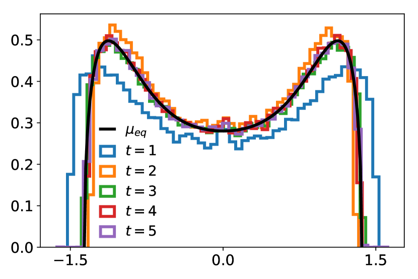
Refer to caption
(a) N=50𝑁50N=50
Refer to caption
(b) N=100𝑁100N=100
Refer to caption
(c) N=200𝑁200N=200
Refer to caption
(d) Convergence of the empirical cdf
Figure 5: For β=2𝛽2\beta=2 and V(x)=16x6𝑉𝑥16superscript𝑥6V(x)=\frac{1}{6}x^{6}, panels 5(a)-5(c) give a visual display of the convergence of the empirical marginal distribution μNtsuperscriptsubscript𝜇𝑁𝑡\mu_{N}^{t} of the eigenvalues constructed from 100010001000 independent chains. Each colored line corresponds to a Gibbs pass t{1,2,3,}𝑡123t\in\{1,2,3,...\}, while the equilibrium pdf is shown as a black line on each panel. Different panels correspond to increasing values of N𝑁N. Panel 5(d) shows the supremum norm of the difference between the cdf of μeqsubscript𝜇eq\mathrm{\mu_{eq}} and the cdf of μ^Ntsuperscriptsubscript^𝜇𝑁𝑡\widehat{\mu}_{N}^{t} as a function of the number t𝑡t of Gibbs passes.

6.2.2 Fluctuations of the largest eigenvalue

After looking at the global behavior of the eigenvalues, we zoom at the right edge of the support of μ𝜇\mu to study the local behavior of our approximate samples. We do this for the quartic and sextic potentials. When β=2𝛽2\beta=2, the target β𝛽\beta-ensemble is determinantal and we can test the adequation of the largest atom of μ^Ntsuperscriptsubscript^𝜇𝑁𝑡\widehat{\mu}_{N}^{t} to the universal Tracy-Widom limiting distribution (Deift & Gioev, 2005, Corollary 1.3). We implemented the cumulative distribution function (cdf) of the Tracy-Widom law following the work of Bornemann (2009), and rescale the eigenvalues as Olver & Trogdon (2014, Section 3.2).

For each potential, we run 100010001000 independent chains and record only the largest eigenvalue of each chain after each Gibbs pass. Figure 6 and Figure 7 show the histograms of the rescaled largest particles after a few Gibbs passes, respectively for the quartic and sextic potential. More quantitatively, in Figure 8 we monitor the convergence to the Tracy-Widom distribution across Gibbs passes, by computing the supremum distance between the empirical cdf of the largest eigenvalue and the cdf of the Tracy-Widom law.

For the quartic potential, we observe that the adequation with the cdf of the Tracy-Widom law gets tighter as N𝑁N grows, and again only a few passes of the Gibbs sampler are sufficient to reach a plateau.

In contrast, for the sextic ensemble there seems to be an impassable gap, as if the rescaling was not adequate or the Tracy-Widom law was not the proper limiting distribution. This is despite the square root singularity at the right edge of the equilibrium distribution (Deift, 2000, Section 6.1). In particular, a simple Kolmogorov-Smirnov test at level 0.050.050.05 would reject the adequation to Tracy-Widom. Part of this effect might be due to the fact that the conditionals are not sampled exactly in the sextic case, though.
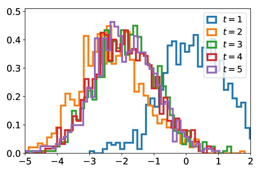
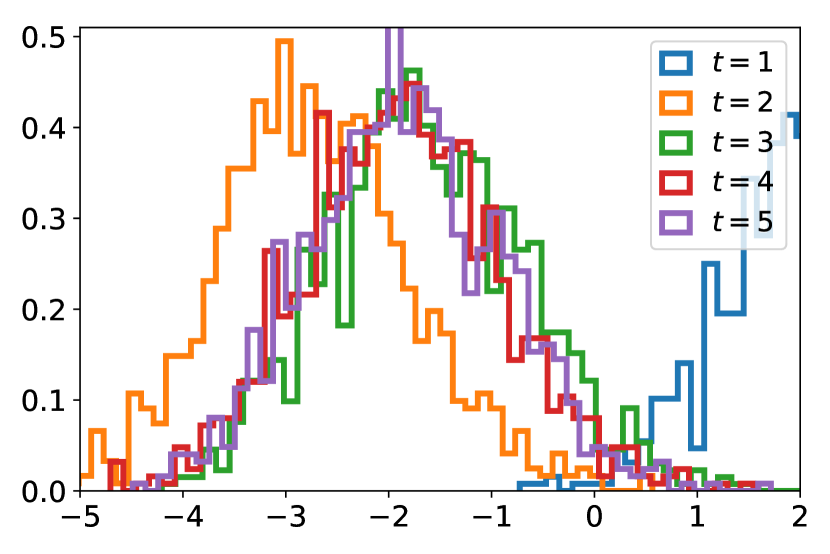
Refer to caption
(a) N=20𝑁20N=20
Refer to caption
(b) N=50𝑁50N=50
Refer to caption
(c) N=100𝑁100N=100
Refer to caption
(d) N=250𝑁250N=250
Figure 6: For β=2𝛽2\beta=2 and V(x)=14x4𝑉𝑥14superscript𝑥4V(x)=\frac{1}{4}x^{4}, we give a visual display of the convergence of the empirical distribution of the largest atom of μNtsuperscriptsubscript𝜇𝑁𝑡\mu_{N}^{t} constructed from 100010001000 independent chains to the Tracy-Widom distribution. Each colored line corresponds to a Gibbs pass t{1,2,3,}𝑡123t\in\{1,2,3,...\}. Different panels correspond to increasing values of N𝑁N. As N𝑁N increases the histogram of passes t=1𝑡1t=1 and t=2𝑡2t=2 are farther from matching the high density regions of the Tracy-Widom law but then the fit is good and fast; see also Figures 8(a)-8(b) for a more quantitative monitoring.
Refer to caption
(a) N=20𝑁20N=20
Refer to caption
(b) N=50𝑁50N=50
Refer to caption
(c) N=100𝑁100N=100
Refer to caption
(d) N=200𝑁200N=200
Figure 7: For β=2𝛽2\beta=2 and V(x)=16x6𝑉𝑥16superscript𝑥6V(x)=\frac{1}{6}x^{6}, we give a visual display of the convergence of the empirical distribution of the largest atom of μNtsuperscriptsubscript𝜇𝑁𝑡\mu_{N}^{t} constructed from 100010001000 independent chains to the Tracy-Widom distribution. Each colored line corresponds to a Gibbs pass t{1,2,3,}𝑡123t\in\{1,2,3,...\}, while the equilibrium pdf is shown as a black line on each panel. Different panels correspond to increasing values of N𝑁N. As N𝑁N increases the histogram of passes t=1𝑡1t=1 and t=2𝑡2t=2 are farther from matching the high density regions of the Tracy-Widom law and convergence is not as fast as for the quartic case; see also Figures 8(c)-8(d) for a more quantitative monitoring.
Refer to caption
(a) V(x)=14x4𝑉𝑥14superscript𝑥4V(x)=\frac{1}{4}x^{4}
Refer to caption
(b) V(x)=14x4𝑉𝑥14superscript𝑥4V(x)=\frac{1}{4}x^{4}
Refer to caption
(c) V(x)=16x6𝑉𝑥16superscript𝑥6V(x)=\frac{1}{6}x^{6}
Refer to caption
(d) V(x)=16x6𝑉𝑥16superscript𝑥6V(x)=\frac{1}{6}x^{6}
Figure 8: For β=2𝛽2\beta=2 and V(x)=14x4𝑉𝑥14superscript𝑥4V(x)=\frac{1}{4}x^{4} and 16x616superscript𝑥6\frac{1}{6}x^{6}, we monitor the convergence of the empirical cdf of the largest atom of μ^Ntsuperscriptsubscript^𝜇𝑁𝑡\widehat{\mu}_{N}^{t} to the expected Tracy-Widom distribution, for several values of the number of points N𝑁N. Panels 8(a) and 8(c) show the supremum norm of the difference between the cdf of the Tracy-Widom distribution and the empirical cdf of the largest atom of μ^Ntsuperscriptsubscript^𝜇𝑁𝑡\widehat{\mu}_{N}^{t}, constructed from 100010001000 independent chains, as a function of the number 1t1001𝑡1001\leq t\leq 100 of Gibbs passes. Panels 8(b) and 8(d) show the corresponding smoothed empirical cdf constructed from the aggregation of the 100010001000 independent chains over the t=100𝑡100t=100 passes. Different panels correspond to increasing values of N𝑁N.

7 Conclusion

First, we wrote down the details of an elementary proof of the three classical tridiagonal models for β𝛽\beta-ensembles. Most arguments of the proof already appeared in work by Dumitriu & Edelman (2002); Killip & Nenciu (2004); Forrester & Rains (2006); Gamboa & Rouault (2010); Dette & Nagel (2012); Krishnapur et al. (2016) and we take no credit for the originality of the proof, only for a stand-alone and elementary version, akin to a survey. We hope that this version will help share the ideas of parametrizing a measure through its recurrence coefficients to computational scientists interested in interacting particle systems. Indeed, throughout the proof, we outline natural reparametrizations of β𝛽\beta-ensembles through tridiagonal Jacobi matrices, in which the Vandermonde interaction disappears and leaves only a stream of easy-to-sample, independent matrix entries. Coupled with diagonalization of the underlying tridiagonal matrix, this gives a rejection-free, 𝒪(N2)𝒪superscript𝑁2\mathcal{O}(N^{2}) exact sampler for the three classical β𝛽\beta-ensembles.

Second, when the potential is more generic, independence is lost, but the new interaction can be short-range. We exploited this property to implement a Gibbs kernel and a Metropolis-within-Gibbs variant, which sample β𝛽\beta-ensembles with polynomial potentials. This leads to simple MCMC samplers that empirically mix much faster, even for a large number of points, than more sophisticated MCMC kernels working in the original domain of the particles (Li & Menon, 2013; Chafaï & Ferré, 2018) In particular, marginal behavior that matches known theoretical results can be obtained in a few Gibbs passes, totaling a few seconds on a laptop for hundreds of points. However, local behavior, such as the law of the largest particle in the β𝛽\beta-ensemble, remains harder to approximate as the degree of the potential grows. Finally, to be fair, we note that the sampler of Chafaï & Ferré (2018) applies much more generally than ours, and in particular to multivariate β𝛽\beta-ensembles.

Finally, we want to stress a third related approach, which we leave for future work. As we have seen, diagonalizing a random Jacobi matrix is equivalent to solving a randomized moment problem. One can thus cast sampling β𝛽\beta-ensembles as a constrained optimization problem, namely a linear program, as in the work of Ryu & Boyd (2015), but with randomized constraints. Our own interest in tridiagonal models actually came from trying to generalize a sampler for finite determinantal point processes (Gautier, Bardenet, and Valko, 2017) of this very form. It is then tempting to look for multivariate versions of the corresponding randomized linear program. We conjecture that the semidefinite relaxations of Lasserre (2010) of multivariate moment problems, with properly randomized constraints, would lead to efficient samplers for multidimensional β𝛽\beta-ensembles. This is a technically difficult next step, both in mathematical and computational terms, but it would be useful for Monte Carlo integration (Bardenet & Hardy, 2019).

Acknowledgements

We acknowledge support from ANR grant BoB (ANR-16-CE23-0003) and ERC grant Blackjack (ERC-2019-STG-851866).

References