Abstract

Dilation and erosion are two elementary operations from mathematical morphology, a non-linear lattice computing methodology widely used for image processing and analysis. The dilation-erosion perceptron (DEP) is a morphological neural network obtained by a convex combination of a dilation and an erosion followed by the application of a hard-limiter function for binary classification tasks. A DEP classifier can be trained using a convex-concave procedure along with the minimization of the hinge loss function. As a lattice computing model, the DEP classifier assumes the feature and class spaces are partially ordered sets. In many practical situations, however, there is no natural ordering for the feature patterns. Using concepts from multi-valued mathematical morphology, this paper introduces the reduced dilation-erosion (r-DEP) classifier. An r-DEP classifier is obtained by endowing the feature space with an appropriate reduced ordering. Such reduced ordering can be determined using two approaches: One based on an ensemble of support vector classifiers (SVCs) with different kernels and the other based on a bagging of similar SVCs trained using different samples of the training set. Using several binary classification datasets from the OpenML repository, the ensemble and bagging r-DEP classifiers yielded in mean higher balanced accuracy scores than the linear, polynomial, and radial basis function (RBF) SVCs as well as their ensemble and a bagging of RBF SVCs.

xx 1 5 Received: date; Accepted: date; Published: date Reduced Dilation-Erosion Perceptron for Binary Classification Marcos Eduardo Valle Marcos Eduardo Valle Correspondence: valle@ime.unicamp.br; Tel.: +55 19 3325-9375

1 Introduction

Cyber-physical systems (CPS) is a broad interdisciplinary area which combines computational and physical devices in an integrated manner Lee (2008); Rajkumar et al. (2010); Shi et al. (2011); Derler et al. (2012). Internet of thinks (IoT), for instance, can be viewed as an important class of CPS where physical objects are interconnected in a network with identified address Stojmenovic and Zhang (2015). Besides Industry 4.0 and related technologies Oztemel and Gursev (2020), applications of CPS include social robots for educational purposes Pachidis et al. (2019), medical services and healthcare Zhang et al. (2017), and many other fields.

Although modeling a CPS comprises both physical and computational process Derler et al. (2012), this paper focuses only on the latter. Specifically, we model the computational process using lattice computing paradigm. Lattice computing (LC) comprises the many techniques and mathematical modeling methodologies based on lattice theory Kaburlasos (2006); Kaburlasos and Ritter (2007). Lattice theory is concerned with a mathematical structure obtained by enriching a non-empty set with an ordering scheme with well defined extrema operations. Specifically, a lattice is a partially ordered set in which any finite set has both an infimum and a supremum Birkhoff (1993). One of the main advantages of LC is its capability to process ordered data which include logic values, sets and more generally fuzzy sets, images, graphs, and many other types of information granules Kaburlasos (2006); Kaburlasos and Ritter (2007); Skowron and Stepaniuk (2001); Yao et al. (2013). Mathematical morphology and morphological neural networks are examples of well succeeded LC modeling methodologies. Let us briefly address these two LC methodologies in the following paragraphs.

Mathematical morphology (MM) is a non-linear theory widely used for image processing and analysis Serra (1982, 1988); Soille (1999); Najman and Talbot (2013). MM has been originally conceived for processing binary images in the 1960s. Subsequently, it has been extended to gray-scale images using the notions of umbra, level sets, and fuzzy set theory Sternberg (1986); Nachtegael and Kerre (2001); Sussner and Valle (2008). Complete lattice is one key concept to extend MM from binary to more general contexts Ronse (1990); Nachtegael et al. (2011). Specifically, MM is a theory mainly concerned with mappings between complete lattices Heijmans (1994, 1995). Dilations and erosions, which are defined algebraically as mappings that commute respectively with the supremum and infimum operations, are elementary operations of MM. Many other operators from MM are defined by combining dilations and erosions Soille et al. (1993); Najman and Talbot (2013); Heijmans (1994). Although complete lattice provide an appropriate mathematical background for binary and gray-scale MMs, defining morphological operators for multi-valued images is not straightforward because there is no universal ordering for vector-valued spaces Angulo (2007); Aptoula and Lefèvre (2007). In fact, the development of appropriate ordering scheme for multi-valued MM is an active area of research Burgeth and Kleefeld (2014); Burgeth et al. (2019); Lézoray (2016); Sangalli and Valle (2019); Velasco-Forero and Angulo (2014). In this paper, we make use of the suprevised reduced ordering proposed by Velasco-Forero and Angulo Velasco-Forero and Angulo (2011). In few words, a supervised reduced ordering is defined using a training set of negative (or background) and positive (or foreground) values. As a consequence, the resulting multi-valued morphological operators can be interpreted in terms of positive and negative training values. One contribution of this paper is the definition of morphological neural networks based on supervised reduced orderings (see Section 4).

Morphological neural networks (MNN) refer to the broad class of neural networks whose processing units perform an operation from MM, possibly followed by the application of an activation function Sussner and Esmi (2011). The single-layer moprhological perceptron, introduced by Ritter and Sussner in the middle 1990s, is one of the earliest MNNs along with the morphological associative memories Ritter and Sussner (1996). Briefly, the morphological perceptron performs either a dilation or an erosion from gray-scale MM followed by a hard-limiter activation function. The original morphological perceptron has been subsequently investigated and generalized by many prominent researchers Sussner (1998); Ritter and Urcid (2003); Sussner and Esmi (2009, 2011). For example, Sussner addressed the multilayer morphological perceptron and introduced a supervised learning algorithm for binary classification problems Sussner (1998). In few words, the learning algorithm proposed by Sussner is an incremental algorithm which adds hidden morphological neurons until all the training set is correctly classified. By taking into account the relevance of dendrites in biological neurons, Ritter and Urcid proposed a morphological neuron with dendritic structure Ritter and Urcid (2003). Apart from the biological motivation, the morphological perceptron with dendritic structure is similar to the multilayer morphological perceptron investigated by Sussner. In fact, like the learning algorithm of the multilayer morphological perceptron, the morphological perceptron with dendritic structure grows as it learns until there is no miss-classified training samples. Furthermore, the decision surface of both multilayer perceptron and the morphological perceptron with dentritic structure depends on the order in which the training samples are presented to the network. The morphological perceptron with competitive layer (MPC) introduced by Sussner and Esmi does not depend on the order in which the training samples are presented to the network Sussner and Esmi (2011). Like the previous models, however, training morphological perceptron with competitive layer finishes only when all training patterns are correctly classified. Thus, it is possible to the network to end up overfitting the training data.

In contrast to the greedy methods described in the previous paragraph, many researchers formulated the training of MNNs and hybrid models as an optimization problem. For example, Pessoal and Maragos used pulse functions to circumvent the non-differentiability of lattice-based operations on a steepest descent method designed for training a hybrid morphological/rank/linear network Pessoa and Maragos (2000). Based on the ideas of Pessoa and Maragos, Araujo proposed a hybrid morphological/linear network called dilation-erosion perceptron (DEP), which is trained using a steepest descent method de A. Araújo (2011). Steepest descent methods are also used by Hernández et al. for training hybrid two-layer neural networks, where one layer is morphological and the other is linear Hernández et al. (2019). In a similar fashion, Mondal et al. proposed an hybrid morphological/linear model, called dense morphological network, which is trained using stochastic gradient descent method such as adam optimization Mondal et al. (2019). Apparently unaware of the aforementioned works on MNNs, Franchi et al. recently integrated morphological operators with a deep learning framework to introduce the so-called deep morphological network, which is also trained using a steepest descent algorithm Franchi et al. (2020). In contrast to steepest descent methods, Arce et al. trained MNNs using differential evolution Arce et al. (2018). Moreover, Sussner and Campiotti proposed a hybrid morphological/linear extreme learning machine which has a hidden-layer of morphological units and a linear output layer that is trained by regularized least-squares Sussner and Campiotti (2020). Recently, Charisopoulos and Maragos formulated the training of a single morphological perceptron as the solution of a convex-concave optimization problem Charisopoulos and Maragos (2017); Shen et al. (2016). Apart from the elegant formulation, the convex-concave procedure outperformed gradient descent methods in terms of accuracy and robustness on some computational experiments.

In this paper, we investigate the convex-concave procedure for training the DEP classifier. As a lattice-based model, DEP requires a partial ordering on both feature and class label spaces. Furthermore, the traditional approach assumes the feature space is equipped with the component-wise ordering induced by the natural ordering of real numbers. The component-wise ordering, however, may be inappropriate in the feature space. Based on ideas from multi-valued MM, we make use of supervised reduced orderings for the feature space of the DEP model. The resulting model is referred to as reduced dilation-erosion perceptron (r-DEP). The performance of the new r-DEP model is evaluated by considering 30 binary classification problems from the OpenML repository Vanschoren et al. (2013); Matthias Feurer , in which most of them are also available at the well-known UCI Machine Learning Repository uci .

The paper is organized as follows. The next section presents a brief review on the basic concepts from lattice theory and MM, including the supervised reduced ordering-based approach to multi-valued MM. Traditional MNNs, including the DEP classifier and the convex-concave procedure, are discussed in Section 3. Section 4 presents the main contribution of this paper: the reduced DEP classifier. In Section 5, we compare the performance of the r-DEP classifier with other traditional machine learning approaches from the literature. The paper finishes with some concluding remarks in Section 6.

2 Basic Concepts from Lattice Theory and Mathematical Morphology

Let us begin by recalling some basic concepts from lattice theory and mathematical morphology (MM). Precisely, we shall only present the necessary concepts for understanding of morphological perceptron models. Furthermore, we will focus on elementary concepts without going deep into these rich theories. The reader interested on lattice theory is invited to consult Birkhoff (1993). Detailed account on MM and its applications can be found in Serra (1982); Soille et al. (1993); Najman and Talbot (2013); Heijmans (1994). The reader familiar with lattice theory and MM may skip subsection 2.1.

2.1 Lattice Theory and Mathematical Morphology

First of all, a non-empty set $\mathbb{L}$ equipped with a binary relation "$\leq$" is a partially ordered set (poset) if the following conditions hold true:

1. For all $x\in\mathbb{L}$, we have $x\leq x$. (Reflexive)

2. If $x\leq y$ and $y\leq z$, then $x\leq z$. (Transitivity)

3. If $x\leq y$ and $y\leq x$, then $x=y$. (Antisymmetry)

In this case, the binary relation “$\leq$” is called a partial order. We speak of a pre-ordered set if $\mathbb{L}$ is equipped with a binary relation which satisfies the properties P1 and P2.

A partially ordered set $\mathbb{L}$ is a complete lattice if any subset $X\subset\mathbb{L}$ has a supremum (least upper bound) and an infimum (greatest lower bound) denoted respectively by $\bigvee X$ and $\bigwedge X$. When $X=\{x_{1},\ldots,x_{n}\}$ is finite, we write $\bigwedge X=\bigwedge_{i=1}^{n}$ and $\bigvee X=\bigvee_{i=1}^{n}x_{i}$.

The extended real numbers $\bar{\mathbb{R}}=\mathbb{R}\cup\{+\infty,-\infty\}$ with the natural ordering is an example of a complete lattice. The Cartesian product of the extended real numbers $\bar{\mathbb{R}}^{n}$ is also a complete lattice with the partial order defined as follows in a component-wise manner:

$$\boldsymbol{x}=(x_{1},x_{2},\ldots,x_{n})\leq(y_{1},y_{2},\ldots,y_{n})=\boldsymbol{y}\quad\Longleftrightarrow\quad x_{i}\leq y_{i},\forall i=1,\ldots,n.$$ (1)

In this case, the infimum and the supremum of a set $X\subseteq\bar{\mathbb{R}}^{n}$ is also determined in a component-wise manner by

$$\bigwedge X=\left(\bigwedge X_{1},\bigwedge X_{2},\ldots,\bigwedge X_{n}\right)\quad\mbox{and}\quad\bigvee X=\left(\bigvee X_{1},\bigvee X_{2},\ldots,\bigvee X_{n}\right),$$ (2)

where $X_{i}=\{x_{i}:(x_{1},\ldots,x_{i},\ldots,x_{n})\in X\}\subseteq\bar{\mathbb{R}}$ is the set of the $i$th component of all the vectors in $X$, for $i=1,\ldots,n$.

Mathematical morphology is a non-linear theory widely used for image processing and analysis Soille et al. (1993); Heijmans (1995). From the mathematical point of view, MM can be viewed as a theory of mappings between complete lattices. In fact, the elementary operations of MM are mappings that distribute over either infimum or supremum operations. Precisely, two elementary operations of MM are defined as follows Serra (1988); Heijmans (1994):

[Erosion and Dilation] Let $\mathbb{L}$ and $\mathbb{M}$ be complete lattices. A mapping $\varepsilon:\mathbb{L}\to\mathbb{M}$ is an erosion and a mapping $\delta:\mathbb{L}\to\mathbb{M}$ is a dilation if the following identities hold true for any $X\subseteq\mathbb{L}$ :

$$\varepsilon\left(\bigwedge X\right)=\bigwedge_{x\in X}\varepsilon\left(x\right)\quad\mbox{and}\quad\delta\left(\bigvee X\right)=\bigvee_{x\in X}\delta\left(x\right).$$ (3)

From Theorem 3 on Sussner and Esmi (2011), we have the following example of dilations and erosions: Consider real-valued vectors $\boldsymbol{m}=(m_{1},\dots,m_{n})\in\mathbb{R}^{n}$ and $\boldsymbol{w}=(w_{1},\ldots,w_{n})\in\mathbb{R}^{n}$. The operators $\varepsilon_{\boldsymbol{m}}:\bar{\mathbb{R}}^{n}\to\bar{\mathbb{R}}$ and $\delta_{\boldsymbol{w}}:\bar{\mathbb{R}}^{n}\to\bar{\mathbb{R}}$ given by

$$\varepsilon_{\boldsymbol{m}}(\boldsymbol{x})=\bigwedge_{j=1}^{n}(m_{j}+x_{j})\quad\mbox{and}\quad\delta_{\boldsymbol{w}}(\boldsymbol{x})=\bigvee_{j=1}^{n}(w_{j}+x_{j}),$$ (4)

for all $\boldsymbol{x}=(x_{1},x_{2},\ldots,x_{n})\in\bar{\mathbb{R}}^{n}$ are respectively an erosion and a dilation.

The mappings $\varepsilon_{\boldsymbol{m}}$ and $\delta_{\boldsymbol{w}}$ given by (4) can be extended for $\boldsymbol{m},\boldsymbol{w}\in\bar{\mathbb{R}}^{n}$ by appropriately dealing with indeterminacy such as $(+\infty)+(-\infty)$ Sussner and Esmi (2011). In this paper, however, we only consider finite-valued vectors $\boldsymbol{m},\boldsymbol{w}\in\mathbb{R}^{n}$.

[Increasing Operators] Let $\mathbb{L}$ and $\mathbb{M}$ be two complete lattices. An operator $\psi:\mathbb{L}\to\mathbb{M}$ is isotone or increasing if $x\leq y$ implies $\psi(x)\leq\psi(y)$.

[Lemma 2.1 from Heijmans and Ronse (1990)] Erosions and dilations are increasing operators.

Despite the rich theory on morphological operators and their many successful applications, the concepts present above are sufficient for this paper. Let us now turn our attention to some concepts from multi-valued MM.

2.2 Multi-valued Mathematical Morphology

Although MM can be very well defined on complete lattices (see Definition 2.1), there is no unambiguous ordering for vector-valued sets. For example, although $\bar{\mathbb{R}}^{n}$ equipped with the component-wise ordering is a complete lattice, the partial order given by (1) does not take into account possible relationship between the vector components. Furthermore, the component-wise order given by (1) results the so-called “false color” problem in multi-valued MM Serra (2009). As a consequence, a great deal of effort has been devoted to finding appropriate ordering schemes for vector-valued data Goutsias et al. (1995); Angulo (2007); Aptoula and Lefèvre (2007); Sangalli and Valle (2019); Burgeth et al. (2019). Among the many approaches to multi-valued MM, those based on reduced orderings are particularly interesting and computationally cheap Goutsias et al. (1995); Velasco-Forero and Angulo (2011, 2014).

In a reduced ordering, also referred to as an r-ordering, the elements of a vector-valued non-empty set $\mathbb{V}$ are ranked according to a surjective mapping $\rho:\mathbb{V}\to\mathbb{L}$, where $\mathbb{L}$ is a complete lattice. Precisely, an r-ordering is defined as follows using the mapping $\rho:\mathbb{V}\to\mathbb{L}$:

$$\boldsymbol{x}\leq_{\rho}\boldsymbol{y}\quad\Longleftrightarrow\quad\rho(\boldsymbol{x})\leq\rho(\boldsymbol{y}),\quad\forall\boldsymbol{x},\boldsymbol{y}\in\mathbb{V}.$$ (5)

In analogy to Definition 2.1, r-increasing operators are defined as follows using r-orderings: [r-Increasing Operator] Let $\rho:\mathbb{V}\to\mathbb{L}$ and $\sigma:\mathbb{W}\to\mathbb{M}$ be surjective mappings from non-empty sets $\mathbb{V}$ and $\mathbb{W}$ to complete lattices $\mathbb{L}$ and $\mathbb{M}$. An operator $\psi:\mathbb{V}\to\mathbb{W}$ is r-increasing if $\boldsymbol{x}\leq_{\rho}\boldsymbol{y}$ implies $\psi(\boldsymbol{x})\leq_{\sigma}\psi(\boldsymbol{y})$.

Although been reflexive and transitive, an r-ordering is in principle a pre-ordering because it may fails to be anti-symmetric. Notwithstanding, morphological operators can be defined as follows using reduced orderings Goutsias et al. (1995): [r-Increasing Morphological Operator] Let $\mathbb{V}$ and $\mathbb{W}$ be non-empty sets, $\mathbb{L}$ and $\mathbb{M}$ be complete lattices, and $\rho:\mathbb{V}\to\mathbb{L}$ and $\sigma:\mathbb{W}\to\mathbb{M}$ be surjective mappings. A mapping $\psi^{r}:\mathbb{V}\to\mathbb{W}$ is an r-increasing morphological operator if there exists an increasing morphological operator $\psi:\mathbb{L}\to\mathbb{M}$ such that $\sigma\psi^{r}=\psi\rho$, that is,

$$\sigma\big{(}\psi^{r}(\boldsymbol{x})\big{)}=\psi\big{(}\rho(\boldsymbol{x})\big{)},\quad\forall\boldsymbol{x}\in\mathbb{V}.$$ (6)

In words, the mapping $\sigma:\mathbb{W}\to\mathbb{M}$ applied on an r-increasing morphological operator $\psi^{r}:\mathbb{V}\to\mathbb{W}$ corresponds to the morphological operator $\psi:\mathbb{L}\to\mathbb{M}$ applied on the output of the mapping $\rho:\mathbb{V}\to\mathbb{L}$. For example, an operator $\varepsilon^{r}:\mathbb{V}\to\mathbb{W}$ is an r-increasing erosion, or simply an r-erosion, if there exists an erosion $\varepsilon:\mathbb{L}\to\mathbb{M}$ such that $\sigma\varepsilon^{r}=\varepsilon\rho$. Dually, a mapping $\delta^{r}:\mathbb{V}\to\mathbb{W}$ is an r-increasing dilation, or simply an r-dilation, if there exists a dilation $\delta:\mathbb{L}\to\mathbb{M}$ such that $\sigma\delta^{r}=\delta\rho$.

Definition 2.2, which is motivated by Proposition 2.5 in Goutsias et al. (1995), generalizes of the notions of r-erosion and r-dilation as well as r-opening and r-closing from Goutsias et al. Precisely, if $\mathbb{W}=\mathbb{V}$ and $\mathbb{M}=\mathbb{L}$, then one can consider $\sigma=\rho$, where $\rho:\mathbb{V}\to\mathbb{L}$ is a surjective mapping. Thus, an operator $\varepsilon^{r}:\mathbb{V}\to\mathbb{V}$ is an r-erosion if and only if there exists an erosion $\varepsilon:\mathbb{L}\to\mathbb{L}$ such that $\rho\varepsilon^{r}=\varepsilon\rho$, which is exactly the definition of r-erosion introduced by Goutsias et al. (shortly after Proposition 2.11 in Goutsias et al. (1995)).

A general approach to multi-valued MM based on supppervised reduced ordering have been proposed by Velasco-Forero and Angulo Velasco-Forero and Angulo (2011). Briefly, in a supervised reduced ordering the sobrejective mapping $\rho:\mathbb{V}\to\mathbb{L}$ is determined using training sets $\mathcal{P}$ and $\mathcal{N}$ of positive (foreground) and negative (background) values, respectively. Furthermore, the mapping $\rho$ is expected to satisfy

$$\rho(\boldsymbol{x})=\begin{cases}\top,&\boldsymbol{x}\in\mathcal{P},\\ \bot,&\boldsymbol{x}\in\mathcal{N},\end{cases}$$ (7)

where $\top=\bigvee\mathbb{L}$ and $\bot=\bigwedge\mathbb{L}$ denote respectively the largest (top) and the least (bottom) elements of $\mathbb{L}$. As a consequence, a supervised r-ordering is interpretable with respect to the training sets $\mathcal{P}$ and $\mathcal{N}$ Velasco-Forero and Angulo (2014). Assuming $\mathbb{V}\subset\mathbb{R}^{N}$ and $\mathbb{L}\subseteq\bar{\mathbb{R}}$, Velasco-Forero and Angulo proposed to determine $\rho$ using a support vector machine Vapnik (1998); Schölkopf and Smola (2002); Haykin (2009). As usual, let us first combine the positive and negative sets into a single training set $\mathcal{T}=\{(\boldsymbol{x}_{i},d_{i}):i=1,\ldots,M\}$ such that $d_{i}=+1$ if $\boldsymbol{x}_{i}\in\mathcal{P}$ and $d_{i}=-1$ if $\boldsymbol{x}_{i}\in\mathcal{N}$. Given a suitable kernel function $\kappa$, the supervised reduced ordering mapping $\rho$ corresponds to the decision function of a support vector classifier (SVC) given by

$$\rho(\boldsymbol{x})=\sum_{i=1}^{M}\alpha_{i}d_{i}\kappa(\boldsymbol{x},\boldsymbol{x}_{i}),$$ (8)

where $\boldsymbol{\alpha}=(\alpha_{1},\ldots,\alpha_{M})\in\mathbb{R}^{M}$ is the solution of the quadratic programming problem

$$\mathop{\mbox{minimize}}_{\boldsymbol{\alpha}}\quad Q(\boldsymbol{\alpha})=\frac{1}{2}\sum_{i,j=1}^{M}\alpha_{i}\alpha_{j}d_{i}d_{j}\kappa(\boldsymbol{x}_{i},\boldsymbol{x}_{j})-\sum_{i=1}^{M}\alpha_{i},$$ (9)

$$\mbox{subject to}\quad\sum_{i=1}^{M}\alpha_{i}d_{i}=0\quad\mbox{and}\quad 0\leq\alpha_{i}\leq C,\quad\forall i=1,\ldots,M,$$ (10)

where $C>0$ is a user specified parameter which controls the trade-off between minimizing the training error and maximizing the separation margin Schölkopf and Smola (2002); Haykin (2009). Examples of kernels include

• Linear kernel:

  $$\kappa(\boldsymbol{x},\boldsymbol{y})=\langle\boldsymbol{x},\boldsymbol{y}\rangle.$$ (11)

• Gaussian kernel:

  $$\kappa(\boldsymbol{x},\boldsymbol{y})=e^{-\|\boldsymbol{x}-\boldsymbol{y}\|^{2}/(2\sigma^{2})}.$$ (12)

  The Gaussian kernel yields a radial-basis function (RBF) SVC.

• Polynomial kernel:

  $$\kappa(\boldsymbol{x},\boldsymbol{y})=\langle\boldsymbol{x},\boldsymbol{y}\rangle^{d}.$$ (13)

  The polynomial kernel yields a polynomial SVC.

We would like to point out that the intercept term is not relevant for a reduced ordering scheme and, thus, we refrained to include it on (8). Also, we would like to remark that the decision function $\rho$ maps the multi-valued set $\mathbb{V}$ to a totally ordered subset of $\bar{\mathbb{R}}$, which allows for efficient implementation of multi-valued morphological operators using look-up table and the usual gray-scale operators (see Algorithm 1 in Velasco-Forero and Angulo (2014) for details).

3 Morphological Perceptron and the Convex-Concave Procedure

Morphological neural network (MNN) refer to the broad class of neural networks whose neurons (processing units) perform an operation from MM possibly followed by the application of an activation function Sussner and Esmi (2011). Examples of MNNs include (fuzzy) morphological associative memories Ritter et al. (1998, 1999); Sussner and Valle (2006); Valle and Sussner (2008, 2011); Santos and Valle (2018) and morphological perceptrons Ritter and Sussner (1996); Sussner (1998); Sussner and Esmi (2009, 2011); Charisopoulos and Maragos (2017). In this paper, we focus on the dilation-erosion perceptron trained using the recent convex-concave procedure and applied as a binary classifier de A. Araújo (2011); Charisopoulos and Maragos (2017); Shen et al. (2016).

Recall that a classifier is a mapping $\phi:\mathbb{V}\to\mathcal{C}$, where $\mathbb{V}$ and $\mathcal{C}$ are respectively the sets of features and classes. In a binary classification problem, the set $\mathcal{C}=\{c_{1},c_{2}\}$ of classes can be identified with $\{-1,+1\}$ by means of a one-to-one mapping $\sigma:\mathcal{C}\to\{-1,+1\}$. In this paper, we say that the elements of $\mathbb{V}$ associated with the class labels $-1$ and $+1$ belong respectively to the negative and positive classes. In a supervised binary classification task, the classifier $\phi:\mathbb{V}\to\{-1,+1\}$ is determined from a finite set of samples $\mathcal{T}=\{(\boldsymbol{x}_{i},d_{i}):i=1,\ldots,m\}\subset\mathbb{V}\times\{-1,+1\}$ referred to as the training set.

3.1 Morphological and Dilation-Erosion Perceptron Models

Morphological perceptron has been introduced by Ritter and Sussner in the middle 1990s for binary classification problems Ritter and Sussner (1996). In analogy to the Rosenblatt’s perceptron, Ritter and Sussner define a morphological perceptron by either one of the two equations

$$y=f\left(\bigwedge_{j=1}^{n}(m_{j}+x_{j})\right)\quad\mbox{or}\quad y=f\left(\bigvee_{j=1}^{n}(w_{j}+x_{j})\right),$$ (14)

where $f$ denotes a hard limiter activation function. To simplify the exposition, we consider in this paper $f\equiv\text{sgn}$ with the convention $\text{sgn}(0)=+1$. By adopting the signal function, the morphological perceptrons given by (14) can be used for binary classification whose labels are $-1$ and $+1$.

Note that a morphological perceptron is given by either the composition $f\varepsilon_{\boldsymbol{m}}$ or the composition $f\delta_{\boldsymbol{w}}$, where $\varepsilon_{\boldsymbol{m}}:\bar{\mathbb{R}}^{n}\to\bar{\mathbb{R}}$ and $\delta_{\boldsymbol{w}}:\bar{\mathbb{R}}^{n}\to\bar{\mathbb{R}}$ denote respectively the dilation and the erosion given by (4) for $\boldsymbol{m},\boldsymbol{w}\in\mathbb{R}^{n}$. Therefore, we refer to the models in (14) as erosion-based and dilation-based morphological perceptrons, respectively. Furthermore, $\varepsilon_{\boldsymbol{m}}:\bar{\mathbb{R}}^{n}\to\bar{\mathbb{R}}$ and $\delta_{\boldsymbol{w}}:\bar{\mathbb{R}}^{n}\to\bar{\mathbb{R}}$ are respectively the decision functions of the erosion-based and dilation-based morphological perceptron.

Let us now briefly address the geometry of the morphological perceptrons with $f\equiv\text{sgn}$. Given a weight vector $\boldsymbol{m}=(m_{1},\ldots,m_{n})\in\mathbb{R}^{n}$, let

$$E(\boldsymbol{m})=\{\boldsymbol{x}\in\mathbb{R}^{n}:\varepsilon_{\boldsymbol{m}}(\boldsymbol{x})\geq 0\},$$ (15)

be the set of all points such that $y=\text{sgn}\varepsilon_{\boldsymbol{m}}(\boldsymbol{x})\geq 0$. Since $\varepsilon_{\boldsymbol{m}}(\boldsymbol{x})=\bigwedge_{j=1}^{n}(m_{j}+x_{j})\geq 0$ if and only if $m_{j}+x_{j}\geq 0$ for all $j=1,\ldots,n$, we conclude that $E(\boldsymbol{m})$ is equivalently given by

$$E(\boldsymbol{m})=\{\boldsymbol{x}=(x_{1},\ldots,x_{n})\in\mathbb{R}^{n}:x_{j}\geq-m_{j},\forall j=1,\ldots,n\}.$$ (16)

The decision boundary of an erosion-based morphological perceptron $\text{sgn}\varepsilon_{\boldsymbol{m}}$ corresponds to the boundary of the set $E(\boldsymbol{m})$: The class label $+1$ is assigned to all patterns in $E(\boldsymbol{m})$ while the class label $-1$ is given to all patterns outside $E(\boldsymbol{m})$. In view of this remark, we may say that an erosion-based morphological perceptron focuses on the positive class, whose label is $+1$. Dually, a dilation-based morphological perceptron focuses on the negative class, whose label is $-1$. Specifically, given a weight vector $\boldsymbol{w}=(w_{1},\ldots,w_{n})\in\mathbb{R}^{n}$, the set $D(\boldsymbol{w})$ of all points $\boldsymbol{x}\in\mathbb{R}^{n}$ such that $y=\text{sgn}\delta_{\boldsymbol{w}}(\boldsymbol{x})<0$ satisfies

$$D(\boldsymbol{w})=\{\boldsymbol{x}=(x_{1},\ldots,x_{n})\in\mathbb{R}^{n}:x_{j}<-w_{j},\forall j=1,\ldots,n\}.$$ (17)

The decision boundary of a dilation-based morphological perceptron corresponds to the boundary of $D(\boldsymbol{w})$, that is, patterns inside $D(\boldsymbol{w})$ are classified as negative while patterns outside $D(\boldsymbol{w})$ are classified as $+1$. For illustrative purposes, Figure 1 shows the sets $E(1,2.25)$ (yellow region) and $D(2,1)$ (purple region), obtained by considering respectively $\boldsymbol{w}=(2,1)\in\mathbb{R}^{2}$ and $\boldsymbol{m}=(1,2.25)\in\mathbb{R}^{2}$. Figure 1 also shows the decision boundary of the dilation-erosion perceptron described below.

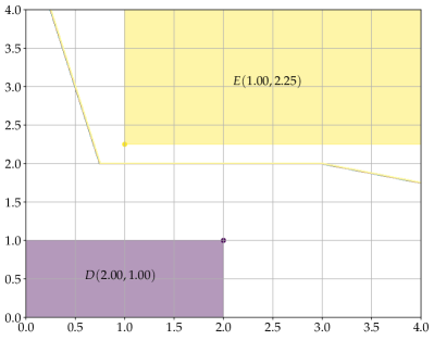
Figure 1: The purple and the yellow regions corresponds respectively to the sets $E(1,2.25)$ and $D(2,1)$. The piece-wise linear curve corresponds to the decision boundary of the DEP classifier with $\beta=0.2$.

In the previous paragraph, we pointed out that erosion-based and dilation-based morphological perceptrons focus respectively on the positive and the negative classes. The dilation-erosion perceptron (DEP) proposed by Araújo allows a graceful balance between the two classes de A. Araújo (2011). The dilation-erosion perceptron is simply a convex combination of an erosion-based and a dilation-based morphological perceptron. In mathematical terms, given $\boldsymbol{m},\boldsymbol{w}\in\mathbb{R}^{n}$ and $0\leq\beta\leq 1$, the decision function of a DEP classifier is defined by

$$\tau(\boldsymbol{x})=\beta\delta_{\boldsymbol{w}}(\boldsymbol{x})+(1-\beta)\varepsilon_{\boldsymbol{m}}(\boldsymbol{x}),\quad\forall\boldsymbol{x}\in\mathbb{R}^{n}.$$ (18)

The binary DEP classifier $\phi:\mathbb{R}^{n}\to\{-1,+1\}$ is defined by the composition

$$\phi=\text{sgn}\tau.$$ (19)

In other words, given $\boldsymbol{m},\boldsymbol{w}\in\mathbb{R}^{n}$ and $\beta\in[0,1]$, the class of an unknown pattern $\boldsymbol{x}\in\mathbb{R}^{n}$ is determined by evaluating $\phi(\boldsymbol{x})=\text{sgn}\tau(\boldsymbol{x})$.

Note that $\tau$ given by (18) corresponds respectively to $\delta_{\boldsymbol{w}}$ and $\varepsilon_{\boldsymbol{m}}$ when $\beta=0$ and $\beta=1$. More generally, the parameter $\beta$ controls the trade off between the dilation-based and the erosion-based morphological perceptrons, which focus on negative and positive classes, respectively. For illustrative purposes, the decision boundary of a DEP classifier obtained by considering $\beta=0.2$, $\boldsymbol{m}=(1,2.25)$ and $\boldsymbol{w}=(2,1)$ is depicted in Figure 1. In this case, the decision boundary of the DEP classifier $\phi$ is closer to the decision boundary of $\text{sgn}\varepsilon_{\boldsymbol{m}}$ than that of $\text{sgn}\delta_{\boldsymbol{w}}$. We address a good choice of the parameter $\beta$ of a DEP classifier in the following subsection. In the following subsection we also review the elegant convex-concave procedure proposed recently by Charisopoulus and Maragos to train the morphological perceptrons $\varepsilon_{\boldsymbol{m}}$ and $\delta_{\boldsymbol{w}}$ Charisopoulos and Maragos (2017).

3.2 Convex-Concave Procedure for Training Morphological Perceptron

In analogy to the soft-margin support vector classifier, the weights of a morphological perceptron can be determined by solving a convex-concave optimization problem Charisopoulos and Maragos (2017); Shen et al. (2016). Precisely, consider a training set $\mathcal{T}=\{(\boldsymbol{x}_{i},d_{i}):i=1,\ldots,m\}$, where $\boldsymbol{x}_{i}\in\mathbb{R}^{n}$ is a training pattern and $d_{i}\in\{-1,+1\}$ is its binary class label for $i=1,\ldots,m$. To simplify the exposition, let $\mathcal{N}$ and $\mathcal{P}$ denote respectively the sets of negative and positive training patterns, that is,

$$\mathcal{N}=\{\boldsymbol{x}_{i}:(\boldsymbol{x}_{i},d_{i})\in\mathcal{T},d_{i}=-1\}\quad\mbox{and}\quad\mathcal{P}=\{\boldsymbol{x}_{i}:(\boldsymbol{x}_{i},d_{i})\in\mathcal{T},d_{i}=+1\}.$$ (20)

Also, let $\psi_{\boldsymbol{u}}$ be the decision function of either an erosion-based or a dilation-based morphological perceptron. In other words, let $\psi_{\boldsymbol{u}}=\varepsilon_{\boldsymbol{m}}$ with $\boldsymbol{u}=\boldsymbol{m}$ or $\psi_{\boldsymbol{u}}=\delta_{\boldsymbol{w}}$ with $\boldsymbol{u}=\boldsymbol{w}$. The vector $\boldsymbol{u}\in\mathbb{R}^{n}$ of either $\psi_{\boldsymbol{u}}=\varepsilon_{\boldsymbol{m}}$ or $\psi_{\boldsymbol{u}}=\delta_{\boldsymbol{w}}$ is defined as the solution of the following convex-concave optimization problem:

$$\mathop{\mbox{minimize}}_{\boldsymbol{u},\boldsymbol{\xi}}\quad J(\boldsymbol{u},\boldsymbol{\xi})=\frac{1}{|\mathcal{N}|}\sum_{i=1}^{|\mathcal{N}|}\nu_{i}^{-}\max\{0,\xi_{i}^{-}\}+\frac{1}{|\mathcal{P}|}\sum_{i=1}^{|\mathcal{P}|}\nu_{i}^{+}\max\{0,\xi_{i}^{+}\}+C\|\boldsymbol{u}-\boldsymbol{r}\|_{1},$$ (21)

subject to $$\psi_{\boldsymbol{u}}(\boldsymbol{x}_{i})\leq\xi_{i}^{-},\quad\forall x_{i}\in\mathcal{N},$$ (22)

$$\psi_{\boldsymbol{u}}(\boldsymbol{x}_{i})\geq-\xi_{i}^{+},\quad\forall\boldsymbol{x}_{i}\in\mathcal{P},$$ (23)

where $C$ is a regularization parameter, $\boldsymbol{r}$ is a reference value for $\boldsymbol{u}$, $\xi_{i}^{-}$ and $\xi_{i}^{+}$ are slack variable and $\nu_{i}^{-}\geq 0$ and $\nu_{i}^{+}\geq 0$ are their penalty weights. As usual, $|\mathcal{N}|$ and $|\mathcal{P}|$ denote the cardinality of $\mathcal{N}$ and $\mathcal{P}$, respectively.

The slack variables $\xi_{i}^{-}$ and $\xi_{i}^{+}$ measure the classification error of negative and positive training patterns weighted by $\nu_{i}^{-}$ and $\nu_{i}^{+}$, respectively. Indeed, the objective function is minimized when all slack variables are non-positive, that is, $\xi_{i}^{-}\leq 0$ and $\xi_{i}^{+}\leq 0$ for all index $i$. On the one hand, a negative training pattern $\boldsymbol{x}_{i}\in\mathcal{N}$ is miss classified if $\psi_{\boldsymbol{u}}(\boldsymbol{x}_{i})>0$. From (22), however, we have $0<\psi_{\boldsymbol{u}}(\boldsymbol{x}_{i})\leq\xi_{i}^{-}$ and, therefore, the objective function is not minimized. On the other hand, if a positive training pattern $\boldsymbol{x}_{i}\in\mathcal{P}$ is miss classified then $0>\psi_{\boldsymbol{u}}(\boldsymbol{x}_{i})\geq-\xi_{i}$. Equivalently, $\xi_{i}>0$ and, again, the objective is not minimized.

The slack variable penalty weights $\nu_{i}$’s have been introduced to deal with the presence of outliers. The following presents a simple weighting scheme proposed by Charisopoulus and Maragos to penalizes training patterns with greater chances of being outliers Charisopoulos and Maragos (2017). Let $\boldsymbol{\mu}^{-}$ and $\boldsymbol{\mu}^{+}$ be the mean of the negative and positive training patterns, that is,

$$\boldsymbol{\mu}^{-}=\frac{1}{|\mathcal{N}|}\sum_{\boldsymbol{x}_{i}\in\mathcal{N}}\boldsymbol{x}_{i}\quad\mbox{and}\quad\boldsymbol{\mu}^{+}=\frac{1}{|\mathcal{P}|}\sum_{\boldsymbol{x}_{i}\in\mathcal{P}}\boldsymbol{x}_{i},$$ (24)

Also, let $\lambda_{i}^{-}$ and $\lambda_{i}^{+}$ be the reciprocal of the distance between $\boldsymbol{x}_{i}$ and either the mean $\boldsymbol{\mu}_{i}^{-}$ or $\boldsymbol{\mu}_{i}^{+}$. In mathematical terms, define

$$\lambda_{i}^{-}=\frac{1}{\|\boldsymbol{x}_{i}-\boldsymbol{\mu}_{i}^{-}\|},\quad\forall\boldsymbol{x}_{i}\in\mathcal{N},\quad\mbox{and}\quad\lambda_{i}^{+}=\frac{1}{\|\boldsymbol{x}_{i}-\boldsymbol{\mu}_{i}^{+}\|},\quad\forall\boldsymbol{x}_{i}\in\mathcal{P}.$$ (25)

Finally, the slack variable weights $\nu_{i}^{-}$ and $\nu_{i}^{+}$ are obtained by scaling $\lambda_{i}^{-}$ and $\lambda_{i}^{+}$ to the interval $(0,1]$ as follows for all indexed $i$:

$$\nu_{i}^{-}=\frac{\lambda_{i}^{-}}{\max_{j}\{\lambda_{j}^{-}\}}\quad\mbox{and}\quad\nu_{i}^{+}=\frac{\lambda_{i}^{+}}{\max_{j}\{\lambda_{j}^{+}\}}.$$ (26)

As to the reference, we recommend respectively $\boldsymbol{r}=-\bigvee\mathcal{N}$ and $\boldsymbol{r}=-\bigwedge\mathcal{P}$ for the synaptic weights $\boldsymbol{w}$ and $\boldsymbol{m}$. In this case, $\delta_{\boldsymbol{w}}$ and $\varepsilon_{\boldsymbol{m}}$ classifies correctly the largest possible number of negative and positive training patterns, respectively. Also, we recommend a small regularization parameter $C$ so that the objective is dominated by the classification error measured by the slack variables. Although in our computational implementation we adopted $C=10^{-2}$, we recommend to fine tune this hyper-parameter using, for example, exhaustive search or a randomized parameter optimization strategy Bergstra and Bengio (2012).

Finally, we propose to train a DEP classifier using a greedy algorithm. Intuitively, the greedy algorithm first finds the best erosion-based and the best dilation-based morphological perceptrons and then it seeks for their best convex combination. Formally, we first solve two independent convex-concave optimization problems formulated using (21)-(23), one to determine the synaptic weight $\boldsymbol{m}$ of the erosion-based morphological perceptron $\varepsilon_{\boldsymbol{m}}$ and the other to compute $\boldsymbol{w}$ of the dilation-based morphological perceptron $\delta_{\boldsymbol{w}}$. Subsequently, we determine the parameter $\beta$ by minimizing the average hinge loss. In mathematical terms, $\beta$ is obtained by solving the constrained convex problem:

$$\mathop{\mbox{minimize}}_{0\leq\beta\leq 1}\;H(\beta)=\sum_{i=1}^{m}\max\left\{0,-d_{i}\big{[}\beta\delta_{\boldsymbol{w}}(\boldsymbol{x}_{i})+(1-\beta)\varepsilon_{\boldsymbol{m}}(\boldsymbol{x}_{i})\big{]}\right\}.$$ (27)

In our computational experiments, we solved the optimization problem (21)-(23) using CVXOPT python package with the DCCP extension for convex-concave programing Shen et al. (2016) and the MOSEK solver. The source-code of the DEP classifier, trained using convex-concave programming and compatible with the scikit-learn API, is available at https://github.com/mevalle/r-DEP-Classifier.

[Ripley Dataset] To illustrate how the DEP classifier works, let us consider the synthetic two-class dataset of Ripley, which is already split into training and test sets Ripley (1996). We would like to recall that each class of Ripley’s synthetic dataset has a known bimodal distribution and the best accuracy score is approximately 0.92. Using the training set with 250 samples, the convex-concave procedure yielded the synaptic weight vectors $\boldsymbol{m}=(0.53,-0.35)$ and $\boldsymbol{w}=(-0.57,-0.64)$ for $\varepsilon_{\boldsymbol{m}}$ and $\delta_{\boldsymbol{w}}$, respectively. Moreover, the convex optimization problem given by (27) yielded the parameter $\beta=0.42$. The accuracy score on the training and test set was respectively $0.88$ and $0.90$. Figure 2a) shows the scatter plot of the test set along with the decision boundary of the DEP classifier. This figure also depicts the regions $E(\boldsymbol{m})$ and $D(\boldsymbol{w})$ for the erosion-based and dilation-based morphological perceptrons.

a) Ripley’s test set	b) Double-moon test set

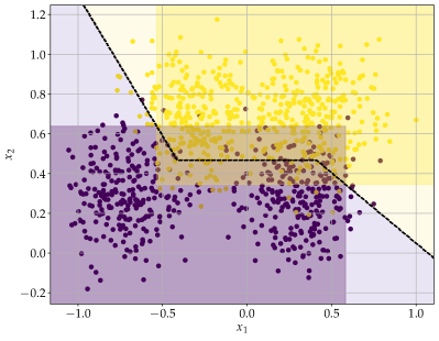
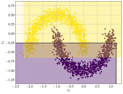
Figure 2: Performance of the DEP classifier on Ripley’s and double-moon datasets described on Examples 3.2 and 2. Scatter plot of test data and the decision boundary of DEP classifier. The purple and the yellow regions corresponds respectively to the sets $D(\boldsymbol{w})$ and $E(\boldsymbol{m})$.

[Double-Moon] In analogy to Haykin’s dooble-moon classification problem, this problem consists of two interleaving half circles which resembles a pair of “moons” facing each other Haykin (2009). Using the command make_moons from python’s scikit-learn API, we generated training and test sets with $1,000$ and $2,000$ pairs of data, respectively. Furthermore, we corrupted both training and test data with Gaussian noise with standard variation $\sigma=0.1$. Figure 2b) shows the test data together with the decision boundary of the DEP classifier and the regions $D(\boldsymbol{w})$ and $E(\boldsymbol{m})$ given respectively by (17) and (16). In this example, the convex-concave procedure yielded the synaptic weight vectors $\boldsymbol{m}=(2.21,0.65)$ and $\boldsymbol{w}=(-1.20,0.25)$. Also, the convex optimization problem (27) yielded $\beta=1$, which means that the DEP classifier $\text{sgn}\tau$ coincides with the dilation-based morphological perceptron $\text{sgn}\delta_{\boldsymbol{w}}$. The DEP classifier yielded an accuracy score of $0.84$ and $0.83$ for training and test sets, respectively.

Despite the DEP classifier yielded satisfactory accuracy scores is test sets from the two previous examples, this classifier has a serious drawback: As a lattice-based classifier, the DEP classifier presupposes a partial ordering on the feature space as well as on the set of classes. From (14), the component-wise ordering given by (1) is adopted in the feature space while the usual total ordering of real-numbers is used to rank the class labels. Most importantly, the DEP classifier $\phi:\mathbb{R}^{n}\to\{-1,+1\}$ defined by the composition (19) is an increasing operator because both sgn and $\tau$ are increasing operators. As a consequence, the patterns from the positive class must be in general greater than the patterns from the negative class. In many practical situations, however, the component-wise ordering of the feature space is not in agreement with the natural ordering of the class labels. For example, if we invert the class labels on the synthetic dataset of Ripley, the accuracy score of the DEP classifier decreases to $0.33$ and $0.31$ for the training and test data, respectively. Similarly, the accuracy score of the DEP classifier decreases respectively to $0.66$ and $0.65$ on training and test set if we invert the class labels in the double-moon classification problem. Fortunately, we can circumvent this drawback through the use of dendrite computations Ritter and Urcid (2003), morphological competitive units Sussner and Esmi (2011), or hybrid morphological/linear neural networks Hernández et al. (2019); Sussner and Campiotti (2020). Alternatively, we can avoid the inconsistency between the partial orderings of the feature and class spaces by making use of multi-valued mathematical morphology.

4 Reduced Dilation-Erosion Perceptron

As pointed out in the previous section, the DEP classifier is an increasing operator $\phi:\mathbb{R}^{n}\to\{-1,+1\}$, where the feature space $\mathbb{R}^{n}$ is equipped with the component-wise ordering given by (1) while the set of classes $\{-1,+1\}$ inherits the natural ordering of real-numbers. In many practical situations, however, the component-wise ordering is not appropriate for the feature space. Motivated by the developments on multi-valued MM, we propose to circumvent this drawback using reduced orderings. Precisely, we introduce the so-called reduced dilation-erosion perceptron (r-DEP) which is a reduced morphological operator derived from (19).

Formally, let us assume the feature space is a vector-valued nonempty set $\mathbb{V}$ and let $\mathcal{C}=\{c_{1},c_{2}\}$ be the set of classes. In practice, the feature space $\mathbb{V}$ is usually a subset of $\mathbb{R}^{n}$, but we may consider more abstract feature sets. Also, let $\mathbb{L}=\bar{\mathbb{R}}^{r}$ and $\mathbb{M}=\{-1,+1\}$ be complete lattices with the component-wise ordering and the natural ordering of real numbers, respectively. Consider the DEP classifier $\phi:\mathbb{L}\to\mathbb{M}$ defined by (19) for some $\boldsymbol{w},\boldsymbol{m}\in\mathbb{R}^{r}$ and $0\leq\beta\leq 1$. Given a one-to-one mapping $\sigma:\mathcal{C}\to\{-1,+1\}$ and a surjective mapping $\rho:\mathbb{V}\to\mathbb{L}$, from Definition 2.2, the mapping $\phi^{r}:\mathbb{V}\to\mathcal{C}$ given by

$$\phi^{r}(\boldsymbol{x})=\sigma^{-1}\Big{(}\phi\big{(}\rho(\boldsymbol{x})\big{)}\Big{)},\quad\forall\boldsymbol{x}\in\mathbb{V},$$ (28)

is an r-increasing morphological operator because $\phi:\mathbb{L}\to\mathbb{M}$ is increasing and the identity $\sigma\phi^{r}=\phi\rho$ holds true. Most importantly, (28) defines a binary classifier $\phi^{r}:\mathbb{V}\to\mathcal{C}$ called reduced dilation-erosion perceptron (r-DEP). The decision function of the r-DEP classifier is the mapping $\tau^{r}:\mathbb{V}\to\bar{\mathbb{R}}$ given by

$$\tau^{r}(\boldsymbol{x})=\beta\delta_{\boldsymbol{w}}\big{(}\rho(\boldsymbol{x})\big{)}+(1-\beta)\varepsilon_{\boldsymbol{m}}\big{(}\rho(\boldsymbol{x})\big{)},\quad\forall\boldsymbol{x}\in\mathbb{V}.$$ (29)

Note that the r-DEP classifier $\phi^{r}$ is obtained from its decision function $\tau^{r}$ by means of the identity $\phi^{r}=\sigma^{-1}\text{sgn}\tau^{r}$.

Simply put, the decision function $\tau^{r}$ of an r-DEP is obtained by composing the surjective mapping $\rho:\mathbb{V}\to\mathbb{L}$ and the decision function $\tau$ of a DEP, that is, $\tau^{r}=\tau\rho$. In other words, $\tau^{r}$ is obtained by applying sequentially the transformation $\rho$ and $\tau$. Thus, given a training set $\mathcal{T}=\{(\boldsymbol{x}_{i},d_{i}):i=1,\ldots,m\}\subset\mathbb{V}\times\mathcal{C}$, we simply train a DEP classifier using the transformed training data

$$\mathcal{T}^{r}=\{(\rho(\boldsymbol{x}_{i}),\sigma(d_{i})):i=1,\ldots,m\}\subseteq\mathbb{R}^{r}\times\{-1,+1\}.$$ (30)

Then, the classification of an unknown pattern $\boldsymbol{x}\in\mathbb{V}$ is achieved by computing $\phi^{r}(\boldsymbol{x})=\sigma^{-1}\text{sgn}\tau\rho(\boldsymbol{x})$.

The major challenge for the design of a successful r-DEP classifier is how to determine the surjective mapping $\rho:\mathbb{V}\to\mathbb{R}^{r}$. Intuitively, the mapping $\rho$ performs a kind of dimensionality reduction which takes into account the lattice structure of patterns and labels. In this paper, we propose to determine $\rho:\mathbb{V}\to\mathbb{R}^{d}$ in a supervised manner. Specifically, based on the successful supervised reduced orderings proposed by Velasco-Forero and Angulo Velasco-Forero and Angulo (2011), we define $\rho:\mathbb{V}\to\mathbb{L}$ using the decision function of support vector classifiers.

Formally, consider a training set $\mathcal{T}=\{(\boldsymbol{x}_{i},d_{i}):i=1,\ldots,m\}\subset\mathbb{V}\times\mathcal{C}$, where $\mathbb{V}\subset\mathbb{R}^{n}$ and $\mathcal{C}=\{c_{1},c_{2}\}$. The mapping $\sigma:\mathcal{C}\to\{-1,+1\}$ is obtained by setting $\sigma(c_{1})=-1$ and $\sigma(c_{2})=+1$. The mapping $\rho:\mathbb{R}^{n}\to\mathbb{R}^{r}$ is defined in a component-wise manner by means of the equation $\rho(\boldsymbol{x})=(\rho_{1}(\boldsymbol{x}),\rho_{2}(\boldsymbol{x}),\ldots,\rho_{r}(\boldsymbol{x}))$, where $\rho_{1},\rho_{2},\ldots,\rho_{r}:\mathbb{R}^{n}\to\mathbb{R}$ are the decision functions of distinct support vector classifiers. Recall that the decision function of a support vector classifier is given by (8). Moreover, the distinct support vector classifiers can be determined using either one of the following approaches referred to as ensemble and bagging:

• Ensemble: The support vector classifiers are determined using the whole training set $\mathcal{T}$ but they have different kernels.

• Bagging: The support vector classifiers have the same kernel and parameters but they are trained using different samples of the training set $\mathcal{T}$.

The following examples, based on Ripley’s and double-moon datasets, illustrate the transformation provided by these two approaches. The following examples also address the performance of the r-DEP classifier.

[Ripley’s Dataset] Consider the synthetic dataset of Ripley Ripley (1996). Using the Gaussian radial basis function (RBF SVC) and the linear SVC (Linear SVC), both with the default parameters of python’s scikit-learn API, we determined the reduced mapping $\rho$ from the training data. Figure 3a) shows the scatter plot of the transformed training set $\mathcal{T}^{r}$ given by (30). Figure 3a) also shows the regions $D(-0.59,-1.28)$ and $E(1.00,0.57)$ and the decision boundary (black-dashed-line) of the DEP classifier on the transformed space. In this example, the convex-concave optimization problem given by (21)-(23) and the minimization of the hinge loss (27) yielded $\boldsymbol{m}=(1.00,0.57)$, $\boldsymbol{w}=(-0.59,-1.28)$, and $\beta=0.54$. Figure 3b) shows the decision boundary of the ensemble r-DEP classifier (black) on the original space together with the scatter plot of the original test set. For comparison purposes, 3b) also shows the decision boundary of the RBF-SVC (blue), linear SVC (green), and the hard-voting classifier (red) obtained using the RBF and linear SVCs. Table 1 contains the accuracy score (between 0 and 1) of each of the classifiers on both training and test sets. Note that the greatest accuracy scores on the test set have been achieved by the r-DEP and the RBF-SVC classifiers. In particular, the r-DEP classifier outperformed the hard-voting ensemble classifier in this example.

a) Ensemble: Ripley’s transformed training set	b) Ensemble: Ripley’s original test set
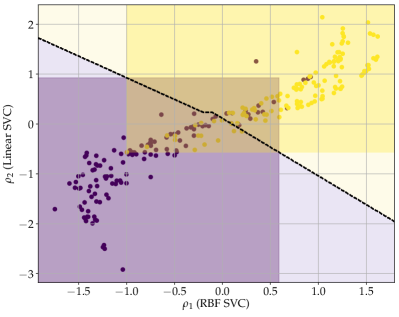
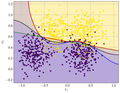
c) Bagging: Ripley’s transformed training set	b) Bagging: Ripley’s original test set

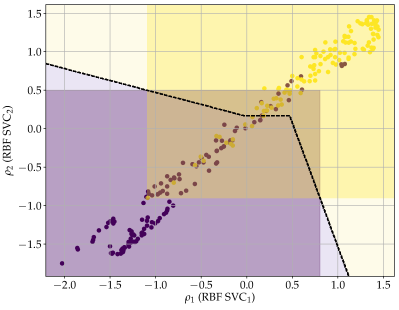
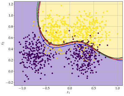
Figure 3: Performance of ensemble and bagging r-DEP classifiers on Ripley’s dataset (see Example 4). a) and c) show the scatter plot of transformed training data, the regions $D(\boldsymbol{w})$ and $E(\boldsymbol{m})$, and the decision boundary of the DEP classifier. b) and d) depict the scatter plot of the original test data and the decision boundary of r-DEP (black) and other binary classifiers.

Table 1: Accuracy score of the classifiers considered in Example 4 on Ripley’s dataset.

Classifier	Training Set	TestSet	Classifier	Training Set	TestSet
Ensemble r-DEP	0.86	0.91	Bagging r-DEP	0.89	0.90
RBF SVC	0.87	0.91	RBF SVC1	0.88	0.91
Linear SVC	0.86	0.89	RBF SVC2	0.88	0.90
Voting SVC	0.87	0.89	Bagging SVC	0.88	0.90

Similarly, we determined the mapping $\rho$ using a bagging of two distinct RBF SVCs trained with different samplings of the original training set. Precisely, we used the default parameters of a bagging classifier (BaggingClassifier) of the scikit-learn but with only two esmitamtors (n_estimators=2) for a visual interpretation of the transformed data. Figure 3c) shows the scatter plot of the training data along with the regions $D(-0.8,-0.5)$ and $E(1.09,0.90)$. In this example, the optimization problem (27) yielded $\beta=0.76$. Figure 3d) shows the scatter plot of the original data and the decision boundaries of the classifiers: bagging r-DEP (black), RBF SVC₁ (blue), RBF SVC₂ (green), and the bagging of the two RBF SVCs (red). Table 1 contains the accuracy score of these four classifiers on both training and test data. Although the RBF SVC₁ yielded the greatest accuracy score in the test set, the bagging r-DEP produced the largest accuracy on the training set. In general, however, the four classifiers are competitive.

[Double-Moon] In analogy to the previous example, we also evaluated the performance of the r-DEP classifier on the double-moon problem presented in Example 2. Figures 4a) and c) show the transformed training set obtained from the mappings determined using the ensemble and bagging strategies, respectively. We considered again a Gaussian RBF and a linear SVC in the ensemble strategy and two Gaussian RBF SVCs for the bagging. Also, we adopted the default parameters of python’s scikit-learn API except for the number of estimators in the bagging strategy which we set to two (n_estimators = 2) for a visual interpretation of the transformed data. Figure 4b) shows the scatter plot of the original test set with the decision boundaries of the ensemble r-DEP (black), RBF SVC (blue), linear SVC (green), and the hard-voting ensemble classifier (red). Similarly, Figure 4d) shows the test data with the decision boundary of the bagging r-DEP (black), RBF SVC₁ (blue), RBF SVC₂ (green), and the bagging classifier (red). Table 2 lists the accuracy score (between 0 and 1) of all the classifiers on both training and test sets of the double-moon problem. As expected, the linear SVC yielded the worst perforamnce. The largest scores have been achieved by both ensemble and bagging r-DEP as well as the Gaussian RBF SVCs and their bagging.

a) Ensemble: Double-moon transformed training set	b) Ensemble: Double-moon original test set
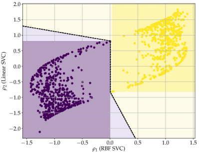
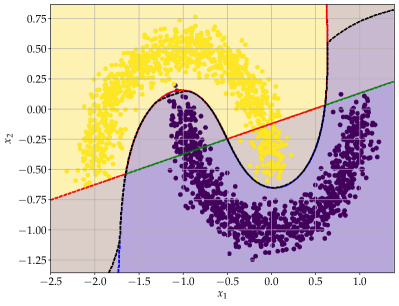
c) Bagging: Double-moon transformed training set	b) Bagging: Double-moon original test set

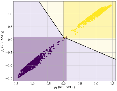
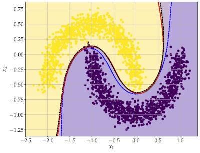
Figure 4: Performance of the ensemble r-DEP classifier on double-moon datasets described on Example 1. a) and c) show the scatter plot of transformed training data, the regions $D(\boldsymbol{w})$ and $E(\boldsymbol{m})$, and the decision boundary of the DEP classifier. b) and d) depict the scatter plot of the original test data and the decision boundary of r-DEP (black) and other binary classifiers.

Table 2: Accuracy score of the classifiers considered in Example 1 on double-moon problem.

Classifier	Training Set	TestSet	Classifier	Training Set	TestSet
Ensemble r-DEP	1.00	1.00	Bagging r-DEP	1.00	1.00
RBF SVC	1.00	1.00	RBF SVC1	1.00	1.00
Linear SVC	0.88	0.88	RBF SVC2	1.00	1.00
Voting SVC	0.93	0.94	Bagging SVC	1.00	1.00

We would like to point out that, in contrast to the original DEP classifier, the perforamance of the r-DEP model remains high if we change the pattern labels. In the following section we provide more conclusive computational experiments concerning the performance of r-DEP for binary classification.

5 Computational Experiments

Let us now provide extensive computational experiments to evaluate the performance of the ensemble and bagging r-DEP classifiers. In the ensemble strategy, the mapping $\rho$ is obtained by considering a RBF SVC, a linear SVC, and a polynomial SVC. The bagging strategy consists of 10 RBF SVCs where each base estimator has been trained using a sampling of the original training set with replacement. Let us also compare the new r-DEP classifiers with the original DEP classifier, linear SVC, RBF SVC, the polynomial SVC (poly SVC) as well as an ensemble of the three SVCs and a bagging of RBF SVCs. We would like to point out that we used the default parameters of the python’s scikit-learn API in our computational experiments Pedregosa et al. (2011); Buitinck et al. (2013).

We considered a total of 30 binary classification problems available on the OpenML repository available at https://www.openml.org/ Vanschoren et al. (2013). We would like to point out that most datasets we considered are also available at the well-known UCI machine learning repository uci . We used the OpenML repository because all the datasets can be accessed by means of the command fetch_openml from python’s scikit-learn Pedregosa et al. (2011). Moreover, we handled missing data using the SimpleImputer command, also from scikit-learn. Table 3 lists the 30 datasets considered. Table 3 also include the number of instances ($\#$instances), the number of features ($\#$features), the percentage of the negative and positive patterns, denoted by the pair $(\mathcal{N}\%,\mathcal{P}\%)$, and the OpenML name/version.

Table 3: Informations on the considered datasets.

	Name	# Instances	# Features	$\mathbf{(\mathcal{N}\%,\mathcal{P}\%)}$	OpenML Name/Version
1	Arsene	200	10000	(44,56)	arcene/1
2	Australian	690	14	(56,44)	Australian/4
3	Banana	5300	2	(55,45)	banana/1
4	Banknote	1372	4	(56,44)	banknote-authentication/1
5	Blood Transfusion	748	4	(76,24)	blood-transfusion-service-center/1
6	Breast Cancer Wisconsin	569	30	(63,37)	wdbc/1
7	Chess	3196	36	(48,52)	kr-vs-kp/1
8	Colic	368	22	(37,63)	colic/2
9	Credit Approval	690	15	(44,56)	credit-approval/1
10	Credit-g	1000	20	(30,70)	credit-g/1
11	Cylinder Bands	540	37	(42,58)	cylinder-bands/2
12	Diabetes	768	8	(65,35)	diabetes/1
13	Egg-Eye-State	14980	14	(55,45)	eeg-eye-state/1
14	Haberman	306	3	(74,26)	haberman/1
15	Hill-Valley	1212	100	(50,50)	hill-valley/1
16	Ilpd	583	10	(71,29)	ilpd/1
17	Internet Advertisements	3279	1558	(14,86)	Internet-Advertisements/2
18	Ionosphere	351	34	(36,64)	ionosphere/1
19	MOFN-3-7-10	1324	10	(22,78)	mofn-3-7-10/1
20	Monks-2	601	6	(66,34)	monks-problems-2/1
21	Mushroom	8124	22	(52,48)	mushroom/1
22	Phoneme	5404	5	(71,29)	phoneme/1
23	Pishing Websites	11055	30	(44,56)	PhishingWebsites/1
24	Sick	3772	29	(94, 6)	sick/1
25	Sonar	208	60	(53,47)	sonar/1
26	Spambase	4601	57	(61,39)	spambase/1
27	Steel Plates Fault	1941	33	(65,35)	steel-plates-fault/1
28	Thoracic Surgery	470	16	(85,15)	thoracic$\_$surgery/1
29	Tic-Tac-Toe	958	9	(35,65)	tic-tac-toe/1
30	Titanic	2201	3	(68,32)	Titanic/2

Note that the number of samples ranges from 200 (Arsene) to 14,980 (Egg-Eye-State) while the number of features varies from 2 (Banana) to 10,000 (Arsene). Furthermore, some datasets such as the Sick and Toracic Surgery are extremely unbalanced. Therefore, we used the balanced accuracy score, which ranges from 0 to 1, to measure the performance of a classifier Brodersen et al. (2010). Table 4 contain the mean and standard deviation of the balanced accuracy score obtained using a stratified $10$-fold cross-validation. The largest mean score for each dataset have been typed using boldface.

We would like to point out that, to avoid biases, we used the same training and test partition for all the classifiers. Also, we pre-processed the data using the command StandardScaler from scikit-learn, that is, we computed the mean and the standard deviation of each feature on the training set and normalized both training and test sets using the obtained values. The StandardScaler transformation has also been applied on the output of the $\rho$ mapping. The source-code of the computational experiment is available at https://github.com/mevalle/r-DEP-Classifier.

From Table 4, the largest average of the balanced accuracy scores have been achieved by the ensemble and bagging r-DEP classifiers. Using paired Student’s t-test with confidence level at 99%, we confirmed that the ensemble and bagging r-DEP, in general, performed better than the other classifiers. In fact, Figure 5 shows the Hasse diagram of the outcome of paired hypothesis tests Burda (2013); Weise and Chiong (2015). Specifically, an edge in this diagram means that the hypothesis test discarded the null hypothesis that the classifier on the top yielded balanced accuracy score less than or equal to the classifier on the bottom. For example, Student’s t-test discarded the null hypothesis that the ensemble r-DEP classifier performs as well as or worst than the hard-voting ensemble of SVCs. In other words, the ensemble r-DEP statistically outperformed the ensemble of SVCs. Concluding, in Figure 5, the method on the top of an edge statistically outperformed the method on the bottom.

Table 4: Average and standard deviation of the balanced accuracy scores obtained from the classifiers using stratified 10-fold cross-validation.

	Linear SVC	RBF SVC	Poly SVC	Ensemble of SVCs	Bagging of SVC	DEP	Ensemble r-DEP	Bagging r-DEP
Arsene	$\mathbf{0.90\pm 0.08}$	0.77$\pm$0.05	0.77$\pm$0.10	0.85$\pm$0.07	0.79$\pm$0.07	0.53$\pm$0.05	0.88$\pm$0.08	0.77$\pm$0.08
Australian	0.86$\pm$0.03	0.86$\pm$0.04	0.84$\pm$0.04	0.85$\pm$0.05	$\mathbf{0.86\pm 0.04}$	0.72$\pm$0.14	0.86$\pm$0.04	0.86$\pm$0.04
Banana	0.50$\pm$0.00	0.90$\pm$0.01	0.61$\pm$0.02	0.63$\pm$0.01	$\mathbf{0.90\pm 0.01}$	0.48$\pm$0.02	0.89$\pm$0.01	0.90$\pm$0.01
Banknote	0.99$\pm$0.01	$\mathbf{1.00\pm 0.00}$	0.99$\pm$0.01	0.99$\pm$0.01	$\mathbf{1.00\pm 0.00}$	0.41$\pm$0.05	$\mathbf{1.00\pm 0.00}$	$\mathbf{1.00\pm 0.00}$
Blood Transfusion	0.50$\pm$0.00	0.56$\pm$0.03	0.53$\pm$0.03	0.53$\pm$0.02	0.55$\pm$0.03	0.55$\pm$0.06	$\mathbf{0.66\pm 0.06}$	0.55$\pm$0.06
Breast Cancer Wisconsin	0.97$\pm$0.02	0.97$\pm$0.02	0.87$\pm$0.03	0.97$\pm$0.01	$\mathbf{0.97\pm 0.02}$	0.88$\pm$0.06	0.97$\pm$0.02	0.97$\pm$0.02
Chess	0.97$\pm$0.01	0.99$\pm$0.01	0.97$\pm$0.01	0.99$\pm$0.01	0.99$\pm$0.01	0.52$\pm$0.03	0.99$\pm$0.01	$\mathbf{0.99\pm 0.01}$
Colic	0.81$\pm$0.07	0.83$\pm$0.07	0.70$\pm$0.05	0.82$\pm$0.07	$\mathbf{0.84\pm 0.08}$	0.56$\pm$0.10	0.81$\pm$0.05	0.82$\pm$0.07
Credit Approval	0.86$\pm$0.04	0.86$\pm$0.04	0.85$\pm$0.05	$\mathbf{0.87\pm 0.05}$	0.86$\pm$0.04	0.55$\pm$0.13	0.79$\pm$0.08	0.85$\pm$0.04
Credit-g	0.67$\pm$0.06	0.67$\pm$0.07	0.61$\pm$0.05	0.66$\pm$0.07	0.67$\pm$0.07	0.55$\pm$0.09	0.69$\pm$0.07	$\mathbf{0.71\pm 0.06}$
Cylinder Bands	0.66$\pm$0.07	0.77$\pm$0.07	0.66$\pm$0.09	0.71$\pm$0.07	0.75$\pm$0.08	0.53$\pm$0.05	$\mathbf{0.79\pm 0.06}$	0.76$\pm$0.09
Diabetes	0.73$\pm$0.07	0.70$\pm$0.07	0.66$\pm$0.05	0.71$\pm$0.06	0.71$\pm$0.06	0.65$\pm$0.05	$\mathbf{0.74\pm 0.05}$	0.72$\pm$0.04
Egg-Eye-State	0.58$\pm$0.02	0.63$\pm$0.05	0.53$\pm$0.01	0.59$\pm$0.03	0.63$\pm$0.05	0.49$\pm$0.03	0.59$\pm$0.03	$\mathbf{0.66\pm 0.04}$
Haberman	0.50$\pm$0.02	0.57$\pm$0.08	0.50$\pm$0.02	0.50$\pm$0.02	0.56$\pm$0.05	0.58$\pm$0.07	$\mathbf{0.60\pm 0.11}$	0.58$\pm$0.12
Hill-Valley	0.61$\pm$0.03	0.50$\pm$0.04	0.53$\pm$0.02	0.58$\pm$0.03	0.50$\pm$0.04	0.52$\pm$0.05	$\mathbf{0.69\pm 0.11}$	0.52$\pm$0.04
Ilpd	0.50$\pm$0.00	0.51$\pm$0.02	0.50$\pm$0.02	0.50$\pm$0.01	0.50$\pm$0.02	0.46$\pm$0.08	$\mathbf{0.63\pm 0.09}$	0.61$\pm$0.09
Internet Advertisements	0.91$\pm$0.04	0.89$\pm$0.02	0.81$\pm$0.04	0.88$\pm$0.03	0.89$\pm$0.03	0.77$\pm$0.08	$\mathbf{0.93\pm 0.03}$	0.89$\pm$0.03
Ionosphere	0.86$\pm$0.06	0.93$\pm$0.04	0.67$\pm$0.07	0.86$\pm$0.07	0.94$\pm$0.04	0.90$\pm$0.07	0.88$\pm$0.05	$\mathbf{0.94\pm 0.02}$
MOFN-3-7-10	$\mathbf{1.00\pm 0.00}$	$\mathbf{1.00\pm 0.00}$	$\mathbf{1.00\pm 0.00}$	$\mathbf{1.00\pm 0.00}$	$\mathbf{1.00\pm 0.00}$	0.57$\pm$0.07	$\mathbf{1.00\pm 0.00}$	$\mathbf{1.00\pm 0.00}$
Monks-2	0.50$\pm$0.00	0.65$\pm$0.06	0.49$\pm$0.02	0.50$\pm$0.01	0.65$\pm$0.06	0.49$\pm$0.03	0.70$\pm$0.06	$\mathbf{0.79\pm 0.04}$
Mushroom	0.98$\pm$0.01	$\mathbf{1.00\pm 0.00}$	$\mathbf{1.00\pm 0.00}$	$\mathbf{1.00\pm 0.00}$	$\mathbf{1.00\pm 0.00}$	0.71$\pm$0.11	$\mathbf{1.00\pm 0.00}$	$\mathbf{1.00\pm 0.00}$
Phoneme	0.72$\pm$0.02	0.81$\pm$0.02	0.65$\pm$0.02	0.74$\pm$0.02	0.81$\pm$0.02	0.74$\pm$0.02	0.82$\pm$0.03	$\mathbf{0.83\pm 0.03}$
Pishing Websites	0.90$\pm$0.01	0.95$\pm$0.01	0.94$\pm$0.01	0.94$\pm$0.01	0.95$\pm$0.01	0.59$\pm$0.10	0.95$\pm$0.01	$\mathbf{0.95\pm 0.01}$
Sick	0.81$\pm$0.06	0.75$\pm$0.02	0.61$\pm$0.04	0.75$\pm$0.05	0.75$\pm$0.03	0.52$\pm$0.04	$\mathbf{0.89\pm 0.03}$	0.88$\pm$0.05
Sonar	0.75$\pm$0.09	0.83$\pm$0.07	0.82$\pm$0.06	0.82$\pm$0.07	0.84$\pm$0.08	0.49$\pm$0.09	0.85$\pm$0.08	$\mathbf{0.87\pm 0.07}$
Spambase	0.92$\pm$0.01	0.93$\pm$0.01	0.73$\pm$0.02	0.93$\pm$0.01	0.93$\pm$0.01	0.51$\pm$0.06	0.93$\pm$0.01	$\mathbf{0.93\pm 0.01}$
Steel Plates Fault	$\mathbf{1.00\pm 0.00}$	1.00$\pm$0.01	1.00$\pm$0.00	$\mathbf{1.00\pm 0.00}$	1.00$\pm$0.01	0.51$\pm$0.02	$\mathbf{1.00\pm 0.00}$	1.00$\pm$0.00
Thoracic Surgery	0.50$\pm$0.00	0.50$\pm$0.00	0.49$\pm$0.02	0.50$\pm$0.00	0.50$\pm$0.00	0.51$\pm$0.10	$\mathbf{0.56\pm 0.12}$	0.50$\pm$0.10
Tic-Tac-Toe	0.50$\pm$0.00	0.86$\pm$0.05	0.74$\pm$0.06	0.74$\pm$0.06	0.87$\pm$0.05	0.61$\pm$0.05	$\mathbf{0.89\pm 0.04}$	0.89$\pm$0.03
Titanic	0.70$\pm$0.03	0.68$\pm$0.02	$\mathbf{0.71\pm 0.03}$	0.71$\pm$0.03	0.69$\pm$0.02	0.43$\pm$0.09	0.60$\pm$0.06	0.70$\pm$0.03
Average	0.76$\pm$0.18	0.80$\pm$0.16	0.73$\pm$0.17	0.77$\pm$0.17	0.80$\pm$0.16	0.58$\pm$0.12	$\mathbf{0.82\pm 0.14}$	0.81$\pm$0.15

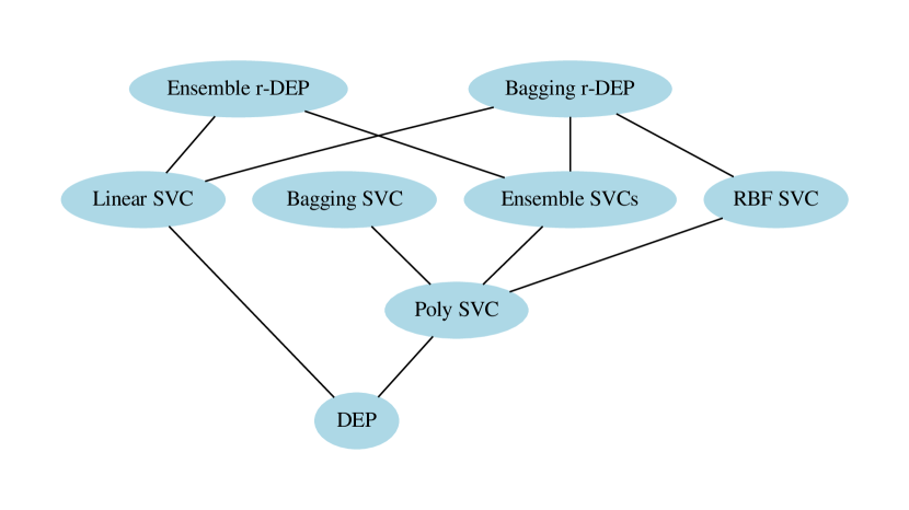
Figure 5: Hasse diagram of paired Student’s t-test with confidence level at 99%.

The outcome of the computational experiment is also summarized on the boxplot shown on Figure 6. The boxplot confirms that the ensemble and bagging r-DEP classifiers yielded, in general, the largest balanced accuracy scores. This boxplot also reveals the poor performance of the DEP classifier which presupposes the positive samples are, in general, greater than or equal to the negative samples according to the component-wise ordering. In particular, the three points above the box of the DEP classifier corresponds to the average balanced accuracy score values 0.90, 0.88, and 0.77 obtained from the datasets Ionosphere, Breast Cancer Wisconsin, and Internet Advertisement, respectively. It turns out, however, that the ensemble and bagging r-DEP classifiers outperformed the original DEP model even in these three datasets. This remark confirms the important role of the transformations $\rho$ and $\sigma$ for successful applications of increasing lattice-based models.

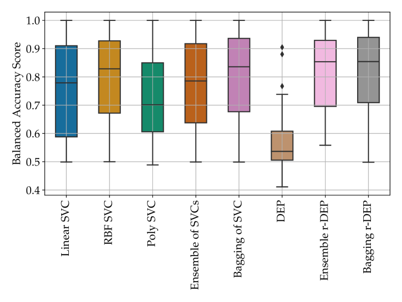
Figure 6: Boxplot summarizing the average balanced accuracy scores provided on Table 4. In general, the ensemble and bagging r-DEP classifiers yielded largest balanced accuracy scores.

6 Concluding Remarks

In analogy to Rosemblatt’s perceptron, the morphological perceptron introduced by Ritter and Sussner can be applied for binary classification Ritter and Sussner (1996). In contrast to the traditional perceptron, however, the usual algebra is replaced by lattice-based operations in the morphological perceptron models. Specifically, the erosion-based and the dilation-based morphological perceptrons compute respectively an erosion $\varepsilon_{\boldsymbol{m}}$ and a dilation $\delta_{\boldsymbol{w}}$ given by (3) followed by the application of the sign function. The erosion-based and dilation-based morfological perceptrons focus respectively on the positive and negative classes. A graceful balance between the two morphological perceptrons is provided by the dilation-erosion perceptron (DEP) classifier whose decision function given by (18) is nothing but a linear combination of the an erosion $\varepsilon_{\boldsymbol{m}}$ and a dilation $\delta_{\boldsymbol{w}}$ de A. Araújo (2011).

In this paper, we propose to train a DEP classifier in two steps. First, based on the works of Charisopoulus and Maragos Charisopoulos and Maragos (2017), the synaptic weights $\boldsymbol{m}$ and $\boldsymbol{w}$ of $\varepsilon_{\boldsymbol{m}}$ and $\delta_{\boldsymbol{w}}$ are determined by solving two independent convex-concave optimization problems given by (21)-(23) Shen et al. (2016). Subsequently, the parameter $\beta$ is determined by minimizing the hinge loss given by (27).

Despite its elegant formulation, as a lattice-based model the DEP classifier presupposes that both feature and class spaces are partially ordered sets. The feature patterns, in particular, are ranked according to the component-wise ordering given by (1). Furthermore, the DEP classifier is an increasing operator. Therefore, it implicitly assumes a relationship between the orderings of features and classes. In many practical situations, however, the component-wise ordering is not appropriate for ranking features. Using results from multi-valued mathematical mophology, in this paper we introduced the reduced dilation-erosion perceptron (r-DEP) classifier. The r-DEP classifier corresponds to the r-increasing morphological operator derived from the DEP classifier $\phi$ by means of (28) using a one-to-one correspondence $\sigma$ between the set of classes $\mathcal{C}$ and $\{-1,+1\}$ and a surjective mapping $\rho$ from the feature space $\mathbb{V}$ to $\bar{\mathbb{R}}^{r}$. Finding appropriate transformation mapping $\rho$ is the major challenge on the design of an r-DEP classifier.

Inspired by the supervised reduced ordering proposed by Velasco-Forero and Angulo Velasco-Forero and Angulo (2011), we defined the transformation mapping $\rho$ using the decision functions of either an ensemble of SVCs with different kernels or a bagging of a base SVC trained using different samples of the original traning set. The source-codes of the ensemble and bagging r-DEP classifiers are available at https://github.com/mevalle/r-DEP-Classifier. Both ensemble and bagging r-DEP classifiers yielded the highest average of the balanced accuracy score among SVCs, their ensemble, and bagging of RBF SVCs, on 30 binary classification problems from the OpenML repository. Furthermore, paired Student’s t-test with significance level at $99\%$ confirmed that the bagging r-DEP classifier outperformed the individual SVCs as well as their ensemble in our computational experiment. The outcome of the computational experiment shows the potential application of the ensemble and bagging r-DEP classifier on practical pattern recognition problems including – but not limited to – credit card fraud detection or medical diagnosis. Moreover, although we only focused on binary classification, multi-class problems can be addressed using one-against-one or one-against-all strategies available, for instance, in the scikit-learn API.

In the future, we plan to investigate further the approaches used to determine the mapping $\rho$. We also intent to study in details the optimization problem used to train a r-DEP classifier.

This research was funded by the São Paulo Research Foundation (FAPESP) under grant number 2019/02278-2 and the National Council for Scientific and Technological Development (CNPq) under grant number 310118/2017-4.

The author declare no conflict of interest. The funders had no role in the design of the study; in the collection, analyses, or interpretation of data; in the writing of the manuscript, or in the decision to publish the results.

References

yes

References

- Lee (2008) Lee, E.A. Cyber Physical Systems: Design Challenges. 2008 11th IEEE International Symposium on Object and Component-Oriented Real-Time Distributed Computing (ISORC), 2008, pp. 363–369. doi:\changeurlcolorblack10.1109/ISORC.2008.25.
- Rajkumar et al. (2010) Rajkumar, R.; Lee, I.; Sha, L.; Stankovic, J. Cyber-physical systems: The next computing revolution. Design Automation Conference, 2010, pp. 731–736. doi:\changeurlcolorblack10.1145/1837274.1837461.
- Shi et al. (2011) Shi, J.; Wan, J.; Yan, H.; Suo, H. A survey of Cyber-Physical Systems. 2011 International Conference on Wireless Communications and Signal Processing (WCSP), 2011, pp. 1–6. doi:\changeurlcolorblack10.1109/WCSP.2011.6096958.
- Derler et al. (2012) Derler, P.; Lee, E.A.; Sangiovanni Vincentelli, A. Modeling Cyber–Physical Systems. Proceedings of the IEEE 2012, 100, 13–28. doi:\changeurlcolorblack10.1109/JPROC.2011.2160929.
- Stojmenovic and Zhang (2015) Stojmenovic, I.; Zhang, F. Inaugural issue of ‘cyber-physical systems’. Cyber-Physical Systems 2015, 1, 1–4. doi:\changeurlcolorblack10.1080/23335777.2015.970764.
- Oztemel and Gursev (2020) Oztemel, E.; Gursev, S. Literature review of Industry 4.0 and related technologies. Journal of Intelligent Manufacturing 2020, 31, 127–182. doi:\changeurlcolorblack10.1007/s10845-018-1433-8.
- Pachidis et al. (2019) Pachidis, T.; Vrochidou, E.; Kaburlasos, V.G.; Kostova, S.; Bonković, M.; Papić, V. Social Robotics in Education: State-of-the-Art and Directions. In Advances in Service and Industrial Robotics; Aspragathos, N.A.; Koustoumpardis, P.N.; Moulianitis, V.C., Eds.; Springer International Publishing, 2019; Vol. 67, pp. 689–700. doi:\changeurlcolorblack10.1007/978-3-030-00232-9_72.
- Zhang et al. (2017) Zhang, Y.; Qiu, M.; Tsai, C.; Hassan, M.M.; Alamri, A. Health-CPS: Healthcare Cyber-Physical System Assisted by Cloud and Big Data. IEEE Systems Journal 2017, 11, 88–95. doi:\changeurlcolorblack10.1109/JSYST.2015.2460747.
- Kaburlasos (2006) Kaburlasos, V.G. Towards a Unified Modeling and Knowledge-Representation based on Lattice Theory; Vol. 27, Computational Intelligence and Soft Computing Applications Series (Studies in Computational Intelligence), Springer-Verlag New York, Inc.: Secaucus, NJ, USA, 2006.
- Kaburlasos and Ritter (2007) Kaburlasos, V.; Ritter, G., Eds. Computational Intelligence Based on Lattice Theory; Springer-Verlag: Heidelberg, Germany, 2007.
- Birkhoff (1993) Birkhoff, G. Lattice Theory, 3 ed.; American Mathematical Society: Providence, 1993.
- Skowron and Stepaniuk (2001) Skowron, A.; Stepaniuk, J. Information granules: Towards foundations of granular computing. International Journal of Intelligent Systems 2001, 16, 57–85. doi:\changeurlcolorblack10.1002/1098-111X(200101)16:1<57::AID-INT6>3.0.CO;2-Y.
- Yao et al. (2013) Yao, J.T.; Vasilakos, A.V.; Pedrycz, W. Granular Computing: Perspectives and Challenges. IEEE Transactions on Cybernetics 2013, 43, 1977–1989. doi:\changeurlcolorblack10.1109/TSMCC.2012.2236648.
- Serra (1982) Serra, J. Image Analysis and Mathematical Morphology; Academic Press: London, 1982.
- Serra (1988) Serra, J. Image Analysis and Mathematical Morphology, Volume 2: Theoretical Advances; Academic Press: New York, 1988.
- Soille (1999) Soille, P. Morphological Image Analysis; Springer Verlag: Berlin, 1999.
- Najman and Talbot (2013) Najman, L.; Talbot, H., Eds. Mathematical Morphology: From Theory to Applications; John Wiley & Sons, Inc.: Hoboken, NJ, USA, 2013. doi:\changeurlcolorblack10.1002/9781118600788.
- Sternberg (1986) Sternberg, S. Grayscale Morphology. Computer Vision, Graphics and Image Processing 1986, 35, 333–355.
- Nachtegael and Kerre (2001) Nachtegael, M.; Kerre, E.E. Connections between binary, gray-scale and fuzzy mathematical morphologies. Fuzzy Sets and Systems 2001, 124, 73–85.
- Sussner and Valle (2008) Sussner, P.; Valle, M.E. Classification of Fuzzy Mathematical Morphologies Based on Concepts of Inclusion Measure and Duality. Journal of Mathematical Imaging and Vision 2008, 32, 139–159.
- Ronse (1990) Ronse, C. Why Mathematical Morphology Needs Complete Lattices. Signal Processing 1990, 21, 129–154.
- Nachtegael et al. (2011) Nachtegael, M.; Sussner, P.; Mélange, T.; Kerre, E. On the role of complete lattices in mathematical morphology: From tool to uncertainty model. Information Sciences 2011, 181, 1971–1988. Special Issue on Information Engineering Applications Based on Lattices, doi:\changeurlcolorblack10.1016/j.ins.2010.03.009.
- Heijmans (1994) Heijmans, H. Morphological Image Operators; Academic Press: New York, NY, 1994.
- Heijmans (1995) Heijmans, H.J.A.M. Mathematical Morphology: A Modern Approach in Image Processing Based on Algebra and Geometry. SIAM Review 1995, 37, 1–36.
- Soille et al. (1993) Soille, P.; Beucher, S.; Rivest, J.F. Morphological gradients. Journal of Electronic Imaging 1993, 2(4), 326–336.
- Angulo (2007) Angulo, J. Morphological colour operators in totally ordered lattices based on distances: Application to image filtering, enhancement and analysis. Computer Vision and Image Understanding 2007, 107, 56–73. Special issue on color image processing.
- Aptoula and Lefèvre (2007) Aptoula, E.; Lefèvre, S. A Comparative Study on Multivariate Mathematical Morphology. Pattern Recognition 2007, 40, 2914–2929.
- Burgeth and Kleefeld (2014) Burgeth, B.; Kleefeld, A. An approach to color-morphology based on Einstein addition and Loewner order. Pattern Recognition Letters 2014, 47, 29–39.
- Burgeth et al. (2019) Burgeth, B.; Didas, S.; Kleefeld, A. A Unified Approach to the Processing of Hyperspectral Images. Mathematical Morphology and Its Applications to Signal and Image Processing; Burgeth, B.; Kleefeld, A.; Naegel, B.; Passat, N.; Perret, B., Eds.; Springer International Publishing: Cham, 2019; pp. 202–214. doi:\changeurlcolorblack10.1007/978-3-030-20867-7_16.
- Lézoray (2016) Lézoray, O. Complete lattice learning for multivariate mathematical morphology. Journal of Visual Communication and Image Representation 2016, 35, 220–235. doi:\changeurlcolorblack10.1016/j.jvcir.2015.12.017.
- Sangalli and Valle (2019) Sangalli, M.; Valle, M.E. Approaches to Multivalued Mathematical Morphology Based on Uncertain Reduced Orderings. Mathematical Morphology and Its Applications to Signal and Image Processing; Burgeth, B.; Kleefeld, A.; Naegel, B.; Passat, N.; Perret, B., Eds.; Springer International Publishing: Cham, 2019; pp. 228–240. doi:\changeurlcolorblack10.1007/978-3-030-20867-7_18.
- Velasco-Forero and Angulo (2014) Velasco-Forero, S.; Angulo, J. Vector Ordering and Multispectral Morphological Image Processing. Advances in Low-Level Color Image Processing; Celebi, M.E.; Smolka, B., Eds.; Springer Netherlands: Dordrecht, 2014; pp. 223–239. doi:\changeurlcolorblack10.1007/978-94-007-7584-8_7.
- Velasco-Forero and Angulo (2011) Velasco-Forero, S.; Angulo, J. Supervised Ordering in : Application to Morphological Processing of Hyperspectral Images. IEEE Transactions on Image Processing 2011, 20, 3301–3308. doi:\changeurlcolorblack10.1109/TIP.2011.2144611.
- Sussner and Esmi (2011) Sussner, P.; Esmi, E.L. Morphological Perceptrons with Competitive Learning: Lattice-Theoretical Framework and Constructive Learning Algorithm. Information Sciences 2011, 181, 1929–1950. doi:\changeurlcolorblack10.1016/j.ins.2010.03.016.
- Ritter and Sussner (1996) Ritter, G.X.; Sussner, P. An Introduction to Morphological Neural Networks. Proceedings of the 13th International Conference on Pattern Recognition; , 1996; pp. 709–717.
- Sussner (1998) Sussner, P. Kernels for Morphological Associative Memories. Proceedings of the International ICSA/IFAC Symposium on Neural Computation; , 1998; pp. 79–85.
- Ritter and Urcid (2003) Ritter, G.X.; Urcid, G. Lattice Algebra Approach to Single-Neuron Computation. IEEE Transactions on Neural Networks 2003, 14, 282–295.
- Sussner and Esmi (2009) Sussner, P.; Esmi, E.L. Introduction to Morphological Perceptrons with Competitive Learning. Proceedings of the International Joint Conference on Neural Networks 2009; , 2009; pp. 3024–3031.
- Pessoa and Maragos (2000) Pessoa, L.; Maragos, P. Neural networks with hybrid morphological/rank/linear nodes: a unifying framework with applications to handwritten character recognition. Pattern Recognition 2000, 33, 945–960.
- de A. Araújo (2011) de A. Araújo, R. A class of hybrid morphological perceptrons with application in time series forecasting. Knowledge-Based Systems 2011, 24, 513 – 529. doi:\changeurlcolorblackhttps://doi.org/10.1016/j.knosys.2011.01.001.
- Hernández et al. (2019) Hernández, G.; Zamora, E.; Sossa, H.; Téllez, G.; Furlán, F. Hybrid neural networks for big data classification. Neurocomputing 2019, p. S0925231219314560. doi:\changeurlcolorblack10.1016/j.neucom.2019.08.095.
- Mondal et al. (2019) Mondal, R.; Santra, S.; Chanda, B. Dense Morphological Network: An Universal Function Approximator, 2019, [1901.00109].
- Franchi et al. (2020) Franchi, G.; Fehri, A.; Yao, A. Deep morphological networks. Pattern Recognition 2020, 102, 107246. doi:\changeurlcolorblack10.1016/j.patcog.2020.107246.
- Arce et al. (2018) Arce, F.; Zamora, E.; Sossa, H.; Barrón, R. Differential evolution training algorithm for dendrite morphological neural networks. Applied Soft Computing 2018, 68, 303–313. doi:\changeurlcolorblack10.1016/j.asoc.2018.03.033.
- Sussner and Campiotti (2020) Sussner, P.; Campiotti, I. Extreme learning machine for a new hybrid morphological/linear perceptron. Neural Networks 2020, 123, 288 – 298. doi:\changeurlcolorblackhttps://doi.org/10.1016/j.neunet.2019.12.003.
- Charisopoulos and Maragos (2017) Charisopoulos, V.; Maragos, P. Morphological Perceptrons: Geometry and Training Algorithms. Mathematical Morphology and Its Applications to Signal and Image Processing; Angulo, J.; Velasco-Forero, S.; Meyer, F., Eds.; Springer International Publishing: Cham, 2017; pp. 3–15. doi:\changeurlcolorblack0.1007/978-3-319-57240-6_1.
- Shen et al. (2016) Shen, X.; Diamond, S.; Gu, Y.; Boyd, S. Disciplined convex-concave programming. 2016 IEEE 55th Conference on Decision and Control (CDC), 2016, pp. 1009–1014. doi:\changeurlcolorblack10.1109/CDC.2016.7798400.
- Vanschoren et al. (2013) Vanschoren, J.; van Rijn, J.N.; Bischl, B.; Torgo, L. OpenML: Networked Science in Machine Learning. SIGKDD Explorations 2013, 15, 49–60. doi:\changeurlcolorblack10.1145/2641190.2641198.
- (49) Matthias Feurer, Jan N. van Rijn, A.K.P.G.N.M.S.R.A.M.J.V.F.H. OpenML-Python: an extensible Python API for OpenML. arXiv, 1911.02490.
- (50) UCI Repository of machine learning databases.
- Heijmans and Ronse (1990) Heijmans, H.J.A.M.; Ronse, C. The algebraic basis of mathematical morphology I. Dilations and erosions. Computer Vision, Graphics, and Image Processing 1990, 50, 245–295. doi:\changeurlcolorblack10.1016/0734-189X(90)90148-O.
- Serra (2009) Serra, J. The “False Colour” Problem. In Mathematical Morphology and Its Application to Signal and Image Processing; Wilkinson, M.H.; Roerdink, J.B., Eds.; Springer Berlin Heidelberg, 2009; Vol. 5720, Lecture Notes in Computer Science, pp. 13–23.
- Goutsias et al. (1995) Goutsias, J.; Heijmans, H.J.A.M.; Sivakumar, K. Morphological Operators for Image Sequences. Computer vision and image understanding 1995, 62, 326–346.
- Vapnik (1998) Vapnik, V.N. Statistical Learning Theory; John Wiley and Sons: New York, NY, USA, 1998.
- Schölkopf and Smola (2002) Schölkopf, B.; Smola, A. Learning with Kernels: Support Vector Machines, Regularization, Optimization, and Beyond; MIT Press: Cambridge, MA, 2002.
- Haykin (2009) Haykin, S. Neural Networks and Learning Machines, 3rd edition ed.; Prentice-Hall: Upper Saddle River, NJ, 2009.
- Ritter et al. (1998) Ritter, G.X.; Sussner, P.; de Leon, J.L.D. Morphological Associative Memories. IEEE Transactions on Neural Networks 1998, 9, 281–293.
- Ritter et al. (1999) Ritter, G.X.; de Leon, J.L.D.; Sussner, P. Morphological Bidirectional Associative Memories. Neural Networks 1999, 6, 851–867.
- Sussner and Valle (2006) Sussner, P.; Valle, M.E. Grayscale Morphological Associative Memories. IEEE Transactions on Neural Networks 2006, 17, 559–570.
- Valle and Sussner (2008) Valle, M.E.; Sussner, P. A General Framework for Fuzzy Morphological Associative Memories. Fuzzy Sets and Systems 2008, 159, 747–768.
- Valle and Sussner (2011) Valle, M.E.; Sussner, P. Storage and Recall Capabilities of Fuzzy Morphological Associative Memories with Adjunction-Based Learning. Neural Networks 2011, 24, 75–90. doi:\changeurlcolorblack10.1016/j.neunet.2010.08.013.
- Santos and Valle (2018) Santos, A.S.; Valle, M.E. Max-plus and min-plus projection autoassociative morphological memories and their compositions for pattern classification. Neural Networks 2018, 100, 84–94. doi:\changeurlcolorblack10.1016/j.neunet.2018.01.013.
- Bergstra and Bengio (2012) Bergstra, J.; Bengio, Y. Random Search for Hyper-Parameter Optimization. Journal of Machine Learning Research 2012, 13, 281–305.
- Ripley (1996) Ripley, B.D. Pattern Recognition and Neural Networks; Cambridge University Press: Cambridge, 1996.
- Pedregosa et al. (2011) Pedregosa, F.; Varoquaux, G.; Gramfort, A.; Michel, V.; Thirion, B.; Grisel, O.; Blondel, M.; Prettenhofer, P.; Weiss, R.; Dubourg, V.; Vanderplas, J.; Passos, A.; Cournapeau, D.; Brucher, M.; Perrot, M.; Duchesnay, E. Scikit-learn: Machine Learning in Python. Journal of Machine Learning Research 2011, 12, 2825–2830.
- Buitinck et al. (2013) Buitinck, L.; Louppe, G.; Blondel, M.; Pedregosa, F.; Mueller, A.; Grisel, O.; Niculae, V.; Prettenhofer, P.; Gramfort, A.; Grobler, J.; Layton, R.; VanderPlas, J.; Joly, A.; Holt, B.; Varoquaux, G. API design for machine learning software: experiences from the scikit-learn project. ECML PKDD Workshop: Languages for Data Mining and Machine Learning, 2013, pp. 108–122.
- Brodersen et al. (2010) Brodersen, K.H.; Ong, C.S.; Stephan, K.E.; Buhmann, J.M. The Balanced Accuracy and Its Posterior Distribution. 2010 20th International Conference on Pattern Recognition, 2010, pp. 3121–3124. doi:\changeurlcolorblack10.1109/ICPR.2010.764.
- Burda (2013) Burda, M. paircompviz: An R Package for Visualization of Multiple Pairwise Comparison Test Results, 2013. doi:\changeurlcolorblack10.18129/B9.bioc.paircompviz.
- Weise and Chiong (2015) Weise, T.; Chiong, R. An alternative way of presenting statistical test results when evaluating the performance of stochastic approaches. Neurocomputing 2015, 147, 235–238. doi:\changeurlcolorblack10.1016/j.neucom.2014.06.071.