Predictions for the CMB from an Anisotropic Quantum Bounce

Abstract

We introduce an extension of the standard inflationary paradigm on which the big bang singularity is replaced by an anisotropic bounce. Unlike in the big bang model, cosmological perturbations find an adiabatic regime in the past. We show that this scenario accounts for the observed quadrupolar modulation in the temperature anisotropies of the cosmic microwave background, and we make predictions for the polarization angular correlation functions $E$-$E$, $B$-$B$ and $E$-$B$, together with temperature-polarization correlations $T$-$B$ and $T$-$E$, that can be used to test our ideas. We base our calculations on the bounce predicted by loop quantum cosmology, but our techniques and conclusions apply to other bouncing models as well.

Introduction. Anisotropies are generic features of homogeneous solutions to Einstein’s equations. This is manifest already for Bianchi I geometries, the simplest anisotropic spacetimes. There, in the absence of anisotropic sources, the contribution of shears to Friedmann equations dilutes with the expansion faster than that of matter and radiation. Therefore, unless anisotropies are exactly zero during the entire history of the cosmos, there must be a time in the past when they were dominant. From this viewpoint, the Friedmann-Lemaître-Robertson-Walker (FLRW) isotropic spacetimes are quite singular. In the standard model of cosmology, one appeals to a phase of slow-roll inflation, when the exponential expansion quickly dilutes anisotropies, and argues that from that time on one can just ignore them. However, the way this argument is applied contains a stronger assumption—that the quantum states describing cosmological perturbations were also isotropic. Anisotropies in quantum fields do not dilute at the same rate as the shears of the homogeneous metric do. In fact, the only reason why they can be washed away is because the cosmic expansion redshifts the wavelengths for which the perturbation fields are anisotropic, potentially shifting them out of the observable Universe. There is no additional dilution agulloparker . However, redshift scales linearly with the expansion, while the dilution of the shear $\sigma^{2}$ scales with its sixth power (in absence of anisotropic sources). Hence, unless inflation is significantly longer than the minimum amount required, one cannot rule out that some anisotropic features were imprinted in the cosmic microwave background (CMB).

This argument, and the fact that the Planck satellite has observed anisotropies in the CMB plnck2018 , has triggered our interest in studying anisotropic extensions of the standard cosmological model. However, within general relativity one finds a major impediment: In a generic anisotropic universe, there are no preferred initial states for the cosmological perturbations. In the theory of inflation, one uses the fact that the wavelengths of the perturbations that we can probe in the CMB were much shorter than the Hubble radius at the onset of slow roll. Then, the notion of adiabatic vacuum can be used to single out an initial quantum state, at least for these wavelengths. However, this argument fails if the preinflationary spacetime is anisotropic (see e.g. ppu-BI1 ). In the absence of preferred initial data, the theory loses predictive power.

This Letter proposes an extension of the standard model, where the big bang singularity is replaced by an anisotropic cosmic bounce. We consider a framework in which the Universe contracts in the remote past, according to Einstein’s theory, until matter and spacetime curvature approach the Planck scale. Then, quantum gravity effects grow and dominate the dynamics, overwhelming the classical attraction and making the Universe bounce. In the far past, the Universe isotropizes and perturbations find an adiabatic regime. Therefore, in this scenario one has preferred initial and final notions of vacua and Hilbert spaces for perturbations. Our goal is to formulate this quantum theory and to solve the evolution, that in the Schrödinger picture reduces to compute the $\mathcal{S}$ matrix between $in$ and $out$ states. We show that perturbations can retain memory of the anisotropic phase of the Universe, and leave an imprint on the CMB, even though anisotropies in the background metric are large only during a short period of time around the bounce. In order to isolate the effects of anisotropies, we work with Bianchi I spacetimes; they differ from spatially flat FLRW spacetimes only by the presence of anisotropic shears.

The classical phase space. Loop quantum cosmology (LQC) uses canonical methods for quantization asrev ; lqc . Therefore, to incorporate perturbations we first need to formulate them in the Hamiltonian language. This task is significantly more tedious and complex than the FLRW counterpart lang , and to the best of our knowledge it has not been developed before (although classical gauge invariant perturbations in Bianchi I have been studied in ppu-BI1 by expanding Einstein’s equations). We follow the geometric approach proposed in gnr . Gauge invariant fields at linear order in perturbations can be obtained by finding a canonical transformation that makes four of the new momenta proportional to each of the four linear constraints of the theory, respectively—the scalar and vector constraints. This guarantees that the conjugate variables to these momenta are pure gauge, while the rest of fields are gauge invariant. The search for such transformation reduces to solving Hamilton-Jacobi-like equations for a generating function. There are multiple solutions, which correspond to different choices of gauge invariant fields. We have selected the choice that in the isotropic limit reduces to the familiar scalar perturbations and the two circularly polarized tensor modes (with helicity $\pm 2$), and denote them by $\Gamma_{0}$ and $\Gamma_{\pm 2}$, respectively.

The dynamics of gauge invariant perturbations is guaranteed to decouple from pure gauge fields, and is generated by a Hamiltonian $\mathcal{H_{\rm pert}}$. Hamilton’s equations can be combined into the second-order differential equations

$$\ddot{\Gamma}_{s}+3\,H\,\dot{\Gamma}_{s}+\frac{k^{2}}{a^{2}}\,\Gamma_{s}+\frac{1}{a^{2}}\,\sum_{s^{\prime}=0}^{2}\,{\cal U}_{ss^{\prime}}\,\Gamma_{s^{\prime}}=0\,,$$ (1)

with $s=0,\pm 2$; we have expanded the fields in Fourier modes $\Gamma_{s}(\vec{k},t)$, and $k$ is the comoving wavenumber. The functions ${\cal U}_{ss^{\prime}}(\vec{k},t)$ are effective potentials made of a complicated combination of the background variables (see aos for details), $a(t)$ is the mean scale factor, and $H=\dot{a}/a$ its Hubble rate. We have implemented this Hamiltonian theory in the symbolic language of Mathematica, and made the code publicly available in math-nb . One important difference with FLRW spacetimes is that the potentials ${\cal U}_{s,s^{\prime}}$ are not diagonal in presence of anisotropies. Therefore, the three fields $\Gamma_{s}$ are coupled and, because these couplings are time dependent, there is no way to diagonalize the equations of motion at all times by means of a local field redefinition.

Quantum theory. The classical phase space we are interested in is the product ${\bf V_{\rm BI}}\times{\bf V_{\rm pert}}$ of Bianchi I geometries and gauge invariant perturbations. At leading order in the perturbations, dynamics is implemented by first determining the evolution within ${\bf V_{\rm BI}}$, and then lifting the dynamical curves to ${\bf V_{\rm pert}}$ with the Hamiltonian $\mathcal{H_{\rm pert}}$. We follow the same strategy in the quantum theory. Namely, the Hilbert space is the product ${\bf H_{\rm BI}}\otimes{\bf H_{\rm pert}}$. ${\bf H_{\rm BI}}$ has been described in awe ; mmwe . A good approximation for quantum states $\Psi_{\rm BI}\in{\bf H_{\rm BI}}$ that at late times are sharply peaked on a classical geometry is provided by the so-called effective equations chiou-vandersloot . These are quantum corrected equations for the directional scale factors and their conjugate variables, whose solutions follow with precision the peak of the wave function $\Psi_{\rm BI}$. The physics of these spacetimes has been studied in detail in gs , and the main features are the following. All solutions contain a bounce of the mean scale factor $a(t)$, which is caused by quantum gravity effects. All strong curvature singularities are resolved, as long as the matter sector satisfies the null energy conditions. Energy densities and shears are bounded from above. Directional scale factors $a_{i}(t)$ bounce generically at different times, giving rise to a richer bounce than in the isotropic case. After the bounce, and in the presence of a scalar field and an inflationary potential $V(\phi)$, Hubble friction slows $\phi$ down and generically leads to a phase of slow roll; such a phase is an attractor in the phase space of this quantum corrected theory gs . In this sense, the bounce provides a mechanism to set up the initial conditions for inflation to occur. Once inflation starts, the scenario provided by the standard cosmological model goes through, with the important difference that the state of perturbations is different from the standard ansatz of the Bunch-Davies vacuum.

We assume the matter content to be a scalar field with a potential $V(\phi)$. In the scenarios of interest (see below) the potential is subdominant in the preinflationary phase, and consequently the generation of anisotropies is independent of $V(\phi)$. For the sake of simplicity, we use $V(\phi)=1/2\,m^{2}\phi^{2}$ and comment below on the effect of other choices. The other freedoms in our predictions come from the choice of an effective Bianchi I quantum spacetime. One such geometry is singled out by specifying the value of the shear squared $\sigma^{2}(t_{B})$, the shear in one of the principal directions, say $\sigma_{x}(t_{B})$, the value of the scalar field $\phi(t_{B})$, and the sign of its time derivative, all at the time $t_{B}$ of the bounce. $\sigma^{2}(t_{B})$ measures the total amount of anisotropies at $t_{B}$; $\sigma_{x}(t_{B})$ indicates the way these anisotropies are distributed in the three principal directions, and $\phi(t_{B})$ and the sign of $\dot{\phi}(t_{B})$ control the number $N$ of $e$-folds of expansion from the bounce to the end of inflation [$\sigma^{2}(t_{B})$ also affects this number, but in a subleading manner gs .

To quantize the perturbations, we follow the conceptual framework introduced in akl ; aan ; hyb and extend it to Bianchi I geometries. We obtain that the dynamics of quantum perturbations $\hat{\Gamma}_{0}$, $\hat{\Gamma}_{\pm 2}$ are described by the equations (1), with the background geometry given by a solution to the effective equations of LQC. The main difficulty arises from the interactions among the quantum fields $\hat{\Gamma}_{0}$, $\hat{\Gamma}_{\pm 2}$, induced by the anisotropies. To describe dynamics, we first define the $in$ and $out$ Hilbert spaces. The former is defined from an adiabatic vacuum in the past (see Sec. IV in aos and aos2 for details), that we take to be anytime before $10000$ Planck times prior to the bounce. At this time, anisotropies are already negligible in the geometries that we have explored, and all Fourier modes of interest are well inside the Hubble radius. The $out$ Fock space is the standard one built from the Bunch-Davies vacuum during inflation, when the anisotropies of the spacetime are negligible again. The quantum evolution is implemented by the $\mathcal{S}$ matrix, which provides a unitary map between the $in$ and $out$ Fock spaces aa . Its action on the $in$ vacuum produces

$$\hat{\mathcal{S}}|in\rangle=$$ (2)

$$\bar{N}\,\bigotimes_{\vec{k}}\exp{\Big{[}\sum_{s,s^{\prime}=0,\pm 2}{\rm V}_{ss^{\prime}}(\vec{k})\,\hat{a}^{out\,\dagger}_{s}(\vec{k})\ \hat{a}^{out\,\dagger}_{s^{\prime}}(-\vec{k})\Big{]}}\,|out\rangle\,,$$

where $\bar{N}$ is a normalization factor, and $V_{ss^{\prime}}(\vec{k}):=\sum_{s^{\prime\prime}}\frac{1}{2}\,\beta^{*}_{s^{\prime\prime}s}\,(\alpha^{-1})^{*}_{s^{\prime}s^{\prime\prime}}$, with $\alpha_{ss^{\prime}}(\vec{k})$ and $\beta_{ss^{\prime}}(\vec{k})$ the Bogoliubov coefficients that relate the $in$ and $out$ vacua. They encode the information of the evolution of perturbations across the anisotropic bounce, and can be computed from the classical equations of motion. The operators $\hat{a}^{out\,\dagger}_{s}$, with $s=0,\pm 2$, create quanta of the familiar scalar and tensor modes in inflation, respectively. The right-hand side of (2) is the product of squeezing operators acting on $|out\rangle$. Consequently, the $in$ vacuum evolves to a state made of entangled pairs of quanta, one with wave number $\vec{k}$ and the other with $(-\vec{k})$; i.e., no net momentum is created. In the isotropic limit $V_{ss^{\prime}}$ becomes diagonal, and the operator in (2) becomes the product of operators for scalar and each of the two tensor modes. This is not the case in presence of anisotropies, where the final state contains entanglement among the three types of perturbations. One can compute, e.g., the entanglement entropy, from the Bogoliubov coefficients aos .

Constraints from observations. We next analyze Planck’s observations of a quadrupolar direction-dependent modulation in the CMB plnck2018 . Since our goal is to describe the largest possible signal that we can expect in the CMB, we choose $\sigma^{2}(t_{B})$ close to its upper bound, and derive the constraints from observations on the other parameters that specify the spacetime geometry. Observations translate to a lower bound for the number of $e$-folds $N$, which keeps anisotropies in the CMB below the observed threshold. On the other hand, if this number happens to be very large, all anisotropies in perturbations would be red-shifted out of the observable Universe. A representative example of our analysis is obtained by choosing $\sigma^{2}(t_{B})=5.78$ in natural units (this is half of its upper bound gs ) and $\sigma_{x}(t_{B})=0$. We have computed the quadrupolar modulation and compared it with data from Planck (see Fig. 1). The result of this analysis is a lower bound for $N$ of $70.1$. Interestingly, this value is compatible with the results found in barrau for the preferred value of $N$ in anisotropic LQC. As we will shortly see, $N=70.1$ is not large enough to wash away all anisotropies in the CMB.

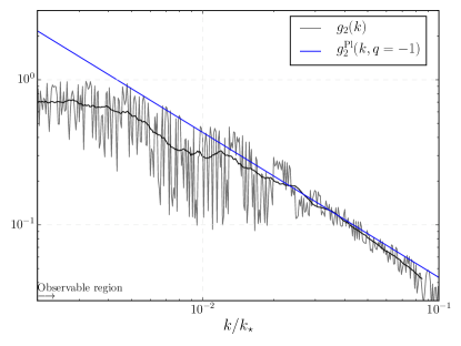
Figure 1: Amplitude of the quadrupolar modulation $g_{2}(k)\equiv\sqrt{\sum_{M}|g_{2M}|^{2}/5}$ of the primordial scalar power spectrum ${\mathcal{P}}(\vec{k})$, where $g_{2M}(k)=\frac{1}{\bar{\mathcal{P}}(k)}\int d\Omega_{\vec{k}}\,{\mathcal{P}}(\vec{k})\,Y^{*}_{2M}(\hat{k})$, with $\bar{\mathcal{P}}(k)\equiv\int d\Omega_{\vec{k}}\,{\mathcal{P}}(\vec{k})$. Planck’s results plnck2018 for the amplitude of a quadrupole that falls off with $k$ as $g^{\rm Pl}_{2}(k)=g^{\rm Pl}_{2}\times(k/k_{\star})^{q}$, for $q=-1$, is shown in blue. The gray line shows our results for a set of individual values of $k$. The outcome oscillates with high frequency around the mean value, shown in black. These oscillations do not show up in angular correlation functions, since they get effectively averaged out when integrating in $k$. $k_{\star}$ is a reference wave number, whose physical value today is $0.05\,{\rm Mpc}^{-1}$. This plot is obtained for $\sigma^{2}(t_{B})=5.78$ and $\sigma_{x}=0$ in natural units, and $N=70.1$.

Predictions for the CMB. We compute the angular correlation functions $C_{\ell\ell^{\prime},mm^{\prime}}^{X,X^{\prime}}\equiv\left\langle a_{\ell m}^{X}a_{\ell^{\prime}m^{\prime}}^{X^{\prime}}\right\rangle$, with

$$a^{X}_{\ell m}=\int d\Omega\,X(\hat{n})\,Y^{*}_{\ell m}(\hat{n})\,,$$ (3)

where $X=T,E,B$ represents the temperature, electric and magnetic components of the polarization, respectively, of the anisotropies in the CMB.

(i) Temperature-Temperature ($T$-$T$). Our theory is invariant under translations and parity, but not under rotations. Parity invariance restricts $C_{\ell\ell^{\prime},mm^{\prime}}^{T,T}$ to vanish unless $\ell+\ell^{\prime}$ is even (isotropy would have also imposed $\ell=\ell^{\prime}$, $m=-m^{\prime}$). We plot in Fig. 2 $C_{\ell}^{TT}\equiv\frac{1}{2\ell+1}\sum_{m=-\ell}^{\ell}(-1)^{m}C_{\ell\ell,m-m}^{TT}$, and compare it with the predictions of isotropic inflation. As expected, the effects of the preinflationary physics are larger for low multipoles (large angular scales) and translate to a modest enhancement of power, although small when compared to uncertainties coming from cosmic variance. Therefore, anisotropies do not alter significantly the best-fit value of the six free parameters of the standard (Lambda cold dark matter) model. We have checked this by running a Markov chain Monte Carlo analysis lewis , using $TT$, $EE$, and $TE$ data planckdata . In contrast, correlation functions for $\ell\neq\ell^{\prime}$ are a smoking gun for anisotropies peloso . In Fig. 2 we also show one of them, namely $C_{\ell\ell+2,00}^{TT}$, as an illustrative example. Other values of $\ell,\ell^{\prime},m,m^{\prime}$ produce similar results. Our result for $C_{\ell\ell+2,00}^{TT}$ is in agreement with the quadrupolar modulation observed by Planck.

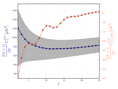
Figure 2: Left axis: Temperature-temperature angular correlation function $C_{\ell}^{TT}$ (dotted blue line). For comparison, the shaded region shows the values obtained from isotropic inflation, including the uncertainties originated from cosmic variance. Right axis: $C_{\ell\ell+2,00}^{TT}$ (red line with squares) (the isotropic counterpart is exactly zero).

(ii) $E$-$E$, $B$-$B$, and $T$-$E$ correlations. The conclusions are similar to the $T$-$T$ case. Namely, these correlations are different from zero only for $\ell+\ell^{\prime}$ even, and the main departures from the isotropic model appear for low multipoles and for $\ell\neq\ell^{\prime}$. As an example, we plot in Fig. 3 $C_{\ell}^{BB}\equiv\frac{1}{2\ell+1}\sum_{m=-\ell}^{\ell}(-1)^{m}C_{\ell\ell,m-m}^{BB}$ and $C_{\ell\ell+2,00}^{BB}$. The latter has an important contribution from the entanglement between tensor perturbations with different polarizations.

(iii) $T$-$B$ and $E$-$B$. Because the $B$-polarization field is a pseudoscalar, while $T$ and $E$ are parity even, these correlations vanish in a parity invariant theory unless $\ell+\ell^{\prime}$ is odd. Since isotropy would also imply $\ell=\ell^{\prime}$, all these correlations vanish in the standard cosmological model. Fig. 4 shows $C_{\ell\ell+1,00}^{T,B}$ and $C_{\ell\ell+1,00}^{E,B}$ in our model. They originate exclusively from the entanglement between scalar and the two tensor modes.

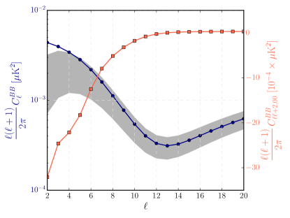
Figure 3: Left axis: $B$-$B$ polarization angular correlation function $C_{\ell}^{BB}$ (dotted blue line), and the predictions from isotropic inflation with cosmic variance (shaded region), for comparison. Right axis: Off-diagonal component of the $B$-$B$ polarization correlation function $C_{\ell\ell+2,00}^{BB}$ (red line with squares).

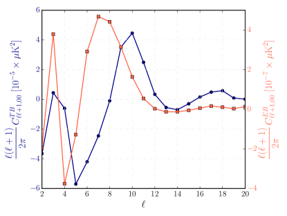
Figure 4: $T$-$B$ (left axis, dotted blue line), and $E$-$B$ (right axis, red line with squares) correlation functions for $\ell^{\prime}=\ell+1$, and $m=0=m^{\prime}$. The isotropic counterpart is identically zero.

In the standard theory of inflation the amplitude of tensor perturbations depends on the choice of $V(\phi)$. This freedom remains in our model. We have chosen the parameters in $V(\phi)$ that best fits existing data, but a different choice of $V(\phi)$ would change the amplitude of $B$-modes. Our invariant prediction for them is, therefore, the magnitude of anisotropies relative to their overall amplitude.

The computational difficulty of these calculations comes from the need to resolve the angular dependence of the primordial power spectra $\mathcal{P}_{s,s^{\prime}}(\vec{k})$ or, equivalently, to decompose $\mathcal{P}_{s,s^{\prime}}(\vec{k})$ in spherical harmonics with spin weight $s-s^{\prime}$. This is a demanding task—the calculation of these plots takes about a week on a 96-core high performance computer (we use the numerical library num-lib ).

Our analysis shows that the quadrupolar modulation of the $T$-$T$ spectrum observed by Planck plnck2018 could be a remnant from an anisotropic pre-inflationary phase, rather than a statistical fluke. Furthermore, we predict that this modulation comes together with concrete effects in the $E$-$E$, $T$-$E$, $B$-$B$, $T$-$B$ and $E$-$B$ correlation functions, which provide a way to test our ideas (further details omitted here can be found in aos2 ).

Discussion. The merits of this Letter are as follows: (i) To introduce a Hamiltonian formulation of gauge invariant perturbations in Bianchi I spacetimes, and to implement the mathematical framework in a publicly available computational algorithm math-nb ; num-lib ; xart . (ii) To formulate an exact quantization of the coupled system of linear perturbations, and to use this formalism to compute the entanglement between scalar and tensor perturbations that anisotropies generate. (iii) To embed this theory within a quantization of the Bianchi I geometry, extending in this way previous studies on quantum cosmology to anisotropic scenarios, a task that has remained elusive due to the complexity of the system. (iv) To show that perturbations can retain memory of the preinflationary universe, although the anisotropies in the background geometry quickly dilute during inflation. This memory is codified in the form of anisotropic correlation functions and quantum entanglement between the different types of perturbations. (v) Finally, and most importantly, we have explained a possible origin for the nonzero quadrupolar modulation observed by Planck, and made concrete predictions for $E$-$E$, $B$-$B$, $T$-$E$, $T$-$B$ and $E$-$B$ correlations in the CMB. Although Planck’s observations of the $T$-$T$ quadrupole alone are not significant enough to declare the detection of anisotropic physics, a detailed search for the effects we describe in the $E$-$E$, $T$-$E$ correlations (that Planck has already partially done), and particularly in $B$ polarization, could boost the significance of the detection. Some of the values we predict, particularly the ones involving $T$-$B$ and $E$-$B$ correlations, are small and probably difficult to observe, but others are not, and could be measured by the next generation of CMB polarization observatories, such as CORE core .

Furthermore, although we have worked within loop quantum cosmology, we expect our conclusions to be valid for other theories that predict a similar bounce (see, e.g., Mukhanov ; 6 ; Shtanov:2002mb ).

Acknowledgements.

- (1) I. Agullo and L. Parker, Phys. Rev. D 83, 063526 (2011); Gen. Rel. Grav. 43, 2541-2545 (2011).
- (2) Planck Collaboration, Planck 2018 results. X. Constraints on inflation, arXiv:1807.06211 (2018).
- (3) T. S. Pereira, C. Pitrou and J. P. Uzan, JCAP 0709, 006 (2007); C. Pitrou, T. S. Pereira, and J. P. Uzan, JCAP 0804, 004 (2008); Comptes rendus - Physique 16, 1027-1037 (2015).
- (4) A. Ashtekar and P. Singh, Class. Quant. Grav. 28, 213001 (2011).
- (5) I. Agullo and P. Singh, Loop Quantum Cosmology: A brief review, in “Loop quantum Gravity: the first 30 years”, Edited by A. Ashtekar and J. Pullin, World Scientific (2017).
- (6) D. Langlois, Class. Quant. Grav. 11, 389 (1994).
- (7) J. Goldberg, E. T. Newman, and C. Rovelli, J. Math. Phys. 32, 2739 (1991).
- (8) I. Agullo, J. Olmedo and V. Sreenath, Phys. Rev. D 101, 123531 (2020).
- (9) J. Olmedo, I. Agullo and V. Sreenath, http://bitbucket.org/jolmedo/bianchii-perts/src/master/ (2019).
- (10) A. Ashtekar, and E. Wilson-Ewing, Phys. Rev. D 79, 083535 (2009).
- (11) M. Martín-Benito, G. A.Mena Marugán, E. Wilson-Ewing, Phys. Rev. D 82, 084012 (2010).
- (12) D. Chiou and K. Vandersloot, Phys. Rev. D 76, 080415 (2007).
- (13) B. Gupt, P. Singh, Phys. Rev. D 86, 024034 (2012), Class. Quant. Grav. 30, 145013 (2013).
- (14) A. Ashtekar, W. Kaminski and J. Lewandowski, Phys. Rev. D 79, 064030 (2009).
- (15) I. Agullo, A. Ashtekar and W. Nelson, Phys. Rev. D 87, 043507 (2013); Class. Quant. Grav. 30, 085014 (2013); Phys. Rev. Lett. 109, 251301 (2012).
- (16) M. Fernández-Méndez, G. A. Mena Maruán and J. Olmedo, Phys. Rev. D 86, 024003 (2012); Phys. Rev. D 88, 044013 (2013); L. Castelló Gomar, M. Fernández-Méndez, G. A. Mena Marugán and J. Olmedo, Phys. Rev. D 90, 064015 (2014); F. Benítez Martínez and J. Olmedo, Phys. Rev. D 93, 124008 (2016).
- (17) I. Agullo, J. Olmedo and V. Sreenath, Observational consequences of Bianchi I spacetimes in loop quantum cosmology, arXiv:2006.01883.
- (18) I. Agullo, and A. Ashtekar, Phys. Rev. D 12, 124010 (2015).
- (19) K. Martineau, A. Barrau, S. Schander, Phys. Rev. D 95, 083507 (2017).
- (20) A. Lewis and S. Bridle, Phys. Rev. D 66, 103511 (2002).
- (21) N. Aghanim et al. (Planck) (2019), 1907.12875.
- (22) A.E. Gumrukcuoglu, A. Himmetoglu, M. Peloso Phys. Rev. D 81, 063528 (2010).
- (23) J. Olmedo, I. Agullo and V. Sreenath, http://bitbucket.org/jolmedo/cosmo-perts/src/master/ (2019).
- (24) I. Agullo, J. Olmedo and V. Sreenath, Mathematics 8, 2, 290 (2020).
- (25) http://www.core-mission.org
- (26) A. H. Chamseddine and V. Mukhanov, JCAP 1703, 009 (2017).
- (27) D. Langlois, H. Liu, Karim Noui, and E. Wilson-Ewing, Class. Quant. Grav. 34, 225004 (2017).
- (28) Y. Shtanov and V. Sahni, Phys. Lett. B 557, 1-6 (2003).