Adapted gauge to a quasilocal measure of the black holes recoil

Abstract

We explore different gauge choices in the moving puncture formulation in order to improve the accuracy of a linear momentum measure evaluated on the horizon of the remnant black hole produced by the merger of a binary. In particular, motivated by the study of gauges in which $m\eta$ takes on a constant value, we design a gauge via a variable shift parameter $m\eta(\vec{r}(t))$. This new parameter takes a low value asymptotically, as well as at the locations of the orbiting punctures, and then takes on a value of approximately 2 at the final hole horizon. This choice then follows the remnant black hole as it moves due to its net recoil velocity. We find that this choice keeps the accuracy of the binary evolution. Furthermore, if the asymptotic value of the parameter $m\eta$ is chosen about or below 1.0, it produces more accurate results for the recoil velocity than the corresponding evaluation of the radiated linear momentum at infinity, for typical numerical resolutions. Detailed studies of an unequal mass $q=m_{1}/m_{2}=1/3$ nonspinning binary are provided and then verified for other mass ratios $(q=1/2,1/5)$ and spinning $(q=1)$ binary black hole mergers.

I Introduction

The discovery by numerical relativity computations Campanelli et al. (2007a); González et al. (2007); Campanelli et al. (2007b) that binary black hole mergers may impart thousand of kilometers per second speeds to the final black hole remnant had an immediate impact on the interest of observational astrophysics to search for signatures of such recoil for supermassive black holes in merged galaxies (See Komossa (2012), for an early review). The interest in searching for observational effects extends to nowadays Chiaberge et al. (2017); Lousto et al. (2017); Chiaberge et al. (2018), including its incidence in statistical distributions Lousto et al. (2010a); Fishbach et al. (2017); Lousto et al. (2012) and binary formation channels as well as cosmological consequences Rodriguez et al. (2018).

More recently theoretical explorations evaluate the possibility to directly detect the effects of recoil on the gravitational waves observed by LIGO Lousto and Healy (2019) and LISA Sesana et al. (2009); Gerosa and Moore (2016). The use of numerical relativity waveforms to directly compare with the observation of gravitational waves require accurate modeling and good coverage of the parameter space Abbott et al. (2016a). There are already successful descriptions for the GW150914 Lovelace et al. (2016); Healy et al. (2019) and GW170104Healy et al. (2018a) events and the analysis of the rest of the O1/O2 events Abbott et al. (2019a) is well underway (Healy et al. 2020a, paper in preparation).

The accurate modeling of the final remnant of the merger of binary black holes is also of high interest for applications to gravitational waves modeling and tests of gravity as a consistency check Abbott et al. (2016b, 2019b). The computation of the final remnant mass and spin can be performed in three independent ways, a fit to the quasinormal modes of the final remnant Kerr black hole Echeverría (1989); Berti et al. (2006, 2009), a computation of the energy and angular momentum carried away by the gravitational radiation to evaluate the deficit from the initial to final mass and spins, and a quasilocal computation of the horizon mass and spin using the isolated horizon formulas Dreyer et al. (2003a). Comparison of the three methods has been carried out in Dain et al. (2008); Lousto and Healy (2019), concluding that at the typical resolutions used in production numerical relativity simulations the horizon quasilocal measures are an order of magnitude more accurate than the radiation or quasinormal modes fittings.

This leads to very accurate modeling of the final mass and spins from their initial binary parameters. In particular for nonprecessing binaries, the modeling Healy and Lousto (2018) warrants errors typically $0.03\%$ for the mass and $0.16\%$ for the spin. Meanwhile the modeling of the final recoils leads to errors of the order of $5\%$ since radiation of linear momentum is used to evaluate them. A similar accurate modeling of the recoil could be attempted by the use of a horizon quasilocal measure.

In reference Krishnan et al. (2007) a quasi-local formula for the linear momentum of black-hole horizons was proposed, inspired by the formalism of quasi-local horizons. This formula was tested using two complementary configurations: (i) by calculating the large orbital linear momentum of the two black holes in an orbiting, unequal-mass, zero-spin, quasi-circular binary and (ii) by calculating the very small recoil momentum imparted to the remnant of the head-on collision of an equal-mass, anti-aligned-spin binary. The results obtained were consistent with the horizon trajectory in the orbiting case, and consistent with the radiated linear momentum for the much smaller head-on recoil velocity. A key observation we will explore in this paper is the dependence of the accuracy on a gauge parameter used in our simulations.

This paper is organized as follows, In Section II we study in detail the effects of choosing different (constant) values of $\eta$, the damping parameter in the shift evolution equation on the accuracy of the quasilocal measure of the horizon linear momentum proposed in Krishnan et al. (2007). We discuss in detail a prototype case of a nonspinning $q=1/3$ binary. Other unequal mass cases and one spinning case are verified as well. In Section III, we perform additional studies of the shift evolution equation for the alternative $\partial_{0}$-gauge, variable $\eta$, and apply what we learned in the previous section to develop a variable shift parameter $\eta$ and to more extreme unequal mass binary black hole mergers. In Section IV we discuss the benefits of the using of different values of $\eta$ from our standard $\eta=2$ (See also van Meter et al. (2006)) for generic simulations, in particular for those that involve an accurate computation of the remnant recoil and we also conclude by noting the advantage of keeping the $\partial_{t}$-gauge for evolutions over the $\partial_{0}$-gauge.

II Numerical Techniques

Since the 2005 breakthrough work Campanelli et al. (2006) We obtain accurate, convergent waveforms and horizon parameters by evolving the BSSNOK Nakamura et al. (1987); Shibata and Nakamura (1995); Baumgarte and Shapiro (1998) system in conjunction with a modified 1+log lapse and a modified Gamma-driver shift condition Alcubierre et al. (2003); Campanelli et al. (2006),

$$\partial_{0}\alpha=(\partial_{t}-\beta^{i}\partial_{i})\alpha = -2\alpha K,$$ (1)

$$\partial_{t}\beta^{a} = \frac{3}{4}\tilde{\Gamma}^{a}-\eta(x^{k},t)\,\beta^{a}.$$ (2)

with an initial vanishing shift and lapse $\alpha(t=0)=2/(1+\psi_{BL}^{4})$. Here, and for the remainder of the paper, latin indices cover the spatial range $i=1,\cdots,3$.

An alternative moving puncture evolution can be achieved Baker et al. (2006) by choosing van Meter et al. (2006)

$$\partial_{0}\alpha=(\partial_{t}-\beta^{i}\partial_{i})\alpha = -2\alpha K,$$ (3)

$$\partial_{0}\beta^{a}=(\partial_{t}-\beta^{i}\partial_{i})\beta^{a} = \frac{3}{4}\tilde{\Gamma}^{a}-\eta(x^{k},t)\,\beta^{a}.$$ (4)

In the subsequent, we will refer to this first order equations for the shift (2) as the $\partial_{t}$-gauge and to (4) as the $\partial_{0}$-gauge. Unless otherwise stated, all binary black hole simulations in this paper use the $\partial_{t}$ gauge.

The parameter $\eta$ (with dimension of one-over-mass: $1/m$) in the shift equation regulates the damping of the gauge oscillations and is commonly chosen to be of order unity (we use $\eta=2/m$) as a compromise between the accuracy and stability of binary black hole evolutions. We have found in Lousto and Zlochower (2008) that coordinate dependent measurements, such as spin and linear momentum direction, become more accurate as $\eta$ is reduced (and resolution $h\to 0$). However, if $\eta$ is too small $(\eta\ll 1/m)$, the runs may become unstable. Similarly, if $\eta$ is too large $(\eta\gg 10/m)$, then grid stretching effects can cause the remnant horizon to continuously grow, eventually leading to an unacceptable loss in accuracy at late times.

We use the TwoPunctures Ansorg et al. (2004) thorn to compute initial data. We evolve these black-hole-binary data-sets using the LazEv Zlochower et al. (2005) implementation of the moving puncture formalism Campanelli et al. (2006). We use the Carpet Schnetter et al. (2004); car mesh refinement driver to provide a ‘moving boxes’ style mesh refinement and we use AHFinderDirect Thornburg (2004) to locate apparent horizons. We compute the magnitude of the horizon spin using the isolated horizon (IH) algorithm detailed in Ref. Dreyer et al. (2003b) (as implemented in Ref. Campanelli et al. (2007c)). Once we have the horizon spin, we can calculate the horizon mass via the Christodoulou formula ${m_{H}}=\sqrt{m_{\rm irr}^{2}+S_{H}^{2}/(4m_{\rm irr}^{2})}\,,$ where $m_{\rm irr}=\sqrt{A/(16\pi)}$ and $A$ is the surface area of the horizon. We measure radiated energy, linear momentum, and angular momentum, in terms of $\psi_{4}$, using the formulae provided in Refs. Campanelli and Lousto (1999a); Lousto and Zlochower (2007) and extrapolation to to $\mathscr{I}^{+}$ is performed with the formulas given in Ref. Nakano et al. (2015).

Convergence studies of our simulations have been performed in Appendix A of Ref. Healy et al. (2014), in Appendix B of Ref. Healy and Lousto (2017), and for nonspinning binaries are reported in Ref. Healy et al. (2017a). For very highly spinning black holes ($s/m^{2}=0.99$) convergence of evolutions was studied in Ref. Zlochower et al. (2017), for precessing $s/m^{2}=0.97$ in Ref. Lousto and Healy (2019), and for ($s/m^{2}=0.95$) in Ref. Healy et al. (2018b) for unequal mass binaries. These studies allow us to assess that the simulations presented below, with similar grid structures, are well resolved by the adopted resolutions and are in a convergence regime.

In Reference  Krishnan et al. (2007) we introduced an alternative quasi-local measurement of the linear momentum of the individual (and final) black holes in the binary that is based on the coordinate rotation and translation vectors

$$P_{[i]}=\frac{1}{8\pi}\oint_{AH}\xi^{a}_{[i]}R^{b}(K_{ab}-K\gamma_{ab})d^{2}V,$$ (5)

where $K_{ab}$ is the extrinsic curvature of the 3D-slice, $d^{2}V$ is the natural volume element intrinsic to the horizon, $R^{a}$ is the outward pointing unit vector normal to the horizon on the 3D-slice, and $\xi^{i}_{[\ell]}=\delta^{i}_{\ell}$.

We tested this formula using two complementary configurations: (i) by calculating the large orbital linear momentum of the two unequal-mass $(q=1/3)$, nonspinning, black holes in a quasi-circular orbit and (ii) by calculating the very small recoil momentum imparted to the remnant of the head-on collision of an equal-mass, anti-aligned-spin binary. When we reduce the gauge parameter $m\eta$ from 2 to 1 in the orbiting case, we obtain results consistent with the horizon trajectory. Similarly for the head-on case we find results consistent with the net radiated linear momentum, however the remainder of the paper will focus on only the orbiting case.

Here we explore this initial results in much more detail, allowing for even smaller values of $\eta$ and assessing convergence of the results with both, numerical resolution and values of $\eta\to 0$. This will allow us to assess when the quasilocal measure of linear momentum (5) can be considered more accurate than the measure of radiated linear momentum at $\mathscr{I}^{+}$.

In our simulations, we normalize data such that the sum of the horizon masses, after spurious radiation of initial data, is set to unity, i.e. $m_{H1}+m_{H2}=1$. In the tables below, we also introduce the difference of the ADM mass and angular momentum minus the final black hole mass and spins, as $\Delta m=M_{ADM}-m_{f}$ and $\Delta J=J_{ADM}-\alpha_{f}$.

II.1 Results for a $q=1/3$ nonspinning binary

As a prototypical case of study we will consider a binary with mass ratio $q=m_{1}/m_{2}=1/3$ and spinless black holes starting at an initial coordinate separation $D=9m$, with $m=m_{1}+m_{2}$ the total mass of the system. From this separation the binary performs about 6 orbits before the merger into a single final black hole at around $t=725m$.

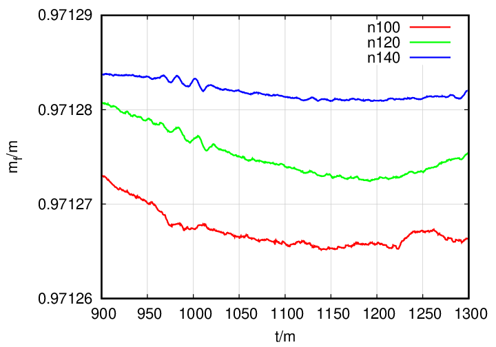
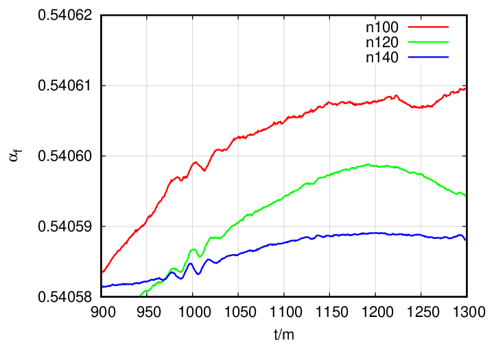
The final mass and final spin are measured very accurately by the horizon quasilocal formulas Dreyer et al. (2003a); Campanelli et al. (2007c); figs. 1 provide a visualization of their respective values after merger into the final settling black hole remnant. They display smaller variations versus time with increasing resolutions.

Figure 1: The horizon measure of the mass and spin after merger of a $q=1/3$ nonspinning binary versus time for $m\eta=2$ at resolutions n100, n120, n140.

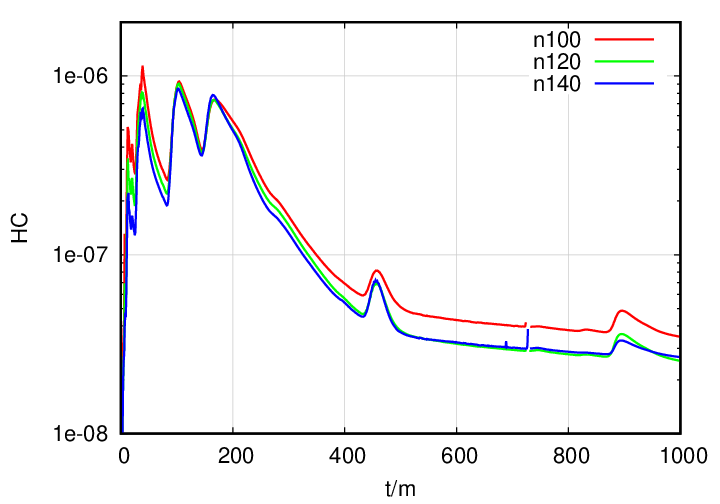
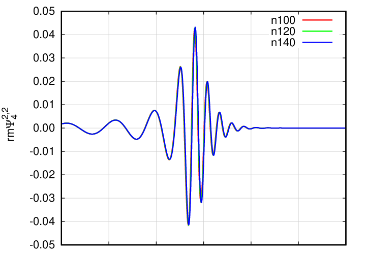
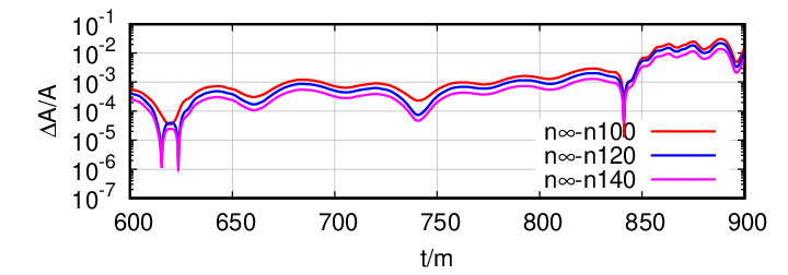
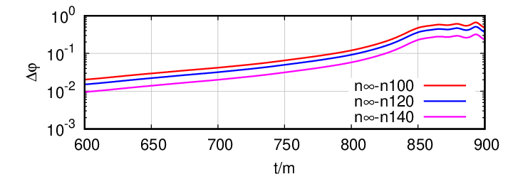
In Figs. 2 the convergence of the Hamiltonian constraint (Momentum constraints show a very similar convergent behavior) and the merger gravitational waveforms $(\ell,m)=(2,2)$-mode are displayed. Both show highly convergent behavior, therefore they are resolving the binary system accurately.

Figure 2: The Hamiltonian constraint behavior versus time for $m\eta=2$ at resolutions n100, n120, n140 in the top panel, and in the bottom panels, the (2,2)-waveform as seen by an observer at $R=113m$ for the $q=1/3$ nonspinning binary from an initial separation $D=9m$, the amplitude difference between resolutions, $\Delta A/A$, and the phase difference (in radians), $\Delta\varphi$, with respect to the infinite resolution extrapolation $(n_{\infty})$.

As shown in the Tables 1 and 2 the computed final mass and spin of the remnant black hole are well in the convergence regime at typical computation resolutions Healy et al. (2017b, 2019).

Table 1: The final black hole mass ($m_{f}/m$) for different $\eta$ and resolutions (top table). Difference between final black hole and ADM masses (bottom table). Values for $m\eta\to 0.0$ and resolution $h_{i}\to 0$ are extrapolated (the later by order $n$).

$h_{i}/m$	$m\eta=2.0$	$m\eta=1.0$	$m\eta=0.5$	$m\eta\to 0.0$
1/100	0.97127	0.97127	0.97128	0.97127
1/120	0.97128	0.97129	0.97126	0.97128
1/140	0.97128	0.97128	0.97128	0.97128
$\to 0$	0.97131	0.97135	0.97135	0.97132
$n$	1.59	2.24	1.95	2.29
1/100	0.02046	0.02046	0.02047	0.02046
1/120	0.02046	0.02045	0.02045	0.02044
1/140	0.02045	0.02045	0.02045	0.02045

Table 1 displays the difference between the initial total ADM mass and final horizon mass and Table 2 displays the loss of ADM angular momentum from its initial value to the final horizon spin for different resolutions and different ($\eta$-values) gauges. The computations give consistent values to 5-decimal places for each resolution, showing we are deep in the convergence regime and also versus $\eta$, showing (as expected) that those computations are gauge-invariant.

Table 2: The final black hole spin ($\alpha_{f}/m^{2}$) for different $\eta$ and resolutions (top table). Difference between final black hole angular momentum $\alpha_{f}$ and initial ADM angular momentum $J_{ADM}$ (bottom table). Values for $m\eta=0.0$ are extrapolated as those for infinite resolution $h_{i}\to 0$ with order $n$.

$h_{i}/m$	$m\eta=2.0$	$m\eta=1.0$	$m\eta=0.5$	$m\eta=0.0$
1/100	0.54060	0.54046	0.54060	0.54094
1/120	0.54059	0.54051	0.54060	0.54080
1/140	0.54059	0.54056	0.54059	0.54061
$\to 0$	0.54059	0.54110	0.54066	0.53857
$n$	1.58	0.85	2.24	0.93
1/100	-0.19185	-0.19187	-0.19183	-0.19186
1/120	-0.19184	-0.19185	-0.19184	-0.19185
1/140	-0.19183	-0.19184	-0.19184	-0.19184

To evaluate the convergence rate with three resolutions $h_{i}$ with $i=1,2,3$ we model the errors of a measured quantity $M_{i}=M(h_{i})$ as $A_{i}.h^{n}_{i}$ in such a way that the extrapolated to infinite resolution quantity $M_{\infty}=M(0)$ can be written as $M_{\infty}=M_{i}+\langle A\rangle h^{n}_{i}$, where $\langle A\rangle$ is an averaged value of the $A_{i}$. Thus for the three resolutions we have a system of three equations for the three unknowns, $M_{\infty}$, $n$, and $\langle A\rangle$. $n$ representing the convergence rate and $M_{\infty}$ the extrapolation to infinite resolution given in the tables below.

The corresponding computation of radiated energy and angular momentum from the waveforms extrapolated to an observer at infinity (from an extraction at $R=113m$) and summed over all $(\ell,m)$-modes up to $\ell=6$ are displayed in Tables 3 and 4 showing consistent approximate 3rd order convergence for the three resolutions n100, n120, and n140. When using the extrapolated to infinite resolution horizon values as exact, the convergence order increases, and is over 4th order for the radiated angular momentum. In all cases, the computations are consistent in the first 3 digits. While taking as the exact reference the extrapolated to infinite resolution horizon values, the convergence is over 4th order. Consistent first 4-digits are computed in all cases. Note that in all radiative computations we do not remove the initial data (spurious) radiation content to allow direct comparison with the corresponding horizon quantities.

Table 3: Energy radiated away in gravitational waves up to $\ell=6$ for the $q=1/3$ nonspinning binary. Values for $m\eta=0.0$ are extrapolated. Convergence order calculated from the three resolutions, $n$, and using the two highest resolutions and assuming the converged value is the value calculated on the horizon, $n(AH)$.

$h_{i}/m$	$m\eta=2.0$	$m\eta=1.0$	$m\eta=0.5$	$m\eta=0.0$
1/100	0.02017	0.02017	0.02017	0.02017
1/120	0.02030	0.02030	0.02029	0.02030
1/140	0.02036	0.02036	0.02036	0.02036
$\to 0$	0.02047	0.02045	0.02046	0.02046
$n$	3.03	3.23	3.08	3.10
$n(AH)$	3.31	3.23	3.18	—–

In particular, very weak dependence on $\eta$ is found, again as expected on the ground of gauge invariance of the gravitational waveform extrapolated to an observer at infinite location.

Table 4: Angular momentum radiated away in gravitational waves up to $\ell=6$ for the $q=1/3$ nonspinning binary. Values for $m\eta=0.0$ are extrapolated. Convergence order calculated from the three resolutions, $n$, and using the two highest resolutions and assuming the converged value is the value calculated on the horizon, $n(AH)$.

$h_{i}/m$	$m\eta=2.0$	$m\eta=1.0$	$m\eta=0.5$	$m\eta=0.0$
1/100	-0.19075	-0.19073	-0.19070	-0.19076
1/120	-0.19128	-0.19130	-0.19125	-0.19128
1/140	-0.19157	-0.19157	-0.19154	-0.19157
$\to 0$	-0.19217	-0.19196	-0.19215	-0.19216
$n$	2.56	3.38	2.62	2.55
$n(AH)$	4.78	4.50	4.62	—–

Tables 3 and 4 also show that both radiative quantities, energy and angular momentum show very small variations with respect to the extrapolated $\eta\to 0$ values, as expected from gauge invariant quantities.

Since the formula (5) is not gauge invariant when applied to the horizon of the final black hole we expect to find stronger variation with $\eta$ when we use it to evaluate the linear momentum of the remnant. We will pursue this exploration in more detail next in order to assess what values of $\eta$ allow us to compute the recoil velocity of the final black hole with a good accuracy. We are interested in particular, for our typical numerical simulations resolutions, what values of $\eta$ can produce more accurate values of the recoil from the horizon by use of (5) than from the evaluation of the radiated linear momentum at infinity.

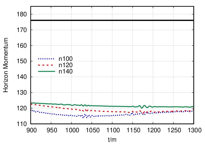
Our starting point is the gauge choices that we have been using regularly in our systematic studies of binary black hole mergers ($m\eta=2$ and Eqs. (2)) and numerical resolutions labeled by the resolution at the extraction level of radiation as n100, n120, n140, corresponding to wavezone resolutions of $h=1/1.00m,1/1.20m,1/1.40m$, respectively Healy et al. (2017b, 2019). We use 10 levels of refinement with an outer boundary at 400m. For each of these three resolutions we add a set of simulations by decreasing $\eta$ by factor of two, i.e. $\eta=1/m,1/2m$. The results of those nine simulations are displayed in Fig. 3. For $\eta=2/m$, the curves are very flat versus time after the merger with the highest resolution run, n140, being notably so. However their values for the evaluation of the recoil fall short compared to the estimate coming from the extrapolation of the radiative linear momentum to infinite resolution, represented by the solid black lines at about 177km/s.

Figure 3: The horizon measure of the linear momentum (in km/s) after merger of a $q=1/3$ nonspinning binary for the three resolutions n100 (dotted), n120 (dashed), and n140 (solid) for $\eta=2/m$ (blue), $1/m$ (red), $0.5/m$ (green). The reference value of $V_{f}$ (black solid line) is found by extrapolation to infinite resolution of the radiated linear momentum.

The progression towards smaller $\eta$ shows closer agreement with that extrapolated value. The time dependence shows variations as we approach the smaller $\eta$ but still converging with resolution towards the expected 177km/s value and flatter for n140, but clearly the limit $\eta\to 0$ requires much higher resolutions, as shown in Fig. 4. In our regime, reaching $\eta=1/m$ or $\eta=0.5/m$ seems a good compromise of accuracy versus cost of the simulation.

Figure 4: The horizon measure of the linear momentum (in km/s) after merger of a $q=1/3$ nonspinning binary lowering values of $\eta=2\to 0$ at resolution n140. The reference value of $V_{f}$ (black solid line) is found by extrapolation to infinite resolution of the radiated linear momentum.

Fig. 4 shows the progression of $m\eta=2.0,1.5,1.0,0.5,0.25$ for simulations with resolution n140. Notably they lie in a roughly linear convergence towards the expected higher recoil velocity value 177km/s, but as we reach the smaller $m\eta=0.25$ value it overshoots slightly, an effect of the required higher resolution needed to resolve accurately smaller values of $\eta$. In what follows we will restrict ourselves to values of $m\eta=2.0,1.0,0.5$ to make sure we are in a convergence regime for our standard resolutions n100, n120, n140. Note that we have verified that the simulation with n140 and $\eta=0$ does not crash, but leads to inaccurate results.

The radiation of linear momentum in terms of the Weyl scalar $\psi_{4}$, as given by the formulas in Campanelli and Lousto (1999b), can be computed in a similar fashion as we compute the energy and angular momentum radiated. For this study, we do not remove the initial burst of spurious radiation from the linear momentum calculation since we are interested in comparing to the final velocity of the merged BH. The burst will impart a (usually) small kick to the center of mass of the system. This allows direct comparison with horizon quantities in this paper. For astrophysical applications the removal of the initial burst of radiation is done in the waveform time domain and can be applied to remove their contributions to the final mass, spin and recoil velocity.

Table 5 shows that the radiation of linear momentum converges with resolution (at an approximate 2.6-2.7th order) at similar rates than the radiated energy and momentum (roughly 3rd order), and still varies little with $\eta$. This is expected on gauge invariance grounds.

Table 5: Total linear momentum radiated in gravitational waves up to $\ell=6$ for the $q=1/3$ nonspinning binary in km/s. Values for $m\eta=0.0$ are extrapolated. Convergence order $n$ is extrapolated to infinite resolution $h_{i}\to 0$. Bottom panel shows the angle (in degrees) of the net momentum with respect to the initial x-axis.

$h_{i}/m$	$m\eta=2.0$	$m\eta=1.0$	$m\eta=0.5$	$m\eta=0.0$
1/100	163.648	163.753	163.759	163.760
1/120	168.569	168.678	168.660	168.662
1/140	171.256	171.314	171.324	171.326
$\to 0$	176.750	176.422	176.708	176.702
$n$	2.582	2.699	2.608	2.611
1/100	375.01°	374.67°	373.61°	—–
1/120	374.93°	375.09°	374.54°	—–
1/140	375.50°	375.59°	375.78°	—–
$\to 0$	375.15°	375.12°	—–	—–
$n$	1.99	2.00	—–	—–

The values extrapolated to infinite resolution lie in the 176-177km/s range, consistently for all three values of $m\eta=2,1,0.5$. Extrapolations of the recoil velocities to $\eta\to 0$ are very close to their values at $m\eta=2,1,0.5$ for all three resolutions, again confirming the gauge independence of the results. In addition we display the angle (in degrees, reversed sign) the net radiated momentum has with respect to the x-axis (line joining the black hole initially).

Table 6: Horizon linear momentum measured at the interval $t=950m-1250m$ for the $q=1/3$ nonspinning binary in km/s. The bottom panel gives the angle (in degrees) this magnitude subtends with the initial x-axis. The measured standard deviation is given by the $\pm$ in the relevant quantities. Convergence order and extrapolations are given for $h_{i}\to 0$ and $\eta\to 0$.

$h_{i}/m$	$m\eta=2.0$	$m\eta=1.0$	$m\eta=0.5$	$m\eta=0.0$	order
1/100	$137.515\pm 1.12$	$160.507\pm 1.14$	$171.977\pm 3.99$	$183.397$	1.00
1/120	$139.543\pm 0.86$	$161.615\pm 1.36$	$174.703\pm 2.80$	$193.765$	0.75
1/140	$139.194\pm 0.40$	$165.014\pm 1.55$	$174.948\pm 0.87$	$181.161$	1.38
1/100	$373.83\degree\pm 0.27\degree$	$370.26\degree\pm 0.29\degree$	$367.52\degree\pm 0.86\degree$	358.475°	0.38
1/120	$373.87\degree\pm 0.48\degree$	$371.83\degree\pm 0.27\degree$	$373.64\degree\pm 0.36\degree$	372.909°	25.41
1/140	$374.63\degree\pm 0.58\degree$	$371.98\degree\pm 0.09\degree$	$374.37\degree\pm 0.16\degree$	373.389°	27.46
$\to 0$	374.11°	372.36°	375.81°	373.418°
$n$	2.00	6.07	6.11	18.53

Table 6 displays the crucial result of recoil velocities very close to their desired values for low resolutions when $m\eta=0.5$. They do not vary so much with resolution, as expected for horizon quantities, when compared to the variations with respect to the gauge choices. We observe close to a linear dependence on $\eta$ of the recoil values. Their extrapolation to $\eta\to 0$ overshoots the expected value by a few percent, but the values at $m\eta=0.5$ are nearly within 1%. This provides an effective way to compute recoils, since the corresponding radiative quantities are 3% away for n140. The horizon evaluations lying closer to the expected values by a factor 3 over the radiative ones holds for all three resolutions. In addition we display the angle the recoil velocity subtends with respect to the x-axis (line joining the black holes initially) showing a notable agreement of this sensitive quantity with the results in Table 5.

The coordinate velocities do not benefit systematically from the small $\eta$ gauges, but still provide a good bulk value as shown in Table 7. This shows the benefits of having a quasilocal measure of the momentum of the hole over its horizon compared to the local coordinate velocity of the puncture.

Table 7: Coordinate trajectory velocity in km/s as measured at $575m$ after merger for the $q=1/3$ nonspinning binary.

$h_{i}/m$	$m\eta=2.0$	$m\eta=1.0$	$m\eta=0.5$	$m\eta=0.0$
1/100	154.448	158.513	184.809	153.705
1/120	155.051	167.205	159.472	162.479
1/140	158.123	165.702	165.957	165.966

II.2 Validation for other mass ratios $(q=1/2,\ 1/5)$

In order to first validate our technique to extract the recoil velocity of the remnant black hole from spinning binaries, we have considered another unequal mass $(q=1/2)$ binary with initial separation $D=11m$. The resulting recoil will be along the orbital plane and due entirely to the asymmetry produced by the unequal masses. The results are presented in Table 8. Assuming the extrapolation to infinite resolution of the radiative linear momentum computations is the most accurate one leads to a recoil of $154.3\pm 0.1$km/s. Even for the lowest computed resolution, n100, the horizon evaluation for $m\eta=0.5$ at $159.6$km/s is a better approximation to that value than any radiative evolution at the same resolution (145.9km/s), with errors of the order of $3\%$. This is also true for the other two resolutions n120, and n140. Although, as we have seen before, the improvement of those horizon values are obtained by lowering the value of $m\eta\to 0$, rather than by higher resolution, as the horizon quasilocal measure has essentially already converged at those resolutions.

Table 8: Comparison of the computation of the recoil velocity (in km/s) of the remnant of a $q=1/2$, nonspinning binary by traditional radiation of linear momentum and the horizon formula (5) averaged between $t=1550m$ and $t=1850m$ for the traditional $\eta=2$ and for the $\eta=0.5$ case. Extrapolation to infinite resolution and convergence order is also given for the horizon and radiative extraction. The bottom panel gives the angle (in degrees) of the recoil velocity with respect to the x-axis. Standard deviations of horizon measurements are given as $\pm$ for each quantity. Convergence with numerical resolution is also given.

	Radiation	Horizon	Radiation	Horizon
$h_{i}/m$	$m\eta=2.0$	$m\eta=2.0$	$m\eta=0.5$	$m\eta=0.5$
1/100	145.45	$127.80\pm 0.65$	145.91	$159.57\pm 1.05$
1/120	149.45	$121.02\pm 0.79$	149.64	$152.48\pm 0.31$
1/140	151.38	$118.77\pm 0.65$	151.48	$152.92\pm 0.41$
$\to 0$	154.28	117.08	154.39	150.98
$n$	3.31	5.49	3.18	6.20
1/100	384.43°	$379.73\degree\pm 1.35\degree$	390.60°	$388.57\degree\pm 0.55\degree$
1/120	392.74°	$387.84\degree\pm 1.48\degree$	391.04°	$388.75\degree\pm 0.24\degree$
1/140	392.54°	$388.54\degree\pm 1.41\degree$	391.74°	$389.80\degree\pm 0.11\degree$
$\to 0$	394.75°	390.48°	—-	—–
$n$	6.17	6.14	—–	—–

Here we also provide the computation of the horizon evaluations for the mass and spin of the remnant black hole in Table 9. Those tables display the excellent agreement between the horizon and radiative computation of the energy and angular momentum (with convergence rates of the 3-4th order). It also displays the agreement of those radiative computations for the $\eta=2$ and the $\eta=0.5$ cases, as expected on the ground of gauge invariance at the extrapolated infinite observer location. The table also shows the robustness of the horizon computations at any of the used resolutions (generally 5 digits) and an overconvergence due to those small differences.

Table 9: Comparison of the computation of the horizon mass and spin of the remnant of a $q=1/2$, nonspinning binary with the radiation of the energy and angular momentum for the $\eta=2$ and for the $\eta=0.5$ cases. Extrapolation to infinite resolution and convergence order is also given for the horizon computation and the radiative extraction.

$m\eta=2.0$
$h_{i}/m$	$E_{rad}/m$	$J_{rad}/m^{2}$	$m_{f}/m$	$\alpha_{f}/m^{2}$	$\Delta m/m$	$-\Delta J/m^{2}$
1/100	0.02999	-0.30497	0.96126	0.62344	0.03029	-0.30617
1/120	0.03016	-0.30600	0.96125	0.62345	0.03030	-0.30617
1/140	0.03024	-0.30629	0.96125	0.62346	0.03030	-0.30617
$\to 0$	0.030337	-0.30646	0.96125	0.62346
$n$	3.70	6.36	13.36	6.09
$m\eta=0.5$
1/100	0.02998	-0.30516	0.96124	0.62343	0.03031	-0.30620
1/120	0.03014	-0.30583	0.96125	0.62345	0.03030	-0.30617
1/140	0.03022	-0.30615	0.96126	0.62345	0.03030	-0.30617
$\to 0$	0.03033	-0.30662	0.96126	0.62345
$n$	3.42	3.39	7.20	8.62

Table 10: Comparison of the computation of the horizon mass and spin of the remnant of a $q=1/5$, nonspinning binary with the radiation of the energy and angular momentum for the $\eta=2$ and for the $\eta=0.5$ cases. Extrapolation to infinite resolution $h_{i}\to 0$ and convergence order $n$ is also given for the horizon computation and the radiative extraction.

$m\eta=2.0$
$h_{i}/m$	$E_{rad}/m$	$J_{rad}/m^{2}$	$m_{f}/m$	$\alpha_{f}/m^{2}$	$\Delta m/m$	$-\Delta J/m^{2}$
1/100	0.01237	-0.15454	0.98217	0.41667	0.01253	-0.14804
1/120	0.01225	-0.14872	0.98235	0.41667	0.01235	-0.14790
1/140	0.01226	-0.14803	0.98237	0.41660	0.01232	-0.14796
$\to 0$	0.01227	-0.14788	0.98238	0.41667
$n$	11.59	11.41	10.78	-15.49
$m\eta=0.5$
1/100	0.01310	-0.16762	0.98158	0.41572	0.01320	-0.14944
1/120	0.01241	-0.15479	0.98221	0.41670	0.01249	-0.14800
1/140	0.01227	-0.14859	0.98236	0.41663	0.01234	-0.14795
$\to 0$	0.01221	-0.13922	0.98242	0.41662
$n$	8.12	3.30	7.59	14.39

We complete our nonspinning studies by simulating a smaller mass ratio $(q=1/5)$ binary with initial separation $D=10.75m$. The recoil from radiation of linear momentum extrapolates to about 139km/s as shown in Table 11. The horizon evaluation for $m\eta=2$ underevaluates this by about 30%, while for $m\eta=2$ the horizon formula is about 5% this value for the medium and high resolution runs. Given the smaller mass ratio, the low resolution run is not as accurate.

We also provide as a reference the computation of the of the horizon evaluations for the mass and spin of the remnant black hole in Table 10. Those tables display the excellent agreement between the horizon and radiative computation of the energy and angular momentum (with high convergence orders). We find excellent agreement of those radiative computations for the $\eta=2$ and the $\eta=0.5$ cases, as expected from the gauge invariance of the waveforms extrapolated to an infinite observer location. The table also shows the robustness of the horizon computations at medium and high resolutions (generally 3 digits) and an overconvergence due to those small differences.

Table 11: Comparison of the computation of the recoil velocity (in km/s) of the remnant of a $q=1/5$, nonspinning binary by traditional radiation of linear momentum and the horizon formula (5) averaged between $t=2300m$ and $t=2500m$ for the traditional $\eta=2$ and for the $\eta=0.5$ case. Extrapolation to infinite resolution $h_{i}\to 0$ and convergence order $n$ is also given for the horizon and radiative extraction. The bottom panel gives the angle (in degrees) of the recoil velocity with respect to the x-axis. Standard deviations of horizon measurements are given as $\pm$ for each quantity.

	Radiation	Horizon	Radiation	Horizon
$h_{i}/m$	$m\eta=2.0$	$m\eta=2.0$	$m\eta=0.5$	$m\eta=0.5$
1/100	129.40	$98.67\pm 0.60$	130.21	$209.00\pm 2.16$
1/120	133.91	$102.53\pm 0.16$	133.19	$131.93\pm 1.22$
1/140	135.94	$101.62\pm 0.13$	136.70	$143.28\pm 0.17$
$\to 0$	138.57	101.20	-	146.78
$n$	3.72	7.46	-	10.16
1/100	318.79°	$317.09\degree\pm 0.91\degree$	333.20°	$366.32\degree\pm 0.56\degree$
1/120	374.99°	$376.95\degree\pm 0.33\degree$	345.29°	$293.68\degree\pm 0.04\degree$
1/140	332.13°	$329.04\degree\pm 0.33\degree$	385.40°	$384.90\degree\pm 0.11\degree$

Table 12: Comparison of the computation of the recoil velocity (in km/s) of the remnant of a $q=1$, $\alpha_{i}=\pm 0.8$ binary by traditional radiation of linear momentum and the horizon formula (5) averaged between $t=1050m$ and $t=1350m$ for the traditional $\eta=2$ and the $\eta=1\text{ and }0.5$ cases. Extrapolation to infinite resolution $h_{i}\to 0$ and convergence order $n$ is also given for the radiative extraction. The bottom panel gives the angle (in degrees) of the recoil velocity with respect to the x-axis. Standard deviations of horizon measurements are given as $\pm$ for each quantity. In this case $m\eta=1$ produces a better measure of recoil velocity than other choices of $m\eta$.

	Radiation	Horizon	Radiation	Horizon	Radiation	Horizon
$h_{i}/m$	$m\eta=2.0$	$m\eta=2.0$	$m\eta=1.0$	$m\eta=1.0$	$m\eta=0.5$	$m\eta=0.5$
1/100	387.92	$331.98\pm 1.50$	-	-	388.13	$419.89\pm 0.30$
1/120	394.16	$331.84\pm 1.41$	394.13	396.41$\pm$0.22	394.16	$421.02\pm 0.38$
1/140	397.43	$331.75\pm 1.49$	-	-	397.16	$419.67\pm 0.86$
$\to 0$	403.42	331.40	-	-	402.00	-
$n$	2.82	1.46	-	-	3.12	-
1/100	135.51°	$135.81\degree\pm 0.93\degree$	-	-	135.70°	$137.25\degree\pm 0.27\degree$
1/120	136.70°	$135.72\degree\pm 0.92\degree$	136.65°	135.51°$\pm$0.27°	136.72°	$136.65\degree\pm 0.14\degree$
1/140	137.39°	$135.80\degree\pm 0.94\degree$	-	-	137.15°	$136.61\degree\pm 0.13\degree$
$\to 0$	139.07°	135.78°	-	-	137.60°	136.83°
$n$	2.23	4.26	-	-	4.23	4.29

Table 13: Comparison of the computation of the horizon mass and spin of the remnant of a $q=1$, $\alpha_{i}=\pm 0.8$ binary with the radiation of the energy and angular momentum for the $\eta=2$ and for the $\eta=0.5$ cases. Extrapolation to infinite resolution $h_{i}\to 0$ and convergence order $n$ is also given for the radiative extraction.

$m\eta=2.0$
$h_{i}/m$	$E_{rad}/m$	$J_{rad}/m^{2}$	$m_{f}/m$	$\alpha_{f}/m^{2}$	$\Delta m/m$	$-\Delta J/m$
1/100	0.03872	-0.34232	0.95071	0.68413	0.03936	-0.34403
1/120	0.03898	-0.34320	0.95071	0.68413	0.03936	-0.34403
1/140	0.03911	-0.34362	0.95071	0.68413	0.03936	-0.34404
$\to 0$	0.03930	-0.34421	0.95071	0.68413	-	-
$n$	3.28	3.45	-	-	-	-
$m\eta=1.0$
1/120	0.038979	-0.34318	0.95071	0.68413	0.03936	0.34404
$m\eta=0.5$
1/100	0.03872	-0.34232	0.95071	0.68413	0.03935	-0.34405
1/120	0.03898	-0.34318	0.95071	0.68413	0.03936	-0.34403
1/140	0.03911	-0.34358	0.95071	0.68413	0.03935	-0.34404
$\to 0$	0.03930	-0.34411	0.95071	0.68413	-	-
$n$	3.30	3.58	-	-	-	-

II.3 Spinning black holes

In order to further verify our technique to extract the recoil velocity of the remnant black hole from spinning binaries, we have considered an equal mass $(q=1)$ binary with spins $(\alpha_{1,2}=\pm 0.8)$ antialigned with the orbital angular momentum. This system has an initial separation of $D=10m$. The resulting recoil will be along the orbital plane and due entirely to the asymmetry produced by the opposing spins. The results are presented in Table 12, showing that assuming the extrapolation to infinite resolution of the radiative linear momentum computations is the most accurate one, leading to a recoil of $403\pm 1$km/s, even for the lowest computed resolution, n100, the horizon evaluation for $m\eta=0.5$ at $420$km/s is as good to that value than any radiative evolution at the same resolution (388km/s), with errors of the order of $4\%$. As we have seen before, the improvement of those horizon values are obtained by lowering the value of $m\eta\to 0$, rather than by higher resolution, as the horizon quasilocal measure has essentially already converged at those resolutions.

For the sake of completeness, and to verify the accuracy of the horizon evaluations for the mass and spin of the remnant black hole, we provide their computation in Tables 13. Those tables display the excellent agreement between the horizon and radiative computation of the energy and angular momentum (with convergence rates of the 3-4th order). It also displays the agreement of those radiative computations for the $\eta=2$ and the $\eta=0.5$ cases, as expected on the ground of gauge invariance at the extrapolated infinite observer location. Further, the tables show the robustness of the horizon computations at any of the used resolutions (generally 5 digits).

A final note on the convergence studies carried out in this section is that we observe a good convergence rate of 3rd to 4th order for radiative quantities while for horizon quantities a more wider range of values, with sometimes overconvergence. This is due to the fact that the horizon evaluations (particularly for the mass and spin) lead to very accurate values and hence small differences between the three resolutions chosen for the simulations (n100, n120, and n140). In order to seek very significant differences between resolutions, factors larger than 1.2 should be chosen (although requiring much larger computational resources). Note that nevertheless we have been able to prove that horizon quantities can be evaluated very accurately at any of the resolutions quoted above.

III Other Gauges Studies

Table 14: Comparison of the computation of the recoil velocity (in km/s) of the remnant of a $q=1/3$, $\alpha_{i}=\pm 0$ binary by traditional radiation of linear momentum and the horizon formula (5) measured $75m$ after merger. Computation uses the $\partial_{0}$-gauge $\eta=2$ case for resolutions n100 n120 and n140 and $\partial_{0}$-gauge $\eta=1,0.5$ cases for resolution n140. Extrapolation to infinite resolution $h_{i}\to 0$ and convergence order $n$ is also given for the radiative extraction for appropriate cases. The bottom panel gives the angle (in degrees) of the recoil velocity with respect to the x-axis. Standard deviations of horizon measurements are given as $\pm$ for each quantity. Compare this results with those of Tables 5-6.

	Radiation	Horizon	Radiation	Horizon	Radiation	Horizon
$h_{i}/m$	$m\eta=2.0$	$m\eta=2.0$	$m\eta=1.0$	$m\eta=1.0$	$m\eta=0.5$	$m\eta=0.5$
1/100	163.67	$127.11\pm 0.87$	—–	—–	—–	—–
1/120	168.57	$129.10\pm 0.98$	—–	—–	—–	—–
1/140	171.24	$128.84\pm 0.57$	171.30	$152.11\pm 1.92$	171.33	$160.9\pm 1.55$
$\to 0$	176.65	129.43	—–	—–	—–	—–
$n$	2.60	6.12	—–	—–	—–	—–
1/100	375.82°	$369.58\degree\pm 0.29\degree$	—–	—–	—–	—–
1/120	375.17°	$368.99\degree\pm 0.53\degree$	—–	—–	—–	—–
1/140	375.63°	$369.14\degree\pm 0.63\degree$	375.67°	$371.55\degree\pm 0.09\degree$	375.88°	$373.93\degree\pm 0.10\degree$
$\to 0$	—–	369.24°	—–	—–	—–	—–
$n$	—–	4.14	—–	—–	—–	—–

Right after the breakthrough that allowed evolving binary black holes with the moving puncture formalism Campanelli et al. (2006); Baker et al. (2006), several papers analyzed extensions of the basic gauges (2) - (4). In Refs. Gundlach and Martin-Garcia (2006) and van Meter et al. (2006) several parametrizations of the shift conditions are studied, and displayed some (slight) preference for the $\partial_{0}$-gauge over the $\partial_{t}$-gauge (See Table I of Ref. Gundlach and Martin-Garcia (2006) and Fig. 10 of Ref. van Meter et al. (2006)).

The sensitivity of the computed recoil on the gauge give us an opportunity to quantify the relative accuracy of the $\partial_{0}$-gauge versus the $\partial_{t}$-gauge.

We will also exploit the possibility of using a variable $\eta(x^{k}(t))$ to obtain both, the benefits of accuracy around the black holes and a good coordinate behavior connecting the horizon results with asymptotia.

III.1 $\partial_{0}$-gauge

Table 15: Top panel shows the comparison of the computation of the recoil velocity (in km/s) of the remnant of a $q=1$, $\alpha_{i}=\pm 0.80$ binary by traditional radiation of linear momentum and the horizon formula (5) averaged from $t/m=1050$ to 1350 using the $\partial_{0}$-gauge with $\eta=2$ and $\eta=0.5$ case at resolutions n100 and n120. The bottom panel gives the angle (in degrees) of the recoil velocity with respect to the x-axis. Both panels give also the $\partial_{t}$ results from Table 12 for comparison. Standard deviations of horizon measurements are given as $\pm$ for each quantity.

	Gauge	Radiation	Horizon	Radiation	Horizon
$h_{i}/m$	$\partial_{0},\partial_{t}$	$m\eta=2.0$	$m\eta=2.0$	$m\eta=0.5$	$m\eta=0.5$
1/100	$\partial_{0}$	387.94	$294.93\pm 2.43$	388.01	$377.37\pm 1.56$
1/100	$\partial_{t}$	387.92	$331.98\pm 1.50$	388.13	$419.89\pm 0.30$
1/120	$\partial_{0}$	394.18	$294.82\pm 2.41$	394.13	$376.89\pm 0.94$
1/120	$\partial_{t}$	394.16	$331.84\pm 1.41$	394.16	$421.02\pm 0.38$
1/100	$\partial_{0}$	135.53°	$135.71\degree\pm 1.00\degree$	135.78°	$137.31\degree\pm 0.27\degree$
1/100	$\partial_{t}$	135.51°	$135.81\degree\pm 0.93\degree$	135.70°	$137.25\degree\pm 0.27\degree$
1/120	$\partial_{0}$	136.71°	$135.62\degree\pm 1.00\degree$	136.69°	$136.65\degree\pm 0.18\degree$
1/120	$\partial_{t}$	136.70°	$135.72\degree\pm 0.92\degree$	136.72°	$136.65\degree\pm 0.14\degree$

In Fig. 5 we draw a comparative analysis of the final black hole horizon recoil as computed in the $\partial_{0}$ and $\partial_{t}$ gauges, at our highest resolution n140. In all three cases, $\eta=2,1,0.5$, the computation in the $\partial_{t}$-gauge is notably and systematically closer to the expected ($V_{f}\sim 177$km/s) recoil velocity. This also provides a scale of the accuracy of the evaluation of the recoil for our new preferred value, $\eta=0.5$.

Figure 5: Comparative results of the $\partial_{t}$-gauge (solid) and $\partial_{0}$-gauge (dashed) for the horizon measure of the linear momentum (in km/s) after merger of a $q=1/3$ nonspinning binary for the n140 resolution for $\eta=2/m$ (blue), $1/m$ (green), $0.5/m$ (red). The reference value of $V_{f}$ is found by extrapolation to infinite resolution of the radiated linear momentum.

Convergence with resolution does not resolve this discrepancies in favor of the $\partial_{t}$-gauge as displayed in Fig. 6 for $m\eta=2$ in in the $\partial_{0}$-gauge at n100, n120, and n140 resolutions. With the limit $\eta\to 0$ being even harder to resolve than in the $\partial_{t}$-gauge case.

Figure 6: The horizon measure of the linear momentum (in km/s) after merger of a $q=1/3$ nonspinning binary for the three resolutions labeled as n100, n120, and n140 in the $\partial_{0}$-gauge for $\eta=2/m$. The reference value of $V_{f}$ is found by extrapolation to infinite resolution of the radiated linear momentum in this $\partial_{0}$-gauge.

Those results for the evolutions in the $\partial_{0}$-gauge are summarized in Table 14 were we should compare its results with those in Tables 4-5 in the $\partial_{t}$-gauge. While the computation of the extracted radiation are comparable and convergent to essentially the same values, i.e. a recoil magnitude of about 177km/s and an angle with the $x$-axis of $375\degree$, the closeness to those values in the $\partial_{t}$-gauge is apparent for all values of $\eta$. A second control case is studied in Table 15, were we consider the spinning binary system described in Section II.3. We directly compare the $\partial_{0}$-gauge new simulations with the $\partial_{t}$-gauge simulations reported in Table 12. Based on those results we expect recoil magnitudes in the 402-403km/s and angles in the $138\degree-139\degree$ ranges. The results for $\eta=2$ confirms the closer to the expected recoils in the $\partial_{t}$-gauge, and those of $\eta=0.5$ bracket it, with preference for the $\partial_{t}$-gauge. We also observe again that the horizon values are much more sensitive to the values of $\eta$ than to resolutions (at least for these 1.2 increase factors).

In conclusion we observe the advantage of working in the $\partial_{t}$-gauge over the $\partial_{0}$-gauge regarding computation of recoil velocities from the horizon formula (5). This agrees with our generic experience for binary black holes simulations being more accurate in our standard $\partial_{t}$-gauge at the same resolutions and same values of $\eta$, but now we have quantified it in the recoil computations example. As we converge to higher resolutions, both gauges lead to consistent and accurate solution in all studied quantities.

III.2 $\eta$-variable gauge

Table 16: Comparison of the computation of the recoil velocity (in km/s) of the remnant of a $q=1/3$, $\alpha_{i}=0$ binary by traditional radiation of linear momentum and the horizon formula (5) measured $75m$ after merger for the modified N12 and N10 gauges. The standard $\eta=1$ from Tables 5 and 6 is also provided for reference. Extrapolation to infinite resolution $h_{i}\to 0$ and convergence order $n$ is also given for the radiative extraction. The bottom panel gives the angle (in degrees) of the recoil velocity with respect to the x-axis. Standard deviations of horizon measurements are given as $\pm$ for each quantity.

	Radiation	Horizon	Radiation	Horizon	Radiation	Horizon
$h_{i}/m$	N12	N12	N10	N10	$m\eta=1$	$m\eta=1$
1/100	163.65	$169.88\pm 1.29$	163.71	$150.54\pm 1.18$	163.75	160.51$\pm$1.14
1/120	168.59	$172.56\pm 0.75$	168.61	$153.52\pm 0.86$	168.66	161.62$\pm$1.36
1/140	171.20	$177.64\pm 1.78$	171.26	$155.31\pm 1.75$	171.31	165.01$\pm$1.55
$\to 0$	176.09	—–	176.52	160.14	176.42	—–
$n$	2.78	—–	2.64	2.04	2.70	—–
1/100	373.01°	$371.21\degree\pm 0.93\degree$	374.39°	$364.97\degree\pm 0.27\degree$	374.67°	370.26°$\pm$0.29°
1/120	374.02°	$373.17\degree\pm 0.92\degree$	374.85°	$366.81\degree\pm 0.14\degree$	375.09°	371.83°$\pm$0.27°
1/140	374.72°	$377.24\degree\pm 0.94\degree$	375.57°	$367.90\degree\pm 0.13\degree$	375.59°	371.98°$\pm$0.09°
$\to 0$	378.40°	377.24°	—–	—–	375.12°	372.36°
$n$	1.13	2.15	—–	—–	2.00	6.07

Table 17: Comparison of the computation of the recoil velocity (in km/s) of the remnant of a $q=1$, $\alpha_{i}=\pm 0.80$ binary by traditional radiation of linear momentum and the horizon formula (5) measured from $t/m=1050\text{ to }1350$ for the modified N12 and N10 gauges using $\eta\to 1$ asymptotically, as well as $m\eta=1.0$ for comparison. The bottom panel gives the angle (in degrees) of the recoil velocity with respect to the x-axis. Standard deviations of horizon measurements are given as $\pm$ for each horizon quantity.

	Radiation	Horizon	Radiation	Horizon	Radiation	Horizon
$h_{i}/m$	N12	N12	N10	N10	$m\eta=1.0$	$m\eta=1.0$
1/120	394.88	$379.66\pm 0.80$	393.87	$335.74\pm 1.10$	394.13	396.41$\pm$0.22
1/120	137.44°	$141.54\degree\pm 0.46\degree$	136.38°	$128.90\degree\pm 0.08\degree$	136.65°	135.51°$\pm$0.27°

In addition to the changes in the (constant) values of $\eta$, different functional dependences for $\eta(x^{k},t)$ have been proposed in Zlochower et al. (2005); Müller and Brügmann (2010); Müller et al. (2010a); Schnetter (2010); Alic et al. (2010); Lousto and Zlochower (2011).

Here we use a modified form motivated by the results of Krishnan et al. (2007) and this paper that the recoil velocities (of a merged binary) are more accurately computed when using the quasilocal horizon measure of the momentum with smaller $\eta$ and that the generic evolution is more accurate and convergent for larger values of $\eta$.

We hence propose a simple variant for comparable masses binary

$$m\eta(x^{k},t)=m\eta_{\infty}-A\,e^{-r^{2}/s^{2}}$$ (6)

where $m=m_{1}+m_{2}$ and $r=|\vec{r}-\vec{r}_{com}|$ is the distance from the (Newtonian) center of mass of the system [PN corrections could be added if needed Bernard et al. (2018)],

$$\vec{r}_{com}=(m_{1}\,\vec{x}_{1}+m_{2}\,\vec{x}_{2})/m$$ (7)

where $\vec{x}_{1}(t)$ and $\vec{x}_{2}(t)$ are the punctures location, and $s$ is a width of the Gaussian that can be conveniently chosen, for instance, $s=2m$. Typically for our simulations normalization is chosen such that $m\sim 1$ (and $M_{ADM}<1$).

The choice to center the Gaussian correction to the $\eta_{\infty}$ at the center of mass is to provide a simple way of following the final black hole after merger, even if acquired a large recoil velocity. The motivation to set different values around the black hole is to provide enough accuracy and convergence in the strong field regime, while preserving the benefits of the coordinates adapted to recoil measurements away from the remnant hole.

In order to assess those statements we have considered two cases labeled as N10 and N12, respectively determined by the $-$ and $+$ in

$$m\eta(x^{k},t)=1\mp\,e^{-r^{2}/(2m)^{2}}$$ (8)

with the same reference asymptotic value of 1 at infinity and vanishing or taking the standard value of 2 at the (final) hole location.

The simulations (in the standard $\partial_{t}$-gauge) make use of this (8) dependence during the whole run, not only during the post-merger phase, but the horizon of the final black hole is only found and evaluated for linear momentum after the merger occurs (about $t\sim 725m$).

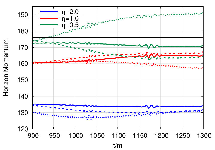
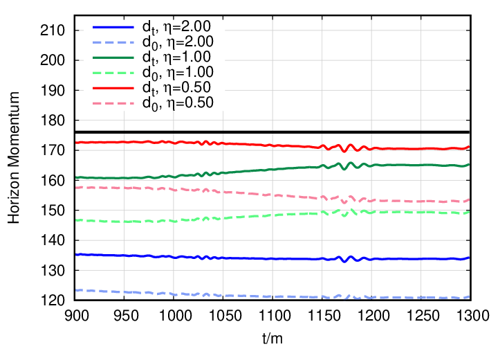
The results of the two cases are displayed in Fig. 7. Each case has been studied at our standard n100, n120, n140 resolutions to convey an idea of the convergence. The upper panel displays a very good agreement with the expected recoil, particularly for the medium and high resolutions. The agreement is even better than the constant $m\eta=1$ case, displayed in the central panel of Fig. 3, which lies in between the N12 and N10 cases. To confirm the improvements reached by this variable-$\eta$ gauge, the case N10, where the asymptotic value is the same, equal to 1, but where the $\eta$ is reduced near the black hole, reduces notably the accuracy necessary to compute the linear momentum of the horizon and convergence is still more challenging than in the previous N12 case.

Figure 7: The horizon measure of the linear momentum after merger of a $q=1/3$ nonspinning binary for the three resolutions labeled as n100 (dotted), n120 (dashed), and n140 (solid) for $\eta=$ N12 (red) and N10 (blue), top to bottom respectively. The reference value of $V_{f}$ is found by extrapolation to infinite resolution of the radiated linear momentum.

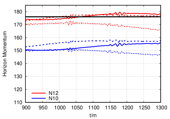
Those results for the variable $\eta$-gauge, as in (8) are summarized in Table 16 were we compare its results with those in Tables 4-5 in the $\eta=1$-gauge. While the computation of the extracted radiation are comparable and convergent to essentially the same values, i.e. a recoil magnitude of about 176-7km/s and an angle with the $x$-axis of 375-6°, the closeness to those values in the N12-gauge is apparent followed by the $m\eta=1$ (the reference value) and lagged by the N10-gauge, indicating that while the same asymptotic $m\eta=1$ value is shared by the three gauges, that with $m\eta\to 2$ near the horizon of the black hole produces the most accurate results for the recoil computed via the horizon formula (5).

A second control case is studied in Table 17, were we consider the spinning binary system described in Section II.3. We directly compare the N12-N10-gauge new simulations with each other using the radiation values as the more accurate references, and we find again the confirmation that the N12 results are much closer to the expected results than the N10 ones.

In conclusion, a first exploration of an $\eta$-variable leads to immediate benefits and opens the possibilities for further refinement of its parameters to have both, accuracy and precision improved in the numerical simulations of merging binary black holes.

III.3 Small mass ratio

Because of the technical similarities (although with complementary mass ratio applications), here we briefly discuss dealing with the small mass ratio binaries by the modeling of the damping parameter $\eta$. The proposal for $\eta$ in Eq. (6) is meant to be used for comparable masses $q>1/10$ when we can still use a constant $\eta$ for evolutions. For smaller mass ratios this $\eta_{\infty}$ can be replaced by the $\eta(W)$ (the conformal factor $W=\sqrt{\chi}=\exp(-2\phi)$ suggested by Marronetti et al. (2008)) used in Ref. Lousto and Zlochower (2011) or a modification of it given below or yet other based on superposition of weighted Gaussians. Note that the recoil for $q<1/10$ is small. This question has been already studied in Müller and Brügmann (2010); Lousto et al. (2010b); Müller et al. (2010b); Alic et al. (2010); Schnetter (2010)

Here we simply bring back some of those ideas, assuming we evaluate $\eta(\vec{r}_{1}(t),\vec{r}_{2}(t))$ parametrized by the black holes 1 and 2 punctures trajectories $(\vec{r}_{1}(t),\vec{r}_{2}(t))$

The (initial) conformal factor evaluated at every time step is

$$\psi_{0}=1+{\frac{m_{1}}{{|\vec{r}-\vec{r}_{1}(t)|}}}+{\frac{m_{2}}{{|\vec{r}-\vec{r}_{2}(t)|}}}$$ (9)

And we can then define analogously to the $\eta(W)$

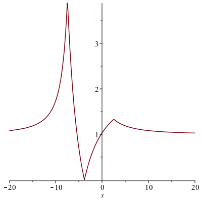
$$m\eta_{\psi}=A+B\,{\frac{\sqrt{|\vec{\nabla}_{r}\psi_{0}|^{2}}}{\left(1-{\psi_{0}}^{a}\right)^{b}}}.$$ (10)

We plot an example in Fig. 8. At the puncture $m\eta=2$ and at the center of mass $m\eta=2.04$, but it goes through a minimum $m\eta=0$ and a this point, as well as the punctures, $\eta$ is $C^{0}$. Since the gauge condition Eq. (2) involves an integration, this might still be fine for evolutions (as well as at the punctures).

Figure 8: $\eta_{\psi}$ profile for ($m=m_{1}+m_{2}=1$ here) $m_{1}=1/4$, $m_{2}=3/4$; $x_{1}=-7.5$, $x_{2}=2.5$; $a=1$, $b=2$; $A=1$, $B=1$.

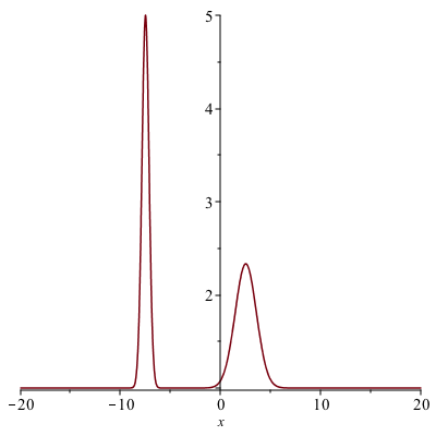
A second alternative smoother behavior is the superposition of Gaussian (See also Müller et al. (2010b))

$$\eta_{G}=\frac{A}{m}+{\frac{B}{m_{1}}{e^{-|\vec{r}-\vec{r}_{1}(t)|^{2}/{s_{1}}^{2}}}}+{\frac{C}{m_{2}}{e^{-|\vec{r}-\vec{r}_{2}(t)|^{2}/s_{2}^{2}}}},$$ (11)

which for the parameters of the previous example we display in Fig. 9, behaving like 1.25 at the first puncture, 1.75 at the second and is essentially 1 in between and far away from the binary.

Figure 9: $\eta_{G}$ profile for ($m=m_{1}+m_{2}=1$ here) $m_{1}=1/4$, $m_{2}=3/4$; $x_{1}=-7.5$, $x_{2}=2.5$; $A=1$, $B=1$, $C=1$; $s_{1}=2\,m_{1}$, $s_{2}=2\,m_{2}$

The explicit application and evaluations in actual simulations of small mass ratio binary black hole mergers is left for an independent study (Healy et al. 2020b, paper in preparation).

IV Discussion

The purpose of this study was to assess what choices of $\eta$ lead to accurate measures of the linear momentum of the horizon with the non-gauge-independent formula (5), and we found that for small values $m\eta\leq 0.5$ this is a reliable measure and can compete with the measurement at $\mathscr{I}^{+}$ of the radiated momentum carried by the gravitational waves. As with the computations of the mass and angular momentum of the remnant via the horizon measure and at infinity, it is important to have two concurrent methods to assess errors of those measures. Further accuracy could be achieved by the use of a variable $\eta$ (See Eq. (6). Our results indicate that the choice of $m\eta=2$ at the horizon, with lower values at asymptotically far distances from the source(s), produce the best results for evaluation of the recoil.

While these gauges were studied in detail for a nonspinning $q=1/3$ binary and verified as control cases for the $q=1/2$ and $q=1/5$ binaries as well as for a $q=1$ spinning case, we expect these conclusions to be general and plan to apply the findings to simulations where the computation of recoil is important, including precessing binaries. The cross checking with radiated linear momentum will provide a control to its applicability and can be carried out concurrently in each simulation.

Finally, we have been able to assess the relative accuracy of the two original moving puncture choices for the shift, the $\partial_{t}$ and $\partial_{0}$ gauges regarding their accuracy to evaluate the recoil and found that the $\partial_{t}$-gauge seems to be superior, at the current typical numerical resolutions.