Cosmological Bounds on sub-GeV Dark Vector Bosons
from Electromagnetic Energy Injection

John Coffey^(a), Lindsay Forestell^(b,c),
David E. Morrissey^(c), and Graham White^(c)

(a) Department of Physics and Astronomy, University of Victoria,
Victoria, BC V8P 5C2, Canada
(b) Department of Physics and Astronomy, University of British Columbia,
Vancouver, BC V6T 1Z1, Canada
(c) TRIUMF, 4004 Wesbrook Mall, Vancouver, BC V6T 2A3, Canada
email: jwcoffey@uvic.ca, lmforest@phas.ubc.ca,
dmorri@triumf.ca, gwhite@triumf.ca

New dark vector bosons that couple very feebly to regular matter can be created in the early universe and decay after the onset of big bang nucleosynthesis (BBN) or the formation of the cosmic microwave background (CMB) at recombination. The energy injected by such decays can alter the light element abundances or modify the power and frequency spectra of the CMB. In this work we study the constraints implied by these effects on a range of sub-GeV dark vectors including the kinetically mixed dark photon, and the $B\!-\!L$, $L_{e}\!-\!L_{\mu}$, $L_{e}\!-\!L_{\tau}$, and $L_{\mu}\!-\!L_{\tau}$ dark $U(1)$ bosons. We focus on the effects of electromagnetic energy injection, and we update previous investigations of dark photon and other dark vector decays by taking into account non-universality in the photon cascade spectrum relevant for BBN and the energy dependence of the ionization efficiency after recombination in our treatment of modifications to the CMB.

1 Introduction

Direct measurements of the cosmos give strong evidence for a standard $\Lambda\text{CDM}$ cosmology containing the elementary particles and forces predicted by the Standard Model (SM) [1, 2]. Observations of the cosmic microwave background (CMB) [3, 4], baryon acoustic oscillations (BAO) [5, 6, 7], and supernovae distances [8, 9, 10] fix the parameters of the $\Lambda\text{CDM}$ model very precisely. The success of big bang nucleosyntheis (BBN) at predicting the light element abundances (notwithstanding the lithium puzzles) provides further support for a $\Lambda\text{CDM}$ cosmology with SM particles and interactions going back even earlier in time, up to temperatures on the order of a few MeV [11, 12, 13, 14, 15, 16, 17, 18].

Tests of the SM+$\Lambda\text{CDM}$ paradigm also put stringent constraints on a broad range of new physics beyond the SM and deviations from the standard cosmology. In particular, processes that inject energy into the cosmological plasma can modify BBN by altering the ratio of neutrons to protons or destroying/creating light elements. These considerations have been used to constrain new (effective) light degrees of freedom [19, 20, 21, 22, 23, 24, 25, 26, 27, 28, 29, 30], the minimum temperature of reheating or periods of non-standard cosmological evolution [31, 32, 33], and the decays [34, 35, 36, 37, 38, 39, 40, 41, 42, 43, 44, 45, 46, 47] or annihilations [48, 49, 50, 51, 52] of particles in the early universe. Related bounds can be derived on late-time energy injection from the deviations induced in the CMB frequency [53, 54] and power spectra [55, 56, 57, 58, 59, 60, 61, 62].

In this work we apply and extend these methods to derive cosmological bounds from BBN and the CMB on a range of sub-GeV dark vector bosons. New vector bosons are ubiquitous in extensions of the SM, including grand unification [63, 64, 65], superstring theory [66, 67, 68], and theories of dark matter [69, 70, 71]. By definition, dark vector bosons couple only very feebly to the SM, and can thus be much lighter than the electroweak scale without having been discovered yet [72, 73, 74]. For very small couplings, dark vectors are very difficult to produce in the laboratory and can develop macroscopically long lifetimes. Thermal cosmological production is also reduced in this regime and the dark vectors might never develop a full thermal abundance. Even so, dark vector bosons can still be created in the early universe through direct reheating [75, 76, 77, 78], freeze-in processes [79, 80, 81, 82, 83], or the decays or annihilations of heavier dark states [84, 85]. The later decays of the vector bosons then inject energy into the cosmological medium, possibly modifying the light element abundances and the CMB relative to SM+$\Lambda\text{CDM}$ [86, 87].

We investigate a range of light (but massive) U(1) vector bosons including a dark photon (DP) that connects to the SM exclusively through gauge kinetic mixing with hypercharge [88, 89], as well as the anomaly-free combinations $B\!-\!L$ [90, 91], $L_{e}\!-\!L_{\mu}$ [92], $L_{e}\!-\!L_{\tau}$ [92], and $L_{\mu}\!-\!L_{\tau}$ [93, 94] with only very tiny direct couplings to the SM. Our focus is on the mass range $m_{V}\in[1\,\,{\rm MeV},\,1\,\,{\rm GeV}]$ over which these dark vectors have significant decay fractions to electromagnetic channels, and we concentrate on the impact of the electromagnetic component of the energy injected by the decays which is typically the most important effect for lifetimes greater than $\tau_{V}\gtrsim 10^{4}\,\mathrm{s}$.

This study expands on previous investigations of cosmological bounds on dark photons in two ways [86, 87]. First, applying the technology developed in Ref. [95], we compute the full electromagnetic cascade induced by dark vector decays, including some new effects relative to Refs. [86, 87]. From this we derive the resulting photon cascade spectrum that is essential for determining the impact of electromagnetic energy injection on the light element abundances. Our calculation also differs from the more common approach of using the universal photon spectrum defined in Ref.[42], based on the results of Refs. [39, 96, 97, 98, 99], to derive the cascade photon spectrum. The universal spectrum method provides a very good description of the photon cascade produced by the interactions of highly-energetic electromagnetic primaries ($E\gtrsim 100\,\,{\rm GeV}$) with the cosmological background prior to recombination, and has the major simplifying feature that it only depends on the total amount of electromagnetic energy injected rather than the detailed primary injection spectrum. However, it was shown in Refs. [95, 100, 101, 102] that lower-energy electromagnetic injection near or below the GeV scale can lead to cascade photon spectra that deviate significantly from the predictions of the universal spectrum, and that can depend on the type and spectrum of the energy [95].

In light of this first point, the second way that we expand on previous work is by computing the detailed primary electromagnetic injection spectra from sub-GeV vector boson decays [103, 104]. We study the energy spectra of electrons and photons created by the decay modes $V\to\{e^{+}e^{-},\,\mu^{+}\mu^{-},\,\pi^{+}\pi^{-},\,\pi^{+}\pi^{-}\pi^{0},\,\pi^{0}\gamma\}$, which are expected to be the most important ones for the dark vectors of interest [105, 106]. We then apply these injection spectra to computing the full electromagnetic cascade spectrum produced by a given dark vector decay for our BBN studies or use them to calculate limits from the CMB.

The outline of this paper is as follows. In Sec. 2 we compute the decay rates and fractions of the dark vector species and we find the energy spectra of the resulting photons and electrons. Next, in Sec. 3 we study the effects of electromagnetic energy injected by dark vector decays on the light elements and use current data to set limits on the pre-decay dark vector densities as a function of their lifetime and mass. We investigate the related effects of dark vector decays on the power and frequency spectra of the CMB in Sec. 4. In Sec. 5 we review the calculation of the density of dark vectors from thermal production in the early universe, and we find the constraints from BBN and the CMB on the masses and couplings of dark vectors for the corresponding thermal yields. Finally, Sec. 6 is reserved for our conclusions. Some additional details on the departure from electromagnetic universality in BBN and when it occurs are presented in Appendix A.

2 Dark Vector Bosons and their Decays

We begin by reviewing the dominant decay channels for the sub-GeV dark vector bosons of interest: kinetically mixed dark photon (DP), $B\!-\!L$, $L_{e}\!-\!L_{\mu}$, $L_{e}\!-\!L_{\tau}$, $L_{\mu}\!-\!L_{\tau}$. In all cases we assume the dark vectors decay exclusively to the SM, with no additional exotic decay channels available. With the decay fractions in hand, we turn next to computing the electron and photon spectra they produce in the rest frame of the dark vector relevant for computing cosmological bounds on them.

2.1 Vector Boson Decay Branching Fractions

The sub-GeV dark vectors under consideration interact with the SM primarily through gauge kinetic mixing for the dark photon (DP),

$$\mathscr{L}\ \supset\ -\frac{\epsilon}{2}\,F_{\mu\nu}V^{\mu\nu}$$ (1)

with kinetic mixing parameter $\epsilon$, and via direct gauge coupling to the SM for the rest,

$$\mathscr{L}\ \supset\ -g_{V}\bar{f}\gamma^{\mu}(Q_{L}P_{L}+Q_{R}P_{R})f\,V_{\mu}$$ (2)

where $g_{V}\ll 1$ and we normalize to $|Q_{L}|=1$ for leptons. The direct-coupling dark vectors will also have a gauge kinetic mixing with the photon but we assume (self-consistently) that it is sub-leading relative to the direct gauge interaction. We assume further that the dark vectors obtain a mass $m_{V}$ in the MeV–GeV range from the Higgs [107] or Stueckelberg [108, 109] mechanisms, and that no decay channels to light SM-singlet states are available. In particular, for the direct-coupling vectors we assume as in Ref. [106] that the light neutrinos are Majorana and mostly left-handed (which requires a spontaneous breaking of the underlying gauge invariance), and that any SM singlets are heavy enough to be neglected.

With these couplings, the perturbative decay widths to SM fermions $f$ are

$$\Gamma(V\to f\bar{f})=N_{c}\frac{\alpha_{V}}{6}\,m_{V}\,\sqrt{1-\left(\frac{2m_{f}}{m_{V}}\right)^{2}}\;\left(Q_{L}^{2}+Q_{R}^{2}+\left[6Q_{L}Q_{R}-(Q_{L}^{2}+Q_{R}^{2})\right]\frac{m_{f}^{2}}{m_{V}^{2}}\right)$$ (3)

where $N_{c}$ is the number of QCD colours of the fermion, $\alpha_{V}=\epsilon^{2}\alpha$ for the dark photon (with $Q_{L,R}=Q_{em}$), and $\alpha_{V}=g_{V}^{2}/4\pi$ for the direct vectors (with $Q_{R}=0$ for the light neutrinos given the assumptions stated above).

For sub-GeV vectors, we must also consider decays of the vector to specific hadronic states. Since these decays are strongly suppressed for the leptonic vectors, we only include them for the DP and $B\!-\!L$ vectors here. Our approach to describing hadronic dark vector decays uses a combination of the data-driven methods of Refs. [86, 105, 106] and the analytic description based on vector-meson-dominance (VMD) of Ref. [110]. In the VMD picture [111, 112, 113, 114], which also guides the methods of Refs. [86, 105, 106], the $\rho$ and $\omega$ vector mesons are treated as gauge bosons of a hidden $U(2)$ flavour symmetry. Dark vector decays to hadrons in this picture occur through direct couplings – the DP to the electromagnetic current and the $B\!-\!L$ vector to the baryonic current – as well as through an induced kinetic mixing with the $\rho$ and $\omega$ with approximate strength [110, 105]

$$\epsilon_{VMD}\ \simeq\ 2\,\text{tr}(t_{A}\,Q_{V})\,\frac{g_{V}}{g}\ =\ \frac{g_{V}}{g}\times\left\{\begin{array}[]{ccl}1&;&\text{DP -- }\rho\\ 1/3&;&\text{DP -- }\omega\\ 0&;&(B\!-\!L)\text{ -- }\rho\\ 2/3&;&(B\!-\!L)\text{ -- }\omega\end{array}\right.$$ (8)

where $t_{A}=\text{diag}\big{(}1/2,\,\pm 1/2\big{)}$ for $A=\omega,\,\rho$ is the $U(2)$ generator, $g\simeq\sqrt{3\times 4\pi}$, $Q_{V}=\text{diag}\big{(}2/3,\,-1/3\big{)}$ for DP and $Q_{V}=\text{diag}\big{(}1/3,\,1/3\big{)}$ for $B\!-\!L$, and $g_{V}=-e\epsilon$ for the DP.

The leading hadronic decay mode of the dark photon is usually $V\to\pi^{+}\pi^{-}$. In the VMD picture, it arises from a combination of the direct countribution of the charged pions to the electromagnetic current and the induced kinetic mixing with the $\rho$. The corresponding decay width is

$$\Gamma(\text{DP}\to\pi^{+}\pi^{-})\ =\ \frac{\alpha_{V}}{12\pi}\left[1-\left(\frac{2m_{\pi^{+}}}{m_{V}}\right)^{2}\right]^{3/2}|F_{\pi\pi}(m_{V})|^{2}\ ,$$ (9)

where the leading-order form factor is [114]

$$F_{\pi\pi}\ \simeq\ 1-\frac{g_{\rho\pi\pi}}{g}\frac{s}{s-m_{\rho}^{2}+im_{\rho}\Gamma_{\rho}(s)}\ ,$$ (10)

with $g_{\rho\pi\pi}\simeq g$, $m_{\rho}=775.25\,\,{\rm MeV}$, and $\Gamma_{\rho}(s=m_{\rho})=149\,\,{\rm MeV}$. The true form factor is modified relative to Eq. (10) by the energy dependence of the $\rho$ self-energy as well as $\rho$-$\omega$ mixing. In our analysis we follow Ref. [105] and extract the form factor from $e^{+}e^{-}\to\pi^{+}\pi^{-}(\gamma)$ measurements by the BABAR experiment [115]. Note that $\rho$-$\omega$ mixing also allows the $B\!-\!L$ vector to decay to $\pi^{+}\pi^{-}$ but we do not include the effect because the branching fraction for this channel is always less than a couple percent.

Mixing with the $\omega$ allows the DP and $B\!-\!L$ vectors to decay to $\pi^{+}\pi^{-}\pi^{0}$ and $\pi^{0}\gamma$, with the effect being strongest near the $\omega$ mass. The width for $V\to\pi^{0}\gamma$ is [110]

$$\Gamma(V\to\pi^{0}\gamma)\ =\ \Big{[}2\text{tr}(t_{A}Q_{V})\Big{]}^{2}\,\frac{3\,\alpha_{V}}{128\pi^{3}}\frac{m_{V}^{3}}{f_{\pi}^{2}}\,|F_{\omega}(m_{V}^{2})|^{2}\ .$$ (11)

For the decay $V\to\pi^{+}\pi^{-}\pi^{0}$, the width is [110]

$$\Gamma(V\to\pi^{+}\pi^{-}\pi^{0})\ =\ \Big{[}2\text{tr}(t_{A}Q_{V})\Big{]}^{2}\,\frac{3\,\alpha_{V}}{16\pi^{4}}\left(\frac{g^{2}}{4\pi}\right)^{\!2}\frac{m_{V}}{f_{\pi}^{2}}\,\mathcal{I}(m_{V}^{2})|F_{\omega}(m_{V}^{2})|^{2}\ ,$$ (12)

where $g^{2}/4\pi\simeq 3.0$, the relevant form factor is

$$F_{\omega}(s)=\frac{s}{s-m_{\omega}^{2}+im_{\omega}\Gamma_{\omega}}$$ (13)

with $m_{\omega}=782.65\,\,{\rm MeV}$ and $\Gamma_{\omega}=8.49\,\,{\rm MeV}$, and [112]

$$\mathcal{I}(m_{V}^{2}) = \int_{m_{\pi}}^{E_{*}}\!\!dE_{+}\!\int_{E_{1}}^{E_{2}}\!\!dE_{-}\;\left[\vec{p}_{+}^{\;2}\vec{p}_{-}^{\;2}-(\vec{p}_{+}\cdot\vec{p}_{-})^{2}\right]\bigg{|}\frac{1}{(p_{+}+p_{-})^{2}-m_{\rho}^{2}+im_{\rho}\Gamma_{\rho}}$$

$$\hskip 31.2982pt+\frac{1}{(p_{-}+p_{0})^{2}-m_{\rho}^{2}+im_{\rho}\Gamma_{\rho}}+\frac{1}{(p_{0}+p_{+})^{2}-m_{\rho}^{2}+im_{\rho}\Gamma_{\rho}}\bigg{|}^{2}\ ,$$

where $E_{\pm}$ are the energies of the outgoing charged pions in the decay frame, $p_{i}=(E_{i},\vec{p}_{i})$ are the pion 4-momenta whose components can all be expressed in terms of $E_{\pm}$ by momentum conservation, and the integration region covers

$$E_{*}=\frac{m_{V}^{2}-3m_{\pi}^{2}}{2m_{V}}\ ,~{}~{}~{}~{}~{}E_{1,2}=\frac{1}{2}\left(m_{V}-E_{+}\mp\lVert\vec{p}_{+}\rVert\sqrt{\frac{m_{V}^{2}-2m_{V}E_{+}-3m_{\pi}^{2}}{m_{V}^{2}-2m_{V}E_{+}+m_{\pi}^{2}}}\;\right)\ .$$ (15)

In Fig. 1 we show the branching fractions (BR) of the dark photon (left) and $B\!-\!L$ vector (right) over the mass range of interest. The hadronic resonance structures are evident near the $\rho$ and $\omega$ poles, while the leptonic modes dominate at lower masses. The branching fractions of the leptonic vectors can also be obtained straightforwardly and are mostly determined by the relative charges and open decay channels. For the $L_{\mu}\!-\!L_{\tau}$ vector, decays below the muon threshold are dominated by neutrinos with only a $\text{BR}\lesssim 3\times 10^{-5}$ fraction to $e^{+}e^{-}$ (via induced kinetic mixing) [106]. Hadronic decays of these vector bosons were also computed in Ref. [106], and their branchings $\text{BR}_{had}\lesssim 10^{-3}$ are too small to have a relevant cosmological effect over the ranges we study.

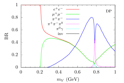
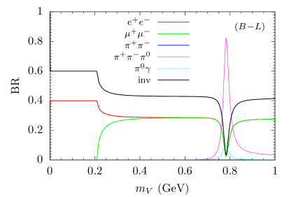
Figure 1: Decay ranching ratios (BR) as a function of the vector mass $m_{V}$ for a sub-GeV dark photon (left), or $B\!-\!L$ (right) vector boson.

2.2 Electromagnetic Injection Spectra

The analysis above shows that the relevant decay channels of the dark vectors of interest are: $e^{+}e^{-}$, $\mu^{+}\mu^{-}$, $\pi^{+}\pi^{-}$, $\pi^{+}\pi^{-}\pi^{0}$, $\pi^{0}\gamma$, $\nu\bar{\nu}$. These decays will all ultimately produce a collection of photons, electrons, and neutrinos. The resulting energy spectra of photons and electrons from these decay modes, in the lab frame where the decaying vector boson is at rest, are needed for our study of cosmological constraints to follow. Together, the full spectra per decay are

$$\frac{dN_{a}}{dE}\ =\ \sum_{i}\text{BR}(V\to i)\,\frac{dN_{a}^{(i)}}{dE}\ ,~{}~{}~{}~{}~{}a=\gamma,\,e,\,\nu$$ (16)

where the sum runs over the decay modes $i=e^{+}e^{-},\,\mu^{+}\mu^{-},\;\ldots$, and $e$ refers to the sum of electrons and positrons. We compute the spectra for each of the exclusive decay modes here, concentrating on the electrons and photons produced at leading non-trivial order. Our analysis is similar to that of Ref. [103] with some differences and additions. See also Ref. [104] for an alternate approach based on HERWIG 7 [116].

$\mathbf{V\to e^{+}e^{-}}$

This channel was considered previously in Ref. [95]. The leading-order electron spectrum is trivial with two electrons, each with energy $E=m_{V}/2$,

$$\frac{dN_{e}}{dE}=2\;\delta(E-m_{V}/2)\ .$$ (17)

In addition to electrons, photons can be produced from final-state-radiation (FSR). Following Ref. [103], we use the spectrum per decay

$$\left.\frac{dN_{\gamma}}{dE}\right|_{FSR} = \left(\frac{2}{m_{V}}\right)\frac{\alpha}{\pi}\,\frac{1}{(1+2\mu_{f}^{2})\sqrt{1-4\mu_{f}^{2}}}\;\frac{1}{x}\;\Bigg{(}$$

$${}\hskip 14.22636pt\left[1+(1-x)^{2}-4\mu_{f}^{2}(x+2\mu_{f}^{2})\right]\ln\!\left(\frac{1+\mathcal{W}_{f}}{1-\mathcal{W}_{f}}\right)$$

$${}\hskip 65.44142pt-\left[1+(1-x)^{2}-4\mu_{f}^{2}(1-x)\right]\,\mathcal{W}_{f}\Bigg{)}\ ,$$

with $x=E_{\gamma}/(m_{V}/2)$, $\mu_{f}=m_{f}/m_{V}$, and $\mathcal{W}_{f}=\sqrt{1-4\mu_{f}^{2}/(1-x)}$. As shown in Ref. [95], these FSR photons can have an important effect on BBN for sub-GeV injection.

$\mathbf{V\to\mu^{+}\mu^{-}}$

At leading order, this channel ultimately produces two electrons and four neutrinos. Beyond leading order, photons can be created through FSR and radiative muon decays.

To obtain the leading-order energy spectrum of electrons in the vector boson lab frame, we focus on the dominant $\mu^{-}\to e^{-}\bar{\nu}_{e}\nu_{\mu}$ decay channel. In the muon rest frame, for muon polarization $P\in[-1,1]$, the electron energy spectrum is the well-known Michel form [117, 118]:

$$\left.\frac{dN_{e}}{dE^{\prime}}\right|_{\mu}=\frac{2}{m_{\mu}}\,2{y^{\prime}}^{2}\left[(3-2y^{\prime})+P(1-2y^{\prime})\,\cos\vartheta\right]\,\Theta(1-y^{\prime})\ ,$$ (19)

where $y^{\prime}=2E^{\prime}/m_{\mu}$ and $\vartheta$ is the angle between the electron direction and the polarization axis in this frame. For anti-muon decays, the same spectrum applies but with the sign of $P$ reversed. However, for $V\to\mu^{+}\mu^{-}$ the net effect of muon polarization cancels and this term can be neglected. To get the lab frame spectrum we must boost the muon rest frame with Lorentz factor $\gamma=m_{V}/2m_{\mu}=1/\sqrt{1-\beta^{2}}$. Choosing the $z$ axis to lie along the muon boost direction and assuming the electron is emitted at polar angle $\theta^{\prime}$ from this axis in the muon rest frame, the electron energy and momenta in the lab frame are

$$E=\gamma(E^{\prime}+\beta\,p^{\prime}\cos\theta^{\prime})\ ,~{}~{}~{}p_{z}=\gamma(p^{\prime}\cos\theta^{\prime}+\beta E^{\prime})\ ,~{}~{}~{}p_{x}=p^{\prime}_{x}\ ,~{}~{}~{}p_{y}=p^{\prime}_{y}\ .$$ (20)

Changing variables from $(E^{\prime},\Omega^{\prime})$ to $(E,\Omega^{\prime})$ for solid angle $\Omega^{\prime}$ in the muon frame, we obtain the full lab frame distribution

$$\frac{dN_{e}}{dE}=\frac{2}{4\pi}\int\!d\Omega^{\prime}\;\frac{1}{\gamma(1+\beta\cos\theta^{\prime}\,E^{\prime}/p^{\prime})}\>\left.\frac{dN_{e}}{dE^{\prime}}\right|_{\mu}\ ,$$ (21)

where $E^{\prime}=E^{\prime}(E,\Omega)$, the first term in the integrand is the relevant Jacobian factor, the factor of $1/4\pi$ normalizes the solid angle integral, and the factor of two counts the identical contributions from the $\mu^{-}$ and $\mu^{+}$ branches.

The photon spectrum from muon decays is computed following Refs. [103, 119] as a sum of FSR and radiative contributions,

$$\frac{dN_{\gamma}}{dE}=\left.\frac{dN_{\gamma}}{dE}\right|_{\text{FSR}}+\left.\frac{dN_{\gamma}}{dE}\right|_{\text{rad}}\ .$$ (22)

This approach neglects interference between the two channels, but this effect is expected to be very small due to the narrow width of the muon. We use the expression of Eq. (2.2) with $m_{f}=m_{\mu}$ for the FSR part. The radiative spectrum is the sum of contributions from the $\mu^{+}$ and $\mu^{-}$ decays. In the muon rest frame, both are equal to [103, 119, 120]

$$\left.\frac{dN_{\gamma}}{dE^{\prime}}\right|_{\mu,\,rad} = \left(\frac{2}{m_{\mu}}\right)\frac{\alpha}{36\pi}\left(\frac{1-x}{x}\right)\Theta(1-x-r)$$

$${}\times\Bigg{(}12\big{[}3-2x(1-x)^{2}\big{]}\ln\!\left(\frac{1-x}{r}\right)+x(1-x)(46-55x)-102\Bigg{)}\ ,$$

where $x=2E^{\prime}/m_{\mu}$ and $r=(m_{e}/m_{\mu})^{2}$. The radiative photon spectrum in the lab frame is then obtained by boosting as in Eq. (21).

$\mathbf{V\to\pi^{+}\pi^{-}}$

Vector decays in this channel produce electrons primarily through the chain $\pi^{-}\to\bar{\nu}_{\mu}\mu^{-}$ with $\mu^{-}\to\nu_{\mu}\bar{\nu}_{e}e^{-}$ (and its conjugate). We focus on this chain exclusively since the inclusive branching $\text{BR}(\pi^{+}\to e^{+}{\nu}_{e})\simeq 1.2344\times 10^{-4}$ [121] is small enough to be numerically insignificant in our analysis. Photons are also produced through FSR and intermediate radiative decays.

To obtain the leading-order electron spectrum, we focus on the $\pi^{-}$ branch with $\pi^{-}\to\bar{\nu}_{\mu}\mu^{-}$ since an identical contribution arises for the $\pi^{+}$ branch. In the $\pi^{-}$ rest frame, the $\mu^{-}$ is produced with Lorentz factor

$$\gamma^{\prime}=\left(\frac{m_{\pi}}{2m_{\mu}}\right)\left(1+\frac{m_{\mu}^{2}}{m_{\pi}^{2}}\right)\ .$$ (24)

Aligning the $z$-axis with the direction of the outgoing muon, the muon obtains polarization $P=+1$. Defining $E^{\prime\prime}$ as the electron energy in the muon rest frame and $\theta^{\prime\prime}$ as the electron direction relative to the $z$-axis, the energy spectrum in this frame is given by Eq. (19) (with $E^{\prime}\to E^{\prime\prime}$ and $\theta^{\prime}\to\theta^{\prime\prime}$). The electron energy $E^{\prime}$ spectrum in the pion rest frame then follows from the boosting method described above with

$$E^{\prime}=\gamma^{\prime}(E^{\prime\prime}+\beta^{\prime}p^{\prime\prime}\cos\theta^{\prime\prime})\ ,~{}~{}~{}p_{z}^{\prime}=\gamma^{\prime}(p^{\prime\prime}\cos\theta^{\prime\prime}+\beta^{\prime}E^{\prime\prime})\ ,~{}~{}~{}p_{x}^{\prime}=p^{\prime\prime}_{x}\ ,~{}~{}~{}p_{y}^{\prime}=p^{\prime\prime}_{y}\ .$$ (25)

One more boost in an arbitrary pion direction $\hat{n}=(\sin\alpha\,\cos\phi,\sin\alpha\sin\phi,\cos\alpha)$ with Lorentz factor $\gamma=m_{V}/2m_{\pi}=1/\sqrt{1-\beta^{2}}$ is needed to transform to the lab frame where the vector is at rest. The electron energy in this frame is

$$E=\gamma\,E^{\prime}\left[1+\beta(\sin\alpha\cos\phi\sin\theta^{\prime}+\cos\alpha\,\cos\theta^{\prime})\right]\ ,$$ (26)

with

$$\cos\theta^{\prime}=\frac{\cos\theta^{\prime\prime}+\beta}{1+\beta\cos\theta^{\prime\prime}}\ .$$ (27)

The lab frame electron energy distribution is then obtained by a simple change of variables using uniform distributions for $\cos\theta^{\prime\prime}\in[-1,1]$, $\cos\alpha\in[-1,1]$, $\phi\in[0,2\pi]$, and $E^{\prime\prime}$ given by the Michel spectrum of Eq. (19). Note that for the positron spectrum from antimuon decays, the positron polarization is $P=-1$ while the sign of the $P$ term in the Michel spectrum is reversed leading to the same distribution in $E^{\prime\prime}$ and $\cos\theta^{\prime\prime}$.

The photon spectrum from this vector decay channel is obtained from a combination of FSR and internal radiative decays as in Eq. (22). For the FSR part, from the $V\to\pi^{+}\pi^{-}$ step, we use the result of Ref. [103],

$$\left.\frac{dN}{dE_{\gamma}}\right|_{\text{FSR}} = \left(\frac{2}{m_{V}}\right)\!\frac{2\alpha}{\pi}\,\frac{1}{(1-4\mu_{\pi}^{2})^{3/2}}\;\frac{1}{x}\;\Bigg{(}$$

$${}\hskip 14.22636pt(1-4\mu_{\pi}^{2})(1-x-2\mu_{\pi}^{2})\ln\!\left(\frac{1+{\cal W}_{\pi}}{1-{\cal W}_{\pi}}\right)$$

$${}\hskip 65.44142pt-[1-x-x^{2}-4\mu_{\pi}^{2}(1-x)]{\cal W}_{\pi}\Bigg{)}\ ,$$

where $x=E_{\gamma}/(m_{V}/2)$, $\mu_{\pi}=m_{\pi}/m_{V}$, and $\mathcal{W}_{\pi}=\sqrt{1-4\mu_{\pi}^{2}/(1/x)}$. The radiative contributions come from the $\pi^{-}\to\mu^{-}\bar{\nu}_{\mu}$ and $\mu^{-}\to e^{-}\bar{\nu}_{e}\nu_{\mu}$ steps of the decay chain. These were studied along with the radiative contribution from $\pi^{-}\to e^{-}\bar{\nu}_{e}$ in Ref. [103] where it was found that the total contribution is nearly completely dominated by the muon decay step. The contribution to the photon spectrum then follows by applying the boosting procedure described above to the photon spectrum of Eq. (2.2).

$\mathbf{V\to\pi^{0}\gamma}$

This channel produces a pair of boosted photons from the $\pi^{0}$ decay as well as a monochromatic photon directly. The $\pi^{0}$ and monochromatic photon energies in the lab frame are

$$E_{0}\ =\ \frac{m_{V}}{2}\left(1+\frac{m_{\pi^{0}}^{2}}{m_{V}^{2}}\right)\ ,~{}~{}~{}~{}~{}E_{\gamma}\ =\ \frac{m_{V}}{2}\left(1-\frac{m_{\pi^{0}}^{2}}{m_{V}^{2}}\right)\ .$$ (29)

For the photons from the $\pi^{0}$ decay, we have $E^{\prime}=m_{\pi^{0}}/2$ in the $\pi^{0}$ rest frame and a Lorentz factor $\gamma=E_{0}/{m_{\pi^{0}}}=1/\sqrt{1-\beta^{2}}$. Summing these contributions and applying our previous results, the full photon spectrum is therefore

$$\frac{dN_{\gamma}}{dE}\ =\ \delta(E-E_{\gamma})+\frac{2}{\beta\gamma\,m_{\pi^{0}}}\,B(E_{0})\ ,$$ (30)

where

$$B(E_{0}) = \Theta(E-(1-\beta)E_{0}/2)\;\Theta((1+\beta)E_{0}/2-E)$$ (34)

$$= \left\{\begin{array}[]{ccl}1&;&E~{}\in~{}[(1-\beta),\,(1+\beta)]\times(E_{0}/2)\\ 0&;&\text{otherwise}\end{array}\right.$$

$\mathbf{V\to\pi^{0}\pi^{+}\pi^{-}}$

For this channel we concentrate exclusively on the direct photons and electrons that arise from the dominant $\pi^{0}\to\gamma\gamma$ and $\pi^{-}\to\mu^{-}\bar{\nu}_{\mu}$, $\mu^{-}\to e^{-}\bar{\nu}_{e}\nu_{\mu}$ decay chains. The charged and neutral pions are created with a distribution of energies of

$$p_{3\pi}(E_{+},E_{-})\ =\ \frac{1}{\Gamma_{3\pi}}\,\frac{d^{2}\Gamma_{3\pi}}{dE_{+}dE_{-}}\ ,$$ (35)

with $E_{0}=m_{V}-E_{+}-E_{-}$, $\Gamma_{3\pi}$ given by Eq. (12), and $d^{2}\Gamma_{3\pi}/dE_{+}dE_{-}$ given by the same expression but with the function $\mathcal{I}(m_{V}^{2})$ replaced by the integrand of Eq. (2.1). The photon distribution is thus just the photon spectrum from a boosted $\pi^{0}$ decay found above weighted by the distribution of $\pi^{0}$ energies,

$$\frac{dN_{\gamma}}{dE}\ =\ \int\!dE_{+}\int\!dE_{-}\;p_{3\pi}(E_{+},E_{-})\,\frac{2}{\beta\gamma\,m_{\pi^{0}}}\,B(E_{0})\ ,$$ (36)

with $\gamma=1/\sqrt{1-\beta^{2}}=E_{0}/m_{\pi^{0}}$ and $B(E_{0})$ from Eq. (LABEL:eq:bfunc). Similarly, the electron (plus positron) spectrum is calculated using the boosted electron spectrum found previously for charged pion decay weighted by the joint distribution of $E_{+}$ and $E_{-}$ energies.

3 BBN Bounds on Sub-GeV Energy Injection

Energy injected into the cosmological plasma can disrupt the predictions of standard BBN by altering the ratio of neutrons to protons or by destroying/creating light elements after they are formed. In this section we study the photodissociation of light elements from electromagnetic energy injected by decays of long-lived sub-GeV dark vectors in the early universe. This is expected to be the most important effect of dark vector decays on BBN for decay lifetimes $\tau_{V}>10^{4}\,\text{s}$ and masses greater than a few MeV. We apply our results to constrain the pre-decay abundances of such vectors.

3.1 Methods for Calculating the Impact on BBN

Decays of sub-GeV dark vectors produce photons, electrons, and neutrinos, both directly and through intermediate muons and pions. To compute photodissociation effects from these decays, we make use of the branching fractions and the photon and electron energy spectra computed in the previous section. Note that for the cosmological times at which photodissociation is effective, $t\gtrsim 10^{4}\,\text{s}$, the muons and pions injected by sub-GeV vectors decay before they are slowed significantly by interactions with the cosmological background [44, 122].

Electrons and photons injected into the dense cosmological plasma generally interact with the plasma before reacting with light nuclei. The scattering of hard primaries off the background plasma creates an electromagnetic (EM) cascade that remains strongly suppressed until well after the main element creation stage of BBN has completed. Since the formation of the EM cascade is fast relative to the rate of scattering with nuclei, the resulting photon cascade spectrum can be treated as the source for subsequent photodissociation reactions on nuclei.

To compute the electromagnetic cascade spectra of photons and electrons (with positrons counted as electrons here), we follow the methods of Ref. [95] based on the earlier works of Refs. [98, 99]. Defining the differential number density per unit energy of photons or electrons in the cascade by

$$\mathcal{N}_{a}\ =\ \frac{dn_{a}}{dE}\ ,~{}~{}~{}~{}~{}a=\gamma,\,e$$ (37)

the cascade spectra evolve according to

$$\frac{d\mathcal{N}_{a}}{dt}(E)=-\Gamma_{a}(E)\mathcal{N}_{a}(E)+\mathcal{S}_{a}(E)\ ,$$ (38)

where $\Gamma_{a}$ is the net damping rate for species $a$ and energy $E$ and $\mathcal{S}_{a}(E)$ is the injection rate from all sources at this energy. The relevant damping and transfer reactions are generally fast relative to the Hubble rate and the effective photodissociation rates with light nuclei, and therefore the quasistatic limit of $d\mathcal{N}_{a}/dt\to 0$ is a good approximation [42]. This gives

$$\mathcal{N}_{a}(E)=\frac{\mathcal{S}_{a}(E)}{\Gamma_{a}(E)}\ ,$$ (39)

with both terms varying adiabatically as functions of time (or temperature).

The damping rate $\Gamma_{a}$ in Eq. (38) describes any reaction that transfers energy from species $a$ at energy $E$ to lower energies. The source terms in the electromagnetic cascade receive contributions from direct injection as well as from transfer reactions moving energy from higher up in the cascade down to energy $E$. Together, these take the explicit forms

$$\mathcal{S}_{a}(E)=R\,\frac{dN_{a}}{dE}+\sum_{b}\int_{E}^{E_{X}}\!dE^{\prime}\;K_{ab}(E,E^{\prime})\,\mathcal{N}_{b}(E^{\prime})\ ,$$ (40)

where $R$ is the injection rate, $dN_{a}/dE$ is the primary energy spectrum per injection, $E_{X}$ is the maximum energy in the cascade, and $K_{ab}(E,E^{\prime})$ is transfer kernel describing reactions $b(E^{\prime})+X_{BG}\to a(E)+X^{\prime}_{BG}$ within the cascade. In the case of energy injection from the decays of species $V$, $E_{X}\leq m_{V}/2$ and the injection rate is

$$R=\frac{n_{V}^{0}}{\tau_{V}}\,e^{-t/\tau_{V}}\ ,$$ (41)

where $\tau_{V}$ is the decay lifetime and $n_{V}^{0}$ is the number density the species would have in the in the absence of decays.

Multiple reactions contribute to the damping and source terms in the cascade. For photons, the dominant contribution to damping at higher energies $E\geq E_{c}\equiv m_{e}^{2}/22T$ is the photon-photon pair production (4P) reaction, $\gamma+\gamma_{BG}\to e^{+}+e^{-}$ [99]. In the case of electrons, at the relevant energies damping is dominated by inverse Compton (IC) scattering $e^{\mp}+\gamma_{BG}\to e^{\mp}+\gamma$ [123]. Together, these processes strongly suppress the electromagnetic cascade below nuclear dissociation thresholds until after the period of element formation, with $E_{c}>2\,\,{\rm MeV}$ only for $T\lesssim 6\,\,\mathrm{keV}$ ($t\gtrsim 7600\,\text{s}$). As a result, BBN bounds on electromagnetic injection from decay fall off very quickly for lifetimes $\tau_{V}\lesssim 10^{4}\,\mathrm{s}$.

For very high-energy initial injection, with $E_{X}T\gg m_{e}^{2}$, the photon cascade spectrum resulting from the 4P, IC, and other reactions is found to have a universal form. Specifically, the universal photon spectrum depends only on the total amount of electromagnetic energy injected into the cosmological plasma, and not on the detailed injection spectra or whether it came in the form or photons or electrons [98, 99]. However, recent studies of electromagnetic injection at lower energies have found significant deviations from universality [95, 100, 101, 102]. These deviations typically occur when the primary injection energy falls below the 4P cutoff $E_{c}$ or nuclear dissociation thresholds. For the sub-GeV dark vectors of interest in this work, we find that this takes place throughout a very significant portion of the relevant parameter space. More details on deviations from universality and when it occurs are collected in Ref. [95] and Appendix A.

With the photon cascade spectrum in hand, the effect of photodissociation on the light element abundances can be described by Boltzmann equations of the form

$$\frac{dY_{A}}{dt}=\sum_{i}Y_{i}\int_{0}^{\infty}\!dE_{\gamma}\,\mathcal{N}_{\gamma}(E_{\gamma})\,\sigma_{\gamma+i\to A}(E_{\gamma})-Y_{A}\sum_{f}\int_{0}^{\infty}\!\;dE_{\gamma}\,\mathcal{N}_{\gamma}(E_{\gamma})\,\sigma_{\gamma+A\to f}(E_{\gamma})\ ,$$ (42)

where $\mathcal{N}_{\gamma}(E_{\gamma})$ are the photon cascade spectra, $A$ and the sums run over the relevant isotopes, and $Y_{A}$ are isotope number densities normalized to the entropy density,

$$Y_{A}=\frac{n_{A}}{s}\ .$$ (43)

Reactions initiated by electrons are not included because their cascade spectrum is always strongly suppressed by IC scattering.

The nuclear species included in our analysis are hydrogen (H), deuterium ($\mathrm{D}={}^{2}\mathrm{H}$), tritium ($\mathrm{T}={}^{3}\mathrm{H}$), helium-3 (${}^{3}\mathrm{He}$), and helium ($\mathrm{He}={}^{4}\mathrm{He}$). Heavier species such as lithium have much smaller primordial abundances and their inclusion would not alter our results for the light elements we consider. For the nuclear cross sections in Eq. (42), we use the simple parametrizations collected in Ref. [42]. These cross sections all have the same general shape with a sharp rise at threshold up to a peak followed by a smooth fall off. The two most important thresholds for our study are $E_{th}\simeq 2.22\,\,{\rm MeV}$ for deuterium photodissociation and $E_{th}\simeq 19.81\,\,{\rm MeV}$ for helium, with the other relevant reaction thresholds typically in the range of $E_{th}\sim 2.5-8.5\,\,{\rm MeV}$.

To solve the coupled evolution equations of Eq. (42), we convert time to redshift and use initial primordial abundances expected from standard BBN predicted by PArthENoPE [124, 125]:

$$Y_{p}=0.247\ ,~{}~{}~{}~{}~{}\frac{n_{\mathrm{D}}}{n_{\mathrm{H}}}=2.45\times 10^{-5}\ ,~{}~{}~{}~{}~{}\frac{n_{{}^{3}\mathrm{He}}}{n_{\mathrm{H}}}=0.998\times 10^{-5}\ .$$ (44)

We then compare the resulting light element abundances to the following observed values, quoted with effective $1\sigma$ uncertainties (with theoretical and experimental uncertainties combined in quadrature):

$$Y_{p} = 0.245\pm 0.004\hskip 63.16515pt(\text{Ref.~{}\cite[cite]{[\@@bibref{}{Aver:2015iza}{}{}]}})$$ (45)

$$\frac{n_{\mathrm{D}}}{n_{\mathrm{H}}} = (2.53\pm 0.05)\times 10^{-5}\hskip 28.45274pt(\text{Ref.~{}\cite[cite]{[\@@bibref{}{Cooke:2017cwo}{}{}]}})$$ (46)

$$\frac{n_{{}^{3}\mathrm{He}}}{n_{\mathrm{H}}} = (1.0\pm 0.5)\times 10^{-5}\hskip 39.83368pt(\text{Ref.~{}\cite[cite]{[\@@bibref{}{Geiss:2003ab}{}{}]}})\ .$$ (47)

The helium mass fraction $Y_{p}$ we use is consistent with Ref. [129] and earlier determinations but significantly lower than the result of Ref. [130]. The uncertainty on the ratio $n_{\mathrm{D}}/{n_{\mathrm{H}}}$ is dominated by a theory uncertainty on the rate of photon capture on deuterium from Ref. [131]. For $n_{{}^{3}\mathrm{He}}/n_{\mathrm{H}}$, we use the determination of $(n_{\mathrm{D}}+n_{{}^{3}\mathrm{He}})/n_{\mathrm{H}}$ of Ref. [128] along with the value of $n_{\mathrm{D}}/{n_{\mathrm{H}}}$ from Ref. [127]. The uncertainties quoted here are generous, and in the analysis below we implement exclusions at the 2$\sigma$ level.

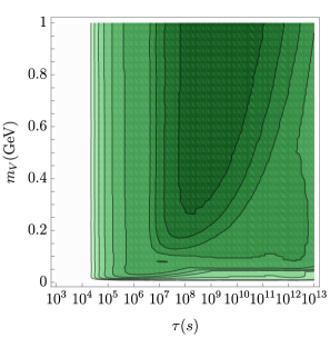
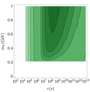
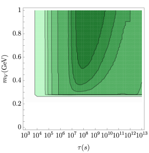
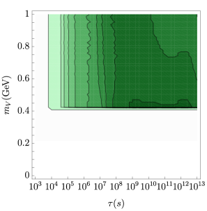
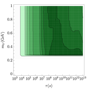
Figure 2: BBN upper limits from electromagnetic effects on the mass times yield $\log_{10}(m_{V}Y_{V}/\,{\rm GeV})$ of a sub-GeV decaying particle $V$ in the lifetime-mass plane for the exclusive decays $V\to e^{+}e^{-}$ (upper left), $V\to\mu^{+}\mu^{-}$ (upper right), $V\to\pi^{+}\pi^{-}$ (lower left), $V\to\pi^{+}\pi^{-}\pi^{0}$ (lower middle), and $V\to\pi^{0}\gamma$ (lower right).

To illustrate our approach, we show in Fig. 2 the photodissociation bounds from BBN on the pre-decay yield $Y_{V}=n_{V}/s$ for a decaying species $V$ with mass $m_{V}$ and lifetime $\tau_{V}$ assuming that all decays occur exclusively via one of the channels $V\to e^{+}e^{-}$, $\mu^{+}\mu^{-}$, $\pi^{+}\pi^{-}$, $\pi^{0}\pi^{+}\pi^{-}$, $\pi^{0}\gamma$. Decays to $e^{+}e^{-}$ produce the strongest effect throughout most of the lifetime–mass plane shown. Relative to the $\mu^{+}\mu^{-}$ and $\pi^{+}\pi^{-}$ channels, electron decays produce more energetic electrons and a greater electromagnetic injection fraction. At lower masses and larger lifetimes, in the lower right region of the plots, the injected electrons scatter off background photons in the Thomson regime where the upscattered photons receive energies well below nuclear photodissociation thresholds. The dominant sources of photons contributing to photodissociation are then FSR and radiative decays, and these also tend to be greater for $e^{+}e^{-}$ than $\mu^{+}\mu^{-}$ or $\pi^{+}\pi^{-}$ channels. This obstacle does not affect the $\pi^{0}\pi^{+}\pi^{-}$ and $\pi^{0}\gamma$ channels which produce photons at the leading order and thus stronger BBN limits in the lower right region of the plots. Note that even after rescaling by the total electromagnetic fractions produced by these various modes, the resulting BBN limits are significantly different, reflecting the breaking of universality of the cascade photon spectrum, as discussed in more detail in Appendix A.

3.2 BBN Bounds on Dark Vectors

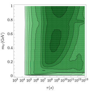
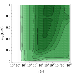
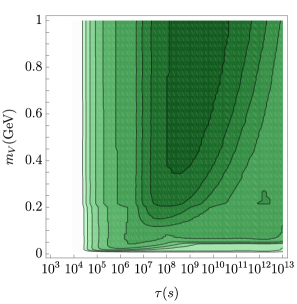
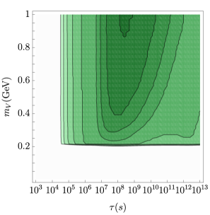
Figure 3: BBN upper limits from electromagnetic effects on the mass times yield $\log_{10}(m_{V}Y_{V}/\,{\rm GeV})$ of sub-GeV dark vectors in the lifetime-mass plane for the dark vector species DP (upper left), $B\!-\!L$ (upper middle), $L_{e}\!-\!L_{\mu}$ (lower left), $L_{e}\!-\!L_{\tau}$ (lower middle), and $L_{\mu}\!-\!L_{\tau}$ (lower right).

Using the dark vector decay fractions and the BBN methods described above, we can now derive BBN limits due to photodissociation on the pre-decay yield $Y_{V}=n_{V}/s$ of a dark vector with mass $m_{V}$ and lifetime $\tau_{V}$. Our results are shown in Fig. 3 for the dark vector species DP (upper left), $B\!-\!L$ (upper middle), $L_{e}\!-\!L_{\mu}$ (lower left), $L_{e}\!-\!L_{\tau}$ (lower middle), and $L_{\mu}\!-\!L_{\tau}$ (lower right). The shapes of these exclusions can be understood by comparing the branching fractions shown in Fig. 1 and the bounds on the contributing decay modes in Fig. 2. For the dark photon (DP) and $B\!-\!L$ vectors, the bounds get weaker due to hadronic contributions near the $\rho$ and $\omega$ resonances. This effect is greater for the DP due to its strong mixing with the wide $\rho$ resonance relative to the $B\!-\!L$ that approximately only mixes with the narrow $\omega$. With the exception of the DP, an increase in the bound is seen near the muon threshold at $m_{V}=2m_{\mu}$ due to the larger visible mode decay branching fractions when the muon channel turns on and a smaller fraction of the decays go to neutrinos. For the $L_{\mu}\!-\!L_{\tau}$ vector, the bounds below the muon threshold fall beneath the range covered by the figure since the decay products in this region are nearly completely dominated by neutrinos.

In addition to photodissociation, dark vector decays can also modify the outcome of standand BBN by altering the ratio of neutrons to protons and through the hadrodissociation of light elements. While these effects can be significant and further constrain the properties of dark vectors, we argue that they are also largely orthogonal to the bounds from photodissociation derived above. Lighter dark vectors with $m_{V}\lesssim 20\,\,{\rm MeV}$ can alter the effective number of light degrees of freedom during and after neutron-proton freeze-out through their direct influence [29], from their decays following neutrino decoupling [29, 132], or by equilibrating light right-handed neutrinos (which we assume to not be present) [90, 133]. The couplings required for these effects to be significant correspond to dark vector lifetimes below $\tau_{V}\lesssim 10^{4}\,\text{s}$, or large initial densities $m_{V}Y_{V}\gg 10^{-9}$, and thus these considerations apply to earlier decays or produce weaker constraints than photodissociation. Heavier dark vectors that decay to pions can alter the neutron to proton ratio through reactions such as $p+\pi^{-}\to n+\pi^{0}$ or destroy light elements through hadrodissociation. The analyses of Refs. [86, 87, 122] find that these effects are strongest for lifetimes $\tau_{V}\sim 10^{3}\,\mathrm{s}$ and $m_{V}Y_{V}\gtrsim 10^{-11}\,\,{\rm GeV}$. Comparing to our results for photodissociation, these two sets of bounds largely apply independently of one another, with only a very small region of possible interference near $\tau_{V}\sim 10^{4}\,\text{s}$. Taken together, these considerations justify our earlier treatment of photodissociation bounds from BBN in isolation.

4 CMB Bounds on Sub-GeV Energy Injection

Energy injection in the early universe can also modify the power and freqency spectra of the CMB. In this section we describe the methods that we use to compute these effects and show the constraints they imply for dark vector decays.

4.1 Methods for the CMB Power Spectrum

Energy injected during and after recombination can ionize newly-formed atoms and broaden the surface of last scattering. These effects can modify the power spectra of CMB fluctuations relative to the standard recombination history [56]. Precision measurements of the CMB power spectra can therefore be used to constrain new sources of energy injection in this period [57, 58].

The total rate of energy injection per unit volume from a decaying species of mass $m_{V}$ is simply $m_{V}R$, where $R$ is the decay rate per unit volume given in Eq. (41). For decays near or after recombination, there may be a delay between the initial decay and when the resulting energy is deposited within the cosmological medium [59]. We treat this as in Refs. [134, 135] and write the total energy deposition rate per unit volume as

$$\left(\frac{d\rho}{dt}\right)_{\!\!dep}=f(z)\,\frac{m_{V}n_{V}^{0}}{\tau_{V}}\ ,$$ (48)

where $n_{V}^{0}$ is the number density in the absence of decays and

$$f(z)=\frac{H(z)\sum_{a}\int_{\ln(1+z)}^{\infty}\!\frac{d\ln(1+z^{\prime})}{H(z^{\prime})}\int\!dE\;T^{(a)}(z^{\prime},z,E)\,E\,\frac{dN_{a}}{dE}\,e^{-t(z^{\prime})/\tau_{V}}}{\sum_{b}\int\!dE\;E\,\frac{dN_{b}}{dE}}\ .$$ (49)

Here, $dN_{a}/dE$ are the energy spectra per decay, with the sum in the numerator running over $a=e,\gamma$ and the sum in the denominator over $b=e,\gamma,\nu$. The $T^{(a)}(z^{\prime},z,E)$ are transfer functions that describe the fraction of energy deposited at $z$ for injection at energy $E$ and redshift $z^{\prime}\leq z$. Note that the exponential depletion due to decays has been incorporated into the deposition function $f(z)$ as in Ref. [135].

In addition to the total efficiency of energy deposition described by $f(z)$, similar functions $f_{i}(z)$ and corresponding transfer functions $T_{i}^{{(a)}}$ can be defined for energy deposition into specific channels such as hydrogen ionization, helium ionization, heating of the cosmological medium, and photons with energies below $10.2\,\text{eV}$ that free-stream [136]. Arrays of these transfer functions are collected in Ref. [137] and we apply them to our analysis. The effect of energy injection on the CMB power spectra is almost entirely due to the ionization of hydrogen, with much smaller contributions from helium ionization and Lyman-$\alpha$ photons [138]. As in Ref. [136], we define an ionization fraction $\chi_{ion}$ by

$$\chi_{ion}(z)=f_{ion}(z)/f(z)\ ,$$ (50)

where $f_{ion}$ is the total efficiency of depositing energy into the ionization of hydrogen and helium.

A powerful method to connect the energy deposition function $f(z)$ to bounds from CMB measurements was derived in Ref. [139] based on a principal component method. In this approach, orthogonal eigenfunctions with respect to the space of energy deposition histories are obtained from data (or data projections) that characterize the impact of energy injection on the CMB power spectra, with a marginalization over $\Lambda\text{CDM}$ parameters included. The significance of the energy injection is then given by the orthogonal sum over the expansion coefficients of $f(z)$ with respect to the eigenfunction basis weighted by their corresponding eigenvalues. Ordering the eigenfunctions by the sizes of their eigenvalues, only a small set of these principal components need to be included to get an excellent approximation of the full result [139] (which requires a intensive computation with tools such as CLASS [140] and CosmoMC [141] for each model of interest).

To estimate the CMB bounds from Planck [4] on dark vector decays, we make use of principal component functions and eigenvectors over the space of energy deposition histories described in Refs. [134, 139, 142] and collected in Ref. [137]. These were computed in Ref. [139] using the ionization fraction $\chi_{base}(z)$ formulated in Refs. [56, 143]. This was subsequently improved in Ref. [136] to account for losses to photons with energies below $10.2\,\text{eV}$ that do not contribute to ionization. To implement this improvement, we follow the prescription of Refs. [144, 145, 146] by replacing $f(z)$ in the analysis with

$$\tilde{f}(z)\ =\ {\chi_{c}(z)}f(z)\Big{/}{\chi_{base}(z)}\ .$$ (51)

With this prescription, we estimate the bounds from Planck and make projections for a cosmic variance limited (CVL) experiment with multipoles up to $\ell=2500$ using the principal component functions of Ref. [137]. In the case of Planck, these functions were derived based on a projection of the experimental sensitivity rather than data [137, 139]. However, this projection turns out to be remarkably accurate at predicting the limits on $s$-wave dark matter annihilation derived from the Planck 2015 [147] and Planck 2018 [4] data sets. For decays, we also find that the projected limits for longer lifetimes $\tau_{V}\gg 10^{13}\,\text{s}$ agree well with the principal components derived for dark matter decay with respect to the space of energy injection spectra based on Planck 2015 data [146].

4.2 Methods for the CMB Frequency Spectrum

Late-time energy injection can also distort the CMB frequency spectrum [53, 54] from the nearly perfect blackbody that is observed [148]. For decays after the decoupling of double-Compton scattering at redshift $z_{th}\simeq 2.0\times 10^{6}$ but before the decoupling of Compton scattering at $z_{C}\simeq 5.2\times 10^{4}$, the decay products equilibrate kinetically but generate an effective photon chemical potential [53, 54]. Decays after Compton decoupling but before recombination at $z_{rec}\simeq 1090$ produce a distortion that can be described by the Compton $y$ parameter [53, 54]. The current limits on $\mu$ and $y$ from COBE/FIRAS are [148]

$$\mu<9\times 10^{-5},~{}~{}~{}~{}~{}|y|<1.5\times 10^{-5}\ ,$$ (52)

while the proposed PIXIE satellite is projected to have sensitivity to constrain [149]

$$\mu<1\times 10^{-8},~{}~{}~{}~{}~{}|y|<2\times 10^{-9}\ .$$ (53)

These limits can be used to constrain decays in the early universe.

An accurate expression for both types of distortions is [150, 151, 152, 153]

$$\frac{\mu}{1.401} \simeq \int\!dt\;\mathcal{J}_{\mu}\left(\frac{\Delta\dot{\rho}_{\gamma}}{\rho_{\gamma}}\right)$$ (54)

$$\frac{y}{1/4}~{} \simeq \int\!dt\;\mathcal{J}_{y}\left(\frac{\Delta\dot{\rho}_{\gamma}}{\rho_{\gamma}}\right)$$ (55)

where the $\mathcal{J}_{i}$ are window functions, $\rho_{\gamma}$ is the energy density of photons, and $\Delta\dot{\rho}_{\gamma}$ is the rate of electromagnetic energy injection per unit volume. For the window functions, we use “method C” of Ref. [153]:

$$\mathcal{J}_{\mu}(z) = e^{-(z/z_{th})^{5/2}}\,\left[1-\exp\left(-\Big{[}(1+z)/5.8\times 10^{4}\Big{]}^{1.88}\right)\right]$$ (56)

$$\mathcal{J}_{y}(z) = \left(1+\Big{[}({1+z})/{6\times 10^{4}}\Big{]}\right)^{-1}\Theta(z-z_{rec})\ .$$ (57)

The energy injection profile for a decaying dark vector is $\Delta\dot{\rho}_{\gamma}=f_{em}m_{V}R$, with $R$ given by Eq. (41), and $f_{em}$ the electromagnetic energy fraction of the decay. For sub-GeV dark vectors we approximate this fraction by

$$f_{em}\ \simeq\ \text{BR}(e^{+}e^{-})+\frac{1}{3}\,\text{BR}(\mu^{+}\mu^{-})+\frac{1}{4}\,\text{BR}(\pi^{+}\pi^{-})+\frac{1}{2}\,\text{BR}(\pi^{+}\pi^{-}\pi^{0})+\text{BR}(\pi^{0}\gamma)\ .$$ (58)

Note that in contrast to the BBN and CMB power spectrum bounds discussed above, this constraint on decaying particles is largely insentive to the energy spectrum of the decays.

4.3 CMB Bounds on Dark Vectors

In Fig. 4 we show the estimated bounds from deviations in the CMB power spectrum relative to Planck measurements on the pre-decay dark vector yield $Y_{V}=n_{V}/s$ as a function of decay lifetime $\tau_{V}$ and mass $m_{V}$ for the dark vector species DP (upper left), $B\!-\!L$ (upper middle), $L_{e}\!-\!L_{\mu}$ (lower left), $L_{e}\!-\!L_{\tau}$ (lower middle), and $L_{\mu}\!-\!L_{\tau}$ (lower right). We note that these bounds constrain values of $m_{V}Y_{V}$ that are orders of magnitude lower than from BBN. However, the CMB constraints fall off quickly for lifetimes below $\tau_{V}\lesssim 10^{13}\,\text{s}$ and BBN becomes more important. Let us also emphasize that the results shown for $\tau_{V}\lesssim 10^{13}\,\text{s}$ have a very significant theoretical uncertainty that we do not attempt to estimate (see also Refs. [135, 139, 146]). The shape of the CMB bounds mirrors those from BBN, with direct photon and electron injection having a greater impact than muons or charged pions, and thus the emergence of muon decays and hadronic resonances with increasing dark vector mass produce distinct features in the figures.

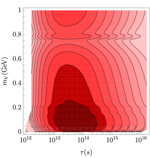
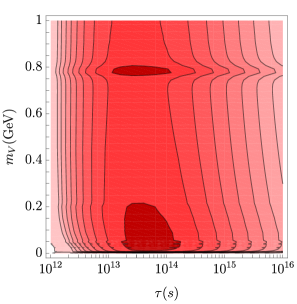
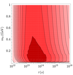
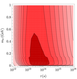
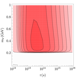
Figure 4: Estimated CMB upper bounds from Planck on the mass times yield $\log_{10}(m_{V}Y_{V}/\,{\rm GeV})$ of sub-GeV dark vectors in the lifetime-mass plane for the dark vector species DP (upper left), $B\!-\!L$ (upper middle), $L_{e}\!-\!L_{\mu}$ (lower left), $L_{e}\!-\!L_{\tau}$ (lower middle), and $L_{\mu}\!-\!L_{\tau}$ (lower right).

In the left panel of Fig. 5 we show the approximately mass-independent bounds on the combination $f_{em}m_{V}Y_{V}$ from $\mu$- and $y$-type distortions of the CMB frequency spectrum from COBE/FIRAS measurements as well as projected constraints from PIXIE. The $\mu$-type distortions are dominant prior to the freezeout of double-Compton scattering, and $y$-type distortions become more important after that. To convert the curves in the left panel into bounds on a specific dark vector theory, it is only a matter of determining $f_{em}$. In the right panel of Fig. 5 we plot $f_{em}$ as a function of mass $m_{V}\in[\,{\rm MeV},\,{\rm GeV}]$ for the five dark vector varieties discussed above. Relative to BBN electromagnetic effects, dark vector decays are constrained slightly more weakly by current data on the CMB frequency spectrum, but will become much more constraining with data from PIXIE. However, for $\tau_{V}\gtrsim 10^{13}\,\text{s}$, energy injection primarily alters the CMB power spectra rather than the frequency spectrum [58, 59], and the power spectra give the strongest limits.

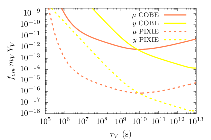
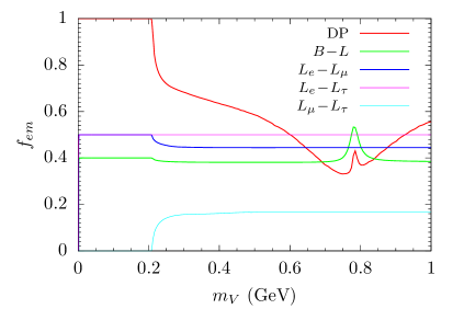
Figure 5: In the left panel we show current (projected) bounds from COBE/FIRAS (PIXIE) on the electromagnetic decay factor $f_{em}m_{V}Y_{V}$ from late-time vector decays as a function of the decay lifetime $\tau_{V}$. The right panel shows the electromagnetc decay fraction $f_{em}$ for the five dark vector theories studied in this work.

5 Cosmological Limits on Thermal Dark Vectors

Dark vector bosons can be created through a number of mechanisms in the early universe, including direct thermal production from SM collisions, decays or annihilations of other dark sector particles, or in reheating after inflation. In this section we investigate the thermal production of dark vectors since it provides the (nearly) lowest possible dark vector population and thus the most model-independent bounds on them.

5.1 Thermal Production by Freeze-In

A minimal population of dark vectors will be created by thermal $N\to 1$ freeze-in reactions of the form $(\text{SM})^{N}\to V$. This production is described by

$$s\frac{dY_{V}}{dt}=\mathcal{C}[f_{V}]\ ,$$ (59)

where $s$ is the entropy density, $f_{V}$ is the distribution function of the dark vector species, and $\mathcal{C}[f_{V}]$ is the standard collision term [1]. For underpopulated dark vectors with $f_{V}\ll f_{V}^{eq}$ and neglecting Bose enhancement and Pauli blocking factors, detailed balance implies

$$\mathcal{C}[f_{V}]~{}=~{}3\int\!\frac{d^{3}p_{V}}{(2\pi)^{3}}\left(\frac{m_{V}}{E_{V}}\right)f_{V}^{eq}(p_{V})\,\Gamma_{V}~{}=~{}\left<\frac{1}{\gamma}\right>n_{V}^{eq}\Gamma_{V}\ ,$$ (60)

where $\Gamma_{V}$ is the total decay width in the $V$ rest frame and the brackets refer to the thermal average of the inverse Lorentz factor.

The collision term for dark photon production was computed including thermal corrections and full Fermi-Dirac statistics in Ref. [86]. There it was found that full calculation via leptons (or perturbative quarks) is approximated very well by evaluating the collision term with a Maxwell-Boltzmann distribution and neglecting thermal corrections. Using a Maxwell-Boltzmann form for $f_{V}^{eq}$ in Eq. (60), the integral can be evaluated analytically with the result [154, 155]

$$\mathcal{C}[f_{V}]~{}=~{}\frac{3}{2\pi^{2}}\,\Gamma_{V}\,m_{V}^{2}\,T\,K_{1}(m_{V}/T)\ ,$$ (61)

where $K_{1}$ is the modified Bessel function of the first kind.

To evaluate the thermal yield with this collision term, we follow Ref. [86] and convert time to $x=m_{V}/T$ and divide the production into temperatures above and below the QCD phase transition, assumed to occur at $\Lambda_{\text{QCD}}\simeq 157\,\,{\rm MeV}$. The net yield is then

$$Y_{V}=(Y_{V})_{I}+(Y_{V})_{II}\ ,$$ (62)

with

$$\left(Y_{V}\right)_{I} = \frac{3}{2\pi^{2}}\,m_{V}^{3}\,\tilde{\Gamma}_{V}\,\int_{0}^{x_{\text{QCD}}}\!dx\;\frac{K_{1}(x)}{x^{2}\,s\,H}$$ (63)

$$\left(Y_{V}\right)_{II} = \frac{3}{2\pi^{2}}\,m_{V}^{3}\,{\Gamma}_{V}\,\int_{x_{\text{QCD}}}^{\infty}\!dx\;\frac{K_{1}(x)}{x^{2}\,s\,H}\ ,$$ (64)

where $x_{\text{QCD}}=m_{V}/\Lambda_{\text{QCD}}$ and $\tilde{\Gamma}_{V}$ is the vector decay width into perturbative quark (and lepton) final states. For this, we consider up quarks with $m_{u}=2.2\,\,{\rm MeV}$, down quarks with $m_{d}=4.7\,\,{\rm MeV}$, and strange quarks with $m_{s}=93\,\,{\rm MeV}$ [118]. With this approach, our results for the yield of the dark photon agree well with Ref. [86]. To the extent that the number of relativistic degrees of freedom is constant during production and is dominated by $T<\Lambda_{\text{QCD}}$, the final dark vector yield is approximately [86]

$$Y_{V}~{}\simeq~{}\frac{9}{4\pi}\,\frac{m_{V}^{3}\Gamma_{V}}{(sH)_{x=1}}\ .$$ (65)

We use the full result of Eqs. (62,63,64) in the analysis to follow.

5.2 Cosmological Bounds on Thermal Dark Vector Parameters

By combining the thermal production yields with the BBN and CMB constraints derived previously, we can put limits on dark vectors produced thermally in the early universe. To compare the limits on various dark vector theories on an equal footing and to connect with previous work, it is convenient to define an effective coupling $\epsilon_{eff}$ by

$$\epsilon_{eff}=\left\{\begin{array}[]{ccl}\epsilon&;&\text{dark photon}\\ &&\\ \sqrt{\alpha_{V}/\alpha}&;&\text{direct-coupling vectors}\end{array}\right.$$ (69)

where $\alpha^{-1}\simeq 137.036$ is the usual fine-structure constant.

In Fig. 6 we show the BBN, CMB-power, and CMB-frequency exclusions from electromagnetic energy injection in the $m_{V}$–$\epsilon_{eff}$ plane on thermally-produced dark vector species. The four panels correspond to the dark vector species dark photon (upper left), $B\!-\!L$ (upper right), $L_{e}\!-\!L_{\mu}$ (lower left), and $L_{e}\!-\!L_{\tau}$ (lower right), all with dominant decays to the SM. The green shaded regions show the BBN exclusions from photodissiciation, the shaded red region gives the bound from Planck deviations in the CMB power spectra, the dashed red contour indicates the potential future sensitivity from a cosmic variance limited experiment up to $\ell=2500$, the solid yellow region shows the exclusion from COBE/FIRAS from distortions in the CMB frequency spectrum, and the dashed yellow contour shows the projected reach of PIXIE for such distortions. No significant exclusion is found for the $L_{\mu}\!-\!L_{\tau}$ vector. Let us also emphasize that these exclusions are conservative in the sense that they only rely on the assumption of an early universe dominated by SM radiation at temperature $T\gtrsim m_{V}$. The exclusions would be even stronger if there were other production sources for the dark vector such as particle decay or annihilation [84, 85, 102].

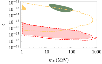
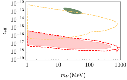
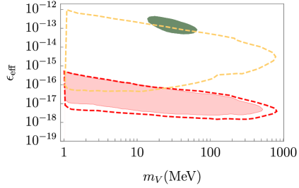
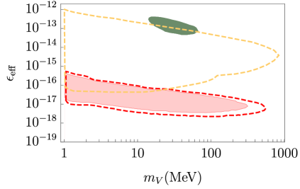
Figure 6: Cosmological limits on dark vectors from electromagnetic energy injection as a function of the dark vector mass $m_{V}$ and effective coupling $\epsilon_{eff}$ assuming a thermal freeze-in abundance. The dark vector varieties shown are a dark photon (upper left), $B\!-\!L$ (upper right), $L_{e}\!-\!L_{\mu}$ (lower left), and $L_{e}\!-\!L_{\tau}$ (lower right). The shaded green regions indicate the exclusions from BBN due to photodissociation, the shaded red regions show the exclusion from the CMB power spectrum measured by Planck, the dashed red contours indicate the projected limits for a cosmic variance limited experiment, the solid yellow region shows the exclusion from CMB frequency spectrum distortions in COBE/FIRAS, and the dashed yellow contours give the projected sensitivity to such distortions at PIXIE.

The cosmological limits we find for the dark photon are qualitatively similar to those derived in Refs. [86, 87]. Compared to these works, our analysis includes several updates that affect the detailed quantitative results for the dark photon and our study extends to other types of dark vectors. The most significant update is our treatment of electromagnetic energy injection and the resulting photon cascade spectrum relevant for BBN. In Ref. [86] the universal photon spectrum was used, while in Ref. [87] the modification of the photon spectrum from $e^{+}e^{-}$ injection due to the Thomson limit of inverse Compton scattering was included leading to much weaker exclusions from BBN photodissociation effects. Our result lies between these two exclusions – we confirm the suppression of the photon cascade spectrum from lower-energy $e^{+}e^{-}$ injection pointed out in Ref. [87] but we also find a significant (and sometimes dominant) additional contribution from final-state photon radiation in these decays that bring our result closer to Ref. [86]. In our treatment of deviations in the CMB power spectrum, we also use the updated treatment of the ionization fraction presented in Refs. [136, 138, 144, 146].

The parameter bounds presented in Fig. 6 are the strongest constraints on the species of (thermal) sub-GeV dark vectors studied here with $\epsilon\lesssim 10^{-12}$ and $m_{V}\lesssim\,{\rm GeV}$. For $\epsilon\sim 10^{-11}$ and $m_{V}\sim\,{\rm GeV}$, Refs. [86, 87] also found disjoint BBN exclusions on the dark photon from neutron-proton converstions induced by charged pion and kaon injection, while for $\epsilon\sim 10^{-13}$ and $m_{V}\gtrsim 2\,\,{\rm GeV}$ they obtained BBN bounds mainly from the direct injection of neutrons from vector decays. These BBN bounds from hadronic injection are expected to carry over similarly to the $B\!-\!L$ vector for masses above $m_{V}\gtrsim 1\,\,{\rm GeV}$. Dark vectors can also alter the effective number of relativistic neutrino species $N_{eff}$ by thermalizing light singlet neutrinos [90] or by injecting energy preferentially into either electromagnetic species or neutrinos after neutrino decoupling [21, 22, 23, 29, 132], with the corresponding bounds based on freeze-in production of a dark photon extending down to $\epsilon\lesssim 5\times 10^{-10}$ for $m_{V}\lesssim 8\,\,{\rm MeV}$. The emission of gamma-rays by the decays of dark vectors that would have been produced in supernova SN1987A [156, 157] was shown to rule out couplings down to $\epsilon_{eff}\sim 10^{-12}$ for masses between 1–100 MeV [157], independent of the cosmological production mechanism of the dark vector. Taken together, our cosmological exclusions of dark vectors (assuming freeze-in production) are disjoint from these others.

Beyond the limits shown above, we have also estimated the gamma-ray signals of dark vector decays with lifetimes longer than the age of the universe. Translating these signals to the equivalent from the decay of a long-lived particle making up all the DM, they correspond to effective DM lifetimes greater than $\tau_{eff}\gtrsim 10^{30}\,\text{s}$, well beyond the current limits of $\tau\gtrsim 10^{25}\,\text{s}$ for $\text{DM}\to e^{+}e^{-}$ in this mass region [158].

6 Conclusions

In this work we have investigated the cosmological bounds on a range of sub-GeV dark vectors based on the electromagnetic energy injected by their decays in the early universe. This injection can alter the SM+$\Lambda\text{CDM}$ predictions for the light element abundances from BBN and the power and frequency spectra of the CMB. Our work expands on previous studies of cosmological bounds on kinetically-mixed dark photons [86, 87], and extends them to four other dark vector species: $B\!-\!L$, $L_{e}\!-\!L_{\mu}$, $L_{e}\!-\!L_{\tau}$, and $L_{\mu}\!-\!L_{\tau}$.

The cosmological bounds we derive are based on electromagnetic energy injection. We take into account deviations from universality in electromagnetic effects on BBN from lower-energy injection by computing explicitly the development of the electromagnetic cascade photon spectrum. In doing so, we take into consideration the detailed photon and electron energy injection spectra including radiative effects such as FSR. For the specific case of a dark photon created through thermal freeze-in, the BBN bounds we find are slightly weaker than Ref. [86] and somewhat stronger than Ref. [87]. Our results for CMB exclusions on the dark photon appear to be in agreement with Refs. [86, 87], although we apply a more detailed energy injection spectrum and we update the effective ionization fraction following Ref. [144, 145, 146]. We also extend these methods to other dark vector species.

Relative to direct laboratory tests of dark vectors, the bounds we find from cosmology are able to constrain much smaller couplings to SM matter, with CMB bounds extending all the way to $\epsilon_{eff}\sim 10^{-18}$. For the dark photon, it is challenging to obtain kinetic mixings this small [159], but they can arise when there is an approximate charge conjugation ($C$) invariance within the dark sector [160] or collective symmetries [161]. For the other direct coupling vectors, the bounds on the gauge couplings we find from cosmology are strong enough to be potentially relevant for certain superstring swampland considerations, corresponding to the set of consistent low-energy effective theories that cannot be embedded into a consistent theory of quantum gravity [162, 163, 164]. In particular, $m_{V}\sim\,{\rm GeV}$ and $\epsilon_{eff}=\sqrt{\alpha_{V}/\alpha}\sim 10^{-18}$ approach the parameter range covered by the weak gravity conjecture proposed in Ref. [163].

Appendix A Appendix: Departures from EM Universality in BBN

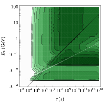
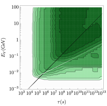
Figure 7: BBN upper limits on the product $\log_{10}(m_{V}Y_{V}/\,{\rm GeV})$ as a function of lifetime $\tau_{V}$ and injection energy $E_{V}=m_{V}/2$ for decays $V\to\gamma\gamma$ (left) and $V\to e^{+}e^{-}$ (right). The black and white lines superimposed on these plots show key thresholds for the 4P (black) and IC (white) processes discussed in the text.

Electromagnetic energy injection well above the weak scale has been shown to produce a universal photon cascade spectrum that to an excellent approximation depends only on the total amount of electromagnetic energy injected [42, 99]. Correspondingly, the limits from BBN on very massive particle decays depend on the total electromagnetic injection (and decay lifetime) but not the detailed decay type or energy spectrum. In Refs. [95, 100, 101, 102] it was shown that this feature breaks down for sub-GeV injections of photons or electrons, and thus it becomes necessary to track the type of electromagnetic injection (electrons or photons) and its energy spectrum.

In Fig. 7 we show the combined bounds from BBN on the mass times yield $m_{V}Y_{V}$ of a massive particle $V$ decaying to either $V\to\gamma\gamma$ (left) or $V\to e^{+}e^{-}$ (right) as a function of the lifetime $\tau_{V}$ and the particle injection energy $E_{V}=m_{V}/2$ from the two-body decay. This figure illustrates universality in the upper left regions of the panels with nearly identical bounds for photon and electron injection for given values of $\tau_{V}$ and $m_{V}$. However, universality is seen to break down badly in the lower right regions of the panels, with significantly different BBN bounds depending on the type of electromagnetic injection within these regions.

The breakdown of universality at lower energies can be understood in terms of the energy and temperature dependences of the photon-photon pair production (4P) and inverse Compton (IC). These two processes play a crucial role in the formation of the electromagnetic cascade, and for high-energy injection they are the dominant processes that seed the rest of the cascade and drive universality. As the injection energy falls below the weak scale, the typical interaction energy can fall below important thresholds for these reactions leading to deviations from universality.

Energetic photons injected into the cosmological plasma when the temperature is below the MeV scale interact primarily with the plasma through the 4P process. This process is very efficient relative to other processes (and the Hubble rate) provided the photon energy is greater than a critical energy $E_{c}$, given by [42, 99]

$$E_{c}=\frac{m_{e}^{2}}{22\,T}\ .$$ (70)

This corresponds to the energy threshold for $e^{+}e^{-}$ pair production on background photons extended by a Boltzmann tail. For photons with energies above the threshold $E_{c}$, the 4P process is extremely efficient and these photons are quickly reprocessed into electrons at energies below $E_{c}$. In contrast, photons with energy below $E_{c}$ are only reprocessed by other, less efficient process. The black line in Fig. 7 shows the boundary at which $E_{V}=E_{c}(\tau_{V})$, with injection energies above the 4P critical energy to the upper left of this line.

Electrons injected into the cosmological plasma below MeV temperatures with energy $E_{e}\gg T$ interact primarily through IC. This upscatters a background photon and reduces the electron energy. The energy spectrum of the upscattered photons depends sensitively on the combination [123]

$$y_{e}~{}\equiv~{}\frac{E_{e}T}{m_{e}^{2}}\ .$$ (71)

For $y_{e}\gg 1$, the scattering occurs in the Klein-Nishina regime with the outgoing photon energy $E_{\gamma}^{IC}$ typically of the same order as the initial electron energy, $E_{\gamma}^{IC}\sim E_{e}$. This allows electrons to efficiently populate the photon cascade spectrum. In contrast, when $y_{e}\ll 1$ the scattering enters the Thomson regime in which the upscattered photon energy is only a small fraction of the intial electron energy, and typically less than [123]

$$E_{\gamma}^{IC}~{}\lesssim~{}4\,T\left(\frac{E_{e}}{m_{e}}\right)^{2}\ .$$ (72)

Thus, lower-energy electrons are not able to produce photons through IC with enough energy to photodissociate light nuclei. The white line in Fig. 7 shows the threshold at which the IC photon energy produced by an electron with energy $E_{e}=E_{V}$ lies below $E_{\gamma}^{IC}\leq 2\,\,{\rm MeV}$, corresponding to the dissociation threshold for deuterium (and the lowest threshold relevant to our analysis).

Comparing the BBN exclusion contours in Fig. 7 to the 4P (black) and IC (white) threshold boundaries, we see that universality holds to a very good approximation for injection energies above these lines. Below these lines, significant deviations from universality are manifest. For photon injection with $E_{V}\sim 20$–$50\,\,{\rm MeV}<E_{c}$, the photon spectrum is more weakly suppressed and these photons are able to destroy ⁴He efficiently. As the photon injection energy falls below $E_{V}<20\,\,{\rm MeV}$, the photons are no longer able to dissociate ⁴He but can still destroy D and ³He down to near $2\,\,{\rm MeV}$. These features appear clearly in the left panel. Electron injection in the Thomson regime, corresponding to the region below the white line in the right panel, leads to much weaker limits from BBN. In this region, the dominant contribution to the photon cascade spectrum is typically hard final-state radiation (FSR) from the primary decay with a relative fraction suppressed by a factor of $\alpha$ [95].

References

- [1] E. W. Kolb and M. S. Turner, The Early Universe, Front. Phys. 69 (1990) 1–547.
- [2] S. Dodelson, Modern Cosmology. Academic Press, Amsterdam, 2003.
- [3] WMAP collaboration, G. Hinshaw et al., Nine-Year Wilkinson Microwave Anisotropy Probe (WMAP) Observations: Cosmological Parameter Results, Astrophys. J. Suppl. 208 (2013) 19, [1212.5226].
- [4] Planck collaboration, N. Aghanim et al., Planck 2018 results. VI. Cosmological parameters, 1807.06209.
- [5] SDSS collaboration, D. J. Eisenstein et al., Detection of the Baryon Acoustic Peak in the Large-Scale Correlation Function of SDSS Luminous Red Galaxies, Astrophys. J. 633 (2005) 560–574, [astro-ph/0501171].
- [6] 2dFGRS collaboration, S. Cole et al., The 2dF Galaxy Redshift Survey: Power-spectrum analysis of the final dataset and cosmological implications, Mon. Not. Roy. Astron. Soc. 362 (2005) 505–534, [astro-ph/0501174].
- [7] BOSS collaboration, S. Alam et al., The clustering of galaxies in the completed SDSS-III Baryon Oscillation Spectroscopic Survey: cosmological analysis of the DR12 galaxy sample, Mon. Not. Roy. Astron. Soc. 470 (2017) 2617–2652, [1607.03155].
- [8] Supernova Search Team collaboration, A. G. Riess et al., Observational evidence from supernovae for an accelerating universe and a cosmological constant, Astron. J. 116 (1998) 1009–1038, [astro-ph/9805201].
- [9] Supernova Cosmology Project collaboration, S. Perlmutter et al., Measurements of and from 42 high redshift supernovae, Astrophys. J. 517 (1999) 565–586, [astro-ph/9812133].
- [10] D. M. Scolnic et al., The Complete Light-curve Sample of Spectroscopically Confirmed SNe Ia from Pan-STARRS1 and Cosmological Constraints from the Combined Pantheon Sample, Astrophys. J. 859 (2018) 101, [1710.00845].
- [11] D. N. Schramm and R. V. Wagoner, Element production in the early universe, Ann. Rev. Nucl. Part. Sci. 27 (1977) 37–74.
- [12] T. P. Walker, G. Steigman, D. N. Schramm, K. A. Olive and H.-S. Kang, Primordial nucleosynthesis redux, Astrophys. J. 376 (1991) 51–69.
- [13] S. Sarkar, Big bang nucleosynthesis and physics beyond the standard model, Rept. Prog. Phys. 59 (1996) 1493–1610, [hep-ph/9602260].
- [14] F. Iocco, G. Mangano, G. Miele, O. Pisanti and P. D. Serpico, Primordial Nucleosynthesis: from precision cosmology to fundamental physics, Phys. Rept. 472 (2009) 1–76, [0809.0631].
- [15] K. Jedamzik and M. Pospelov, Big Bang Nucleosynthesis and Particle Dark Matter, New J. Phys. 11 (2009) 105028, [0906.2087].
- [16] M. Pospelov and J. Pradler, Big Bang Nucleosynthesis as a Probe of New Physics, Ann. Rev. Nucl. Part. Sci. 60 (2010) 539–568, [1011.1054].
- [17] R. H. Cyburt, B. D. Fields, K. A. Olive and T.-H. Yeh, Big Bang Nucleosynthesis: 2015, Rev. Mod. Phys. 88 (2016) 015004, [1505.01076].
- [18] B. D. Fields, K. A. Olive, T.-H. Yeh and C. Young, Big-Bang Nucleosynthesis After Planck, 1912.01132.
- [19] S. Sarkar and A. M. Cooper-Sarkar, Cosmological and experimental constraints on the tau neutrino, Phys. Lett. 148B (1984) 347–354.
- [20] R. H. Cyburt, B. D. Fields, K. A. Olive and E. Skillman, New BBN limits on physics beyond the standard model from , Astropart. Phys. 23 (2005) 313–323, [astro-ph/0408033].
- [21] C. M. Ho and R. J. Scherrer, Limits on MeV Dark Matter from the Effective Number of Neutrinos, Phys. Rev. D87 (2013) 023505, [1208.4347].
- [22] C. Boehm, M. J. Dolan and C. McCabe, A Lower Bound on the Mass of Cold Thermal Dark Matter from Planck, JCAP 1308 (2013) 041, [1303.6270].
- [23] K. M. Nollett and G. Steigman, BBN And The CMB Constrain Light, Electromagnetically Coupled WIMPs, Phys. Rev. D89 (2014) 083508, [1312.5725].
- [24] H. Ishida, M. Kusakabe and H. Okada, Effects of long-lived 10 MeV-scale sterile neutrinos on primordial elemental abundances and the effective neutrino number, Phys. Rev. D90 (2014) 083519, [1403.5995].
- [25] A. Kamada and H.-B. Yu, Coherent Propagation of PeV Neutrinos and the Dip in the Neutrino Spectrum at IceCube, Phys. Rev. D92 (2015) 113004, [1504.00711].
- [26] A. Kamada, K. Kaneta, K. Yanagi and H.-B. Yu, Self-interacting dark matter and muon in a gauged U model, JHEP 06 (2018) 117, [1805.00651].
- [27] M. Escudero, Neutrino decoupling beyond the Standard Model: CMB constraints on the Dark Matter mass with a fast and precise evaluation, JCAP 02 (2019) 007, [1812.05605].
- [28] M. Escudero, D. Hooper, G. Krnjaic and M. Pierre, Cosmology with A Very Light Gauge Boson, JHEP 03 (2019) 071, [1901.02010].
- [29] A. Berlin, N. Blinov and S. W. Li, Dark Sector Equilibration During Nucleosynthesis, Phys. Rev. D100 (2019) 015038, [1904.04256].
- [30] N. Sabti, J. Alvey, M. Escudero, M. Fairbairn and D. Blas, Refined Bounds on MeV-scale Thermal Dark Sectors from BBN and the CMB, JCAP 2001 (2020) 004, [1910.01649].
- [31] M. Kawasaki, K. Kohri and N. Sugiyama, Cosmological constraints on late time entropy production, Phys. Rev. Lett. 82 (1999) 4168, [astro-ph/9811437].
- [32] M. Kawasaki, K. Kohri and N. Sugiyama, MeV scale reheating temperature and thermalization of neutrino background, Phys. Rev. D62 (2000) 023506, [astro-ph/0002127].
- [33] S. Hannestad, What is the lowest possible reheating temperature?, Phys. Rev. D70 (2004) 043506, [astro-ph/0403291].
- [34] J. R. Ellis, D. V. Nanopoulos and S. Sarkar, The Cosmology of Decaying Gravitinos, Nucl. Phys. B259 (1985) 175–188.
- [35] R. Juszkiewicz, J. Silk and A. Stebbins, CONSTRAINTS ON COSMOLOGICALLY REGENERATED GRAVITINOS, Phys. Lett. 158B (1985) 463–467.
- [36] S. Dimopoulos, R. Esmailzadeh, L. J. Hall and G. D. Starkman, Is the Universe Closed by Baryons? Nucleosynthesis With a Late Decaying Massive Particle, Astrophys. J. 330 (1988) 545.
- [37] M. H. Reno and D. Seckel, Primordial Nucleosynthesis: The Effects of Injecting Hadrons, Phys. Rev. D37 (1988) 3441.
- [38] S. Dimopoulos, R. Esmailzadeh, L. J. Hall and G. D. Starkman, Limits on Late Decaying Particles From Nucleosynthesis, Nucl. Phys. B311 (1989) 699–718.
- [39] J. R. Ellis, G. B. Gelmini, J. L. Lopez, D. V. Nanopoulos and S. Sarkar, Astrophysical constraints on massive unstable neutral relic particles, Nucl. Phys. B373 (1992) 399–437.
- [40] T. Moroi, H. Murayama and M. Yamaguchi, Cosmological constraints on the light stable gravitino, Phys. Lett. B303 (1993) 289–294.
- [41] M. Kawasaki and T. Moroi, Gravitino production in the inflationary universe and the effects on big bang nucleosynthesis, Prog. Theor. Phys. 93 (1995) 879–900, [hep-ph/9403364].
- [42] R. H. Cyburt, J. R. Ellis, B. D. Fields and K. A. Olive, Updated nucleosynthesis constraints on unstable relic particles, Phys. Rev. D67 (2003) 103521, [astro-ph/0211258].
- [43] K. Jedamzik, Did something decay, evaporate, or annihilate during Big Bang nucleosynthesis?, Phys. Rev. D70 (2004) 063524, [astro-ph/0402344].
- [44] M. Kawasaki, K. Kohri and T. Moroi, Big-Bang nucleosynthesis and hadronic decay of long-lived massive particles, Phys. Rev. D71 (2005) 083502, [astro-ph/0408426].
- [45] K. Jedamzik, Big bang nucleosynthesis constraints on hadronically and electromagnetically decaying relic neutral particles, Phys. Rev. D74 (2006) 103509, [hep-ph/0604251].
- [46] M. Kawasaki, K. Kohri, T. Moroi and A. Yotsuyanagi, Big-Bang Nucleosynthesis and Gravitino, Phys. Rev. D78 (2008) 065011, [0804.3745].
- [47] M. Kawasaki, K. Kohri, T. Moroi and Y. Takaesu, Revisiting Big-Bang Nucleosynthesis Constraints on Long-Lived Decaying Particles, Phys. Rev. D97 (2018) 023502, [1709.01211].
- [48] J. A. Frieman, E. W. Kolb and M. S. Turner, Eternal Annihilations: New Constraints on Longlived Particles from Big Bang Nucleosynthesis, Phys. Rev. D41 (1990) 3080.
- [49] J. Hisano, M. Kawasaki, K. Kohri and K. Nakayama, Positron/Gamma-Ray Signatures of Dark Matter Annihilation and Big-Bang Nucleosynthesis, Phys. Rev. D79 (2009) 063514, [0810.1892].
- [50] J. Hisano, M. Kawasaki, K. Kohri, T. Moroi and K. Nakayama, Cosmic Rays from Dark Matter Annihilation and Big-Bang Nucleosynthesis, Phys. Rev. D79 (2009) 083522, [0901.3582].
- [51] M. Kawasaki, K. Kohri, T. Moroi and Y. Takaesu, Revisiting Big-Bang Nucleosynthesis Constraints on Dark-Matter Annihilation, Phys. Lett. B751 (2015) 246–250, [1509.03665].
- [52] P. F. Depta, M. Hufnagel, K. Schmidt-Hoberg and S. Wild, BBN constraints on the annihilation of MeV-scale dark matter, JCAP 1904 (2019) 029, [1901.06944].
- [53] W. Hu and J. Silk, Thermalization and spectral distortions of the cosmic background radiation, Phys. Rev. D48 (1993) 485–502.
- [54] W. Hu and J. Silk, Thermalization constraints and spectral distortions for massive unstable relic particles, Phys. Rev. Lett. 70 (1993) 2661–2664.
- [55] J. A. Adams, S. Sarkar and D. W. Sciama, CMB anisotropy in the decaying neutrino cosmology, Mon. Not. Roy. Astron. Soc. 301 (1998) 210–214, [astro-ph/9805108].
- [56] X.-L. Chen and M. Kamionkowski, Particle decays during the cosmic dark ages, Phys. Rev. D70 (2004) 043502, [astro-ph/0310473].
- [57] N. Padmanabhan and D. P. Finkbeiner, Detecting dark matter annihilation with CMB polarization: Signatures and experimental prospects, Phys. Rev. D72 (2005) 023508, [astro-ph/0503486].
- [58] L. Zhang, X. Chen, M. Kamionkowski, Z.-g. Si and Z. Zheng, Constraints on radiative dark-matter decay from the cosmic microwave background, Phys. Rev. D76 (2007) 061301, [0704.2444].
- [59] T. R. Slatyer, N. Padmanabhan and D. P. Finkbeiner, CMB Constraints on WIMP Annihilation: Energy Absorption During the Recombination Epoch, Phys. Rev. D80 (2009) 043526, [0906.1197].
- [60] G. Huetsi, A. Hektor and M. Raidal, Constraints on leptonically annihilating Dark Matter from reionization and extragalactic gamma background, Astron. Astrophys. 505 (2009) 999–1005, [0906.4550].
- [61] G. Hutsi, J. Chluba, A. Hektor and M. Raidal, WMAP7 and future CMB constraints on annihilating dark matter: implications on GeV-scale WIMPs, Astron. Astrophys. 535 (2011) A26, [1103.2766].
- [62] M. Dutra, M. Lindner, S. Profumo, F. S. Queiroz, W. Rodejohann and C. Siqueira, MeV Dark Matter Complementarity and the Dark Photon Portal, JCAP 03 (2018) 037, [1801.05447].
- [63] R. Slansky, Group Theory for Unified Model Building, Phys. Rept. 79 (1981) 1–128.
- [64] J. L. Hewett and T. G. Rizzo, Low-Energy Phenomenology of Superstring Inspired E(6) Models, Phys. Rept. 183 (1989) 193.
- [65] A. Leike, The Phenomenology of extra neutral gauge bosons, Phys. Rept. 317 (1999) 143–250, [hep-ph/9805494].
- [66] R. Blumenhagen, M. Cvetic, P. Langacker and G. Shiu, Toward realistic intersecting D-brane models, Ann. Rev. Nucl. Part. Sci. 55 (2005) 71–139, [hep-th/0502005].
- [67] M. R. Douglas and S. Kachru, Flux compactification, Rev. Mod. Phys. 79 (2007) 733–796, [hep-th/0610102].
- [68] R. Blumenhagen, B. Kors, D. Lust and S. Stieberger, Four-dimensional String Compactifications with D-Branes, Orientifolds and Fluxes, Phys. Rept. 445 (2007) 1–193, [hep-th/0610327].
- [69] P. Fayet, U-boson production in e+ e- annihilations, psi and Upsilon decays, and Light Dark Matter, Phys. Rev. D75 (2007) 115017, [hep-ph/0702176].
- [70] M. Pospelov, A. Ritz and M. B. Voloshin, Secluded WIMP Dark Matter, Phys. Lett. B662 (2008) 53–61, [0711.4866].
- [71] N. Arkani-Hamed, D. P. Finkbeiner, T. R. Slatyer and N. Weiner, A Theory of Dark Matter, Phys. Rev. D79 (2009) 015014, [0810.0713].
- [72] M. Pospelov, Secluded U(1) below the weak scale, Phys. Rev. D80 (2009) 095002, [0811.1030].
- [73] J. D. Bjorken, R. Essig, P. Schuster and N. Toro, New Fixed-Target Experiments to Search for Dark Gauge Forces, Phys. Rev. D80 (2009) 075018, [0906.0580].
- [74] J. Alexander et al., Dark Sectors 2016 Workshop: Community Report, 2016. 1608.08632.
- [75] Z. G. Berezhiani, A. D. Dolgov and R. N. Mohapatra, Asymmetric inflationary reheating and the nature of mirror universe, Phys. Lett. B375 (1996) 26–36, [hep-ph/9511221].
- [76] P. Adshead, Y. Cui and J. Shelton, Chilly Dark Sectors and Asymmetric Reheating, JHEP 06 (2016) 016, [1604.02458].
- [77] E. Hardy and J. Unwin, Symmetric and Asymmetric Reheating, JHEP 09 (2017) 113, [1703.07642].
- [78] P. Adshead, P. Ralegankar and J. Shelton, Reheating in two-sector cosmology, JHEP 08 (2019) 151, [1906.02755].
- [79] L. J. Hall, K. Jedamzik, J. March-Russell and S. M. West, Freeze-In Production of FIMP Dark Matter, JHEP 03 (2010) 080, [0911.1120].
- [80] C. Cheung, G. Elor, L. J. Hall and P. Kumar, Origins of Hidden Sector Dark Matter I: Cosmology, JHEP 03 (2011) 042, [1010.0022].
- [81] X. Chu, T. Hambye and M. H. G. Tytgat, The Four Basic Ways of Creating Dark Matter Through a Portal, JCAP 1205 (2012) 034, [1112.0493].
- [82] X. Chu, Y. Mambrini, J. Quevillon and B. Zaldivar, Thermal and non-thermal production of dark matter via Z’-portal(s), JCAP 1401 (2014) 034, [1306.4677].
- [83] N. Bernal, M. Heikinheimo, T. Tenkanen, K. Tuominen and V. Vaskonen, The Dawn of FIMP Dark Matter: A Review of Models and Constraints, Int. J. Mod. Phys. A32 (2017) 1730023, [1706.07442].
- [84] D. Hooper, N. Weiner and W. Xue, Dark Forces and Light Dark Matter, Phys. Rev. D86 (2012) 056009, [1206.2929].
- [85] J. Hasenkamp and J. Kersten, Dark radiation from particle decay: cosmological constraints and opportunities, JCAP 1308 (2013) 024, [1212.4160].
- [86] A. Fradette, M. Pospelov, J. Pradler and A. Ritz, Cosmological Constraints on Very Dark Photons, Phys. Rev. D90 (2014) 035022, [1407.0993].
- [87] J. Berger, K. Jedamzik and D. G. E. Walker, Cosmological Constraints on Decoupled Dark Photons and Dark Higgs, JCAP 1611 (2016) 032, [1605.07195].
- [88] L. B. Okun, LIMITS OF ELECTRODYNAMICS: PARAPHOTONS?, Sov. Phys. JETP 56 (1982) 502.
- [89] B. Holdom, Two U(1)’s and Epsilon Charge Shifts, Phys. Lett. 166B (1986) 196–198.
- [90] J. Heeck, Unbroken B – L symmetry, Phys. Lett. B739 (2014) 256–262, [1408.6845].
- [91] Y. S. Jeong, C. S. Kim and H.-S. Lee, Constraints on the gauge boson in a wide mass range, Int. J. Mod. Phys. A31 (2016) 1650059, [1512.03179].
- [92] M. B. Wise and Y. Zhang, Lepton Flavorful Fifth Force and Depth-dependent Neutrino Matter Interactions, JHEP 06 (2018) 053, [1803.00591].
- [93] W. Altmannshofer, S. Gori, M. Pospelov and I. Yavin, Neutrino Trident Production: A Powerful Probe of New Physics with Neutrino Beams, Phys. Rev. Lett. 113 (2014) 091801, [1406.2332].
- [94] Y. Kaneta and T. Shimomura, On the possibility of a search for the gauge boson at Belle-II and neutrino beam experiments, PTEP 2017 (2017) 053B04, [1701.00156].
- [95] L. Forestell, D. E. Morrissey and G. White, Limits from BBN on Light Electromagnetic Decays, JHEP 01 (2019) 074, [1809.01179].
- [96] F. A. Aharonian, A. M. Atoian and A. M. Nagapetian, Photoproduction of electron-positron pairs in compact X-ray sources, Astrofizika 19 (Apr., 1983) 323–334.
- [97] R. Svensson and A. A. Zdziarski, Photon-photon scattering of gamma rays at cosmological distances, Astrophys. J. 349 (1990) 415–428.
- [98] R. J. Protheroe, T. Stanev and V. S. Berezinsky, Electromagnetic cascades and cascade nucleosynthesis in the early universe, Phys. Rev. D51 (1995) 4134–4144, [astro-ph/9409004].
- [99] M. Kawasaki and T. Moroi, Electromagnetic cascade in the early universe and its application to the big bang nucleosynthesis, Astrophys. J. 452 (1995) 506, [astro-ph/9412055].
- [100] V. Poulin and P. D. Serpico, Loophole to the Universal Photon Spectrum in Electromagnetic Cascades and Application to the Cosmological Lithium Problem, Phys. Rev. Lett. 114 (2015) 091101, [1502.01250].
- [101] V. Poulin and P. D. Serpico, Nonuniversal BBN bounds on electromagnetically decaying particles, Phys. Rev. D91 (2015) 103007, [1503.04852].
- [102] M. Hufnagel, K. Schmidt-Hoberg and S. Wild, BBN constraints on MeV-scale dark sectors. Part II. Electromagnetic decays, 1808.09324.
- [103] A. Coogan, L. Morrison and S. Profumo, Hazma: A Python Toolkit for Studying Indirect Detection of Sub-GeV Dark Matter, 1907.11846.
- [104] T. Plehn, P. Reimitz and P. Richardson, Hadronic Footprint of GeV-Mass Dark Matter, 1911.11147.
- [105] P. Ilten, Y. Soreq, M. Williams and W. Xue, Serendipity in dark photon searches, JHEP 06 (2018) 004, [1801.04847].
- [106] M. Bauer, P. Foldenauer and J. Jaeckel, Hunting All the Hidden Photons, JHEP 07 (2018) 094, [1803.05466].
- [107] R. M. Schabinger and J. D. Wells, A Minimal spontaneously broken hidden sector and its impact on Higgs boson physics at the large hadron collider, Phys. Rev. D72 (2005) 093007, [hep-ph/0509209].
- [108] E. C. G. Stueckelberg, Interaction energy in electrodynamics and in the field theory of nuclear forces, Helv. Phys. Acta 11 (1938) 225–244.
- [109] D. Feldman, Z. Liu and P. Nath, The Stueckelberg Z-prime Extension with Kinetic Mixing and Milli-Charged Dark Matter From the Hidden Sector, Phys. Rev. D75 (2007) 115001, [hep-ph/0702123].
- [110] S. Tulin, New weakly-coupled forces hidden in low-energy QCD, Phys. Rev. D89 (2014) 114008, [1404.4370].
- [111] J. J. Sakurai, Theory of strong interactions, Annals Phys. 11 (1960) 1–48.
- [112] T. Fujiwara, T. Kugo, H. Terao, S. Uehara and K. Yamawaki, Nonabelian Anomaly and Vector Mesons as Dynamical Gauge Bosons of Hidden Local Symmetries, Prog. Theor. Phys. 73 (1985) 926.
- [113] M. Bando, T. Kugo, S. Uehara, K. Yamawaki and T. Yanagida, Is rho Meson a Dynamical Gauge Boson of Hidden Local Symmetry?, Phys. Rev. Lett. 54 (1985) 1215.
- [114] H. B. O’Connell, B. C. Pearce, A. W. Thomas and A. G. Williams, mixing, vector meson dominance and the pion form-factor, Prog. Part. Nucl. Phys. 39 (1997) 201–252, [hep-ph/9501251].
- [115] BaBar collaboration, J. P. Lees et al., Precise Measurement of the Cross Section with the Initial-State Radiation Method at BABAR, Phys. Rev. D86 (2012) 032013, [1205.2228].
- [116] J. Bellm et al., Herwig 7.0/Herwig++ 3.0 release note, Eur. Phys. J. C76 (2016) 196, [1512.01178].
- [117] L. Michel, Interaction between four half spin particles and the decay of the meson, Proc. Phys. Soc. A63 (1950) 514–531.
- [118] Particle Data Group collaboration, M. Tanabashi et al., Review of Particle Physics, Phys. Rev. D98 (2018) 030001.
- [119] A. Scaffidi, K. Freese, J. Li, C. Savage, M. White and A. G. Williams, Gamma rays from muons from WIMPs: Implementation of radiative muon decays for dark matter analyses, Phys. Rev. D93 (2016) 115024, [1604.00744].
- [120] Y. Kuno and Y. Okada, Muon decay and physics beyond the standard model, Rev. Mod. Phys. 73 (2001) 151–202, [hep-ph/9909265].
- [121] PiENu collaboration, A. Aguilar-Arevalo et al., Improved Measurement of the Branching Ratio, Phys. Rev. Lett. 115 (2015) 071801, [1506.05845].
- [122] M. Pospelov and J. Pradler, Metastable GeV-scale particles as a solution to the cosmological lithium problem, Phys. Rev. D82 (2010) 103514, [1006.4172].
- [123] G. R. Blumenthal and R. J. Gould, Bremsstrahlung, synchrotron radiation, and compton scattering of high-energy electrons traversing dilute gases, Rev. Mod. Phys. 42 (1970) 237–270.
- [124] O. Pisanti, A. Cirillo, S. Esposito, F. Iocco, G. Mangano, G. Miele et al., PArthENoPE: Public Algorithm Evaluating the Nucleosynthesis of Primordial Elements, Comput. Phys. Commun. 178 (2008) 956–971, [0705.0290].
- [125] R. Consiglio, P. F. de Salas, G. Mangano, G. Miele, S. Pastor and O. Pisanti, PArthENoPE reloaded, Comput. Phys. Commun. 233 (2018) 237–242, [1712.04378].
- [126] E. Aver, K. A. Olive and E. D. Skillman, The effects of He I 10830 on helium abundance determinations, JCAP 1507 (2015) 011, [1503.08146].
- [127] R. J. Cooke, M. Pettini and C. C. Steidel, One Percent Determination of the Primordial Deuterium Abundance, Astrophys. J. 855 (2018) 102, [1710.11129].
- [128] J. Geiss and G. Gloeckler, Isotopic Composition of H, HE and NE in the Protosolar Cloud, Space Science Reviews 106 (2003) 3–18.
- [129] A. Peimbert, M. Peimbert and V. Luridiana, The primordial helium abundance and the number of neutrino families, Rev. Mex. Astron. Astrofis. 52 (2016) 419, [1608.02062].
- [130] Y. I. Izotov, T. X. Thuan and N. G. Guseva, A new determination of the primordial He abundance using the He i 10830 A emission line: cosmological implications, Mon. Not. Roy. Astron. Soc. 445 (2014) 778–793, [1408.6953].
- [131] L. E. Marcucci, G. Mangano, A. Kievsky and M. Viviani, Implication of the proton-deuteron radiative capture for Big Bang Nucleosynthesis, Phys. Rev. Lett. 116 (2016) 102501, [1510.07877].
- [132] M. Ibe, S. Kobayashi, Y. Nakayama and S. Shirai, Cosmological Constraint on Dark Photon from , 1912.12152.
- [133] V. Barger, P. Langacker and H.-S. Lee, Primordial nucleosynthesis constraints on properties, Phys. Rev. D67 (2003) 075009, [hep-ph/0302066].
- [134] T. R. Slatyer, Energy Injection And Absorption In The Cosmic Dark Ages, Phys. Rev. D87 (2013) 123513, [1211.0283].
- [135] V. Poulin, J. Lesgourgues and P. D. Serpico, Cosmological constraints on exotic injection of electromagnetic energy, JCAP 1703 (2017) 043, [1610.10051].
- [136] T. R. Slatyer, Indirect Dark Matter Signatures in the Cosmic Dark Ages II. Ionization, Heating and Photon Production from Arbitrary Energy Injections, Phys. Rev. D93 (2016) 023521, [1506.03812].
- [137] T. R. Slatyer, Energy Injection And Absorption In The Cosmic Dark Ages, https://faun.rc.fas.harvard.edu/epsilon/, 2012.
- [138] S. Galli, T. R. Slatyer, M. Valdes and F. Iocco, Systematic Uncertainties In Constraining Dark Matter Annihilation From The Cosmic Microwave Background, Phys. Rev. D88 (2013) 063502, [1306.0563].
- [139] D. P. Finkbeiner, S. Galli, T. Lin and T. R. Slatyer, Searching for Dark Matter in the CMB: A Compact Parameterization of Energy Injection from New Physics, Phys. Rev. D85 (2012) 043522, [1109.6322].
- [140] J. Lesgourgues, The Cosmic Linear Anisotropy Solving System (CLASS) I: Overview, 1104.2932.
- [141] A. Lewis and S. Bridle, Cosmological parameters from CMB and other data: A Monte Carlo approach, Phys. Rev. D66 (2002) 103511, [astro-ph/0205436].
- [142] J. M. Cline and P. Scott, Dark Matter CMB Constraints and Likelihoods for Poor Particle Physicists, JCAP 1303 (2013) 044, [1301.5908].
- [143] J. M. Shull and M. E. van Steenberg, X-ray secondary heating and ionization in quasar emission-line clouds, Astrophys. J. 298 (1985) 268.
- [144] M. S. Madhavacheril, N. Sehgal and T. R. Slatyer, Current Dark Matter Annihilation Constraints from CMB and Low-Redshift Data, Phys. Rev. D89 (2014) 103508, [1310.3815].
- [145] T. R. Slatyer, Indirect dark matter signatures in the cosmic dark ages. I. Generalizing the bound on s-wave dark matter annihilation from Planck results, Phys. Rev. D93 (2016) 023527, [1506.03811].
- [146] T. R. Slatyer and C.-L. Wu, General Constraints on Dark Matter Decay from the Cosmic Microwave Background, Phys. Rev. D95 (2017) 023010, [1610.06933].
- [147] Planck collaboration, P. A. R. Ade et al., Planck 2015 results. XIII. Cosmological parameters, Astron. Astrophys. 594 (2016) A13, [1502.01589].
- [148] D. J. Fixsen, E. S. Cheng, J. M. Gales, J. C. Mather, R. A. Shafer and E. L. Wright, The Cosmic Microwave Background spectrum from the full COBE FIRAS data set, Astrophys. J. 473 (1996) 576, [astro-ph/9605054].
- [149] A. Kogut et al., The Primordial Inflation Explorer (PIXIE): A Nulling Polarimeter for Cosmic Microwave Background Observations, JCAP 1107 (2011) 025, [1105.2044].
- [150] J. Chluba and R. A. Sunyaev, The evolution of CMB spectral distortions in the early Universe, Mon. Not. Roy. Astron. Soc. 419 (2012) 1294–1314, [1109.6552].
- [151] J. Chluba, Green’s function of the cosmological thermalization problem, Mon. Not. Roy. Astron. Soc. 434 (2013) 352, [1304.6120].
- [152] J. Chluba and D. Jeong, Teasing bits of information out of the CMB energy spectrum, Mon. Not. Roy. Astron. Soc. 438 (2014) 2065–2082, [1306.5751].
- [153] J. Chluba, Which spectral distortions does CDM actually predict?, Mon. Not. Roy. Astron. Soc. 460 (2016) 227–239, [1603.02496].
- [154] P. Gondolo and G. Gelmini, Cosmic abundances of stable particles: Improved analysis, Nucl. Phys. B360 (1991) 145–179.
- [155] J. Edsjo and P. Gondolo, Neutralino relic density including coannihilations, Phys. Rev. D56 (1997) 1879–1894, [hep-ph/9704361].
- [156] D. Kazanas, R. N. Mohapatra, S. Nussinov, V. L. Teplitz and Y. Zhang, Supernova Bounds on the Dark Photon Using its Electromagnetic Decay, Nucl. Phys. B890 (2014) 17–29, [1410.0221].
- [157] W. DeRocco, P. W. Graham, D. Kasen, G. Marques-Tavares and S. Rajendran, Observable signatures of dark photons from supernovae, JHEP 02 (2019) 171, [1901.08596].
- [158] R. Essig, E. Kuflik, S. D. McDermott, T. Volansky and K. M. Zurek, Constraining Light Dark Matter with Diffuse X-Ray and Gamma-Ray Observations, JHEP 11 (2013) 193, [1309.4091].
- [159] T. Gherghetta, J. Kersten, K. Olive and M. Pospelov, Evaluating the price of tiny kinetic mixing, Phys. Rev. D100 (2019) 095001, [1909.00696].
- [160] A. DiFranzo, P. J. Fox and T. M. P. Tait, Vector Dark Matter through a Radiative Higgs Portal, JHEP 04 (2016) 135, [1512.06853].
- [161] S. Koren and R. McGehee, Freezing-in twin dark matter, Phys. Rev. D101 (2020) 055024, [1908.03559].
- [162] C. Vafa, The String landscape and the swampland, hep-th/0509212.
- [163] N. Arkani-Hamed, L. Motl, A. Nicolis and C. Vafa, The String landscape, black holes and gravity as the weakest force, JHEP 06 (2007) 060, [hep-th/0601001].
- [164] H. Ooguri and C. Vafa, On the Geometry of the String Landscape and the Swampland, Nucl. Phys. B766 (2007) 21–33, [hep-th/0605264].