A mathematical model of platelet aggregation in an extravascular injury under flow.

Abstract

We present the first mathematical model of flow-mediated primary hemostasis in an extravascular injury which can track the process from initial deposition to occlusion. The model consists of a system of ordinary differential equations (ODE) that describe platelet aggregation (adhesion and cohesion), soluble-agonist-dependent platelet activation, and the flow of blood through the injury. The formation of platelet aggregates increases resistance to flow through the injury, which is modeled using the Stokes-Brinkman equations. Data from analogous experimental (microfluidic flow) and partial differential equation models informed parameter values used in the ODE model description of platelet adhesion, cohesion, and activation. This model predicts injury occlusion under a range of flow and platelet activation conditions. Simulations testing the effects of shear and activation rates resulted in delayed occlusion and aggregate heterogeneity. These results validate our hypothesis that flow-mediated dilution of activating chemical ADP hinders aggregate development. This novel modeling framework can be extended to include more mechanisms of platelet activation as well as the addition of the biochemical reactions of coagulation, resulting in a computationally efficient high throughput screening tool.

92B05, 76S99, 93A30

1 Introduction

Hemostasis is the first line of defense upon vascular injury (either a disruption in the subendothelial lining or a breach in the vessel wall) whereby a blood clot (thrombus) forms to prevent the loss of blood [47, 48]. The hemostatic response consists of two intertwined processes: platelet aggregate formation and coagulation [13, 34]. These processes are triggered when reactive proteins either in the extravascular matrix or on the subendothelium are exposed to the blood plasma. Platelets are blood cells that circulate in the human vasculature in their unactivated state and mediate the biophysical and biochemical aspects of thrombus formation. Platelets become activated when in contact with collagen in the subendothelium or with chemical agonists in the plasma. Activated platelet surfaces support coagulation reactions that produce the enzyme thrombin. Thrombin in turn cleaves the soluble blood protein fibrinogen into fibrin monomers, which polymerize to form a gel. This gel provides structure and stability to the aggregate. The size and structure of an aggregate as well as the time it takes the aggregate to form, depend not only on platelet function and coagulation, but on the local hydrodynamic environment. Blood flowing in a vessel is subject to a pressure difference across the vascular wall and any disruption of the wall can lead to loss of blood, which greatly affects the delivery and removal of platelets, chemical agonists, and coagulation proteins.

Upon extravascular injury, two important reactive proteins are exposed: collagen and tissue factor (TF). Blood cells and plasma containing coagulation proteins leak from the vessel into the extravascular space. Platelets flow into the injury and begin to deposit; they adhere to the collagen, and bind other insoluble agonists, which in turn triggers the activation of key integrins on platelet surfaces [2, 4, 14, 21, 48]. The soluble agonist ADP, which is released from platelet granules into the fluid by activated platelets themselves, interacts with platelet receptors P2Y₁ and P2Y₁₂ to additionally trigger exposure of surface integrins [3, 18, 33]. This effect of soluble agonist ADP is an example of activation without contact with the subendothelial matrix [1, 27]. Activated platelets provide surfaces to which more platelets can cohere, enhancing to the growth of the platelet aggregate to prevent further blood leakage. Platelet aggregate formation depends strongly on both the hydrodynamic environment and the formation and dissociation of bonds that enable platelet adhesion and cohesion. Failure of any of the processes that mediate platelet aggregation, under a variety of flow conditions, can result in significant blood loss.

In recent years there has been an increased focus on understanding the molecular basis of bleeding disorders and associated variability in levels of key coagulation factors, platelet count, and insoluble proteins. Most clinical assays used to assess bleeding risk are performed under static conditions. However, data has shown that hydrodynamic forces affect platelet aggregation and fibrin formation, both key components of a thrombus [31]. This has motivated the development of mathematical models of hemostasis that integrate platelet function, coagulation, and hemodynamics to predict bleeding risk based on measurable biochemical and biophysical factors.

Our group has developed mathematical models of flow-mediated coagulation in an intravascular injury setting to predict regulatory mechanisms of hemostasis and thrombosis [10, 12, 15, 22, 23, 24, 25, 28, 29]. These models use a continuum approach and express dynamics using differential equations. Our ordinary differential equation (ODE) models of thrombosis employ a well-mixed compartment assumption that accounts for transport by flow and diffusion using simplified mass-transfer coefficients. Other models fully account for spatial variations and transport to simulate small vascular injuries under flow [24, 26] through the use of partial differential equations (PDEs). Despite the numerous mathematical models of flow-mediated intravascular blood clotting, there are relatively few models of hemostasis. To our knowledge, the model we present here is the first mathematical model to incorporate key biophysical and biochemical mechanisms of primary hemostasis in the framework of an extravascular injury. Our model is based on ODEs and is calibrated and validated using analogous experimental (Section A.2) and PDE (Section A.4) models [7, 40].

One of the many contributions of this model is its computational efficiency, which allows for systematic exploration of large sets of parameters that would be impossible to resolve using the spatial PDE model or an experimental model. Parameters that contribute to bleeding include, but are not limited to, injury size, hemodynamics, vessel wall composition, and the anatomy of the adjacent perivascular and extravascular spaces. An experimental platform for studying hemostasis with a focus on collagen-TF induced thrombus formation within a model vascular wall was previously presented in [40]. This experimental model is an in vitro microfluidic flow assay (MFA) we refer to as the “bleeding chip”. Our mathematical model design is inspired by the specific ‘H’-geometry that is characteristic of the bleeding chip and will be used in the future to quantify variability of MFAs and identify components of the clotting system that underscore the known phenotypic variability in certain bleeding disorders [32]. The goal of this work is to create an efficient, mechanistic model that can be used for high-throughput screening of the blood clotting process and that enables mathematically-driven, but testable hypotheses.

The paper is organized as follows. In Section 2, we present a system of ordinary differential equations that describe platelet accumulation, soluble agonist-dependent platelet activation, and flow through the injury. Flow and aggregate calculations are calibrated using occlusion times and flow rates from the bleeding chip shown in Section 3. Also in Section 3 are simulations to test the effects of flow and platelet activation rates on occlusion times. The results therein suggest that inhibition of platelet activation significantly modifies primary hemostasis. Additionally, flow-mediated dilution of ADP is shown to hinder aggregate development, as discussed in Section 4.

(A)                                                        (B)

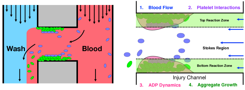
Figure 1: (A) Bleeding chip. Blood and wash buffer are introduced into the two vertical channels of the bleeding chip. A horizontal injury channel connects the two vertical channels, where platelet deposition occurs [40]. (B) Mathematical model components. 1. Pressure driven flow with a Stokes-Brinkman layered velocity calculation. 2. Platelets’ state (mobile/bound and unactivated/activated), mediated by activating chemical concentration [ADP], determines adhesion to injury and cohesion to other platelets. (3) ADP is released from bound platelets and is subject to transport by both advection and diffusion. (4) Aggregate growth is influenced by changes in thickness and porosity and feedbacks on blood flow due to increased frictional resistance.

2 Mathematical Model

We model the situation where blood flows through a hole in the vessel wall into the extravascular space. In this scenario, a disruption in the endothelial layer occurs and exposes collagen to the blood. Platelets are transported to the injury by flow and adhere to collagen. This in turn activates them, leading to the release of platelet agonist ADP and the recruitment of additional platelets that cohere and form an aggregate. The model incorporates the flow of blood through an ‘H’-geometry to mimic the bleeding chip, as described above and as depicted in Fig. 1A, and it explicitly models aggregate formation under local fluid dynamic conditions. Components of the model include descriptions of the blood flow through the bleeding chip geometry and the injury channel as well as the platelet interactions, soluble agonist ADP dynamics, and aggregate growth (see Fig. 1B).

(A)                                (B)                                (C)

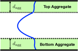
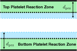
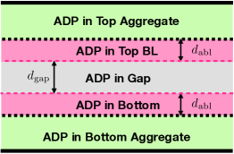
Figure 2: Spatial compartments of model. Each panel shows spatial compartments of the injury channel. (A) Two aggregate (Brinkman) compartments with thickness $d_{\text{agg}}$ with a volume of $V_{\text{agg}}$ and the Stokes region. (B) Two aggregate compartments and the platelet boundary layers (PBL), together defining platelet reaction zones (PRZ) with thicknesses of $d_{\text{prz}}$ and volumes $V_{\text{prz}}$ describe a two compartment platelet model. (C) Two aggregate compartments and the boundary layers associated with ADP (ABL) with thicknesses $d_{\text{abl}}$. The remaining compartment in the bulk of the Stokes region is denoted as the “gap” and has thickness $d_{\text{gap}}$. These layers define a five compartment ADP model.

Each component of the model involves a number of compartments which correspond to different spatial portions of the injury channel. Two compartments are defined by the platelet aggregates on the bottom and top walls of the channel as shown in Fig. 2A. Others are defined in terms of diffusive boundary layers for platelets (Fig. 2B) and the activating chemical ADP (Fig. 2C). There are diffusive boundary layers associated with each of the aggregates. Lastly, there is a compartment representing the ‘gap’ between the boundary layers associated with the bottom and top aggregates shown in Fig. 2C. The two compartments of the platelet model and the five compartments describing the ADP model are defined precisely below. The model unknowns are number densities for three populations of platelets and the concentration of ADP in the various compartments; the volume fraction of bound platelets in and the thickness of each of the aggregate compartments, and the fluid velocity profile across the channel. The velocity profile is the only fully spatially-dependent variable in the model; it is used in defining the diffusive boundary layers and in defining advective fluxes of fluid, platelets, and ADP into and out of the various compartments.

2.1 Fluid Dynamics

The mathematical representation of flow in this geometry is nonstandard. Below, we describe how we model pressure-driven flow in the injury channel and incorporate hinderance by the porous, growing aggregate. The flow of blood through the bleeding chip is described in Section 2.1.1. Output from this calculation determines the inputs used in the Stokes-Brinkman calculation of the flow inside of the injury channel where aggregates form. The resulting velocity profile is used to calculate the increased resistance in the injury channel and therefore alters the pressure drop $P_{1}-P_{2}$. Details of this calculation are found in Section 2.1.2.

(A)	(B)

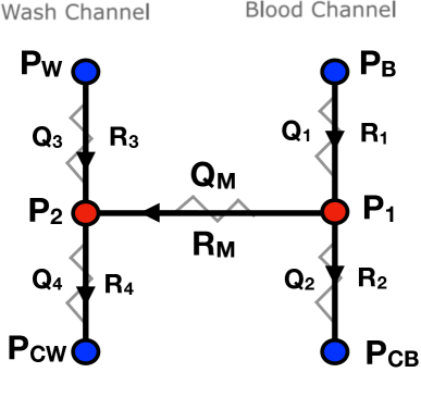
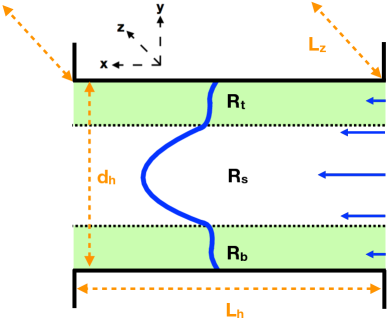
Figure 3: (A) Hydraulic circuit (HC) system describing flow through the bleeding chip. Quantities in blue are inputs while quantities in red are the desired output determined by solving system of equations in Section A.1. (B) A schematic of the domain filled with Brinkman regions green representing the bottom $R_{b}$ and top aggregates $R_{\text{t}}$ and a Stokes region $R_{\text{s}}$ with a depth of $L_{z}$, width of $d_{h}$, and a length of $L_{z}$ denoted in orange. Flow moves from right to left and the resulting velocity profile is depicted in blue.

2.1.1 Fluid through Extravascular Injury Domain

The bleeding chip contains two vertical channels $(L\times w\times L_{z})=(10\ \text{mm}\ \times\ 100\ \mu\text{m}\ \times 60\ \mu\text{m})$, consisting of a ‘blood’ channel and a ‘wash’ channel, connected by a horizontal ‘injury’ channel $(L_{h}\times d_{h}\times L_{z})=(150\ \mu\text{m}\ \times\ 20\ \mu\text{m}\ \times 60\ \mu\text{m})$, which forms an ‘H’-shaped geometry (Fig. 1A). The flow rates and/or pressures at the inlets and outlets are prescribed and blood flows into the device through the blood channel. A fraction of the blood exits through the outlet of the blood channel. The remaining blood makes its way through the injury channel (from right to left) and exits through the outlet of the injury channel into the wash channel. Two hydraulic resistors in series describe the flow in each of the blood and wash channels and a connecting resistor in parallel describes the flow in the injury channel (Fig. 3A). The resistances $R_{1}$, $R_{2}$, $R_{3}$, $R_{4}$ are input parameters; the resistance $R_{M}$ is obtained from our calculation of the flow in the injury channel as explained in the next section. By solving the linear system of equations for this hydraulic circuit (HC) as shown in Section A.1, we determine the pressure gradient $G_{h}=(P_{1}-P_{2})/L_{h}$ across the injury channel. The resulting pressure gradient $G_{h}$ is used to determine the flow velocity through the injury channel.

2.1.2 Fluid through Injury

The calculation of the fluid velocity profile at each time proceeds as follows. We assume that we know the current thicknesses $d_{\text{b}}$ and $d_{\text{t}}$ of the aggregate compartments (see Fig. 2A), and the volume fractions of bound platelets $\theta_{\text{b}}^{B}$ and $\theta_{\text{t}}^{B}$ of the aggregates. Define the intervals $R_{\text{b}}=\{0\leq y\leq d_{\text{b}}\}$, $R_{\text{s}}=\{d_{\text{b}}\leq y\leq d_{\text{h}}-d_{\text{t}}\}$, and $R_{\text{t}}=\{d_{\text{h}}-d_{\text{t}}\leq y\leq d_{\text{h}}\}$. Given that the Reynolds number in the injury channel of the bleeding chip is $R_{e}\approx 0.0283<<1$ as calculated in Table 4, the unidirectional flow in the $x$-direction for $y\in R_{\text{s}}$ is modeled by the Stokes equations, and the flows for $y\in R_{\text{b}}$ and $y\in R_{\text{t}}$ are modeled by the Brinkman equations, as we have done in previous studies [23, 24]. These are the Stokes equations modified by the inclusion of a Brinkman drag term among the forces acting on the fluid. The fluid dynamics equations are

(1) $$0=-\frac{\partial p_{\text{b}}}{\partial x}+\mu\frac{\partial^{2}u_{\text{b}}}{\partial y^{2}}-\mu\alpha_{\text{b}}(\theta_{\text{b}}^{B})u_{\text{b}},\ \ \ \ \text{ for }y\in R_{\text{b}},$$

(2) $$0=-\frac{\partial p_{\text{s}}}{\partial x}+\mu\frac{\partial^{2}u_{\text{s}}}{\partial y^{2}},\ \ \ \ \ \ \ \ \ \ \ \ \ \ \ \ \ \ \ \ \ \ \ \text{ for }y\in R_{\text{s}},$$

(3) $$0=-\frac{\partial p_{\text{t}}}{\partial x}+\mu\frac{\partial^{2}u_{\text{t}}}{\partial y^{2}}-\mu\alpha_{\text{t}}(\theta_{\text{t}}^{B})u_{\text{t}},\ \ \ \ \ \ \text{ for }y\in R_{\text{t}}.$$

where we assume the density of the fluid is $\rho=1\ g/cm^{3}$ and the Brinkman coefficients $\alpha_{\text{b}}$ and $\alpha_{\text{t}}$ are functions of $\theta_{\text{b}}^{B}$ and $\theta_{\text{t}}^{B}$, respectively. These differential equations are supplemented with no-slip boundary conditions $u_{\text{b}}(0)=0$ and $u_{\text{t}}(d_{h})=0$ as well as matching conditions at the edge of each aggregate compartment. The matching conditions are that the velocity $u$ and the shear stress $\mu\frac{du}{dy}$ are continuous for all $y$. The pressure gradient $\tfrac{\partial p}{\partial x}$ in the injury channel is assumed to be independent of $y$, so it is a constant $G_{h}$ determined from the circuit calculation found in Section A.1.

To relate the volume fraction of bound platelets $\theta^{B}_{\text{b}},\theta^{B}_{\text{t}}$ to the permeability ($1/\alpha_{\text{b}}$, $1/\alpha_{\text{t}}$) of the Brinkman layers, the functions $\alpha_{\text{b}}$ and $\alpha_{\text{t}}$ are defined with the widely-used Kozeny-Carman relation [30].

$$\alpha(\theta)=C_{K}\frac{\theta^{2}}{(1-\theta)^{3}},$$

and $C_{K}$ is a fitted parameter whose estimation is discussed in Appendix C. Because of the linearity of the differential equations above (1)-(3), the velocity in each compartment is a linear combination of exponential functions of $y$, with a total of six unknown coefficients. We determine these coefficients by solving the linear system of equations corresponding to the two boundary conditions and the four matching conditions (Appendix B). For later convenience, we define the velocity as $u(y)=(u_{\text{b}}(y)\text{ for }y\in R_{\text{b}}\text{, }u_{\text{s}}(y)$ $\text{ for }y\in R_{\text{s}}\text{, }u_{\text{t}}(y)\text{ for }y\in R_{\text{t}})$.

In practice, we first determine a preliminary velocity field by taking $G_{h}=1$. This allows us to calculate $R_{M}=\tfrac{L_{h}\cdot 1}{\int_{0}^{d_{h}}u(y)dy}$ for use in the circuit analysis described in Section A.1. Once the actual $G_{h}$ is known from the circuit analysis, the velocity is obtained by multiplying the preliminary velocity by $G_{h}$. The velocity profile and the upstream concentration of platelets dictate the transport of mobile platelets and ADP to and from the site of injury. Platelets and ADP both move by advection and diffusion. For ADP, diffusion is Brownian. For platelets, diffusion is used as a model for the effects on platelet motion of local flow disturbances generated by the complex motions of the deformable red blood cells that make up approximately 40% of the bloods volume [42]. The diffusion of platelets and ADP to and from the walls/growing aggregates define the regions in which platelet activation, adhesion and cohesion can occur. For clarity and brevity, all descriptions of the dynamics of platelets, soluble agonist ADP, and aggregate growth will be associated with the bottom wall of the injury, although there are similar equations for dynamics near the top wall. We therefore will temporarily drop the subscript $b$ that denotes ‘bottom’.

2.2 Platelets

We consider a three species model of platelet aggregation involving the number densities (plt/$\mu$L) of unactivated and activated mobile platelets $P^{m,u}$, $P^{m,a}$ in the platelet reaction zone (PRZ) and bound platelets $P^{b,a}$ in the growing aggregate region. The PRZ is the union of the aggregate region and the adjacent platelet boundary layer (PBL) (Figure 2B). Note the superscripts $m$ and $b$ are associated with a platelet’s state of mobility (mobile or bound) and the superscripts $u$ and $a$ indicate its state of activation (unactivated or activated). The first two platelet populations are mobile and are subject to the effects of flow within and (sufficiently) near the growing aggregate. $P^{m,u}$, enter upstream and leave downstream whereas $P^{m,a}$ only leave downstream because we have assumed that no mobile, activated platelets come into the injury channel from upstream. $P^{m,u}$ can adhere to the wall and therefore become bound and activated. Activated, mobile platelets can either adhere to the wall or cohere to $P^{b,a}$. In addition to adhesion, $P^{m,u}$ are activated by exposure to the soluble agonist ADP. Platelet adhesion and cohesion increase the volume of bound platelets in the aggregate and consequently increase the thickness and volume fraction of bound platelets of each aggregate. They thus indirectly affect the delivery/removal of mobile platelets by flow.

2.2.1 Coupling Flow to Platelet Transport

Similarly to what we did in [15, 22], we approximate the effects of diffusive motion in conjunction with advective transport by defining appropriate boundary layers, the regions from inside of which platelets can reach the growing aggregate before being carried away downstream. We estimate the thickness of the boundary layer as follows (our estimates agree very well with those in [6]). We denote the thickness of the bottom aggregate as $d_{\text{agg}}$ and we define a platelet boundary layer as follows. For each $x\in(0,L_{h})$, let $h^{plt}(x)$ be defined by equating the typical time it would take a platelet at location $(x,d_{\text{agg}}+h^{plt}(x))$ to diffuse to the edge of the aggregate with the time it takes that platelet to be carried to the outlet of the injury by the flow:

$$\frac{h^{plt}(x)^{2}}{2D_{p}}=\frac{L_{h}-x}{u(d_{\text{agg}}+h^{plt}(x))}.$$

Solving for $h^{plt}(x)$ defines a platelet boundary layer for platelets as shown in Fig. 4A). Because the platelet has a non-vanishing size, we modify our definition of the top edge of the platelet boundary layer to $d_{\text{pbl}}(x)=\min(h^{plt}(x),d_{\text{plt}})$, where $d_{\text{plt}}$ is the diameter ($\approx 2\mu$m) of a platelet. We are interested in the advective flux of platelets into and out of this compartment, shown in Fig. 4B. Transport into this compartment at the inlet of the injury channel depends on the inlet platelet concentration and the fluid velocity $u(y)$ for $d_{\text{agg}}<y<d_{\text{agg}}+d_{\text{pbl}}(0)$. While the boundary layer narrows between the inlet and the outlet of the injury channel, platelets can leave the boundary layer by advection for this same range of $y$ values. Hence, letting $d_{\text{pbl}}=d_{\text{pbl}}(0)$, we define the PBL compartment associated with the bottom aggregate to be those points in the injury channel with $d_{\text{agg}}<y<d_{\text{agg}}+d_{\text{pbl}}$. For the bottom aggregate, the PRZ is defined by $0\leq y\leq d_{\text{prz}}=d_{\text{agg}}+d_{\text{pbl}}$. A similar construction is used to define the platelet boundary layer compartment adjacent to the aggregate on the top injury channel wall.

(A)                                                      (B)

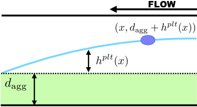
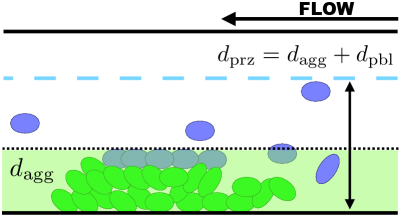
Figure 4: Boundary layers associated with the transport of platelets. Blood flows from right to left, entering the injury channel at $x=0$ and exiting downstream at $x=L_{h}$. (A) Consider a platelet at the position $(x,d_{\text{agg}}+h^{plt}(x))$. The distance it must travel to reach the edge of the growing aggregate is $h^{plt}(x)$ (cyan) and the thickness of the aggregate is denoted as $d_{\text{agg}}$. (B) The PBL thickness at the entrance of the injury channel $h^{plt}(0)$ (cyan, dashed) defines the reaction zone for platelet interactions in that $d_{prz}=d_{\text{agg}}+d_{\text{pbl}}$, where $d_{\text{pbl}}=\min(h^{plt}(0),d_{se})$ and $d_{se}=d_{\text{plt}}=2\ \mu$m.

The advective transport of platelets into and out of each of the platelet compartments is hindered to a degree that depends on the fraction of each compartment’s volume that is occupied by platelets. Let $\theta^{M}=v_{\text{plt}}(P^{m,u}+P^{m,a})$ and $\theta^{B}=v_{\text{plt}}P^{b,a}$, where $v_{\text{plt}}$ is the volume of an individual platelet. The quantities $\theta^{M}$ and $\theta^{B}$ are the volume fractions occupied by mobile and bound platelets, respectively. Note that bound platelets are found only in the aggregate compartments while mobile platelets can be found throughout the injury channel, but we track separately the number densities of mobile platelets in the two PRZs. To describe the transport of mobile, unactivated platelets into the injury channel, we define the quantity

$$J_{\text{prz}}^{in}= \Big{(}\int_{d_{\text{agg}}}^{d_{\text{prz}}}u(y)P^{up}(y)dy\Big{)}W(\theta^{M})\ +\ \Big{(}\int_{0}^{d_{\text{agg}}}u_{\text{}}(y)P^{up}(y)dy\Big{)}W(\theta^{M}+\theta^{B}),$$

where $P^{up}(y)$ is the number density of mobile, unactivated platelets at the inlet to the injury channel. In this work, we assume a uniform and constant upstream distribution $P^{up}(y)=P^{up,*}$, but using non-uniform distributions is straightforward (Appendix D). Note that the use of $P^{up,*}$ in the model yields symmetric top and bottom aggregates. The model framework allows for asymmetric aggregate formation if $P^{up}(y)$ is not symmetric and simulations found in Appendix D explore the resulting aggregates. The function $W$ is intended to limit platelet entry and movement through the region in which the volume fraction of platelets is already high. We used the specific function

$$W(\theta)=\tanh(\pi(1-(\theta/\theta^{\max}))),$$

which monotonically decreases from $W(0)=1$ to $W(1)$ = 0 [24]. Therefore, there is no hinderance when the volume fraction is $0$ and total hinderance as the volume fraction approaches $1$. In choosing this function, we assume that the ability for mobile platelets to move into a region is only gradually impaired until $\theta$ nears $\theta^{\max}=0.6$ and then drops quickly. The rate (number/time), at which mobile, unactivated platelets enter the PRZ is $L_{z}J^{in}_{\text{prz}}$.

We define the following quantities to describe the transport of unactivated and activated mobile platelets out of the injury channel. The rates at which these platelets leave the PRZ are $L_{z}J_{\text{prz}}^{out,u}$ and $L_{z}J_{\text{prz}}^{out,a}$, respectively, where

$$J_{\text{prz}}^{out,u}= \ \Bigg{[}\Big{(}\int_{d_{\text{agg}}}^{d_{\text{prz}}}u(y)dy\Big{)}W(\theta^{M})\ +\ \Big{(}\int_{0}^{d_{\text{agg}}}u(y)dy\Big{)}W(\theta^{M}+\theta^{B})\Bigg{]}P^{m,u},$$

$$J_{\text{prz}}^{out,a}= \ \Bigg{[}\Big{(}\int_{d_{\text{agg}}}^{d_{\text{prz}}}u(y)dy\Big{)}W(\theta^{M})\ +\ \Big{(}\int_{0}^{d_{\text{agg}}}u(y)dy\Big{)}W(\theta^{M}+\theta^{B})\Bigg{]}P^{m,a}.$$

The flow of blood in the injury channel is coupled to the transport of platelets into and out of the injury channel as we describe below.

2.2.2 Cohesion, Adhesion, and Dilution

Platelets contribute to aggregate formation through two binding processes: adhesion and cohesion. Both unactivated and activated mobile platelets can adhere directly to the bottom or top wall of the injury channel. Mobile, activated platelets can cohere to already bound, activated platelets. Platelets are activated through direct contact with the wall or by exposure to the soluble agonist ADP. The activation state of the platelet as well as the available space both on the wall and in the developing aggregate determine which binding processes can occur.

Since adhesion requires that a platelet directly contacts the wall, we limit adhesion to those platelets within a specified distance $d_{se}$ from the walls. In the model, a platelet’s location relative to the walls is only known with respect to whether the platelet is inside one of the PRZs, and so we enforce this limit approximately in the adhesion rate function

$$k_{\text{adh}}(d_{\text{agg}},\theta^{B})=k_{0}^{adh}\min\bigg{(}1-\frac{d_{\text{agg}}}{d_{se}},0\bigg{)}\bigg{(}\theta^{\max}-\theta^{B}\bigg{)},$$

where $k_{0}^{adh}$ is a first order rate constant, the second term represents the accessibility of the wall, and the third term represents the porosity of the aggregate. With this function, adhesion is further limited as the volume fraction of platelets in the aggregate approaches its maximum value $\theta^{\max}$, because platelets already bound to the wall occupy a portion of the wall space available for adhesion. Both unactivated and activated mobile platelets can adhere to the wall and hence the rate of adhesion is proportional to the adhesion rate function and the total number density of mobile platelets.

For mobile platelets to cohere to the aggregate, they must be activated and sufficiently close to activated bound platelets. As previously mentioned, activated platelets have activated integrin receptors on their surfaces that allow for $\alpha_{IIb}\beta_{3}$-fibrinogen-$\alpha_{IIb}\beta_{3}$ and $\alpha_{IIb}\beta_{3}$-vWF-$\alpha_{IIb}\beta_{3}$ bond formation. These bonds are strong, and long-lived with very small off rates. Therefore, we assume that bond breakage is negligible and do not allow for platelet detachment in this model. The rate of platelet-platelet cohesion, $k_{\text{coh}}P^{b,a}P^{m,a}$, depends on the second order rate constant $k_{\text{coh}}$ and the number densities of bound activated platelets, $P^{b,a}$, and mobile, activated platelets $P^{m,a}$, respectively.

In addition to changing the number of bound platelets in the aggregate and the flow through the injury channel, the processes of adhesion and cohesion change the total volume of the aggregate and of the adjacent boundary layers (and therefore of the PRZs) by increasing their thicknesses. For a given number of platelets in the PRZ, an increase in that compartment’s volume results in a decrease in the number density of platelets in it – an effect we refer to as dilution. For example, the term describing this effect on mobile unactivated platelets has the form

$$\Bigg{(}\frac{\frac{d}{dt}(d_{\text{prz}})}{d_{\text{prz}}}\Bigg{)}P^{m,u}_{\text{}},$$

and appears naturally in calculating the rate at which the number of these platelets in the platelet reaction zone changes.

2.2.3 Evolution Equations of Platelets

Here we account for the processes described in Section 2.2.1 and Section 2.2.2 to derive evolution equations for the platelet number densities. Let $V_{\text{prz}}=L_{h}L_{z}d_{\text{prz}}$ denote the volume of the platelet reaction zone. Then the rate of change of the number of mobile, activated platelets in that reaction zone is

$$\underbrace{\frac{d(V_{\text{prz}}P^{m,u})}{dt}}_{\text{rate of change of \# plts}}= \ \underbrace{L_{z}(J_{\text{prz}}^{in}-J_{\text{prz}}^{out,u})}_{\text{flow in/out of reaction zone}}-\underbrace{V_{\text{prz}}k_{\text{act}}P^{m,u}_{\text{}}}_{\text{activation}}-\ \underbrace{V_{\text{prz}}k_{\text{adh}}P^{m,u}_{\text{}}}_{\text{adhesion}}$$

Applying the product rule on the left-hand side and rearranging terms, we determine that

(4) $$\frac{dP^{m,u}}{dt}= \ \underbrace{\frac{(J_{\text{prz}}^{in}-J_{\text{prz}}^{out,u})}{L_{h}d_{\text{prz}}}}_{\text{flow in/out of reaction zone}}-\underbrace{k_{\text{act}}P^{m,u}_{\text{}}}_{\text{activation}}-\ \underbrace{k_{\text{adh}}P^{m,u}_{\text{}}}_{\text{adhesion}}-\underbrace{\Bigg{(}\frac{\frac{d}{dt}(d_{\text{prz}})}{d_{\text{prz}}}\Bigg{)}P^{m,u}_{\text{}}}_{\text{dilution}}.$$

The first and third terms describe transport and adhesion. The second term describes activation of mobile unactivated platelets by exposure to ADP. Based on similar considerations, we find evolution equations for the number densities of the other platelet species $P^{m,a}$ and $P^{b,a}$.

(5) $$\frac{dP^{m,a}_{\text{}}}{dt}= \ \underbrace{-\frac{J_{\text{prz}}^{out,a}}{L_{h}d_{\text{prz}}}}_{\text{flow out of reaction zone}}\ +\ \underbrace{k_{\text{act}}P^{m,u}_{\text{}}}_{\text{activation}}-\underbrace{k_{\text{adh}}P^{m,a}_{\text{}}}_{\text{adhesion}}$$

$$- \ \underbrace{k_{\text{coh}}P^{b,a}_{\text{}}P^{m,a}_{\text{}}}_{\text{cohesion}}\ -\ \underbrace{\Bigg{(}\frac{\frac{d}{dt}(d_{\text{prz}})}{d_{\text{prz}}}\Bigg{)}P^{m,a}}_{\text{dilution}},$$

(6) $$\frac{dP^{b,a}_{\text{}}}{dt}= \ \underbrace{\frac{d_{\text{prz}}}{d_{\text{agg}}}\Big{(}k_{\text{adh}}(P^{m,u}_{\text{}}+P^{m,a}_{\text{}})+k_{\text{coh}}P^{b,a}_{\text{}}P^{m,a}_{\text{}}\Big{)}}_{\text{adhesion and cohesion}}-\ \underbrace{\Bigg{(}\frac{\frac{d}{dt}(d_{\text{agg}})}{d_{\text{agg}}}\Bigg{)}P^{b,a}_{\text{}}}_{\text{dilution}}.$$

2.3 Soluble Agonist ADP

An unactivated platelet stores quantities of ADP in its dense granules and releases this ADP into the surrounding fluid when the platelet is activated. Similar to the treatment in [24], we assume this release occurs during the time interval 1-5s after activation. Once released, that ADP moves by advection and diffusion within and out of the aggregate where it can activate mobile platelets. Describing these processes requires defining two boundary layers: one within the aggregate $h^{adp}_{\text{agg}}(x)$ and one in the Stokes region $h^{adp}_{\text{BL}}(x)$. These boundary layers are used to define the ADP compartments shown in Fig. 2C and the ADP concentrations tracked are those inside the aggregate $[ADP]_{\text{agg}}$, in the Stokes region boundary layer $[ADP]_{\text{BL}}$, and in the remaining Stokes region which we denote as $[ADP]_{\text{gap}}$.

(A)                                                      (B)

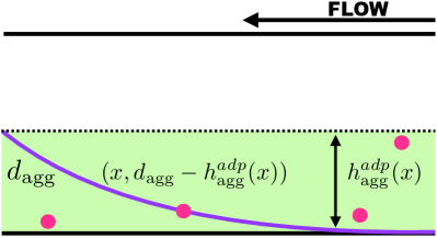
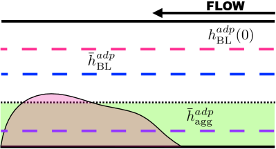
Figure 5: Boundary layers associated with the transport of soluble agonist ADP. (A) Consider an ADP molecule at the position $(x,d_{\text{agg}}-h^{adp}_{\text{agg}}(x))$. The distance it must travel to reach the edge of the growing aggregate is $h^{adp}_{\text{agg}}(x)$. (B) The boundary layer thickness at the entrance of the injury channel in the Stokes region is $h^{adp}_{BL}(0)$ (magenta, dashed) and defines the reaction zone for ADP interactions in that region (ARZ). Both the average thickness in the Stokes region $\bar{h}^{adp}_{BL}$ (blue, dashed) and in the growing aggregate $\bar{h}^{adp}_{\text{agg}}$ (purple, dashed) are used to define diffusive transport from the aggregate into the Stokes region.

2.3.1 Boundary Layer Calculations

The first boundary layer is related to ADP movement in the Stokes region after it has left the aggregate where it is released. The calculation is like that for platelets in the Stokes region as described above in Section 2.2.1. This boundary layer is thinnest at the upstream end and widest at the downstream end. Its thickness is greater than that, $h^{plt}(x)$, of the platelet boundary layer. This is because (i) ADP has a larger diffusivity than platelets and (ii) the choice of velocity used in the boundary layer calculation. For the platelets, it is a velocity in the Stokes region $u(d_{\text{agg}}+h^{plt}(x))$ and for the ADP it is the (lower) velocity on the edge of the Stokes region $u(d_{\text{agg}})$. Therefore, $h^{adp}_{\text{BL}}(x)>h^{plt}(x),\forall x\in[0,L_{h}]$. As shown in Fig. 5B, the maximum thickness of this ADP boundary layer in the Stokes region is denoted as $h^{adp}_{\text{BL}}(0)$ and the average boundary layer thickness as $\bar{h}^{adp}_{\text{BL}}$.

The second boundary layer describes ADP movement within the aggregate towards the Stokes region and requires the new calculation given in this section. We do not have a separate ADP concentration in this boundary layer; its thickness is used only in calculating the ADP concentration gradient. Consider the starting point $(x,d_{\text{agg}}-h_{\text{agg}}^{adp}(x))$ inside the aggregate and equate the time it takes an ADP molecule there to diffuse into the Stokes region with the time it would take it to be washed past the injured region by the flow:

$$\frac{(d_{\text{agg}}-h_{\text{agg}}^{adp}(x))^{2}}{2D_{a}}=\frac{L_{h}-x}{u(d_{\text{agg}})}.$$

We solve for the thickness $h^{adp}_{\text{agg}}(x)$ and define $\bar{h}^{adp}_{\text{agg}}$ to be the average aggregate layer thickness shown in Fig. 5B. The ADP boundary layer thickness $d_{\text{abl}}=h^{adp}_{\text{BL}}(0)$ and the thickness of the growing aggregate contribute to the total thickness of the regions in which we track the ADP concentrations: $[ADP]_{\text{agg}}$, $[ADP]_{\text{BL}}$, and $[ADP]_{\text{gap}}$.

2.3.2 ADP Release and Advection

The source of ADP in this model corresponds to the release of ADP from activated, bound platelets. The rate of release is

$$\sigma_{\text{release}}(t)=\int_{0}^{\infty}\hat{A}R(\tau)\frac{d}{dt}(P^{b,a})(t-\tau)d\tau,$$

where $\hat{A}$ (Appendix C) is the total quantity of ADP released by an activated platelet, $\hat{A}R(\tau)$ is the rate of release at an elapsed time since activation $\tau$ and $\int_{0}^{\infty}R(\tau)d\tau=1$. The function $R(\tau)$ is defined as having value zero up to one second after activation, a positive bell-shaped function for the time interval $1<\tau<5$ seconds, and a peak at three seconds. The term $\frac{d}{dt}(P^{b,a})(t-\tau)d\tau$ is the number of platelets newly activated and bound in the time interval $[t-\tau,t-\tau+d\tau]$. We account only for ADP release from bound activated platelets because activated platelet that do not become bound are carried downstream before they begin to release their ADP.

To facilitate our describing the advective transport of ADP out of the aggregate, the boundary layer, and the gap, we define the expressions

$$J_{\text{agg}}^{adp} =\Big{(}\int_{0}^{d_{\text{agg}}}u_{\text{}}(y)dy\Big{)}[ADP]_{\text{agg}},$$

$$J_{\text{BL}}^{adp} =\Big{(}\int_{d_{\text{agg}}}^{d_{\text{agg}}+d_{\text{abl}}}u(y)dy\Big{)}[ADP]_{\text{BL}},$$

$$J_{\text{gap}}^{adp} =\Big{(}\int_{d_{\text{agg}}+d_{\text{abl}}}^{d_{\text{agg}}+d_{\text{abl}}+d_{\text{gap}}}u(y)dy\Big{)}[ADP]_{\text{gap}},$$

respectively. Then, the rates of advective transport of ADP out of the ADP compartments in the injury channel are $L_{z}J^{adp}_{\text{agg}}$, $L_{z}J^{adp}_{\text{BL}}$, and $L_{z}J^{adp}_{\text{gap}}$. Early on, the magnitude of the velocity and the thicknesses of the aggregate and boundary layers lead to the ordering $J_{\text{gap}}^{adp}>J_{\text{BL}}^{adp}>J_{\text{agg}}^{adp}$. As the aggregate grows, the boundary layers become larger, decreasing the thickness of the gap $d_{\text{gap}}$ and resulting in a new ordering $J_{\text{BL}}^{adp}>J_{\text{gap}}^{adp}$. If the flow is slowed sufficiently, $d_{\text{gap}}=0$ and $J_{\text{gap}}^{adp}=0$.

(A)                                                        (B)

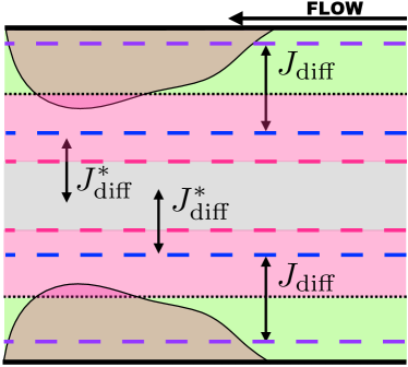
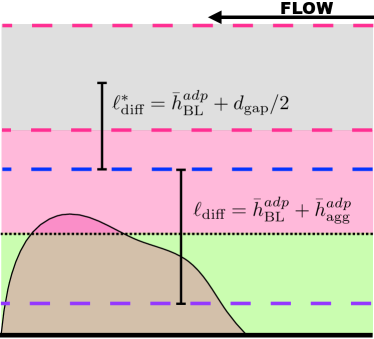
Figure 6: Compartment model describing diffusive transport of ADP. (A) Diffusive fluxes of ADP from the aggregates (green) to the associated boundary layers (blue) are denoted as $J_{\text{diff}}$. ADP also diffuses from the boundary layers associated with the bottom and top aggregates to the bulk of the Stokes region (pink) with flux $J_{\text{diff}}^{*}$. The fluxes are subject to changing layer thickness that are determined by the flow velocity. (B) The dashed lines correspond to boundary layers associated with the bottom aggregate. The specified lengths $\ell_{\text{diff}}$ and $\ell_{\text{diff}}^{*}$ are used to define the gradients of ADP concentration between the aggregates and boundary layers as well as between boundary layers and bulk Stokes region, respectively.

2.3.3 Diffusive Transport of ADP

Diffusive transport of ADP from the aggregate into the boundary layer and into the bulk Stokes region also changes the ADP concentrations. The diffusive transport of ADP (Fig. 6A) between the aggregate (green) and the boundary layer region (pink) and that between boundary layer and the bulk Stokes region (grey) are determined using Fick’s law [11]. Let $V_{\text{abl}}=L_{h}L_{z}d_{\text{abl}}$ be the volume of the ADP boundary layer and $\ell_{\text{diff}}$ be the length that determines the gradient of ADP from the aggregate to the boundary layer. As shown in Fig. 6B, this length is the distance between the edge of the boundary layer in the aggregate (purple, dashed) and the edge of the average boundary layer in the Stokes region (dashed, blue). The diffusive flux of ADP from the aggregate into the boundary layer is

$$J_{\text{diff}} =D_{a}\frac{([ADP]_{\text{agg}}-[ADP]_{\text{BL}})}{c_{1}\ell_{\text{diff}}},$$

and the rate of diffusion is $L_{h}L_{z}J_{\text{diff}}$, where $L_{z}L_{h}$ is the area of the interface between the zones, $D_{a}$ is the diffusion coefficient, $([ADP]_{\text{agg}}-[ADP]_{\text{BL}})$ is the difference in ADP concentration between the aggregate and the boundary layer, and $\ell_{\text{diff}}$ is the length used to define the gradient. Similarly, the diffusive flux of ADP from the boundary layer into the ‘gap’ is

$$J_{\text{diff}}^{*} =D_{a}\frac{([ADP]_{\text{BL}}-[ADP]_{\text{gap}})}{c_{2}\ell_{\text{diff}}^{*}},$$

where the rate of transport flux is $L_{h}L_{z}J_{\text{diff}}^{*}$, $([ADP]_{\text{BL}}-[ADP]_{\text{gap}})$ is the difference in ADP concentration and $\ell_{\text{diff}}^{*}$ is half the distance between the edge of the boundary layer and the center of the gap. The fitted parameters $c_{1}$ and $c_{2}$ are discussed in Appendix C.

2.3.4 Evolution Equations for ADP

Accounting for release, transport due to advection, and diffusive transport between the aggregates, boundary layer regions, and the gap in the Stokes region, the ADP concentrations in the aggregate and boundary layer region evolve according to the equations

(7) $$\frac{d[ADP]_{\text{agg}}}{dt}= \ \underbrace{\sigma_{\text{rel}}(t)}_{\text{release}}\ -\ \underbrace{\frac{J_{\text{diff}}}{d_{\text{agg}}}}_{\parbox{21.00005pt}{\scriptsize diffusion into BL}}\ -\ \underbrace{\frac{J_{\text{agg}}^{adp}}{L_{h}d_{\text{agg}}}}_{\text{flow out of agg}}-\underbrace{\bigg{(}\frac{\frac{d(d_{\text{agg}})}{dt}}{d_{\text{agg}}}\bigg{)}[ADP]_{\text{agg}}}_{\text{dilution}},$$

and

(8) $$\frac{d[ADP]_{\text{BL}}}{dt}= \underbrace{\frac{J_{\text{diff}}}{d_{\text{abl}}}}_{\parbox{21.00005pt}{\scriptsize diffusion into BL}}-\underbrace{\frac{J^{*}_{\text{diff}}}{d_{\text{abl}}}}_{\parbox{21.00005pt}{\scriptsize diffusion into gap}}\ -\ \underbrace{\frac{J_{\text{BL}}^{adp}}{L_{h}d_{\text{abl}}}}_{\text{flow out of BL}}-\underbrace{\bigg{(}\frac{\frac{d(d_{\text{abl}})}{dt}}{d_{\text{abl}}}\bigg{)}[ADP]_{\text{BL}}}_{\text{dilution}},$$

The concentration of ADP in the gap changes because of diffusive transport from both the bottom and top boundary layers:

(9) $$\frac{d[ADP]_{\text{gap}}}{dt}= \underbrace{\ \ \ \frac{J^{*}_{\text{diff,b}}}{d_{\text{gap}}}\ \ \ }_{\text{\parbox{42.00009pt}{\scriptsize diffusion into gap from bottom}}}\ +\ \underbrace{\ \ \ \frac{J^{*}_{\text{diff,t}}}{d_{\text{gap}}}\ \ \ }_{\parbox{42.00009pt}{\scriptsize diffusion into gap from top}}\ -\ \underbrace{\frac{J_{\text{gap}}^{adp}}{L_{h}d_{\text{gap}}}}_{\text{flow out of gap}}-\underbrace{\bigg{(}\frac{\frac{d(d_{\text{gap}})}{dt}}{d_{\text{gap}}}\bigg{)}[ADP]_{\text{gap}}}_{\text{dilution}},$$

where $J^{*}_{\text{diff,b}}$ and $J^{*}_{\text{diff,t}}$ are the respective diffusive fluxes of ADP into the gap from the bottom and top boundary layers.

2.4 Aggregate Formation

The formation of the aggregate layer is described by its evolving thickness, $d_{\text{agg}}$, and volume fraction of bound platelets, $\theta^{B}$. To determine evolution equations for these quantities, one must consider the adhesion and cohesion events that contribute to the change in volume occupied by bound platelets. Let $V_{\text{agg}}=L_{h}L_{z}d_{\text{agg}}$. The rate of change of the volume occupied by bound platelets is

$$\frac{d}{dt}(V_{\text{agg}}\theta^{B})=\underbrace{V_{\text{prz}}k_{\text{adh}}(P^{m,u}+P^{m,a})v_{\text{plt}}}_{\text{adhesion of mobile plts.}}\ +\ \underbrace{V_{\text{prz}}(k_{\text{coh}}P^{b,a}P^{m,a})v_{\text{plt}}}_{\text{cohesion of mobile, act. plts}}.$$

Dividing by $d_{\text{agg}}\theta^{B}$ and using the product rule, and partitioning the adhesive term and cohesion term we find the following equations.

(10) $$\frac{d\theta^{B}_{\text{}}}{dt}= \ \gamma_{\text{}}\bigg{(}\frac{d_{\text{prz}}}{d_{\text{agg}}}\bigg{)}k_{\text{adh}}\Big{(}P^{m,u}_{\text{}}+P^{m,a}_{\text{}}\Big{)}v_{\text{plt}}\ +\ \beta_{\text{}}\bigg{(}\frac{d_{\text{prz}}}{d_{\text{agg}}}\bigg{)}k_{\text{coh}}\Big{(}P^{b,a}_{\text{}}P^{m,a}\Big{)}v_{\text{plt}}$$

(11) $$\frac{d}{dt}(d_{\text{agg}})= \ (1-\gamma_{\text{}})(d_{\text{prz}})k_{\text{adh}}\bigg{(}\frac{P^{m,u}_{\text{}}+P^{m,a}_{\text{}}}{P^{b,a}_{\text{}}}\bigg{)}\ +\ (1-\beta_{\text{}})(d_{\text{prz}})k_{\text{coh}}\bigg{(}\frac{P^{b,a}_{\text{}}P^{m,a}_{\text{}}}{P_{\text{}}^{b,a}}\bigg{)},$$

where $\beta_{\text{}}$, $\gamma_{\text{}}$ are assumed to have the functional forms

$$\gamma=\begin{cases}0,\text{ if }\theta^{B}=\theta^{\max}\\ 1,\text{ if }d_{\text{agg}}\geq d_{\text{plt}}\end{cases}\beta=\begin{cases}\frac{1}{2}(1+\tanh(k_{b}(s_{b}-\theta^{B}))),\text{ if }d_{\text{gap}}>0,\theta^{B}<\theta^{\max}\\ 0,\text{ if }\theta^{B}=\theta^{\max}\\ 1,\text{ if }d_{\text{gap}}=0\end{cases}.$$

The partition functions $\beta$ and $\gamma$ are phenomenological in nature and will be partially validated by PDE model (Section A.4). Details are found in Appendix C. Equations (4)-(11) describe platelet dynamics, ADP dynamics, and aggregate formation associated with the bottom wall of the injury zone. There is a similar set of equations governing the concentrations of platelets species, ADP, aggregate thickness, and aggregate volume fraction associated with the top aggregate.

2.5 Platelet Activation

As noted above, once an unactivated platelet enters the PRZ it can adhere to the wall and therefore become bound and activated, it can be activated by ADP and possibly cohere to already bound platelets, or it can be carried out of the injury channel by the flow. While platelet activation is a complex process triggered by a range of stimuli and made up of an ensemble of responses [27], we focus on activation by direct adhesion to the wall and by exposure to ADP and on the resulting activation of integrin $\alpha_{IIb}\beta_{3}$ receptors and release of ADP. We discussed the activation by direct adhesion above. Activation triggered when ADP in the plasma binds to a platelet’s P2Y₁ and P2Y₁₂ receptors, provides a means of activation that does not require contact with the SE matrix. Because ADP stimulates this activation and additional ADP is released as a consequence, there is a positive feedback in the system involving the concentration of ADP and the transition of mobile, unactivated platelets to mobile, activated platelets. To model ADP-dependent activation, we assume that the activation trigger is a weighted average of the ADP concentrations in the aggregate and in the boundary layer. We define the rate of ADP-induced activation as

$$k_{\text{act}}=k^{act}_{0}A([ADP]_{\text{agg}},[ADP]_{\text{BL}}),$$

where

$$A([\text{ADP}]_{\text{agg}},[\text{ADP}]_{\text{BL}})=\bigg{(}\frac{d_{\text{agg}}}{d_{\text{arz}}}\bigg{)}\frac{[\text{ADP}]_{\text{agg}}}{[\text{ADP}]^{*}+[\text{ADP}]_{\text{agg}}}+\bigg{(}\frac{d_{\text{pbl}}}{d_{\text{arz}}}\bigg{)}\frac{[\text{ADP}]_{\text{BL}}}{[\text{ADP}]^{*}+[\text{ADP}]_{\text{BL}}}.$$

Here, $d_{\text{arz}}=d_{\text{agg}}+d_{\text{abl}}$ is the thickness of the ADP reaction zone (ARZ) and $[ADP]^{*}=1\mu$M. For some of our simulations, we instead considered ADP-independent platelet activation in the plasma by setting $A([\text{ADP}]_{\text{agg}},[\text{ADP}]_{\text{BL}})\equiv 1$, in which case only the value of the rate constant $k^{act}_{0}$ matters. Below we explore the effects of ADP-independent versus ADP-dependent activation on aggregate growth and occlusion of the injury channel.

2.6 Numerical Methods

Simulations of the ODE model consist of solving the HC system and the Brinkman-Stokes system to determine $G_{h}$ and $R_{M}$, respectively. The differential equations describing the evolution of platelet species, ADP, and aggregate thickness and density are solved using MATLAB function ode15s, which employs a variable-step, variable-order (VSVO) solver based on the numerical differentiation formulas (NDFs) of orders 1 to 5 for stiff systems [41]. During each time step of the computation, we perform the following series of updates for the unknowns.

1. Assume $G_{h}=1$ and solve the linear system in Appendix B to determine $u(y)$ and $R_{M}$.

2. Use $R_{M}$ as an input parameter for the HC system in Appendix A and solve for $G_{h}$.

3. Scale the flow velocity using the pressure gradient update; $\bar{u}(y):=G_{h}u(y)$.

4. Use $u(y)$ and diffusivity constants ($D_{p}$, $D_{a}$) to determine boundary layers ($h^{plt}(x)$, $h^{adp}_{\text{BL}}(x)$, $h^{adp}_{\text{agg}}(x)$) for both aggregates.

5. Determine thicknesses of the PRZ ($d_{\text{prz}}$), compartments in the Stokes region tracking ADP ($d_{\text{abl}}$, $d_{\text{gap}}$), and the growing aggregate ($d_{\text{agg}}$) associated with the bottom and top walls.

6. Count the platelets activated within the previous time step and update the ADP release function $\sigma_{rel}$ for each aggregate.

7. Update mobile platelets and ADP concentrations associated with the top and bottom aggregates and reaction zones to account for advection using the velocity profile $u(y)$.

8. Update ADP concentrations to account for diffusion using ADP boundary layer thicknesses ($\bar{h}^{adp}_{\text{BL}}$, $\bar{h}^{adp}_{\text{agg}}$) of the top and bottom ARZs and aggregates.

9. Update the thicknesses of the aggregates $d_{\text{agg}}$, the volume fractions of bound platelets $\theta^{B}$, and hinderance function $W(\theta^{B}+\theta^{M})$ to account for platelet adhesion and cohesion events.

10. Repeated until desired time.

The simulations described below were carried out for 20 minutes and all parameters values are found in Table 1-Table 7 with specific details in Appendix A - Appendix C. Each simulation requires $\approx 50$ seconds of computational time. This computational cost can be substantially reduced by using a compiled language.

3 Results

The presented mathematical model was calibrated and validated through comparisons of model output with that of analogous MFA (Section A.2) and PDE (Section A.4) models. Preliminary studies with the PDE model revealed that the pressure drop $\Delta P=P_{1}-P_{2}$ across the injury channel was not constant with respect to the y-direction. Therefore to achieve the most accurate model comparisons, it was necessary to compute an approximation of the flow rate $Q_{PDE}$ through the injury channel using the PDE model for all the following simulations. This changes the second step of our numerical scheme. Specifically, we do not solve the HC system for the pressure gradient $G_{h}$. Instead, we assume

$$G_{h}=\frac{Q_{PDE}(d_{b},d_{t},\theta^{B}_{b},\theta^{B}_{t})}{R_{M}L_{h}^{\text{eff}}},$$

where $d_{b},d_{t}$ and $\theta^{B}_{b},\theta^{B}_{t}$ are the thicknesses and densities of the bottom and top aggregates, respectively. The effective length of the channel, $L_{h}^{\text{eff}}=165\ \mu\text{m}$ as described in Section A.1. Details regarding $Q_{PDE}$ are found in Figure 7A-B and Section A.3. Note that the ODE model is not dependent on the use of the PDE flow map and the use of the ODE model beyond the scope of this work is independent of PDE model results.

Using this new calculation for the pressure gradient, we validated the fluid calculation associated with the ODE model in Fig. 7C-D. Assuming ADP-independent platelet activation ($A([ADP]_{\text{agg}},[ADP]_{\text{BL}})=1$), we used MFA occlusion times to determine physiologically relevant values for the kinetic rate constant $k^{adp}_{0}$ (Fig. 8A-B). Fixing a value for $k^{adp}_{0}$, we compared occlusion metrics Fig. 8C-D from the ODE and PDE models. Next, we assessed and characterized occlusion of the injury channel as a function of the flow shear rate and $k^{adp}_{0}$ in Fig. 9A-B and then conducted similar experiments to test the sensitivity of model output to ADP-dependent platelet activation as shown in Fig. 10A-D. Evidence of the effects of dilution of ADP due to advective and diffusive transport on aggregate formation is found in Fig. 11A-H.

3.1 Model Validation and Calibration

(A)                                                 (B)

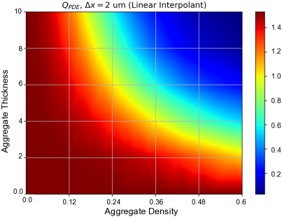
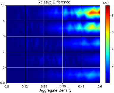
(C)                                                 (D)

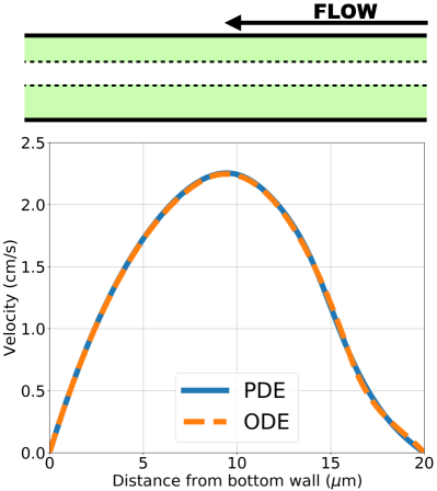
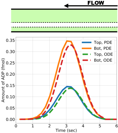
Figure 7: Model calibration and validation. (A) 3D flow rates $Q_{PDE}$ in prebound platelet simulations with the PDE model using spatial discretization $\Delta x=2\ \mu$m and (B) the relative difference between the flow rates generated with ($\Delta x=2\ \mu$m) and ($\Delta x=1\ \mu$m). (C) Velocity profiles from ODE and PDE models for an asymmetric prebound platelet configuration ($d_{t}=6\mu$m, $\theta^{B}_{t}=0.54$, $d_{b}=8\mu$m, $\theta^{B}_{b}=0.06$). (D) Similar prebound platelet configuration ($d_{t}=12\mu$m, $\theta^{B}_{t}=0.15$, $d_{b}=4\mu$m, $\theta^{B}_{b}=0.45$) experiment tracks the amount of ADP in the aggregate for the PDE and ODE models. Note $\theta^{\max}=0.6$.

For this study, we simulated 2D flow through the injury channel with fixed pre-formed platelet aggregates. For each simulation, a different symmetric configuration of preformed aggregates was specified by choosing the thicknesses $d_{\text{b}}=d_{\text{t}}\in\{2,4,6,8,10\ \mu m\}$ and bound platelet densities $\theta^{B}_{\text{b}}=\theta^{B}_{\text{t}}\in[0.0,0.06,\cdots 0.6]$. The PDE model was used to calculate the steady-state velocity field and two-dimensional volumetric flow rate $Q_{PDE}$ for each configuration as detailed in Section A.3. The ‘flow map’ $Q_{PDE}(d_{\text{b}},\theta^{B}_{\text{b}},d_{\text{t}},\theta^{B}_{\text{t}})$ obtained when the PDE calculation used a spatial discretization with step size $\Delta x=2\ \mu$m is shown in Fig. 7A, and Fig. 7B presents evidence that the flow rate calculation is insensitive to further refinement in $\Delta x$. The maximum relative difference in flow rates for the two stepsizes, which occured for an aggregate density of $\approx 0.5$ and with almost-occlusive thicknesses of $\approx 9.5\ \mu m$, was approximately $8(10)^{-7}$.

(A)                                                 (B)

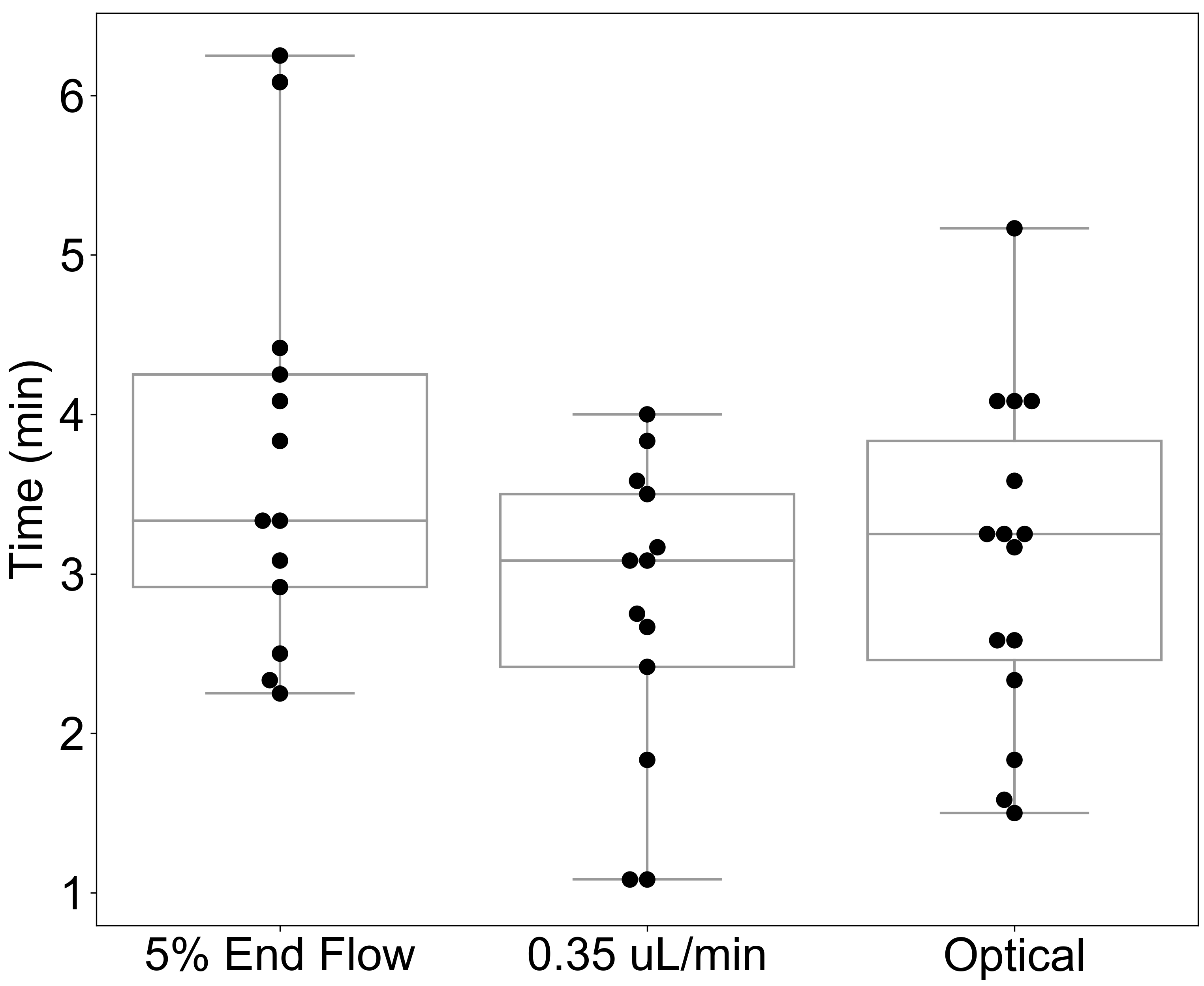
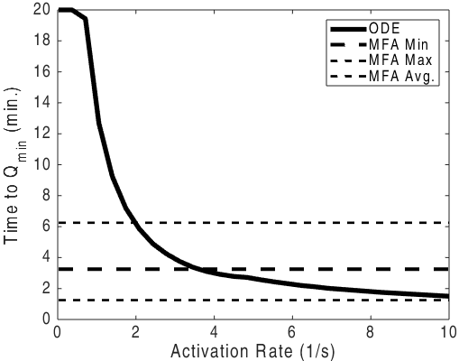
(C)                                                 (D)

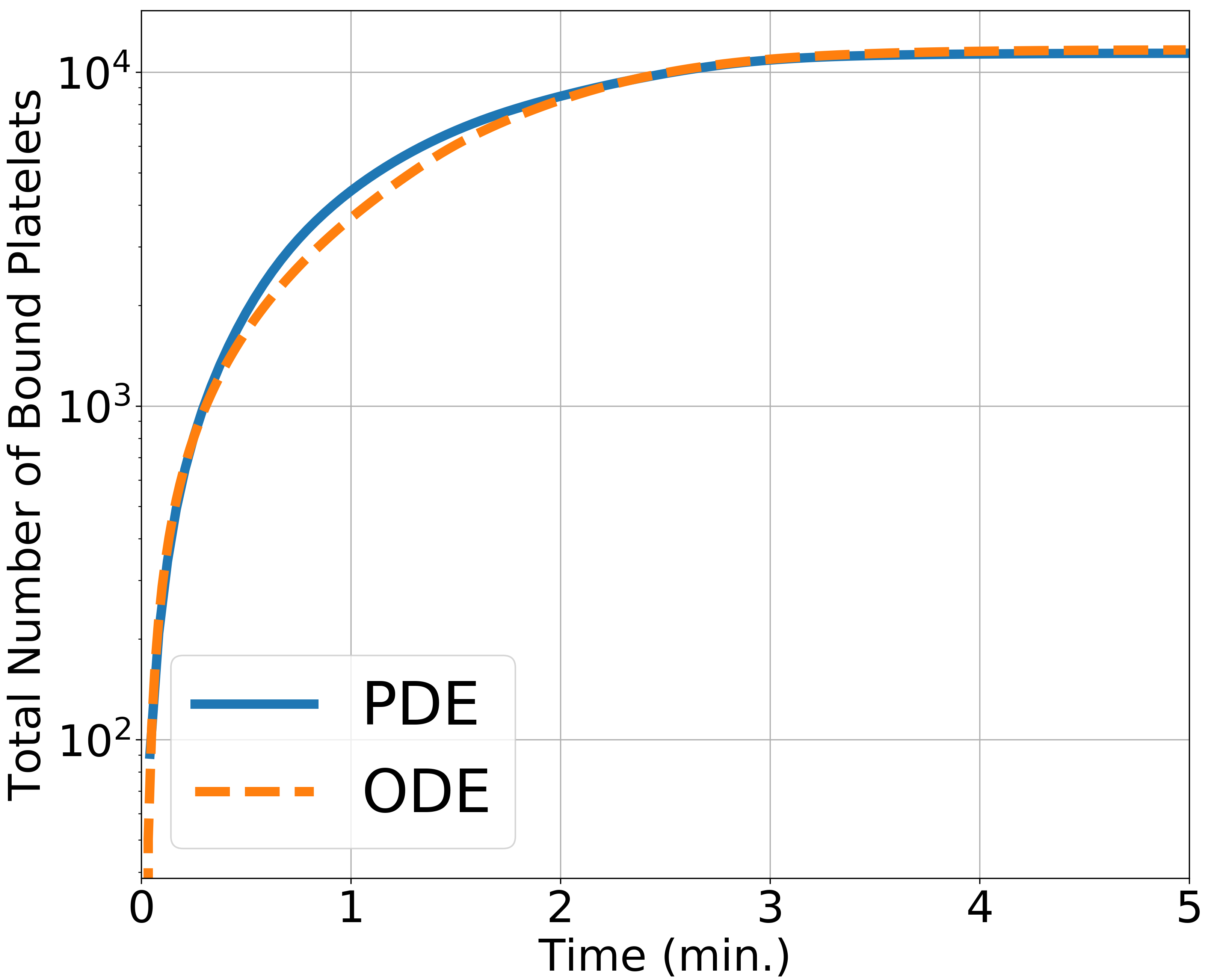
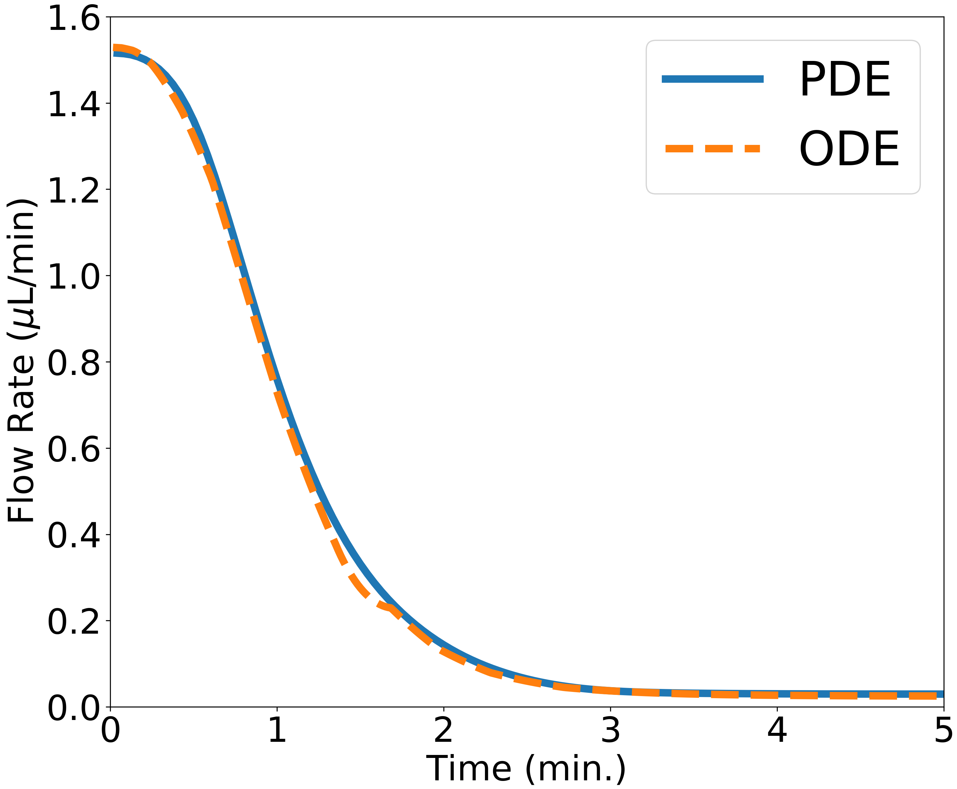
Figure 8: Model calibration and validation.(A) Occlusion times generated by the MFA bleeding chip and (B) ODE model times to $Q_{\min}=0.35\ \mu$L/min as a function of the ADP-independent platelet activation rate $k^{act}_{0}$. Comparison of ODE (orange) and PDE (blue) model outputs with a fixed shear rate ($\approx 2400\ \text{s}^{-1}$) and ADP-independent platelet activation rate ($k^{act}_{0}=3.4\text{ s}^{-1}$). (C) Total number of bound platelets in the aggregate and (D) rate of blood flow through the injury channel.

Fig. 7C shows velocity profiles from the ODE and PDE models for asymmetric aggregates. The ODE profile shows excellent agreement in both Brinkman layers and the Stokes region with the PDE profile obtained half-way through the injury channel. The flow through the top aggregate, which is thin ($d_{\text{t}}=4\ \mu$m) but dense ($\theta^{B}_{\text{t}}=0.54$) is slower than that in the thick ($d_{\text{b}}=8\ \mu$m) yet loose ($\theta^{B}_{\text{b}}=0.06$) bottom aggregate, because resistance to flow increases as aggregate density increases.

In Fig. 7D, we show results from another asymmetric pre-formed aggregate configuration, assuming that all of the platelets in the aggregates became activated at time $t=0$. Shown are the amounts of ADP in each of the aggregates due to release of ADP by these platelets in both the ODE and PDE models. Less ADP is washed downstream from the thin and dense bottom aggregate because the flow in it is slower. Consequently, the maximum concentration of ADP in the bottom aggregate is higher than that in the thick and loose top aggregate (not shown). It is important to note that the concentration of ADP in each aggregate is subject to diffusive transport. The ODE model accounts for lateral diffusion (perpendicular to the channel walls) but not longitudinal diffusion. The differences in the models’ outputs are largely due to longitudinal diffusion of ADP out of the injury channel in the PDE model (results not shown).

One of our main objectives in this work was to develop a mathematical model that can generate aggregates that grow to fill the injury channel. This objective was motivated by experiments conducted in the microfluidic bleeding chip model (MFA). Fig. 8A shows three metrics of occlusion times from experiments using the MFA. The median times for all three metrics of occlusion are approximately 3.25 minutes, with a minimum occlusion time of 1.15 minutes and a maximum time of 6.25 minutes. The metric of occlusion best suited for comparison with the ODE model output is the ‘time to $Q_{\min}=0.35\ \mu$L/min measurement’. Using an ADP-independent platelet activation regime $(A([\text{ADP}]_{\text{agg}},[\text{ADP}]_{\text{BL}})\equiv 1)$ in the ODE model simulations yields the ‘time to Q${}_{\text{min}}$’ results obtained for a range of platelet activation rates as shown in Fig. 8B. For $k^{act}_{0}>2.0\ \text{s}^{-1}$, the time to $Q_{\min}$ is within the bounds defined by the MFA results. In Fig. 8C-D, we compare the growth of aggregates using the ODE model (orange) with output from the PDE model (blue). Metrics are the timecourse of the total number of bound platelets and of the flow rate through the injury channel. For a fixed shear rate $\approx 2400\text{ s}^{-1}$ and a fixed platelet activation rate of $3.4\ \text{s}^{-1}$, model results fall within the range of the experimental values. Note that in Fig. 8B, the time to $Q_{\min}$ with the chosen activation rate is within the range (black, dashed lines) seen with the MFA. Additionally, both computational models yielded aggregates that reduced the flow rate of the injury channel in an amount of time similar to that seen in the MFA results.

3.2 Occlusion of Injury Channel and Flow Rate Reduction

To better understand how shear rate and ADP-independent platelet activation affect aggregate formation, we performed simulations in which we varied both the shear rate and activation rate constant $k^{act}_{0}$.

(A)                                                        (B)

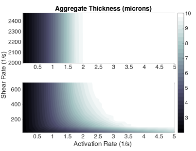
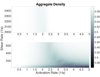
Figure 9: Occlusion in the Injury Channel with ADP-independent activation. ODE model aggregate (A) thicknesses ($\mu$m) and (B) densities due to variations in ADP-independent platelet activation rates $k^{adp}_{act}$ and shear rate $\gamma$, after 10 minutes of simulation time.

Aggregate thickness $d_{\text{agg}}$ and aggregate density $\theta^{B}$ after 10 minutes of simulation time are shown in Fig. 9A-B. For shear rates $200\text{ s}^{-1}<\gamma<2400\text{ s}^{-1}$, occlusive aggregates formed if $k^{act}_{0}>2.0\text{ s}^{-1}$ while significantly thinner but high density aggregates form for $k^{act}_{0}$ below approximately 1.5 s^-1. For shear rates less than $100\text{ s}^{-1}$, aggregate thickness increases as $k^{act}_{0}$ is increased, but in contrast to what is seen for high shear rates, the aggregate density decreased as the activation rate constant was increased from $1.0$ to $5.0\text{ s}^{-1}$. Hence the model predicts that occlusive aggregates form under a wide range of shear rates provided platelet activation rate is large enough, but the nature of the aggregates is sensitive to activation rate especially at low shear rates.

3.3 Dilution of Chemical Agonists

In this section we turn to the model’s behavior when the platelet activation rate is dependent on the ADP concentration $k^{plt}_{act}=k^{act}_{0}$ $A([\text{ADP}]_{\text{agg}},[\text{ADP}]_{\text{BL}})$. If the ADP concentration is substantially below the transition concentration $[\text{ADP}]^{*}=1\mu$M in this function, results might be very different from those just reported with a constant rate of platelet activation.

(A)                                                        (B)

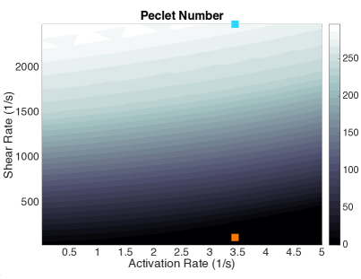
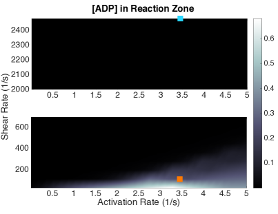
(C)                                                        (D)

Figure 10: Aggregate Heterogeneity under variations in flow conditions and ADP-dependent platelet activation. (A) Peclet number describing the advective versus diffusive transport of soluble agonist ADP. (B) Concentration of ADP in the aggregate and associated boundary layer. (C) Aggregate thickness and (D) aggregate density as functions of shear rate and platelet activation rate constant. These results identified two flow regimes for a fixed platelet activation rate constant $k^{act}_{0}=3.4\ \text{s}^{-1}$; high shear (cyan square) and low shear (orange square). The metrics are taken after 10 minutes of simulation time.

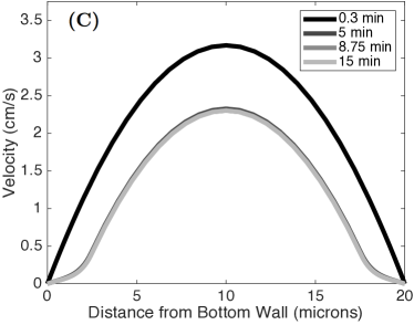
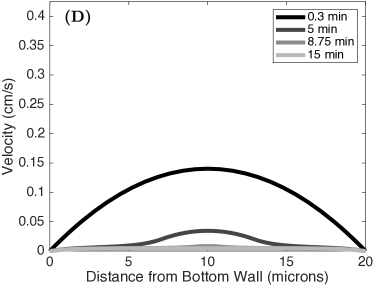
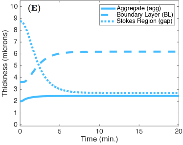
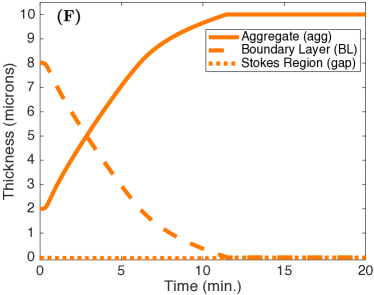
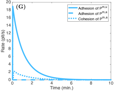
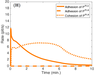
Figure 11: Effect of ADP Dilution on Aggregate Formation. ADP concentrations in the aggregate, boundary layer, and gap under (A) high and (B) low shear conditions. Note there is no gap in the low shear conditions due to the thicknesses of the aggregate and boundary layer. The grey-scale squares denote the times at which the velocity profiles were determined. Velocity profiles at 0.3, 5, 8.75, and 15 minutes under (C) high and (D) low shear conditions. Thicknesses of the aggregate, boundary layer, and gap under (E) high and (F) low shear conditions. The rates of adhesion and cohesion under high (G) and low (H) shear conditions.

We explored how different forms of transport within the aggregates affects their growth by calculating the ADP-related Peclet number after 10 minutes of simulation time. This non-dimensional number is defined as the ratio of the rate of advection by flow and the rate of diffusion of ADP. For our purposes

$$\text{Pe}=\frac{d_{\text{abl}}\ u(d_{\text{apz}})}{D_{a}},$$

where $u(d_{\text{apz}})$ is the velocity at the edge of the ADP boundary layer in the Stokes region ($d_{\text{apz}}=d_{\text{agg}}+d_{\text{abl}}$). Fig. 10A shows that advective transport dominates for shear rates greater than $500\text{ s}^{-1}$ for activation rate constants $k_{0}^{act}$ ranging from $0.02-5.0\text{ s}^{-1}$, but that, while still large, it is much lower for shear rates less than $200\text{ s}^{-1}$. We can see that for most of the shear rate range, the concentration of ADP in the PRZ after 10 minutes is much less that the activation transition concentration $[\text{ADP}]^{*}=1\ \mu$M and that the shear rate must be reduced to below $\approx 100\text{ s}^{-1}$ for the ADP concentration to reach $0.4\ \mu$M. As shown in Fig. 10B, increasing the value of $k_{0}^{act}$ results in higher ADP concentrations. Plots of aggregate thicknesses and densities in Fig. 10C-D identify two flow regimes that for a fixed activation rate constant yield occlusive aggregates under low shear conditions and thin non-occlusive, but dense, aggregates under high shear conditions.

To better understand the differences in aggregates that form under high shear (cyan squares in Fig. 10) and low shear (orange squares in Fig. 10) conditions, we consider the model output in Fig. 11A-H. The initial rate of adhesion is greater in high shear case (Fig. 11G,H) because of the faster replenishment of platelets by the faster flow. Hence, the initial rate of ADP release is also greater in this case. Despite this, the ADP concentrations are more than 6-fold lower (Fig. 11A,B) because the faster flow carries ADP away more rapidly. In the low shear case, the two ADP boundary layers (ABL) are so thick (Fig. 11E,F) that there is no gap region in that case. For both shear conditions, the velocity through the injury channel decreases as the aggregates form. The reduction in peak velocity is approximately 30% after 15 minutes in the high shear case (Fig. 11C), while the relative reduction is much greater, at approximately 80%, under low shear (Fig. 11D). This larger reduction in velocity results in lower rate of advective transport and consequentially increases the boundary layer thickness (orange, dashed) for ADP (Fig. 11F). As the aggregate grows, this layer becomes smaller until the injury channel occludes. Because platelet activation by ADP continues in the low shear case, ADP continues to be released and its concentration remains significant for the entire period leading up to occlusion.

4 Discussion

We developed the first mathematical model of flow-mediated primary hemostasis in an extravascular injury which is able to track the process from initial platelet deposition to occlusion. Model calibration with PDE and MFA models yielded excellent agreement in model metrics. ODE model comparisons with the PDE model velocity profiles, amounts of ADP, and total number of bound platelets validate ODE model components describing the fluid, platelets, ADP, and aggregate formation dynamics. The model met the difficult and nuanced challenge of capturing injury occlusion in a non-spatial description. We compared MFA occlusion times to ODE model output as a function of ADP-independent platelet activation rate ($A([ADP]_{\text{agg}},[ADP]_{\text{BL}})=1$). Next, we studied both ADP-independent and ADP-dependent platelet activation and how both activation and flow affect aggregate structure. Metrics of transport, ADP concentration, and aggregate height and density confirmed that ADP dilution significantly limited aggregate formation. However, we have shown experimentally that platelet aggregates can fully occlude the injury channel in our bleeding chip (data not shown) in the absence of coagulation, and thus there is a need to extend and further refine our platelet model. In particular, force-dependent bond formation and breaking in the rates of platelet adhesion and cohesion will likely be necessary to include. This will require the modeling of more mechanisms of platelet activation but it will also allow for platelet detachment from a growing aggregate.

4.1 Limitations & Extensions

Most of the model parameters have been either previously estimated from the literature or fit to the model output generated by the PDE and MFA models. The previously estimated parameters are found in Appendix C (Table 5 and Table 6). The parameter values we are less certain of are numbers corresponding to the functions describing adhesion and cohesion ($d_{se}$, $k_{b}$, and $s_{b}$) and the permeability constant $C_{K}$, which prescribes the growing resistance to flow within the aggregate. In reference to $d_{se}$, $k_{b}$ and $s_{b}$, the values were determined through tuning ODE model output with flow rates and the number of bound platelets in the aggregate associated with the PDE model. Details are found in Section C.1 (Table 7). We determine a value for $C_{K}$ using the protocol described in Section C.2. In addition to these constant parameters, the number density of mobile unactivated platelets at the inlet to the injury channel, $P^{up}(y)$, is prescribed. We assume that the shape of the distribution does not evolve as the top and bottom aggregates grow. However, the model framework allows for the change in flow to affect the evolution of $P^{up}(y)$, the upstream platelet distribution.

In this paper, we consider only one pathway of platelet activation and do not consider coagulation. In reality, ADP, thrombin (resulting from coagulation), and subendothelial collagen elicit different types of platelet activation responses. For example, thrombin cleaves protease-activated receptors on the platelet surface, PAR-1 and PAR-4, and is a stronger activator of platelets than ADP [1, 27]. There is increasing indication that partially activated and even unactivated platelets may be able to bind, if only transiently, to a growing aggregate. Such binding would increase a platelet’s time of exposure to other chemical agonists and possibly lead to more activation and faster aggregate growth. This further motivates the extension of the model to include alternative mechanisms of platelet activation and binding/unbinding.

The processes of platelet binding and unbinding are dictated by the types of bonds that form between platelets and the vessel wall as well as amongst platelets. Along with the transport of platelets to the site of injury, the flow conditions in the local environment determine the likelihood that bonds will form and break. At low shear rates ($<200$ (1/s)), unactivated platelets near the wall adhere to the collagen embedded in the subendothelial matrix [20, 39]. Specifically, bonds between GPVI receptors and collagen form and trigger activation of integrin receptors ($\alpha_{2}\beta_{1}$ & $\alpha_{IIb}\beta_{3}$). The platelet-collagen bonds bring the platelet to rest and allow for firm adhesion to the subendothelial surface. Adhesion of platelets is a multistep process at high shear rates ($>500$ (1/s)). More specifically, unactivated and mobile platelets transiently bind to immobilized vWF molecules associated with a thrombus via their GPIb receptors [19, 35]. This process slows the platelets and allows time for activation of integrins that mediate the formation of strong, long-lived $\alpha_{IIb}\beta_{3}$-fibrinogen bonds [19, 36, 38]. Future work will include model extensions of this framework that differentiate platelets by the types of bonds that form on their surfaces and by drag on the aggregate that effects individual bonds amongst the aggregated platelets.

In addition to extending our occlusive model of platelet aggregation to include more mechanisms of activation and bond formation and breaking, we can include the biochemical reactions of coagulation, further maximizing the versatility and reduced computational cost of the model. The coagulation cascade occurs on the surfaces of platelets producing a key end product thrombin. Thrombin converts fibrinogen to fibrin, which polymerizes forming a stabilizing mesh that supports the platelet aggregate. Our previous mathematical model of thrombosis [22, 28, 29] can be linked to the above model, contributing minimal additional computational cost. Both model extensions will utilize the above framework to develop the first flow-mediated mathematical model of hemostasis in an extravascular injury that incorporates both platelet function and coagulation, resulting in a high throughput screening tool that can identify modifiers of occlusion and embolization.

Author Contributions

• Conceptualization: Kathryn G. Link, Aaron L. Fogelson, Karin Leiderman

• Experimental Data: Matthew G. Sorrells, Keith B. Neeves

• Funding acquisition: Aaron L. Fogelson, Karin Leiderman, Keith B. Neeves

• Model Development: Kathryn G. Link, Aaron L. Fogelson

• Validation & Calibration: Kathryn G. Link, Matthew G. Sorrells, Nicholas A. Danes, Karin Leiderman, Keith B. Neeves, Aaron L. Fogelson

• Writing-original draft: Kathryn G. Link, Aaron L. Fogelson

• Writing-review & editing: Kathryn G. Link, Aaron L. Fogelson, Karin Leiderman, Keith B. Neeves

Appendix A Flow Through Bleeding Chip

A.1 Circuit Analog System

We use hydrodynamic analogs of Kirchoff’s and Ohm’s laws to formulate a linear system of equations that describes the flow through the hydraulic circuit (HC) shown in Fig. 3A.

(12) $$Q_{1}-Q_{M} =Q_{2},$$

(13) $$Q_{3}-Q_{M} =Q_{4},$$

(14) $$P_{B}-P_{1} =Q_{1}R_{1},$$

(15) $$P_{W}-P_{2} =Q_{3}R_{3},$$

(16) $$P_{1}-P_{CB} =Q_{2}R_{2},$$

(17) $$P_{2}-P_{CW} =Q_{4}R_{4},$$

(18) $$P_{1}-P_{2} =Q_{M}R_{M}.$$

The inlet and outlet pressures $P_{B}$, $P_{W}$, $P_{CB}$, and $P_{CW}$ are known and we assume the resistance through the injury channel $R_{M}$ is an input parameter determined by the Brinkman-Stokes calculation. Additional input parameters include $R_{1}$, $R_{2}$, $R_{3}$, and $R_{4}$, which correspond to the resistances associated with the blood and wash channels. Equations (12)-(18) yields a system of seven equations with seven unknowns. We can write them as the following matrix system.

(19) $$\begin{pmatrix}1&\text{-}1&0&0&\text{-}1&0&0\\ 0&0&1&\text{-}1&\text{-}1&0&0\\ R_{1}&0&0&0&0&1&0\\ 0&0&R_{3}&0&0&0&\text{-}1\\ 0&R_{2}&0&0&0&1&0\\ 0&0&0&R_{4}&0&0&1\\ 0&0&0&0&\text{-}R_{M}&1&\text{-}1\\ \end{pmatrix}\begin{pmatrix}Q_{1}\\ Q_{2}\\ Q_{3}\\ Q_{4}\\ Q_{M}\\ P_{1}\\ P_{2}\end{pmatrix}=\begin{pmatrix}0\\ 0\\ P_{B}\\ P_{W}\\ -P_{CB}\\ -P_{CW}\\ 0\end{pmatrix}$$

Values of pressures and resistances used in the hydraulic circuit (HC) system are summarized in Table 1, Table 2, and Table 3. There are variable viscosities corresponding to the blood, wash and injury channels. Furthermore, the downstream end of the wash channel will be a mix of the blood and the wash when blood can flow freely from the blood channel through the injury channel. We account for these viscosities through the resistance terms found in Table 2. Assume that the viscosity of the downstream end of the wash channel is an average of the blood and wash viscosities. In the fluid simulations, we use a volume-averaged viscosity through the entire domain $\mu=0.0267$ dynes$\cdot$s/cm². We also assume there is an effective length of the injury channel that spans outside its 150 $\mu$m length, corresponding to the laminar flow that enters and exits the injury channel. The effective length of the channel, $L_{h}^{\text{eff}}=165\ \mu$m, is used in the calculation of the pressure gradient through the injury channel when using the PDE ‘flow map’ output.

Table 1: Dimensions of Hydraulic Circuit (HC). See Fig. 3A-B for reference.

Length from $P_{B}$ to $P_{1}$ (and $P_{W}$ to $P_{2}$)	$85\ \mu$m
Length from $P_{1}$ to $P_{CB}$ (and $P_{2}$ to $P_{CW}$)	$85\ \mu$m
Width of vertical channels	$100\ \mu$m
Length of injury channel	$150\ \mu$m
Width of injury channel	$20\ \mu$m
Depth of injury channel	$60\ \mu$m

Table 2: HC Viscosities and Computed Resistances. See Fig. 3A for reference.

Blood Channel Viscosity	$3.6\times 10^{-2}$ Poise
Upstream Wash Channel Viscosity	$1\times 10^{-2}$ Poise
Injury Channel Viscosity	$2.67\times 10^{-2}$ Poise
Downstream Wash Channel Viscosity	$2.3\times 10^{-2}$ Poise
$R_{1}$, $R_{2}$	$5.3672\times 10^{6}$ Pa s/m2
$R_{M}$ (no aggregate)	$6.60825\times 10^{8}$ Pa s/m2
$R_{3}$	$1.02\times 10^{6}$ Pa s/m2
$R_{4}$	$2.346\times 10^{6}$ Pa s/m2

Table 3: Pressures used in the HC. See Fig. 3A for reference.

Pressure Inlet (Blood, $P_{B}$)	$6.24364\times 10^{2}$ Pa
Pressure Inlet (Wash, $P_{W}$)	$1.7418\times 10^{2}$ Pa
Pressure Outlet (Blood, $P_{CB}$)	$2.8422\times 10^{2}$ Pa
Pressure Outlet (Wash, $P_{CW}$)	$0$ Pa
Pressure Drop Across Injury $P_{1}-P_{2}$ (no aggregate)	$2.80851\times 10^{2}$ Pa

Table 4: Parameters that characterize the geometry and flow, mass transfer, and reaction regimes in the injury channel. The average blood velocity $U$, $\nu$ kinematic viscosity, $D$ diffusivity of platelets, $\gamma$ wall shear rate. **$D_{h}$, hydraulic diameter $[2d_{h}L_{z}/(d_{h}+L_{z})]$.

Parameters	Expression	Value	Constants
Aspect ratio	$d_{h}/L_{z}$	$0.333$	$d_{h}=20\ \mu\text{m}$, $L_{z}=60\ \mu\text{m}$
Relative injury size	$L_{h}/d_{h}$	$7.5$	$L_{h}=150\ \mu\text{m}$
Reynolds number ($R_{e}$)	$Ud_{h}/\nu$	$0.0283$	$\nu=1.5\times 10^{-5}\text{m}^{2}/\text{s}$, $U=2.13\times 10^{-2}\text{m/s}$
Entrance Length ($L_{e}$)	$0.05R_{e}D_{h}$	$0.0425\ \mu$m	$D_{h}=30\ \mu\text{m}$
Peclet number ($P_{e}$)	$\gamma d_{h}^{2}/6D_{p}$	$6.4\times 10^{3}$	$\gamma=2400\ \text{s}^{-1}$, $D_{p}=2.5\times 10^{-5}$ m2/s
Mass transfer coeff. ($k_{m}$)	$(D^{2}\rho/8L_{h})^{1/3}$	$8.2\times 10^{-6}$ m/s	$\rho=1060\text{ kg/m}^{3}$

A.2 Experimental Methods & Materials

A.2.1 Materials

Bovine serum albumin (BSA) (A9418), 3,3’-dihexylox acarbocyanine iodide (DiOC6) (D273) were from Sigma-Aldrich (St Louis, MO, USA). 3.2% sodium citrate vacutainers (369714) and 21-gauge Vacutainer® 21 Safety-Lok blood collection sets (367281) were from Becton Dickson (Frankwood Lakes, NJ, USA). Tridecafluoro-1,1,2,2-tetrahydrooctyltrichlorosilane (FOTS) (SIT8174.0) was from Gelest (Morrisville, PA, USA). Polydimethylsiloxane and crosslinker were obtained from Krayden (Denver, CO, USA). Collagen related peptides (CRP-XL) [GCO (GPO)10GCOG-amide], 5(6)-carboxyfluorescein, and VWF-III [GPCGPP)5GPRGQ   OGVMGFO(GPP)5GPC-amide] were obtained from Cambcol Laboratories (Cambridgeshire, UK). Glass slides (1” x 3”) were obtained from Fisher Scientific (Lenexa, KS, USA). Phosphate-buffered saline (PBS) was prepared to 137 mM NaCl, 2.7 mM KCl, 10 mM Na2HPO4, 1.8 mMKH2PO4, and pH 7.4. Phe-Pro-Arg-chloromethylke   tone (PPACK) vacutainers were obtained from Haematologic Technologies, Inc (Essex, VT).

A.2.2 Blood Collection and Preparation

Blood was collected from healthy donors by venipuncture into 4.5 mL PPACK vacutainers (final concentration of 75 $\mu$M) using a 21 gauge needle. Prior to collecting blood into the PPACK vacutainers, one vacutainer of blood was collected into a 3.2% sodium citrate vacutainer and discarded. DiOC6 was added to blood to a concentration of 1 $\mu$M and was incubated at 37 ^∘C for 10 min prior to the microfluidic device assay. The study and consent process was approved from the Colorado Multiple Institutional Review Board in accordance with the Declaration of Helsinki.

A.2.3 Device Fabrication, Preparation, and Operation

A PDMS microfluidic device was created using stand photolithography and soft lithography techniques. The device was made with an ‘H-shaped’ geometry, with a ‘blood’ channel (w=110 $\mu$m, h=50 $\mu$m) on the right, a ‘wash’ channel on the left (w=110 $\mu$m, h=50$\ \mu$m), and an ‘injury’ channel (l=150 $\mu$m, w=20 $\mu$m, h=50 $\mu$m) connecting the two vertical channels (Figure 1A). The device was plasma bonded to a PDMS coated glass slide, and a solution of the collagen related peptides CRP, GFOGER, and VWF-BP were patterned in the injury channel and wash channel at a concentration of 250 $\mu$g/mL for each peptide for 4 hours. Following patterning, the entire device was rinsed and blocked with 2% BSA in PBS for 45 min.

A.2.4 Whole Blood Microfluidic Flow Assays

Pressure controllers (Flu-   igent MFCS-EZ) coupled to flow meters (Fluigent FRP) were used to perfuse blood and wash buffer at a flowrate of 5.5 $\mu$L/min and 10 $\mu$L/min, respectively, through the device. Images of thrombus in the injury channel were obtained using brightfield and epifluorescent microscopy on an inverted microscope (Olympus IX81, 20X Objective, NA 0.4, Hammamatsu Orca R2 Camera). Assays were run until the injury channel was fully occluded. The time to occlusion in the device was determined through a variety of ways. Optically, we defined the time to occlusion as the time point in which no red cells could be seen passing through the injury channel. Additionally, we used the flow meter measurements on the inlet and outlet of the device to compute the flow rate through the injury channel. This flow measurement was used to calculate two other occlusion metrics: the time to reach 10% of the endpoint flow rate and the time needed to reach 0.35 $\mu$L/min flow.

A.3 Creation of flow map

For comparisons with the PDE model, the ODE model utilizes a flow rate through the injury channel to prescribe the appropriate corresponding pressure drop and this is needed for all possible combinations of aggregate heights and densities. To acquire these approximations, we used a two-dimensional PDE model of flow through an extravascular injury channel that was initialized to be filled with various heights and densities of porous material to represent possible aggregate formations. For each of the various aggregates, the model was simulated until the flow came to an equilibrium state and resulting flow rates were recorded; the results were assimilated into what we call the ‘flow map’. Details of these calculations are as follows.

The geometric configuration for the 2D model is the ‘H’ domain as depicted in Figure 1A and as described in detail in our previous work [7]. Briefly, there are two vertical channels through which blood and wash (buffer) flow. These channels are bifurcated by a horizontal injury channel and, with specified flow rates through the vertical channels, blood flows through the injury channel and out into the wash channel. Within the injury channel, porous aggregates can be placed and fixed to study pressure drops and flows, or the aggregates can grow dynamically according to platelet and ADP equations. Fluid at the fixed flow rate enters the domain at the top of the vertical channels and conditions on pressure at the bottom of the vertical channels are prescribed. For studies with fixed, initial distributions of porous aggregate, the aggregate is considered only on the interior of the horizontal injury channel and is placed in such a way that the nonzero-porosity is centered along a length $L_{h}-2\Delta x$, where $\Delta x$ is the size of one computational grid cell. For these simulations, $\Delta x\approx 2\mu$m.

Fluid throughout the computational domain is modeled with the Navier-Stokes-Brinkman equations to account for unimpeded flow in the vertical channels and impeded flow through the porous aggregate within the injury channel. The equations take the form:

(20) $$\rho\left(\frac{\partial\vec{u}}{\partial t}+\vec{u}\cdot\nabla\vec{u}\right) = -\nabla p-\mu\nabla^{2}\vec{u}-\mu\alpha(\theta^{B})\vec{u},$$

(21) $$\nabla\cdot\vec{u} = 0,$$

where $\vec{u}$ and $p$ represent fluid velocity and pressure, respectively, $\mu$ is the dynamic viscosity and $\rho$ is the fluid density. The term $-\mu\alpha(\theta^{B})\vec{u}$ represents a frictional resistance to the fluid motion due to the presence of the platelet aggregate with volume fraction of bound platelets, $\theta^{B}$. Equations (20)-(21) are solved numerically using the rotational projection method, as described previously [7, 45]. We assume a functional form of the friction term, $\alpha(\theta^{B})$, that follows the Carman-Kozeny relation and the particular value of $C_{K}$ is specified in Section C.2.

Flow rates that correspond to experimental setups at the top of the blood channel $Q_{b}$ and wash channel $Q_{w}$ are used to set the velocity boundary conditions at their respective inlets by using a parabolic velocity profile of the form:

$$u_{y}=\frac{3}{2}\frac{Q_{i}}{W}\frac{\left(x-w_{i}\right)}{W}\left(2-\frac{x-w_{i}}{W}\right)$$

where $u_{y}$ is the $y-$component (parallel to the vertical channels) of the velocity field $\vec{u}$, $W$ is the width of the blood channel, $w_{i}$ the center point of inlet channel corresponding to index $i$, and $Q_{i}$ is the given flow rate corresponding to index $i$, with $i=b,w$. Outlet pressure conditions are set using an open boundary condition of the form:

$$\frac{\partial u_{n}}{\partial n}-p=s,\frac{\partial u_{t}}{\partial n}=0$$

where $u_{n}$ and $u_{t}$ are the normal and tangential components of the fluid velocity, respectively, $p$ is the fluid pressure, and $s$ is the prescribed (constant) pressure given from the circuit calculation, as described above.

To construct the flow map in terms of height and density of the initial aggregate distribution, the flow simulations above were carried out for $d_{\text{b}},d_{\text{t}}\in\{2,4,6,8,10~{}\mu m\}$, where $d_{\text{b}},d_{\text{t}}$ are the height of the bottom and top aggregate, respectively, and for $\theta_{\text{b}}^{B},\theta_{\text{t}}^{B}\in[0.0,0.06,\cdots 0.6]$, where $\theta_{\text{b}}^{B},\theta_{\text{t}}^{B}$ are the density of the bottom and top aggregate, respectively. The resulting flow map acts as a “look-up” table; given ODE model values of $d_{\text{b}}$, $d_{\text{t}}$, $\theta^{B}_{\text{b}}$, $\theta^{B}_{\text{t}}$ we do quadrilinear interpolation from table values to determine $Q_{PDE}(d_{\text{b}},d_{\text{t}},\theta^{B}_{\text{b}},\theta^{B}_{\text{t}})$.

A.4 PDE Model of Platelet Aggregation

In this section, we detail all the components of the PDE model of platelet aggregation developed in tandem with the ODE model described in this paper. The evolution equations for the three species of platelets are given by:

$$\frac{\partial P^{m,u}}{\partial t} =\underbrace{-\nabla\cdot\left[W(\theta^{T})\left(\vec{u}P^{m,u}-D_{p}\nabla P^{m,u}\right)\right]}_{\text{advection and diffusion}}$$

$$\underbrace{-k_{\text{adh}({\bf x})}\left(P_{\max}-P^{b,a}\right)P^{m,u}}_{\text{adhesion}}$$

(22) $$\underbrace{-k_{\text{act}}([\text{ADP}])P^{m,u}}_{\text{activation by ADP}},$$

$$\frac{\partial P^{m,a}}{\partial t} =-\nabla\cdot\left[W(\theta^{T})\left(\vec{u}P^{m,a}-D_{p}\nabla P^{m,a}\right)\right]$$

$$-k_{\text{adh}}({\bf x})\left(P_{\max}-P^{b,a}\right)P^{m,a}$$

(23) $$\underbrace{-k_{\text{coh}}~{}\eta(\bf{x})~{}P_{\max}P^{m,a}}_{\text{cohesion}}~{}+~{}k_{\text{act}}([\text{ADP}])P^{m,u},$$

$$\frac{\partial P^{b,a}}{\partial t} =k_{\text{adh}}({\bf x})\left(P_{\max}-P^{b,a}\right)P^{m,a}$$

(24) $$+k_{\text{coh}}~{}\eta(\bf{x})~{}P_{\max}P^{m,a},$$

where $\theta^{T}=\big{(}\frac{P^{m,u}+P^{m,a}+P^{b,a}}{P_{\max}}\big{)}\theta^{\max}$, and $D_{p}$ , $k_{\text{adh}}({\bf x})$, $k_{\text{coh}}$, and $W(\theta^{T})$ are the platelet diffusion coefficient, spatially-dependent adhesion rate, cohesion rate coefficient, and hindered platelet flux coefficient, all used as previously described [7, 24]. The parameter, $\eta(\bf{x})$ is a local approximation to the bound platelet fraction that indicates both the location and density of bound platelets to mobile platelets as part of the cohesion rate; the cohesion rate is enhanced where the local bound platelet fraction is increased. We approximate this parameter on a triangular but structured mesh, taking advantage of the interpolated values of $\theta^{B}$, which we will denote as $\tilde{\theta}^{B}$, defined using the finite element method. Since $\theta^{B}$ is defined on the finite element mesh with piecewise linear interpolants, we can approximate $\theta^{B}$ anywhere in the domain by simply evaluating these interpolants. We allow $\eta(\bf{x})$ at nodes to depend on values of $\theta^{B}$ that are up to $h_{\text{p}}=2\mu$m microns away. Given a nodal point $(x_{j},y_{j})$ on the triangular mesh, we use a weighted average that depends the most strongly on $\theta^{B}(x_{j},y_{j})$:

$$\eta(x_{j},y_{j}) = \frac{1}{4}\theta^{B}(x_{j},y_{j})+\frac{1}{8}\Big{[}\tilde{\theta}^{B}(x_{j}+h_{\text{p}},y_{j})+\tilde{\theta}^{B}(x_{j}-h_{\text{p}},y_{j})$$

$$+ ~{}\tilde{\theta}^{B}(x_{j},y_{j}+h_{\text{p}})+\tilde{\theta}^{B}(x_{j},y_{j}-h_{\text{p}})\Big{]},$$

$$+ \frac{1}{16}\Big{[}\tilde{\theta}^{B}(x_{j}+h_{\text{p}},y_{j}+h_{\text{p}})+\tilde{\theta}^{B}(x_{j}-h_{\text{p}},y_{j}+h_{\text{p}})$$

$$+ ~{}\tilde{\theta}^{B}(x_{j}+h_{\text{p}},y_{j}-h_{\text{p}})+\tilde{\theta}^{B}(x_{j}-h_{\text{p}},y_{j}-h_{\text{p}})\Big{]}.$$

Tracking ADP concentration and its effects on platelet activation in the PDE model is similar to that in the ODE model. Activation occurs through

(25) $$k_{\text{act}}=k_{0}^{adp}\frac{[ADP]}{[ADP]+[ADP]^{*}}$$

where $k_{0}^{adp}=3.4\text{ s}^{-1}$ is the activation rate and $[ADP]^{*}$ is the critical concentration of ADP for which there is significant activation of platelets by ADP. ADP molecules are released by bound, activated platelets and are transported in the fluid by advection and diffusion. Hence, we track the ADP concentration with an advection-diffusion-reaction equation:

(26) $$\frac{\partial[\text{ADP}]}{\partial t}=-\nabla\cdot\left(\vec{u}[\text{ADP}]-D_{\text{a}}\nabla[\text{ADP}]\right)+\sigma_{\text{release}}$$

where $D_{\text{a}}$ is the diffusion coefficient for ADP, and $\sigma_{\text{release}}$ is the release rate, and they are defined exactly the same way as is done in the ODE model, described above. The coupled flow equations are the Navier-Stokes-Brinkman equations described above with the volume fraction due to bound platelets defined as $\theta^{B}=\big{(}\frac{P^{b,a}}{P_{\max}}\big{)}\theta^{\max}.$

Appendix B Stokes-Brinkman Velocity System

To determine the velocity profile through the injury channel described in Section 2.1.2, we solve a linear system of six equations and six unknowns. Let $y_{\text{t}}=d_{h}-d_{\text{t}}$.

(27) $$A_{\text{b}}+B_{\text{b}}=-G_{h}\bigg{(}\frac{1}{\mu\alpha_{\text{b}}}\bigg{)},$$

(28) $$A_{\text{t}}\exp\big{(}\sqrt{\alpha_{\text{t}}}d_{h}\big{)}+B_{\text{t}}\exp\big{(}-\sqrt{\alpha_{\text{t}}}d_{h}\big{)}=-G_{h}\bigg{(}\frac{1}{\mu\alpha_{\text{t}}}\bigg{)},$$

(29) $$Ad_{\text{b}}+B-A_{\text{b}}\exp\big{(}\sqrt{\alpha_{\text{b}}}d_{\text{b}}\big{)}-B_{\text{b}}\exp\big{(}-\sqrt{\alpha_{\text{b}}}d_{1}\big{)}=G_{h}\bigg{(}\frac{1}{\mu\alpha_{\text{b}}}+\frac{d_{\text{b}}^{2}}{2\mu}\bigg{)},$$

(30) $$Ay_{\text{t}}+B-A_{\text{t}}\exp\big{(}\sqrt{\alpha_{\text{t}}}y_{\text{t}}\big{)}-B_{\text{t}}\exp\big{(}-\sqrt{\alpha_{\text{t}}}y_{\text{t}}\big{)}=G_{h}\bigg{(}\frac{1}{\mu\alpha_{\text{t}}}+\frac{y_{\text{t}}^{2}}{2\mu}\bigg{)},$$

(31) $$A-A_{\text{b}}\sqrt{\alpha_{\text{b}}}\exp\big{(}\sqrt{\alpha_{\text{b}}}d_{\text{b}}\big{)}+B_{\text{b}}\sqrt{\alpha_{\text{b}}}\exp\big{(}-\sqrt{\alpha_{\text{b}}}d_{\text{b}}\big{)}=G_{h}\bigg{(}\frac{d_{\text{b}}}{\mu}\bigg{)},$$

(32) $$A-A_{\text{t}}\sqrt{\alpha_{\text{t}}}\exp\big{(}\sqrt{\alpha_{\text{t}}}y_{\text{t}}\big{)}+B_{\text{t}}\sqrt{\alpha_{\text{t}}}\exp\big{(}\sqrt{\alpha_{\text{t}}}y_{\text{t}}\big{)}=G_{h}\bigg{(}\frac{y_{\text{t}}}{\mu}\bigg{)}.$$

The pressure gradient $G_{h}$, and $\alpha_{\text{b}}$, $\alpha_{\text{t}}$, $\mu$, $d_{\text{b}}$, $d_{\text{t}}$, and the width of the injury channel, $d_{h}$ are prescribed. The unknowns are $A$, $B$, $A_{\text{b}}$, $B_{\text{b}}$, $A_{\text{t}}$, $B_{\text{t}}$. This system (27)-(32) can be written in the following form.

$$\mathbb{C}\begin{pmatrix}A\\ B\\ A_{\text{b}}\\ B_{\text{b}}\\ A_{\text{t}}\\ B_{\text{t}}\end{pmatrix}=\frac{G_{h}}{\mu}\begin{pmatrix}\text{-}\frac{1}{\alpha_{\text{b}}}\\ \text{-}\frac{1}{\alpha_{\text{t}}}\\ \frac{1}{\alpha_{\text{b}}}+\frac{d_{\text{b}}^{2}}{2}\\ \frac{1}{\alpha_{\text{t}}}+\frac{y_{\text{t}}^{2}}{2}\\ d_{\text{b}}\\ y_{\text{t}}\end{pmatrix}$$

where the matrix $\mathbb{C}$ is defined as

$$\mathbb{C}=\begin{pmatrix}0&0&1&1&0&0\\ 0&0&0&0&e^{\sqrt{\alpha_{\text{t}}}d_{h}}&e^{-\sqrt{\alpha_{\text{t}}}d_{h}}\\ d_{\text{b}}&1&\text{-}e^{\sqrt{\alpha_{\text{b}}}d_{\text{b}}}&\text{-}e^{-\sqrt{\alpha_{\text{b}}}d_{\text{b}}}&0&0\\ y_{\text{t}}&1&0&0&\text{-}e^{\sqrt{\alpha_{\text{t}}}y_{\text{t}}}&\text{-}e^{-\sqrt{\alpha_{\text{t}}}y_{\text{t}}}\\ 1&0&\text{-}\sqrt{\alpha_{\text{b}}}e^{\sqrt{\alpha_{\text{b}}}d_{\text{b}}}&\sqrt{\alpha_{\text{b}}}e^{-\sqrt{\alpha_{\text{b}}}d_{\text{b}}}&0&0\\ 1&0&0&0&\text{-}\sqrt{\alpha_{\text{t}}}e^{\sqrt{\alpha_{\text{t}}}y_{\text{t}}}&\sqrt{\alpha_{\text{t}}}e^{-\sqrt{\alpha_{\text{t}}}y_{\text{t}}}\end{pmatrix}.$$

Note that the right-hand side of the system is linearly dependent on the pressure gradient $G_{h}$. Therefore, we assume $G_{h}=1$ and solve the linear system of six equations for the six constants that prescribe the flow velocity profile. The velocity profile is used to calculate the resistance $R_{M}$ through the injury channel as described below

$$R_{M}=\frac{L_{h}}{L_{z}\int_{0}^{d_{h}}u(y)dy}.$$

The effects of the growing aggregate on the flow velocity through the injury channel are captured in the quantity $R_{M}$, which is an input parameter in the hydraulic circuit (HC) system describing the flow of blood through the bleeding chip. The true $G_{h}$ is determined by solving the HC system and is used to scale the velocity profile that was obtained with $G_{h}=1$.

Appendix C Model Parameters

Table 5: Diffusion coefficients, ADP granule release, and upstream platelet number density.

Species	Value	Reference
Platelets	$2.5\times 10^{-7}$ cm2/s	[46]
ADP	$5\times 10^{-6}$ cm2/s	[17]
$\hat{A}$	$2(10)^{-17}$ moles of ADP/plt	[24]
$P^{up,*}$	$2.5(10)^{5}$ plt/$\mu$L	[24]

Table 6: Platelet transitions.

Transition	Initial State	Final State	${\bf{M^{-1}s^{-1}}}$	${\bf{s^{-1}}}$
Unactivated platelet adhering to SE	$P^{m,u}$	$P^{b,a}$	$k_{0}^{adh}=2.0\times 10^{10}$ [22, 24]
Activated platelet adhering to SE	$P^{m,a}$	$P^{b,a}$	$k_{0}^{adh}=2.0\times 10^{10}$
Activated platelet cohering to bound platelet	$P^{m,a}$	$P^{b,a}$		$k_{\text{coh}}\times P^{\max}=1\times 10^{4}$ [24]
Platelet activation by ADP	$P^{m,u}$	$P^{m,a}$		$k_{0}^{adp}=3.4$ [16]

C.1 Calibrated Parameters

Both adhesion and cohesion parameters detailed in Section 2.2.2 were tuned with the PDE and MFA models. Additionally, constants $c_{1}$ and $c_{2}$ used in the definitions of the diffusive fluxes of ADP described in Section 2.3.3 were determined through calibration with the PDE model. Values are summarized in Table 7.

Table 7: Calibrated parameters.

Description	Parameter	Value
Partition constant	$k_{b}$	20
Partition constant	$s_{b}$	0.155
Adhesion thickness	$d_{se}$	2  $\mu$m
Gradient constants	$c_{1},c_{2}$	$1/2$, $1/4$

C.2 Aggregate Permeability

When considering aggregate permeability, the significant differences between ‘white’ and ‘red’ clots must be considered. A white clot is usually formed under high shear and is predominantly made up of platelets whereas a fibrin-rich red clot forms under low shear or static conditions. Table 8 lists the computed permeability comparison results from the literature. It is shown that white clots are significantly more permeable than red clots. In addition to the type of clot, the flow conditions and experimental setup generate significant variability. For example results in [49] were generated by measuring the permeability of platelet-rich aggregates at various volume fractions. Specifically, the authors induced clotting with thrombin in suspension with known platelet densities and then measured the permeation of a buffer solution through the clots at defined pressure gradients (constant pressure). Permeability values of $1.5\times 10^{-5}\pm 3.3\times 10^{-6}-6.1\times 10^{-3}\pm 1.1\times 10^{-3}\ \mu\text{m}^{2}$ were calculated from platelet-rich clots (PRC) with platelet volume fractions of $0.31-0.61$. In conclusion, both flow conditions and experimental set up yield a wide range of permeabilities.

Table 8: Permeability comparison.

Clot Type	Permeability [$\mu$m2]	Reference
Red	$5.45\times 10^{-6}$	Muthard and Diamond (2012) [5]
Red	$1.5\times 10^{-5}$	Wufsus et al. (2013) Platelet 61% [49]
Red	$6.1\times 10^{-3}$	Wufsus et al. (2013) Platelet 31% [49]
White	$0.2$	Kobayashi et al. (2016) [37]
White	$2.8571$	calibrated with PDE/MFA models

Given the variability in permeability data found in the literature, we tuned the constant $C_{K}$ using input from both PDE and MFA models. More specifically, we assume a functional form of the Brinkman coefficient that follows the Carman-Kozeny relation [30]

$$\alpha(\theta^{B})=C_{K}\frac{(\theta^{B})^{2}}{(1-\theta^{B})^{3}},\ \ \ \ C_{K}=3.5\times 10^{7}\text{ cm}^{-2}.$$

This particular value of $C_{K}$ was determined by performing flow simulations with the PDE model in which the injury channel was completely filled with aggregate at a minimum porosity until it matched the experimentally observed flow rate of $0.12\ \mu$L/min.

Appendix D Non-uniform Aggregate Formation

We considered uniform, near-wall, and shifted upstream platelet distributions $P^{up}(y)$ found in Figure 12A and compared the formation of the resulting aggregates. Additionally, we examined the effects of an asymmetric upstream platelet distribution shown in Figure 12B. The distributions are defined by the distance $y$ from the bottom wall of the injury channel. Therefore, $y=20\ \mu$m is the location associated with the top wall. Both sets of in silico experiments utilized ADP-independent activation where $A([ADP]_{\text{agg}},[ADP]_{\text{BL}})=1$.

(A)                                                        (B)

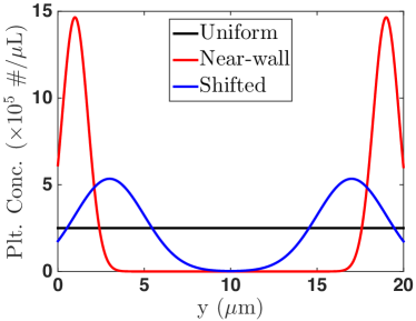
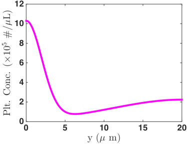
Figure 12: Upstream Platelet Distributions: (A)Uniform ($P^{up}(y)=P^{up,*}$), near-wall, and shifted upstream platelet distributions. These are motivated by in vivo [43] and in vitro [8, 9, 44, 50] observations. Additional details are found in [24].

Under both high and low shear conditions, aggregates simulated with the uniform platelet distribution are the slowest growing in both thickness and density (Figure 13 A-B). The use of a near-wall platelet distribution, which has the highest concentration of platelets closest to the walls, results in the fastest occlusion time of approximately 1.75 minutes. The shifted platelet distribution produced aggregates that occlude approximately 30-45 seconds slower. A similar trend is seen in the low shear conditions Figure 13 C-D, however occlusion times are longer. The results from these symmetric cases yield aggregates with varying thicknesses and densities, identifying the upstream platelet distribution $P^{up}(y)$ as a modifier of aggregate formation. Additionally, we were motivated to perform experiments that address the effects of asymmetric upstream platelet distribution on aggregate formation.

Figure 14 A-D show aggregate thicknesses and densities associated with the bottom (purple) and top (green) walls. We chose an asymmetric distribution found in Figure 12 B, where there is a greater concentration of platelets near the bottom wall of the injury channel. The aggregate grows asymmetrically in both thickness and density. In high shear (HS) conditions, the bottom aggregate region is thicker and denser after 1.25 minutes. There is, however, a significant increase in the density of the top aggregate after 1.25 minutes, resulting in a thin but dense top aggregate. Similar behavior is seen in results under low shear (LS) conditions, however, there is a delay. Therefore, the model is able to produce aggregates of different orientations, thicknesses and densities by varying model inputs such as upstream platelet distribution and flow conditions.

(A)	(B)

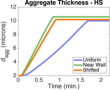
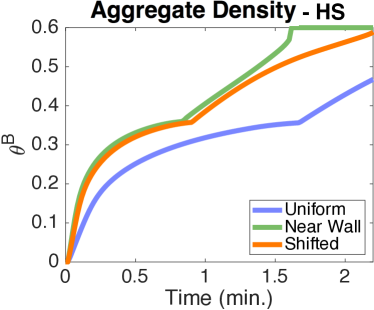
(C)	(D)

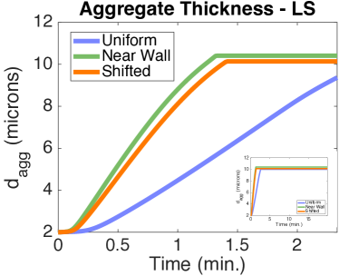
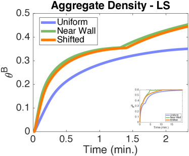
Figure 13: Symmetric Aggregate Formation: Given different symmetric upstream platelet distributions $P^{up}(y)$: uniform, near-wall, and shifted (see Figure 12A) with ADP-independent platelet activation $A([ADP]_{\text{agg}},[ADP]_{\text{BL}})=1$ under high shear (HS) conditions $(\gamma=2400\text{ s}^{-1}$) A) the aggregate thickness B) and density vary as functions of time. Similar comparisons under low shear (LS) conditions $(\gamma=100\text{ s}^{-1}$) yield aggregates of varying thickness (C) and density (D). Insets show results after 20 minutes of simulation time confirming occlusion.

(A)	(B)

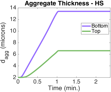
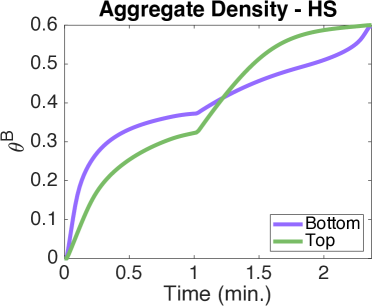
(C)	(D)

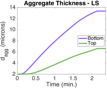
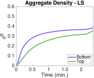
Figure 14: Asymmetric Aggregate Formation: Given an asymmetric upstream platelet distribution (see Figure 12B) with ADP-independent platelet activation ($A([ADP]_{\text{agg}},[ADP]_{\text{BL}})=1$) and high shear conditions ($\gamma=2400^{-1}$), the aggregate thickness A) and aggregate density B) as functions of time. Similar comparisons under low shear (LS) conditions $(\gamma=100\text{ s}^{-1}$) yield aggregates of varying thickness (C) and density (D).

References

- [1] H. Andersen, D. L. Greenberg, K. Fujikawa, W. Xu, D. W. Chung, and E. W. Davie, Protease-activated receptor 1 is the primary mediator of thrombin-stimulated platelet procoagulant activity, Proceedings of the National Academy of Sciences of the United States of America, 96 (1999), pp. 11189–93.
- [2] R. Andrews, M. Berndt, and J. Lopez, Platelets, Burlington: Academic, 2001, ch. The glycoprotein Ib-IX-V complex, pp. 145–163.
- [3] a. Baurand, P. Raboisson, M. Freund, C. Léon, J. P. Cazenave, J. J. Bourguignon, and C. Gachet, Inhibition of platelet function by administration of MRS2179, a P2Y1 receptor antagonist, European Journal of Pharmacology, 412 (2001), pp. 213–21.
- [4] K. Bledzka, S. S. Smyth, and E. F. Plow, Integrin : from discovery to efficacious therapeutic target, Circulation Research, 112 (2013), pp. 1189–1200.
- [5] T. V. Colace, R. W. Muthard, and S. L. Diamond, Thrombus growth and embolism on tissue factor-bearing collagen surfaces under flow: role of thrombin with and without fibrin, Arteriosclerosis, thrombosis, and vascular biology, 32 (2012), pp. 1466–1476.
- [6] E. L. Cussler, Diffusion Mass Transfer in Fluid Systems, Cambridge University Press, Cambridge, Third ed., 2009.
- [7] N. Danes and K. Leiderman, A density-dependent FEM-FCT algorithm with application to modeling platelet aggregation, International Journal for Numerical Methods in Biomedical Engineering, (2019), p. e3212.
- [8] E. C. Eckstein and F. Belgacem, Model of platelet transport in flowing blood with drift and diffusion terms, Biophysical Journal, 60 (1991), pp. 53–69.
- [9] E. C. Eckstein, A. W. Tilles, and F. J. Millero III, Conditions for the occurrence of large near-wall excesses of small particles during blood flow, Microvascular Research, 36 (1988), pp. 31–39.
- [10] P. Elizondo and A. L. Fogelson, A mathematical model of venous thrombosis initiation, Biophysical Journal, 111 (2016), pp. 2722–2734.
- [11] A. Fick, On liquid diffusion, The London, Edinburgh, and Dublin Philosophical Magazine and Journal of Science, 10 (1855), pp. 30–39.
- [12] A. L. Fogelson, Y. H. Hussain, and K. Leiderman, Blood Clot Formation under Flow : The Importance of Factor XI Depends Strongly on Platelet Count, Biophysical Journal, 102 (2012), pp. 10–18.
- [13] A. L. Fogelson and K. B. Neeves, Fluid mechanics of blood clot formation, Annual Review of Fluid Mechanics, 47 (2015), pp. 377–403.
- [14] A. L. Fogelson and K. B. Neeves, Fluid Mechanics of Blood Clot Formation, Annual Review of Fluid Mechanics, 47 (2015), pp. 377–403.
- [15] A. L. Fogelson and N. Tania, Coagulation under flow: The influence of flow-mediated transport on the initiation and inhibition of coagulation, Pathophysiology of Haemostasis and Thrombosis, 34 (2006), pp. 91–108.
- [16] A. R. Gear, Platelet adhesion, shape change, and aggregation: rapid initiation and signal transduction events, Canadian Journal of Physiology and Pharmacology, 72 (1994), pp. 285–294.
- [17] E. F. Grabowski, J. T. Franta, and P. Didisheim, Platelet aggregation in flowing blood in vitro. ii. dependence of aggregate growth rate on adp concentration and shear rate, Microvascular Research, 16 (1978), pp. 183–195.
- [18] B. Hechler and C. Gachet, P2 receptors and platelet function, Purinergic Signalling, 7 (2011), pp. 293–303.
- [19] S. P. Jackson, Review Article: The growing complexity of platelet aggregation, Blood, 109 (2007), pp. 5087–5096.
- [20] S. P. Jackson, W. S. Nesbitt, and S. Kulkarni, Signaling events underlying thrombus formation, Journal of Thrombosis and Haemostasis, 1 (2003), pp. 1602–1612.
- [21] C. KJ and C. Clemetson, Platelets, Burlington: Academic, 2007, ch. Platelet Receptors, pp. 201–213.
- [22] A. L. Kuharsky and A. L. Fogelson, Surface-Mediated Control of Blood Coagulation : The Role of Binding Site Densities and Platelet Deposition, Biophysical Journal, 80 (2001), pp. 1050–1074.
- [23] K. Leiderman, W. C. Chang, M. Ovanesov, and A. L. Fogelson, Synergy Between Tissue Factor and Exogenous Factor XIa in Initiating Coagulation, Arteriosclerosis, Thrombosis, and Vascular Biology, 36 (2016), pp. 2334–2345.
- [24] K. Leiderman and A. L. Fogelson, Grow with the flow: A spatial-temporal model of platelet deposition and blood coagulation under flow, Mathematical Medicine and Biology, 28 (2011), pp. 47–84.
- [25] K. Leiderman and A. L. Fogelson, The influence of hindered transport on the development of platelet thrombi under flow, Bulletin of mathematical biology, 75 (2013), pp. 1255–1283.
- [26] K. Leiderman and A. L. Fogelson, The Influence of Hindered Transport on the Development of Platelet Thrombi Under Flow, Bulletin of Mathematical Biology, 75 (2013), pp. 1255–1283.
- [27] Z. Li, M. K. Delaney, K. A. O’Brien, and X. Du, Signaling during platelet adhesion and activation, Arteriosclerosis, Thrombosis, and Vascular Biology, 30 (2010), pp. 2341–2349.
- [28] K. G. Link, M. T. Stobb, J. Di Paola, K. B. Neeves, A. L. Fogelson, S. S. Sindi, and K. Leiderman, A local and global sensitivity analysis of a mathematical model of coagulation and platelet deposition under flow, PLOS ONE, 13 (2018).
- [29] K. G. Link, M. T. Stobb, M. G. Sorrells, M. Bortot, K. Ruegg, M. J. Manco-Johnson, J. A. Di Paola, S. S. Sindi, A. L. Fogelson, K. Leiderman, et al., A mathematical model of coagulation under flow identifies factor v as a modifier of thrombin generation in hemophilia a, Journal of Thrombosis and Haemostasis, (2019).
- [30] W. McCabe, J. Smith, and P. Harriott, Unit Operations of Chemical Engineering, Civil Engineering, McGraw-Hill Education, 2005.
- [31] R. W. Muthard and S. L. Diamond, Blood clots are rapidly assembled hemodynamic sensors: flow arrest triggers intraluminal thrombus contraction, Arteriosclerosis, Thrombosis, and Vascular Biology, 32 (2012), pp. 2938–2945.
- [32] K. Nogami and M. Shima, Phenotypic heterogeneity of hemostasis in severe hemophilia, in Seminars in thrombosis and hemostasis, vol. 41, Thieme Medical Publishers, 2015, pp. 826–831.
- [33] P. Ohlmann, S. de Castro, G. G. Brown, C. Gachet, K. A. Jacobson, and T. K. Harden, Quantification of recombinant and platelet P2Y1receptors utilizing a [125I]-labeled high-affinity antagonist 2-iodo-N6-methyl-(N)-methanocarba-2’-deoxyadenosine-3′,5′-bisphosphate ([125I]MRS2500), Pharmacological Research, 62 (2010), pp. 344–351.
- [34] K. Rana and K. B. Neeves, Blood flow and mass transfer regulation of coagulation, Blood Reviews, 30 (2016), pp. 357–368.
- [35] Z. M. Ruggeri, Platelet adhesion under flow., Microcirculation (New York, N.Y. : 1994), 16 (2009), pp. 58–83.
- [36] Z. M. Ruggeri, J. a. Dent, and E. Saldívar, Contribution of distinct adhesive interactions to platelet aggregation in flowing blood., Blood, 94 (1999), pp. 172–8.
- [37] K. S. S. Kobayashi and D. N. Ku, Occlusive thrombus growth at high shear rates: comparison of whole blood and platelet rich plasma at constant pressure, J. Thromb. Haemost., 14 (2016), pp. 6–7.
- [38] B. Savage, F. Almus-Jacobs, and Z. M. Ruggeri, Specific synergy of multiple substrate-receptor interactions in platelet thrombus formation under flow, Cell, 94 (1998), pp. 657–666.
- [39] B. Savage, E. Saldívar, and Z. M. Ruggeri, Initiation of platelet adhesion by arrest onto fibrinogen or translocation on von willebrand factor, Cell, 84 (1996), pp. 289–297.
- [40] R. Schoeman, K. Rana, N. Danes, M. Lehmann, J. Di Paola, A. Fogelson, K. Leiderman, and K. Neeves, A microfluidic model of hemostasis sensitive to platelet function and coagulation, Cellular and Molecular Bioengineering, 10 (2017), pp. 3–15.
- [41] L. F. Shampine and M. W. Reichelt, The matlab ode suite, SIAM Journal on Scientific Computing, 18 (1997), pp. 1–22.
- [42] T. Skorczewski, L. C. Erickson, and A. L. Fogelson, Platelet motion near a vessel wall or thrombus surface in two-dimensional whole blood simulations, Biophysical journal, 104 (2013), pp. 1764–1772.
- [43] G. Tangelder, H. C. Teirlinck, D. W. Slaaf, and R. S. Reneman, Distribution of blood platelets flowing in arterioles, American Journal of Physiology-Heart and Circulatory Physiology, 248 (1985), pp. H318–H323.
- [44] A. W. Tilles and E. C. Eckstein, The near-wall excess of platelet-sized particles in blood flow: its dependence on hematocrit and wall shear rate, Microvascular Research, 33 (1987), pp. 211–223.
- [45] L. Timmermans, P. Minev, and F. Van De Vosse, An approximate projection scheme for incompressible flow using spectral elements, International journal for Numerical Methods in Fluids, 22 (1996), pp. 673–688.
- [46] V. T. Turitto and E. F. Leonard, Platelet adhesion to a spinning surface, ASAIO Journal, 18 (1972), pp. 348–354.
- [47] L. Valentino, Blood-induced joint disease: the pathophysiology of hemophilic arthropathy, Journal of Thrombosis and Haemostasis, 8 (2010), pp. 1895–1902.
- [48] H. H. Versteeg, J. W. M. Heemskerk, M. Levi, and P. H. Reitsma, New Fundamentals in Coagulation, Physiology Review, 93 (2013), pp. 327–358.
- [49] A. Wufsus, N. Macera, and K. Neeves, The hydraulic permeability of blood clots as a function of fibrin and platelet density, Biophysical Journal, 104 (2013), pp. 1812–1823.
- [50] C. Yeh, A. C. Calvez, and E. C. Eckstein, An estimated shape function for drift in a platelet-transport model, Biophysical Journal, 67 (1994), pp. 1252–1259.