KEK-TH-2195

Extremal 1/2 Calabi–Yau 3-folds and six-dimensional F-theory applications

Yusuke Kimura^1
1KEK Theory Center, Institute of Particle and Nuclear Studies, KEK,
1-1 Oho, Tsukuba, Ibaraki 305-0801, Japan
E-mail: kimurayu@post.kek.jp

1 Introduction

U(1) symmetry is important in realizing the grand unified theory (GUT) because the presence of a U(1) symmetry helps explain a few of the characteristic properties of GUT, such as the mass hierarchies of the quarks and leptons, and a suppression of the proton decay. In F-theory [1, 2, 3], information of U(1) gauge symmetry can be extracted from the geometry of the compactification space. F-theory is compactified on elliptic fibrations, and the modular parameter of the tori as fibers of the elliptic fibration is identified with axiodilaton, enabling the axiodilaton to exhibit $SL(2,\mathbb{Z})$ monodromy. The $SL(2,\mathbb{Z})$ symmetry possessed by type IIB superstrings is realized in a geometric manner in the formulation of F-theory.

A certain structure of elliptic fibration, a global section, relates directly to the U(1) gauge symmetry that forms in F-theory. When one can choose a point in every elliptic fiber of the fibration, and the chosen point can be moved throughout the base space of the fibration, a genus-one fibration having such a structure is said to admit a global section, yielding a copy of the base space inside the total space of the fibration. When an elliptic fibration has a global section, the set of global sections forms a group, which is known as the “Mordell–Weil group.” The rank of the Mordell–Weil group of an elliptic fibration, in the context of physics, is related to the U(1) gauge group; the rank yields the number of U(1) factors formed in F-theory on that elliptic fibration [3].

F-theory models on elliptic fibrations having a global section have been intensively studied, e.g., in [4, 5, 6, 7, 8, 9, 10, 11, 12, 13, 14, 15, 16, 17, 18, 19, 20, 21, 22, 23, 24, 25, 26, 27, 28, 29, 30, 31, 32, 33, 34, 35, 36, 37, 38, 39, 40]. U(1) gauge symmetry has also been investigated in F-theory.

In this study, we mainly focus on six-dimensional (6D) F-theory.

Elliptic Calabi–Yau 3-folds of various Mordell–Weil ranks have recently been constructed by taking double covers of certain class of rational elliptic 3-folds, which are referred to as “1/2 Calabi–Yau 3-folds” [37]. F-theory on this type of Calabi–Yau 3-folds yields 6D $N=1$ theories with various numbers of U(1) factors [37]. A general construction scheme of elliptically fibered Calabi–Yau 3-folds by taking double covers of “1/2 Calabi–Yau 3-folds” is discussed in [37], and some explicit examples of 1/2 Calabi–Yau 3-folds with specific singularity types and Calabi–Yau 3-folds obtained as their double covers are discussed in [37].

The aim of this study is to discuss a strategy to classify the singularity types of the elliptic Calabi–Yau 3-folds constructed as double covers of 1/2 Calabi–Yau 3-folds. This result translates, in string theoretic language, to non-Abelian gauge groups forming in 6D F-theory compactifications on them. Furthermore, this analysis yields a description of the singular fibers and sections of 1/2 Calabi–Yau 3-folds and Calabi–Yau 3-folds as double covers. Therefore, the analysis also directly relates to U(1) gauge groups and matter fields arising in 6D F-theory compactifications.

There are some obstacles to studying the singularities of 1/2 Calabi–Yau 3-folds. The 1/2 Calabi–Yau 3-folds were constructed as blow-ups of $\mathbb{P}^{3}$ at the intersection points of three quadrics [37]. When studying the singular fibers of the resulting 1/2 Calabi–Yau 3-folds without resolving the singularity, only two conics meeting in two points can be found, and this generally does not determine the types of singular fibers. Determining the types of singular fibers given the equations of three quadrics requires multiple stages of resolutions, which makes an analysis of the singular fibers difficult to achieve.

To resolve this difficulty in analyzing the singularity types of 1/2 Calabi–Yau 3-folds directly, we relate the problem of classifying the singularity types of the 1/2 Calabi–Yau 3-folds to those of quartic curves in $\mathbb{P}^{2}$ by considering the “projective duals.” An interesting mathematical result observed by Mukai in [57, 58, 59], when applied to the 1/2 Calabi–Yau 3-folds, reveals that the classification of the 1/2 Calabi–Yau 3-folds is actually equivalent to the classification of the singularity types of the quartic curves in $\mathbb{P}^{2}$. The singularity types of the 1/2 Calabi–Yau 3-folds and those of plane quartic curves are actually equivalent based on the notion of the “projective duality” [59]. Making use of this duality, the classification problem of the singularity types of 1/2 Calabi–Yau 3-folds, which appeared to be obscure and somewhat difficult, begins to become more transparent, enabling us to find a way to resolve the problem. By making use of this method, we classify the singularity types of the 1/2 Calabi–Yau 3-folds when the rank is maximal, and furthermore, through this approach the singular fibers are described in detail. Based on this analysis, the structures of the global sections are also described. The discussion of these are the main goals of this paper.

Because a singularity type of Calabi–Yau 3-fold as a double cover of the original 1/2 Calabi–Yau 3-fold is identical to the singularity type of the original Calabi–Yau 3-fold [37], the classification results of singularity type 1/2 Calabi–Yau 3-folds also yield a classification of the singularity types of the Calabi–Yau 3-folds as double covers. From the viewpoint of F-theory, these results yield the non-Abelian gauge groups forming on the 7-branes in the 6D F-theory on the Calabi–Yau 3-folds. When the classification scheme is applied to 1/2 Calabi–Yau 3-folds of singularity ranks of strictly lower than seven, by taking their double covers, 6D $N=1$ F-theory models with (multiple) U(1) factors can also be analyzed. Because our analysis here includes a description of the singular fibers, the analysis can also be applied to the matter spectra in the 6D compactifications.

Obtaining the Weierstrass equations of the 1/2 Calabi–Yau 3-folds can be considerably difficult as pointed out in [37]. Although obtaining the Weierstrass equations is useful in determining the gauge groups and the matter spectra, we take an approach to deduce the singularity types and the singular fibers directly from the defining equations of the three quadrics, which specify the complex structure of the 1/2 Calabi–Yau 3-fold described in this paper.

We focus on 1/2 Calabi–Yau 3-folds with a singularity rank of seven, which is the maximal rank for the 1/2 Calabi–Yau 3-folds [37], and we classify the singularity types of such 1/2 Calabi–Yau 3-folds in this study. We refer to 1/2 Calabi–Yau 3-folds having the maximal rank-seven singularity types as “extremal 1/2 Calabi–Yau 3-folds.” The rank-seven singularity types of the quartic curves in $\mathbb{P}^{2}$ were realized in [60] and the classification of the rank-seven singularities consists of six types [60]. These six types yield the singularity types of the extremal 1/2 Calabi–Yau 3-folds via applying the method in [57, 58, 59]. Our classification method also applies to 1/2 Calabi–Yau 3-folds having lower singularity ranks.

By analyzing the extremal 1/2 Calabi–Yau 3-folds, we demonstrate that the structures of the singular fibers and the global sections can be explicitly seen by conducting blow-ups. Among the classified singularity types of the extremal 1/2 Calabi–Yau 3-folds, we study in detail two singularity types to describe the singular fibers and sections. These two types require relatively shallow levels of blow-ups to understand the structures of the singular fibers. However, other singularity types require deeper levels of blow-ups, as mentioned in section 3.3, and our study suggests that through multiple stages of blow-ups the singular fibers can be described in manners similar to the two singularity types.

Local model buildings [61, 62, 63, 64] have been emphasized in recent studies on F-theory. The global aspects of the models, however, need to be studied to discuss issues of gravity and problems pertaining to the early universe. The global aspects of the compactification geometry are analyzed in this study.

Studies on geometric structures of elliptically fibered 3-folds can be found in [65, 66, 67].

This paper is structured as follows: We discuss a method for classifying the singularity types of 1/2 Calabi–Yau 3-folds in section 2.1. The maximal rank seven singularity types of 1/2 Calabi–Yau 3-folds are described in sections 2.2 through 2.7. There are six types of such singularities. Two of these singularity types are analyzed in detail in sections 3.1 and 3.2. We demonstrate that the singular fibers and sections can be described after eight blow-ups. We also mention the remaining rank seven singularity types in section 3.3. The F-theory application is discussed in section 4. Singularity types of 1/2 Calabi–Yau 3-folds of ranks lower than seven and U(1) factors in 6D F-theory are also mentioned. Concluding remarks and remaining problems are mentioned in section 5. Problems that are possibly related to the swampland conditions are also discussed. Reviews of recent progress of the swampland criteria can be found in [68, 69]. In [70, 71, 72], the authors discussed the notion of the swampland. A new consistency condition on 6D $N=1$ quantum gravity theories was recently discussed in [73]. The authors of [74, 75, 76, 77] discussed the possible combinations of distinct matter fields and gauge symmetries for quantum gravity theories in 6D with $N=1$ supersymmetry.

2 Singularity types of 1/2 Calabi–Yau 3-folds and projective duality

2.1 Method to deduce the equations of three quadrics of 1/2 Calabi–Yau 3-folds

The 1/2 Calabi–Yau 3-folds constructed in [37] are rational elliptic 3-folds obtained by blowing up $\mathbb{P}^{3}$ at the intersection points of three quadrics. The base surface of a 1/2 Calabi–Yau 3-fold is isomorphic to $\mathbb{P}^{2}$, and taking the ratio of three quadrics $q_{1},q_{2},q_{3}$, $[q_{1}:q_{2}:q_{3}]$, yields the projection. Taking double covers of the 1/2 Calabi–Yau 3-folds (ramified along appropriate degree 8 hypersurfaces) yields elliptically fibered Calabi–Yau 3-folds, F-theory compactifications upon which 6D $N=1$ theories are provided [37].

The singularity types of the original 1/2 Calabi–Yau 3-fold and the Calabi–Yau 3-fold as its double cover are identical [37], thus determining the singular fibers and the singularity types of the 1/2 Calabi–Yau 3-folds also determines the singularity types of elliptic Calabi–Yau 3-folds as double covers. This in principle determines the non-Abelian gauge symmetries that arise in F-theory on the Calabi–Yau 3-folds .

Pairs of algebraic varieties of different dimensions that are projective duals were studied in [59]. Applying the analysis in [59] to 1/2 Calabi–Yau 3-folds, the classifications of the singularity types of 1/2 Calabi–Yau 3-folds and the singularities of the quartic curves in $\mathbb{P}^{2}$ are found to be identical. Making use of this mathematical observation reduces the classification problem of the singularity types of 1/2 Calabi–Yau 3-folds to that of the singularities of the quartic curves in $\mathbb{P}^{2}$.

In [59], Mukai studied several pairs of del Pezzo manifolds, which are projective duals to each other. We apply one of these pairs, $(X_{2},Y_{8})$, to 1/2 Calabi–Yau 3-folds. Here, $X_{2}$ is a del Pezzo manifold of dimension ${\rm dim}_{\mathbb{C}}X_{2}=9$, and del Pezzo manifold $Y_{8}$ has dimensions of ${\rm dim}_{\mathbb{C}}Y_{8}=3$. $X_{2}$ is a double cover of $\mathbb{P}^{9}$ ramified over quartic hypersurface $D_{4}$, and $Y_{8}$ is the Veronese 3-fold $v_{2}(\mathbb{P}^{3})$ embedded inside $\mathbb{P}^{9}$ [59]. Moreover, $X_{2}$ and $Y_{8}$ are projective duals to each other [59]. Here, $X_{2}$ cut out by seven hyperplanes yields a double cover of $\mathbb{P}^{2}$ ramified over a quartic curve, which is the degree-two del Pezzo surface . Because the projective dual of a hyperplane is a point, the operation of cutting $X_{2}$ by seven hyperplanes on the $Y_{8}$ side corresponds to the choice of seven points. The seven points span $\mathbb{P}^{6}$, and therefore cutting $X_{2}$ by seven hyperplanes corresponds on the $Y_{8}$ side to taking the intersection of $Y_{8}=v_{2}(\mathbb{P}^{3})$ and $\mathbb{P}^{6}$ inside $\mathbb{P}^{9}$, $v_{2}(\mathbb{P}^{3})\cap\mathbb{P}^{6}\subset\mathbb{P}^{9}$. The intersection is equivalent to cutting $v_{2}(\mathbb{P}^{3})$ by three hyperplanes inside $\mathbb{P}^{9}$. Because $v_{2}(\mathbb{P}^{3})$ is a Veronese embedding of $\mathbb{P}^{3}$ into $\mathbb{P}^{9}$, taking the intersection $v_{2}(\mathbb{P}^{3})\cap\mathbb{P}^{6}\subset\mathbb{P}^{9}$ is equivalent to the intersection of the three quadrics in $\mathbb{P}^{3}$ [59]. $X_{2}$ cut out by seven hyperplanes is isomorphic to the degree-two del Pezzo surface [59] which is a double cover of $\mathbb{P}^{2}$ ramified over a quartic curve, and the blow-up of $\mathbb{P}^{3}$ at the intersection points of the three quadrics yields the Jacobian of the degree-two del Pezzo surface [57, 58, 59]. Therefore, the singularity types of the quartic curves in $\mathbb{P}^{2}$ are identical to the singularity types of the 1/2 Calabi–Yau 3-folds, and the correspondence is manifest through the projective duality discussed in [59].

To describe the correspondence of the equations of three quadrics of a 1/2 Calabi–Yau 3-fold and the quartic curve in $\mathbb{P}^{2}$, when the determinantal representation of a plane quartic curve is given as a symmetric 4 $\times$ 4 matrix, matrix elements correspond to the equations of the three quadrics in $\mathbb{P}^{3}$ via the method discussed in [57, 58, 59]. When one finds the determinantal representation of a quartic curve, equations of the three quadrics of the dual 1/2 Calabi–Yau 3-fold can be deduced from the determinantal representation.

The maximal singularity rank of 1/2 Calabi–Yau 3-folds is seven [37]. We classify the rank seven singularity types of the 1/2 Calabi–Yau 3-folds utilizing the method in [57, 58, 59]. The 1/2 Calabi–Yau 3-folds possessing the maximal rank seven singularity types are referred to as extremal 1/2 Calabi–Yau 3-folds in this note.

The classification of the singularity types of the quartic curves in $\mathbb{P}^{2}$ can be found in [60]. Among the singularities, seven is the maximal rank and there are six rank-seven singularity types [60]: $D_{4}A_{1}^{3}$, $A_{3}^{2}A_{1}$, $A_{5}A_{2}$, $A_{7}$, $D_{6}A_{1}$, $E_{7}$. Therefore, from the argument given, we found that the extremal 1/2 Calabi–Yau 3-folds have six singularity types via applying the method in [57, 58, 59]. The corresponding six singularity types of the plane quartics are shown in Figures 1, 2, and 3.

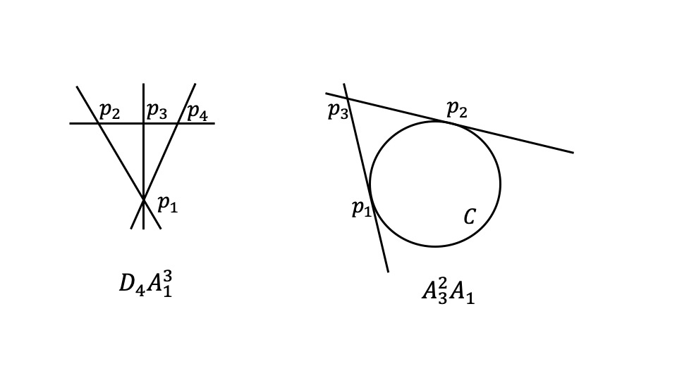
Figure 1: The left image describes the quartic curve, which is reducible into three lines meeting at one point and a line. This curve has $D_{4}A_{1}^{3}$ singularity [60]. The point at which three lines simultaneously meet yields a $D_{4}$ singularity, and each of the other three intersection points yields $A_{1}$ singularity. The right image describes a quartic curve reducible into one conic and two tangents. The quartic curve on the right has $A_{3}^{2}A_{1}$ singularity [60]. Two points at which two lines are tangent to the conic yield two $A_{3}$ singularities. The intersection of two lines yields $A_{1}$ singularity.

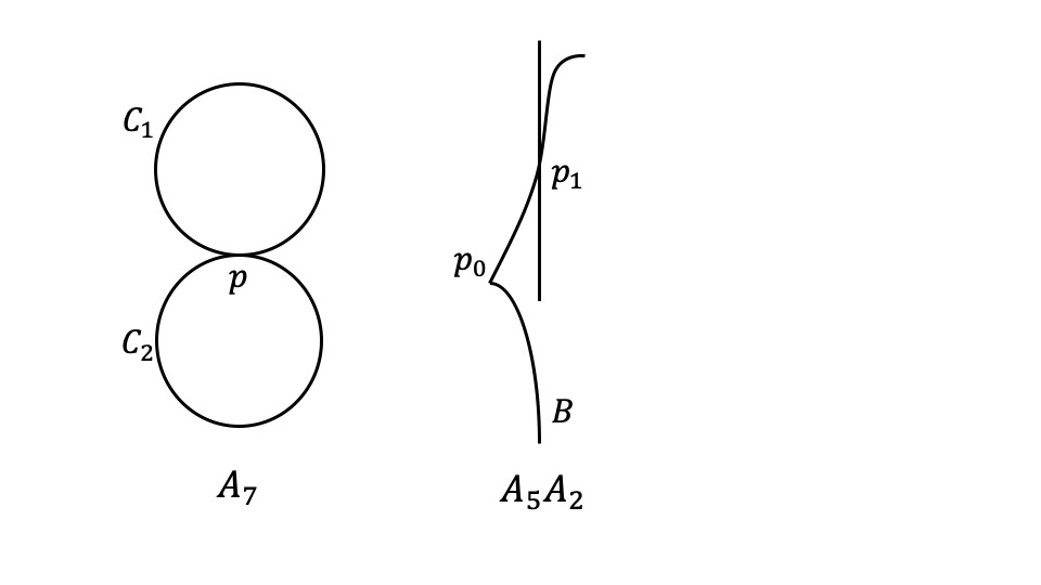
Figure 2: The left image describes a quartic curve reducible into two conics meeting at a point. The left quartic curve has $A_{7}$ singularity [60]. The intersection point yields $A_{7}$ singularity. The right image describes a cubic with a cusp and a line tangent to the flex. The quartic curve on the right has $A_{5}A_{2}$ singularity [60]. A cusp yields $A_{2}$ singularity, and the tangent point of the flex and the line yields $A_{5}$ singularity.

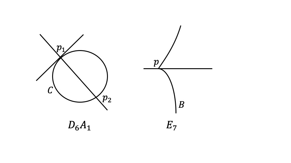
Figure 3: The left image describes a quartic curve reducible into a conic, a line tangent to the conic, and another line through the tangent point. The left quartic curve has $D_{6}A_{1}$ singularity [60]. The right image is a cubic with a cusp and cuspidal tangent. The right quartic curve has $E_{7}$ singularity [60].

As presented in Figures 1, 2, and 3, the quartic curves with rank seven singularities are reducible into a cubic and a line, two conics, lines and a conic, or four lines. Considering their determinantal representations, these situations correspond to a 4 $\times$ 4 matrix reducible into smaller blocks of submatrices.

Given the series of observations, we are now ready to deduce the equations of the three quadrics of the extremal 1/2 Calabi–Yau 3-folds, which are described in sections 2.2, 2.3, 2.4, 2.5, 2.6, and 2.7.

2.2 $D_{4}A_{1}^{3}$ singularity

We determine the equations of the three quadrics yielding the extremal 1/2 Calabi–Yau 3-fold with the singularity type $D_{4}A_{1}^{3}$, when $\mathbb{P}^{3}$ is blown up at the intersections of the three quadrics.

The dual quartic curve with the $D_{4}A_{1}^{3}$ singularity is the sum of three lines meeting at a point and a line [60], as presented in Figure 1. This quartic curve is given by the following equation:

$$\lambda(\lambda-\mu)\mu\nu=0,$$ (1)

where $[\lambda:\mu:\nu]$ denotes the coordinates of $\mathbb{P}^{2}$. The three lines $\lambda=0$, $\mu=0$, and $\lambda-\mu=0$ yield three lines meeting at a point, which we denote as $p_{1}$. The determinantal representation of the quartic curve (1) is given as follows:

$$\begin{pmatrix}\lambda&0&0&0\\ 0&\mu-\lambda&0&0\\ 0&0&-\mu&0\\ 0&0&0&\nu\end{pmatrix}.$$ (2)

The equations of the three quadrics, $q_{1},q_{2},q_{3}$, can be deduced from the determinantal representation (2). The entries of the matrix (2) where $\lambda$ appears yield the coefficients of the quadric $q_{1}$, the entries where $\mu$ appears yield the coefficients of the quadric $q_{2}$, and the entries where $\nu$ appears give the coefficients of the quadric $q_{3}$. For example, the variable $\lambda$ appears in the (1, 1) and (2, 2) entries of matrix (2). Because the coefficient of $\lambda$ in the (1, 1) entry is 1 and the coefficient of $\lambda$ in the (2, 2) entry is $-1$, the equation of the quadric $q_{1}$ is given as $x^{2}-y^{2}$ (where the (1, 1) entry corresponds to $x^{2}$, and the (2, 2) entry corresponds to $y^{2}$). Here, $[x:y:z:w]$ denotes the coordinates of $\mathbb{P}^{3}$ (the blow-up of which yields a 1/2 Calabi–Yau 3-fold). The equations of the remaining two quadrics $q_{2},q_{3}$ are determined in a similar fashion. The equations of the three quadrics are determined as follows:

$$q_{1}= x^{2}-y^{2}$$ (3)

$$q_{2}= y^{2}-z^{2}$$

$$q_{3}= w^{2}.$$

We denote the curve in the base surface $\mathbb{P}^{2}$ of the 1/2 Calabi–Yau 3-fold dual to the $D_{4}$ singularity $p_{1}=[0:0:1]$ of the quartic (1) by $l_{1}$. Here, $l_{1}$ is given by $c=0$ in the base $\mathbb{P}^{2}$, where we use $[a:b:c]$ to denote the homogeneous coordinates of the base $\mathbb{P}^{2}$ of the 1/2 Calabi–Yau 3-folds. We denote by $l_{2},l_{3},l_{4}$ the three curves dual to the three intersection points, $p_{2},p_{3},p_{4}$, of the curve $\nu=0$ with each of the three curves $\lambda=0,\mu=0$, and $\lambda=\mu$ yielding $A_{1}$ singularities. The discriminant of the extremal 1/2 Calabi–Yau 3-fold with $D_{4}A_{1}^{3}$ singularity given by blowing up the base points of the three quadrics (3) is then given by the following:

$$\Delta\sim l_{1}^{6}\cdot l_{2}^{2}\cdot l_{3}^{2}\cdot l_{4}^{2}.$$ (4)

2.3 $A_{3}^{2}A_{1}$ singularity

We deduce the three quadrics yielding the extremal 1/2 Calabi–Yau 3-fold with an $A_{3}^{2}A_{1}$ singularity type. The plane quartic curve with $A_{3}^{2}A_{1}$ singularity is reducible into a conic and two lines tangent to it, as presented in Figure 1. The equation of the quartic curve is as follows:

$$(\mu\nu-\lambda^{2})\mu\nu=0,$$ (5)

and the determinantal representation is reducible into two linear factors and a 2 $\times$ 2 submatrix. The determinantal representation is given as follows:

$$\begin{pmatrix}\mu&\lambda&0&0\\ \lambda&\nu&0&0\\ 0&0&-\mu&0\\ 0&0&0&-\nu\end{pmatrix}.$$ (6)

The equations of the three quadrics can be deduced from the representation (6) in a way similar to that discussed in section 2.2, and the three quadrics are given as follows:

$$q_{1}= 2xy$$ (7)

$$q_{2}= x^{2}-z^{2}$$

$$q_{3}= y^{2}-w^{2}.$$

We denote the conic $\mu\nu-\lambda^{2}=0$ as $C$, and use $C^{*}$ to denote the dual curve of $C$ in the base $\mathbb{P}^{2}$. We denote the curves in the base $\mathbb{P}^{2}$ of the 1/2 Calabi–Yau 3-fold dual to the two points $p_{1}=[0:0:1],p_{2}=[0:1:0]$ at which each of the two lines $\mu=0,\nu=0$ is tangent to the conic $C$ yielding $A_{3}$ singularities by $l_{1},l_{2}$. $l_{1}$ is given by $c=0$, and $l_{2}$ is given by $b=0$. The curve dual to the intersection point $p_{3}$ of the two lines yielding an $A_{1}$ singularity is denoted as $l_{3}$. The extremal 1/2 Calabi–Yau 3-fold with an $A_{3}^{2}A_{1}$ singularity type then has the following discriminant:

$$\Delta\sim C^{*}\cdot l_{1}^{4}\cdot l_{2}^{4}\cdot l_{3}^{2}.$$ (8)

2.4 $A_{7}$ singularity

We deduce the equations of the three quadrics yielding the extremal 1/2 Calabi–Yau 3-folds with $A_{7}$ singularity. The quartic curve in $\mathbb{P}^{2}$ possessing $A_{7}$ singularity is two conics meeting at one point, as presented in Figure 2. The equation of this quartic curve is given as follows:

$$(\lambda\nu-\mu^{2})\big{(}\lambda(\lambda+\nu)-\mu^{2}\big{)}=0.$$ (9)

The determinantal representation of the quartic curve is given in the following:

$$\begin{pmatrix}\lambda&\mu&0&0\\ \mu&\nu&0&0\\ 0&0&\lambda&\mu\\ 0&0&\mu&\lambda+\nu\end{pmatrix}.$$ (10)

The equations of the three quadrics can be deduced from the representation (10), and the three quadrics are given as follows:

$$q_{1}= x^{2}+z^{2}+w^{2}$$ (11)

$$q_{2}= 2xy+2zw$$

$$q_{3}= y^{2}+w^{2}.$$

We denote the two conics of the quartic curve (9) by $C_{1}$ and $C_{2}$. The curve in the base $\mathbb{P}^{2}$ of the 1/2 Calabi–Yau 3-fold dual to the intersection point $p=[0:0:1]$ of the two conics $C_{1}$ and $C_{2}$ is given by $c=0$. We denote this dual curve in the base $\mathbb{P}^{2}$ by $l$, and denote the duals of the conics $C_{1}$ and $C_{2}$ by $C_{1}^{*}$ and $C_{2}^{*}$, respectively. The discriminant of the extremal 1/2 Calabi–Yau 3-fold with an $A_{7}$ singularity type is then given as follows:

$$\Delta\sim l^{8}\cdot C_{1}^{*}\cdot C_{2}^{*}.$$ (12)

2.5 $A_{5}A_{2}$ singularity

We determine the equations of the three quadrics yielding the extremal 1/2 Calabi–Yau 3-folds with $A_{5}A_{2}$ singularity. The plane quartic curve possessing $A_{5}A_{2}$ singularity is a cubic curve with a cusp and a line tangent to the flex, as presented in Figure 2. The equation of this quartic curve is given as follows:

$$(\lambda^{3}+\mu\nu^{2})\mu=0.$$ (13)

The determinantal representation of the quartic curve is given in the following:

$$\begin{pmatrix}-\mu&0&\lambda&0\\ 0&-\lambda&\nu&0\\ \lambda&\nu&0&0\\ 0&0&0&\mu\end{pmatrix}.$$ (14)

The equations of the three quadrics are obtained from the representation (14), and the three quadrics are given as follows:

$$q_{1}= -y^{2}+2xz$$ (15)

$$q_{2}= -x^{2}+w^{2}$$

$$q_{3}= 2yz.$$

The curve in the base $\mathbb{P}^{2}$ of the 1/2 Calabi–Yau 3-fold dual to the cusp $p_{0}=[0:1:0]$ of the cuspidal cubic in (13) yielding $A_{2}$ singularity is given by $b=0$, and we denote this curve in the base $\mathbb{P}^{2}$ by $l_{0}$. The cuspidal cubic $\lambda^{3}+\mu\nu^{2}=0$ in (13) is denoted as $B$, and the dual curve in the base $\mathbb{P}^{2}$ is denoted as $B^{*}$. The curve in the base $\mathbb{P}^{2}$ dual to the flex $p_{1}=[0:0:1]$ in the cuspidal cubic $B$ yielding an $A_{5}$ singularity is given by $c=0$ in the base; we denote this curve in the base $\mathbb{P}^{2}$ as $l_{1}$. The discriminant of the extremal 1/2 Calabi–Yau 3-fold is then given by the following:

$$\Delta\sim l_{0}^{3}\cdot l_{1}^{6}\cdot B^{*}.$$ (16)

2.6 $D_{6}A_{1}$ singularity

We determine the equations of the three quadrics yielding extremal 1/2 Calabi–Yau 3-folds with $D_{6}A_{1}$ singularity. The quartic curve in $\mathbb{P}^{2}$ possessing $D_{6}A_{1}$ singularity is a conic and a tangent line to it, and another line passing through the tangent point, as presented in Figure 3. The equation of this quartic curve is given as follows:

$$(\lambda\nu-\mu^{2})\lambda\mu=0.$$ (17)

The determinantal representation of the quartic curve is given in the following:

$$\begin{pmatrix}\lambda&\mu&0&0\\ \mu&\nu&0&0\\ 0&0&\lambda&0\\ 0&0&0&\mu\end{pmatrix}.$$ (18)

The equations of the three quadrics are deduced from the representation (18), and the three quadrics are given as follows:

$$q_{1}= x^{2}+z^{2}$$ (19)

$$q_{2}= w^{2}+2xy$$

$$q_{3}= y^{2}.$$

The conic $\lambda\nu-\mu^{2}=0$ in the quartic (17) is denoted as $C$. We denote by $l_{1}$ the curve in the base $\mathbb{P}^{2}$ of the 1/2 Calabi–Yau 3-fold dual to point $p_{1}$ at which the line $\lambda=0$ is tangent to the conic $C$ yielding $D_{6}$ singularity. We denote by $l_{2}$ the curve in the base $\mathbb{P}^{2}$ dual to the intersection $p_{2}$ of the line $\mu=0$ and the conic $C$ yielding $A_{1}$ singularity. The discriminant of the extremal 1/2 Calabi–Yau 3-fold with $D_{6}A_{1}$ singularity type is then given by the following:

$$\Delta\sim l_{1}^{8}\cdot l_{2}^{2}\cdot C^{*}.$$ (20)

2.7 $E_{7}$ singularity

We determine the equations of the three quadrics yielding the extremal 1/2 Calabi–Yau 3-folds with the $E_{7}$ singularity type. The quartic curve in $\mathbb{P}^{2}$ possessing the $E_{7}$ singularity type is a cubic with a cusp and the cuspidal tangent, as presented in Figure 3. The equation of this quartic curve is given as follows:

$$(\lambda^{3}+\mu\nu^{2})\nu=0.$$ (21)

The determinantal representation of the quartic curve is given in the following:

$$\begin{pmatrix}-\mu&0&\lambda&0\\ 0&-\lambda&\nu&0\\ \lambda&\nu&0&0\\ 0&0&0&\nu\end{pmatrix}.$$ (22)

The equations of the three quadrics are deduced from the representation (22), and the three quadrics are given as follows:

$$q_{1}= -y^{2}+2xz$$ (23)

$$q_{2}= -x^{2}$$

$$q_{3}= 2yz+w^{2}.$$

The cuspidal cubic $\lambda^{3}+\mu\nu^{2}=0$ in (21) is denoted as $B$. The curve in the base surface $\mathbb{P}^{2}$ of the 1/2 Calabi–Yau 3-fold dual to the $E_{7}$ singularity at the cusp $p=[0:1:0]$ of the cuspidal cubic $B$ is denoted as $l$; in addition, the curve $l$ is given by $b=0$. The discriminant of the extremal 1/2 Calabi–Yau 3-fold with singularity type $E_{7}$ is then given as follows:

$$\Delta\sim l^{9}\cdot B^{*}.$$ (24)

3 Singular fibers of extremal 1/2 Calabi–Yau 3-fold

Studying the equations of the three quadrics of the extremal 1/2 Calabi–Yau 3-folds, we analyze the singular fibers. We perform operations of blow-ups to conduct this analysis. The extremal 1/2 Calabi–Yau 3-folds with the singularity types $D_{4}A_{1}^{3}$ and $A_{3}^{2}A_{1}$ require only shallow levels of blow-ups to understand the structures of the singular fibers and sections. The results of the blow-ups of the two singularity types are described in sections 3.1 and 3.2. While the remaining four types of singularities require deeper levels of blow-ups, the singular fibers and sections are expected to be understood in a similar fashion. We discuss these cases in section 3.3.

3.1 Extremal 1/2 Calabi–Yau 3-fold with $D_{4}A_{1}^{3}$ singularity

We study the three quadrics yielding the 1/2 Calabi–Yau 3-fold with the $D_{4}A_{1}^{3}$ singularity deduced in section 2.2 to demonstrate that this extremal 1/2 Calabi–Yau 3-fold has type $I_{0}^{*}$ fibers.

From the equations of the three quadrics (3), we can see that there are four base points: $[1:\pm 1:\pm 1:0]$. Because there are generally eight base points given three quadrics, this result implies that each of the four base points has multiplicity 2. This can also be viewed as four points and an additional four points “ infinitely near” to them.

Blowing up the four base points $[1:\pm 1:\pm 1:0]$ separates the four points and the four points infinitely near to them. From the equations of the three quadrics, we can see that the singular fiber corresponding to the $D_{4}$ singularity is

$$b(x^{2}-y^{2})-a(y^{2}-z^{2})= 0$$ (25)

$$w^{2}= 0,$$

where $a,b$ denote parameters such that $[a:b]$ parameterizes the discriminant component. The equation (25) represents a double conic. Because the double conic (25) contains the four base points, when the four base points are blown up, four $\mathbb{P}^{1}$s arise from the four base points in the double conic. As a result of the four blow-ups, the singular fiber corresponding to $D_{4}$ singularity is described as a conic and four $\mathbb{P}^{1}$s, each of which intersects with the conic in one point. Therefore, we can explicitly see that, after the four blow-ups, type $I_{0}^{*}$ fibers appear. This situation is shown in Figure 4.

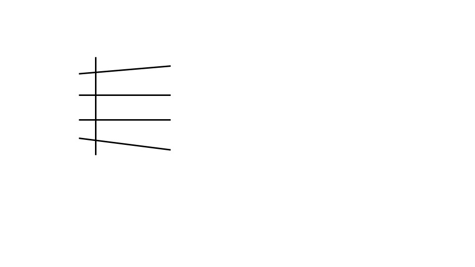
Figure 4: The image shows a singular fiber corresponding to $D_{4}$ singularity. The vertical line represents a conic, and the four horizontal lines represent $\mathbb{P}^{1}$s that result from the initial four blow-ups. This describes a type $I_{0}^{*}$ fiber.

When the total space $\mathbb{P}^{3}$ is considered, after these four blow-ups occur at the four base points, four $\mathbb{P}^{2}$s arise. Each of the $\mathbb{P}^{2}$s contains one point of indeterminacy. The morphism from each $\mathbb{P}^{2}$ arising from the blow-ups to the base $\mathbb{P}^{2}$ is not a surjection, and the image is isomorphic to $\mathbb{P}^{1}$. We consider the blow-ups of the four points of indeterminacy. These additional four blow-ups transform the four $\mathbb{P}^{2}$s that appeared from the previous four blow-ups into Hirzebruch surface $\mathbb{F}_{1}$s, and $\mathbb{P}^{2}$ arises from each of the four $\mathbb{F}_{1}$s. Each of the four $\mathbb{P}^{2}$s that arose from the latter four blow-ups surjects onto the base $\mathbb{P}^{2}$ under the projection. They yield sections and generate the Mordell–Weil group.

3.2 Extremal 1/2 Calabi–Yau 3-fold with $A_{3}^{2}A_{1}$ singularity

Next, we analyze the singular fibers of the extremal 1/2 Calabi–Yau 3-fold with the $A_{3}^{2}A_{1}$ singularity type by conducting a blow-up. The base points of the three quadrics (7) consist of four points: $[0:1:0:\pm 1]$, $[1:0:\pm 1:0]$. The singular fibers corresponding to one of the two $A_{3}$ singularities are given by the following:

$$2b\,xy-a(x^{2}-z^{2})= 0$$ (26)

$$y^{2}-w^{2}= 0,$$

($[a:b]$ parameterizes the discriminant component.) The result of the singular fibers corresponding to the other $A_{3}$ singularity is analogous to what we now describe. Without a blow-up, (because $y^{2}-w^{2}=0$ in (26) splits into two linear factors,) one can only find two conics intersecting at two points, and the type $I_{4}$ fiber is not apparent.

The two conics in (26) intersect at two points $[1:0:\pm 1:0]$, which are two among the base points. When these points are blown up, two intersecting conics are separated as a result of the two blow-ups, and two $\mathbb{P}^{1}$s arise from the two intersection points. Consequently, the structure of the type $I_{4}$ fibers becomes clear after the two blow-ups, as described in Figure 5. When the remaining two base points $[0:1:0:\pm 1]$ are blown up, the structure of the type $I_{4}$ fibers can also be explicitly seen from the other $A_{3}$ singularity.

Figure 5: The left image represents two conics meeting at two points before the blow-ups. The right image describes type $I_{4}$ fiber after two blow-ups. The two vertical lines are two separated conics, and the horizontal blue lines are two $\mathbb{P}^{1}$s that arise after two blow-ups.

When conducting four blow-ups of the four points, four $\mathbb{P}^{2}$s arise from the total space $\mathbb{P}^{3}$. When four additional blow-ups of the resulting $\mathbb{P}^{2}$s are applied, these latter four blow-ups transform the four $\mathbb{P}^{2}$s that arise from the previous four blow-ups into four $\mathbb{F}_{1}$s, and the four $\mathbb{P}^{2}$s that arise from the latter four blow-ups surject onto $\mathbb{P}^{2}$ through projection, yielding global sections, generating the Mordell–Weil group.

3.3 Extremal 1/2 Calabi–Yau 3-folds with other singularity types

Extremal 1/2 Calabi–Yau 3-folds with the other four singularity types require deeper levels of blow-ups to analyze the singular fibers. The extremal 1/2 Calabi–Yau 3-folds with two singularity types discussed in sections 3.1 and 3.2 required two stages of blow-ups: the first four blow-ups and the next four blow-ups. After these blow-ups, the structures of the singular fibers and sections can clearly be seen.

For example, concerning the extremal 1/2 Calabi–Yau 3-folds with $A_{7}$ and $A_{5}A_{2}$ singularities before a blow-up, only two conics meeting at two points can be seen from the $A_{7}$ and $A_{5}$ singularities. The base points of the quadrics yielding extremal 1/2 Calabi–Yau 3-folds with the two singularities $A_{7}$ and $A_{5}A_{2}$ consist of two and three points, respectively, implying that extremal 1/2 Calabi–Yau 3-folds with $A_{7}$ and $A_{5}A_{2}$ singularities require deeper stages of blow-ups to analyze the singular fibers than those described in sections 3.1 and 3.2. It is expected that, after multiple stages of blow-ups, $\mathbb{P}^{1}$s forming an octagon and hexagon can be seen from $A_{7}$ and $A_{5}$ singularities, yielding type $I_{8}$ and $I_{6}$ fibers.

For extremal 1/2 Calabi–Yau 3-folds with $D_{6}A_{1}$ and $E_{7}$ singularities, after multiple stages of blow-ups, we expect that type $I_{2}^{*}$ and type $III^{*}$ fibers can be explicitly seen from the $D_{6}$ and $E_{7}$ singularities. A future study can focus on investigating the detailed structures of extremal 1/2 Calabi–Yau 3-folds with these singularity types.

4 Application to 6D F-theory

Taking double covers of 1/2 Calabi–Yau 3-folds ramified over a hypersurface of degree 4 in terms of the three quadrics $q_{1},q_{2},q_{3}$ yields elliptic Calabi–Yau 3-folds [37]. Seven tensor fields arise in 6D $N=1$ F-theory on the resulting Calabi–Yau 3-folds [37]. The resulting Calabi–Yau 3-fold and the original 1/2 Calabi–Yau 3-fold have an identical singularity type [37]. Therefore, taking double covers of the extremal 1/2 Calabi–Yau 3-folds yields elliptic Calabi–Yau 3-folds with singularity types $E_{7}$, $D_{6}A_{1}$, $A_{7}$, $A_{5}A_{2}$, $A_{3}^{2}A_{1}$, and $D_{4}A_{1}^{3}$. $E_{7}$ gauge group forms in 6D F-theory on the Calabi–Yau 3-fold obtained as double cover of 1/2 Calabi–Yau 3-fold with $E_{7}$ singularity type as constructed in section 2.7.

The sum of the Mordell–Weil rank and the rank of the singularity type of a 1/2 Calabi–Yau 3-fold is always seven [37], and therefore every extremal 1/2 Calabi–Yau 3-fold has Mordell–Weil rank 0. A Calabi–Yau 3-fold as a double cover of an extremal 1/2 Calabi–Yau 3-fold has Mordell–Weil rank equal to or greater than the extremal 1/2 Calabi–Yau 3-fold [37], and thus not much can be stated regarding the U(1) symmetry forming in 6D F-theory on the resulting Calabi–Yau 3-folds constructed as double covers of extremal 1/2 Calabi–Yau 3-folds.

The method relating the singularity types of 1/2 Calabi–Yau 3-folds to those of the quartic curves in $\mathbb{P}^{2}$ discussed in section 2.1 also applies to 1/2 Calabi–Yau 3-folds of lower singularity ranks. Thus, we obtain the classification of the singularity types of 1/2 Calabi–Yau 3-folds from the classification results of the plane quartic curves [60], by applying the method in [57, 58, 59]. Concrete constructions of the subextremal 1/2 Calabi–Yau 3-folds (namely 1/2 Calabi–Yau 3-folds possessing the singularity types of rank 6) can be a likely target of future studies. Because the subextremal 1/2 Calabi–Yau 3-folds have Mordell–Weil rank 1, their double covers yield Calabi–Yau 3-folds of Mordell–Weil rank of at least 1. 6D $N=1$ F-theory compactifications on the resulting Calabi–Yau 3-folds have (at least) one U(1) factor.

We utilized the “duality” of the singularities of the quartic curves in $\mathbb{P}^{2}$ and the 1/2 Calabi–Yau 3-folds to deduce the equations of the three quadrics yielding the extremal 1/2 Calabi–Yau 3-folds. The discriminant of a Calabi–Yau 3-fold constructed as a double cover of a 1/2 Calabi–Yau 3-fold can be deduced from the discriminant of the 1/2 Calabi–Yau 3-fold [37]. The discriminants of the extremal 1/2 Calabi–Yau 3-folds were deduced in sections 2.2 - 2.7 by utilizing the duality of the singularity types of the plane quartic curves and the 1/2 Calabi–Yau 3-folds. This method also applies to 1/2 Calabi–Yau 3-folds of lower singularity ranks; therefore, the discriminants of the elliptic Calabi–Yau 3-folds as their double covers can also be deduced in a similar manner. Because matter fields localize at the intersections of the 7-branes wrapped on the discriminant components, the locations of the localized matter in 6D F-theory on the Calabi–Yau 3-folds are determined from the deduced discriminants. The base change lifts the global sections of the 1/2 Calabi–Yau 3-folds to sections of the Calabi–Yau 3-fold as their double covers [37].

Because the structures of the singular fibers can be analyzed through blow-up operations as demonstrated in sections 3.1 and 3.2, there is a chance that the matter spectra in 6D F-theory on the Calabi–Yau 3-folds can also be deduced by studying the structures of the singular fibers at the collisions of the fibers, which correspond to the intersections of the 7-branes, an investigation into which can be a direction of future study. Because the blow-up methods described in sections 3.1 and 3.2 revealed the structures of the sections, they might be used to analyze the explicit forms of the sections. The data mentioned can be used to determine the charges of the hypermultiplets charged under the $U(1)$ gauge symmetries [37], when 6D F-theory is compactified on Calabi–Yau 3-folds of positive Mordell–Weil ranks constructed as double covers of 1/2 Calabi–Yau 3-folds.

5 Open problems

We determined the singularity types of extremal 1/2 Calabi–Yau 3-folds, i.e., 1/2 Calabi–Yau 3-folds with a singularity of rank 7, and deduced the equations of the three quadrics yielding the extremal 1/2 Calabi–Yau 3-folds. Double covers of the extremal 1/2 Calabi–Yau 3-folds give elliptic Calabi–Yau 3-folds, the singularity types of which are identical to those of the original 1/2 Calabi–Yau 3-folds [37]. The methods we described in sections 3.1 and 3.2 enabled us to analyze the geometric structures of the singular fibers and sections. These methods might also have applications in investigating the matter fields arising in 6D F-theory on the Calabi–Yau 3-folds as double covers.

Seven tensor fields arise in 6D $N=1$ F-theory on elliptic Calabi–Yau 3-folds as double covers of 1/2 Calabi–Yau 3-folds [37]. The analysis in [37] suggests that 6D F-theory models with $T=7$ on Calabi–Yau 3-folds as double covers of 1/2 Calabi–Yau 3-folds are contained in vast numbers of models of 6D F-theory with $T=7$, based on the fact that non-Abelian gauge groups of ranks of up to only 7 can form in 6D F-theory on Calabi–Yau 3-folds as double covers of 1/2 Calabi–Yau 3-folds. Analogous to the fact that the points in the moduli of elliptic K3 surfaces where a K3 surface splits into a pair of rational elliptic surfaces correspond to the stable degeneration limit [80, 81] at which F-theory/heterotic duality [1, 2, 3, 82, 80] is strictly formulated, do the points in the complex structure moduli of Calabi–Yau 3-folds where a Calabi–Yau 3-fold splits into 1/2 Calabi–Yau 3-folds correspond to certain limits with a physical significance?

Furthermore, do elliptic Calabi–Yau 3-folds 6D F-theory compactifications on which have a number of tensor fields other than seven exhibit an analogous geometric structure wherein Calabi–Yau 3-folds allow splitting into building blocks of elliptic 3-folds? If so, investigating such elliptic Calabi–Yau 3-folds can be an interesting approach. If such Calabi–Yau 3-folds do not exist, do the 6D $N=1$ models with seven tensor fields have a special meaning? Investigating these questions might be interesting in relation to the swampland conditions.

References

- [1] C. Vafa, “Evidence for F-theory”, Nucl. Phys. B 469 (1996) 403 [arXiv:hep-th/9602022].
- [2] D. R. Morrison and C. Vafa, “Compactifications of F-theory on Calabi-Yau threefolds. 1”, Nucl. Phys. B 473 (1996) 74 [arXiv:hep-th/9602114].
- [3] D. R. Morrison and C. Vafa, “Compactifications of F-theory on Calabi-Yau threefolds. 2”, Nucl. Phys. B 476 (1996) 437 [arXiv:hep-th/9603161].
- [4] D. R. Morrison and D. S. Park, “F-Theory and the Mordell-Weil Group of Elliptically-Fibered Calabi-Yau Threefolds”, JHEP 10 (2012) 128 [arXiv:1208.2695 [hep-th]].
- [5] C. Mayrhofer, E. Palti and T. Weigand, “U(1) symmetries in F-theory GUTs with multiple sections”, JHEP 03 (2013) 098 [arXiv:1211.6742 [hep-th]].
- [6] V. Braun, T. W. Grimm and J. Keitel, “New Global F-theory GUTs with U(1) symmetries”, JHEP 09 (2013) 154 [arXiv:1302.1854 [hep-th]].
- [7] J. Borchmann, C. Mayrhofer, E. Palti and T. Weigand, “Elliptic fibrations for F-theory vacua”, Phys. Rev. D88 (2013) no.4 046005 [arXiv:1303.5054 [hep-th]].
- [8] M. Cvetič, D. Klevers and H. Piragua, “F-Theory Compactifications with Multiple U(1)-Factors: Constructing Elliptic Fibrations with Rational Sections”, JHEP 06 (2013) 067 [arXiv:1303.6970 [hep-th]].
- [9] V. Braun, T. W. Grimm and J. Keitel, “Geometric Engineering in Toric F-Theory and GUTs with U(1) Gauge Factors,” JHEP 12 (2013) 069 [arXiv:1306.0577 [hep-th]].
- [10] M. Cvetič, A. Grassi, D. Klevers and H. Piragua, “Chiral Four-Dimensional F-Theory Compactifications With SU(5) and Multiple U(1)-Factors”, JHEP 04 (2014) 010 [arXiv:1306.3987 [hep-th]].
- [11] M. Cvetič, D. Klevers and H. Piragua, “F-Theory Compactifications with Multiple U(1)-Factors: Addendum”, JHEP 12 (2013) 056 [arXiv:1307.6425 [hep-th]].
- [12] M. Cvetič, D. Klevers, H. Piragua and P. Song, “Elliptic fibrations with rank three Mordell-Weil group: F-theory with U(1) x U(1) x U(1) gauge symmetry,” JHEP 1403 (2014) 021 [arXiv:1310.0463 [hep-th]].
- [13] S. Mizoguchi, “F-theory Family Unification”, JHEP 07 (2014) 018 [arXiv:1403.7066 [hep-th]].
- [14] I. Antoniadis and G. K. Leontaris, “F-GUTs with Mordell-Weil U(1)’s,” Phys. Lett. B735 (2014) 226–230 [arXiv:1404.6720 [hep-th]].
- [15] M. Esole, M. J. Kang and S.-T. Yau, “A New Model for Elliptic Fibrations with a Rank One Mordell-Weil Group: I. Singular Fibers and Semi-Stable Degenerations”, [arXiv:1410.0003 [hep-th]].
- [16] C. Lawrie, S. Schäfer-Nameki and J.-M. Wong, “F-theory and All Things Rational: Surveying U(1) Symmetries with Rational Sections”, JHEP 09 (2015) 144 [arXiv:1504.05593 [hep-th]].
- [17] M. Cvetič, D. Klevers, H. Piragua and W. Taylor, “General U(1)U(1) F-theory compactifications and beyond: geometry of unHiggsings and novel matter structure,” JHEP 1511 (2015) 204 [arXiv:1507.05954 [hep-th]].
- [18] M. Cvetič, A. Grassi, D. Klevers, M. Poretschkin and P. Song, “Origin of Abelian Gauge Symmetries in Heterotic/F-theory Duality,” JHEP 1604 (2016) 041 [arXiv:1511.08208 [hep-th]].
- [19] D. R. Morrison and D. S. Park, “Tall sections from non-minimal transformations”, JHEP 10 (2016) 033 [arXiv:1606.07444 [hep-th]].
- [20] D. R. Morrison, D. S. Park and W. Taylor, “Non-Higgsable abelian gauge symmetry and -theory on fiber products of rational elliptic surfaces”, Adv. Theor. Math. Phys. 22 (2018) 177–245 [arXiv:1610.06929 [hep-th]].
- [21] M. Bies, C. Mayrhofer and T. Weigand, “Gauge Backgrounds and Zero-Mode Counting in F-Theory”, JHEP 11 (2017) 081 [arXiv:1706.04616 [hep-th]].
- [22] M. Cvetič and L. Lin, “The Global Gauge Group Structure of F-theory Compactification with U(1)s”, JHEP 01 (2018) 157 [arXiv:1706.08521 [hep-th]].
- [23] M. Bies, C. Mayrhofer and T. Weigand, “Algebraic Cycles and Local Anomalies in F-Theory”, JHEP 11 (2017) 100 [arXiv:1706.08528 [hep-th]].
- [24] Y. Kimura and S. Mizoguchi, “Enhancements in F-theory models on moduli spaces of K3 surfaces with rank 17”, PTEP 2018 no. 4 (2018) 043B05 [arXiv:1712.08539 [hep-th]].
- [25] Y. Kimura, “F-theory models on K3 surfaces with various Mordell-Weil ranks -constructions that use quadratic base change of rational elliptic surfaces”, JHEP 05 (2018) 048 [arXiv:1802.05195 [hep-th]].
- [26] S.-J. Lee, D. Regalado and T. Weigand, “6d SCFTs and U(1) Flavour Symmetries”, JHEP 11 (2018) 147 [arXiv:1803.07998 [hep-th]].
- [27] T. Weigand, “F-theory”, PoS TASI2017 (2018) 016 [arXiv:1806.01854 [hep-th]].
- [28] S. Mizoguchi and T. Tani, “Non-Cartan Mordell-Weil lattices of rational elliptic surfaces and heterotic/F-theory compactifications”, JHEP 03 (2019) 121 [arXiv:1808.08001 [hep-th]].
- [29] M. Cvetič and L. Lin, “TASI Lectures on Abelian and Discrete Symmetries in F-theory”, PoS TASI2017 (2018) 020 [arXiv:1809.00012 [hep-th]].
- [30] Y. Kimura, “Nongeometric heterotic strings and dual F-theory with enhanced gauge groups”, JHEP 02 (2019) 036 [arXiv:1810.07657 [hep-th]].
- [31] F. M. Cianci, D. K. Mayorga Pena and R. Valandro, “High U(1) charges in type IIB models and their F-theory lift”, JHEP 04 (2019) 012 [arXiv:1811.11777 [hep-th]].
- [32] W. Taylor and A. P. Turner, “Generic matter representations in 6D supergravity theories”, JHEP 05 (2019) 081 [arXiv:1901.02012 [hep-th]].
- [33] Y. Kimura, “Unbroken nongeometric heterotic strings, stable degenerations and enhanced gauge groups in F-theory duals” [arXiv:1902.00944 [hep-th]].
- [34] Y. Kimura, “F-theory models with 3 to 8 U(1) factors on K3 surfaces” [arXiv:1903.03608 [hep-th]].
- [35] M. Esole and P. Jefferson, “The Geometry of SO(3), SO(5), and SO(6) models” [arXiv:1905.12620 [hep-th]].
- [36] S.-J. Lee and T. Weigand, “Swampland Bounds on the Abelian Gauge Sector”, Phys. Rev. D100 (2019) no.2 026015 [arXiv:1905.13213 [hep-th]].
- [37] Y. Kimura, “ Calabi-Yau 3-folds, Calabi-Yau 3-folds as double covers, and F-theory with U(1)s”, JHEP 02 (2020) 076 [arXiv:1910.00008 [hep-th]].
- [38] C. F. Cota, A. Klemm, and T. Schimannek, “Topological strings on genus one fibered Calabi-Yau 3-folds and string dualities”, JHEP 11 (2019) 170 [arXiv:1910.01988 [hep-th]].
- [39] Y. Kimura, “Calabi-Yau 4-folds and four-dimensional F-theory on Calabi-Yau 4-folds with U(1) factors” [arXiv:1911.03960 [hep-th]].
- [40] F. Apruzzi, M. Fazzi, J. J. Heckman, T. Rudelius, and H. Y. Zhang, “General Prescription for Global (1)’s in 6D SCFTs” [arXiv:2001.10549 [hep-th]].
- [41] J. Borchmann, C. Mayrhofer, E. Palti and T. Weigand, “SU(5) Tops with Multiple U(1)s in F-theory”, Nucl. Phys. B882 (2014) 1–69 [arXiv:1307.2902 [hep-th]].
- [42] D. R. Morrison and W. Taylor, “Sections, multisections, and fields in F-theory”, J. Singularities 15 (2016) 126–149 [arXiv:1404.1527 [hep-th]].
- [43] G. Martini and W. Taylor, “6D F-theory models and elliptically fibered Calabi-Yau threefolds over semi-toric base surfaces”, JHEP 06 (2015) 061 [arXiv:1404.6300 [hep-th]].
- [44] D. Klevers, D. K. Mayorga Pena, P. K. Oehlmann, H. Piragua and J. Reuter, “F-Theory on all Toric Hypersurface Fibrations and its Higgs Branches”, JHEP 01 (2015) 142 [arXiv:1408.4808 [hep-th]].
- [45] V. Braun, T. W. Grimm and J. Keitel, “Complete Intersection Fibers in F-Theory”, JHEP 03 (2015) 125 [arXiv:1411.2615 [hep-th]].
- [46] T. W. Grimm, A. Kapfer and D. Klevers, “The Arithmetic of Elliptic Fibrations in Gauge Theories on a Circle”, JHEP 06 (2016) 112 [arXiv:1510.04281 [hep-th]].
- [47] G. K. Leontaris and Q. Shafi, “Phenomenology with F-theory SU(5)”, Phys. Rev. D96 (2017) no.6 066023 [arXiv:1706.08372 [hep-ph]].
- [48] W. Taylor and A. P. Turner, “An infinite swampland of U(1) charge spectra in 6D supergravity theories”, JHEP 06 (2018) 010 [arXiv:1803.04447 [hep-th]].
- [49] M. Cvetič, L. Lin, M. Liu and P.-K. Oehlmann, “An F-theory Realization of the Chiral MSSM with -Parity”, JHEP 09 (2018) 089 [arXiv:1807.01320 [hep-th]].
- [50] Y. Kimura, “F-theory models with and transitions in discrete gauge groups” [arXiv:1908.06621 [hep-th]].
- [51] P.-K. Oehlmann and T. Schimannek, “GV-Spectroscopy for F-theory on genus-one fibrations” [arXiv:1912.09493 [hep-th]].
- [52] M. Bershadsky, K. A. Intriligator, S. Kachru, D. R. Morrison, V. Sadov and C. Vafa, “Geometric singularities and enhanced gauge symmetries”, Nucl. Phys. B 481 (1996) 215 [arXiv:hep-th/9605200].
- [53] K. Kodaira, “On compact analytic surfaces II”, Ann. of Math. 77 (1963), 563–626.
- [54] K. Kodaira, “On compact analytic surfaces III”, Ann. of Math. 78 (1963), 1–40.
- [55] A. Néron, “Modèles minimaux des variétés abéliennes sur les corps locaux et globaux”, Publications mathématiques de l’IHÉS 21 (1964), 5–125.
- [56] J. Tate, “Algorithm for determining the type of a singular fiber in an elliptic pencil”, in Modular Functions of One Variable IV, Springer, Berlin (1975), 33–52.
- [57] S. Mukai, An introduction to invariants and moduli, Cambridge University Press (2003).
- [58] S. Mukai, “Geometric realization of root systems and the Jacobians of del Pezzo surfaces”, in Complex geometry in Osaka : in honour of Professor Akira Fujiki on the occasion of his 60th birthday, Osaka Math. Publ., Osaka University, 2008.
- [59] S. Mukai, “Algebraic varieties governing root systems, and the Jacobians of del Pezzo surfaces”, Proceedings of algebraic geometry symposium, held in Waseda University, November 2019.
- [60] I. V. Dolgachev, Classical Algebraic Geometry. A modern view., Cambridge University Press, Cambridge (2012).
- [61] R. Donagi and M. Wijnholt, “Model Building with F-Theory”, Adv. Theor. Math. Phys. 15 (2011) no.5, 1237–1317 [arXiv:0802.2969 [hep-th]].
- [62] C. Beasley, J. J. Heckman and C. Vafa, “GUTs and Exceptional Branes in F-theory -I”, JHEP 01 (2009) 058 [arXiv:0802.3391 [hep-th]].
- [63] C. Beasley, J. J. Heckman and C. Vafa, “GUTs and Exceptional Branes in F-theory - II: Experimental Predictions”, JHEP 01 (2009) 059 [arXiv:0806.0102 [hep-th]].
- [64] R. Donagi and M. Wijnholt, “Breaking GUT Groups in F-Theory”, Adv. Theor. Math. Phys. 15 (2011) 1523–1603 [arXiv:0808.2223 [hep-th]].
- [65] N. Nakayama, “On Weierstrass Models”, Algebraic Geometry and Commutative Algebra in Honor of Masayoshi Nagata, (1988), 405–431.
- [66] I. Dolgachev and M. Gross, “Elliptic Three-folds I: Ogg-Shafarevich Theory”, Journal of Algebraic Geometry 3, (1994), 39–80.
- [67] M. Gross, “Elliptic Three-folds II: Multiple Fibres”, Trans. Amer. Math. Soc. 349, (1997), 3409–3468.
- [68] T. D. Brennan, F. Carta and C. Vafa, “The String Landscape, the Swampland, and the Missing Corner”, PoS TASI 2017 (2017) 015 [arXiv:1711.00864 [hep-th]].
- [69] E. Palti, “The Swampland: Introduction and Review”, Fortsch. Phys. 67 (2019) no.6 1900037 [arXiv:1903.06239 [hep-th]].
- [70] C. Vafa, “The String landscape and the swampland”, [arXiv:hep-th/0509212].
- [71] N. Arkani-Hamed, L. Motl, A. Nicolis and C. Vafa, “The String landscape, black holes and gravity as the weakest force”, JHEP 06 (2007) 060 [arXiv:hep-th/0601001].
- [72] H. Ooguri and C. Vafa, “On the Geometry of the String Landscape and the Swampland”, Nucl. Phys. B766 (2007) 21–33 [arXiv:hep-th/0605264].
- [73] H.-C. Kim, G. Shiu and C. Vafa, “Branes and the Swampland”, Phys. Rev. D100 (2019) no.6 066006 [arXiv:1905.08261 [hep-th]].
- [74] V. Kumar and W. Taylor, “A Bound on 6D N=1 supergravities”, JHEP 12 (2009) 050 [arXiv:0910.1586 [hep-th]].
- [75] V. Kumar, D. R. Morrison and W. Taylor, “Global aspects of the space of 6D N = 1 supergravities”, JHEP 11 (2010) 118 [arXiv:1008.1062 [hep-th]].
- [76] D. S. Park and W. Taylor, “Constraints on 6D Supergravity Theories with Abelian Gauge Symmetry”, JHEP 01 (2012) 141 [arXiv:1110.5916 [hep-th]].
- [77] W. Taylor, “TASI Lectures on Supergravity and String Vacua in Various Dimensions” [arXiv:1104.2051 [hep-th]].
- [78] J. Piontkowski, “Linear symmetric determinantal hypersurfaces”, Michigan Math. J. 54 (2006).
- [79] Y. Kimura, “Structure of stable degeneration of K3 surfaces into pairs of rational elliptic surfaces”, JHEP 03 (2018) 045 [arXiv:1710.04984 [hep-th]].
- [80] R. Friedman, J. Morgan and E. Witten, “Vector bundles and F theory”, Commun. Math. Phys. 187 (1997) 679–743 [arXiv:hep-th/9701162].
- [81] P. S. Aspinwall and D. R. Morrison, “Point - like instantons on K3 orbifolds”, Nucl. Phys. B503 (1997) 533–564 [arXiv:hep-th/9705104].
- [82] A. Sen, “F theory and orientifolds”, Nucl. Phys. B475 (1996) 562–578 [arXiv:hep-th/9605150].