Invisible Axion Search Methods

Abstract

In the late 1970’s, the axion was proposed as a solution to the Strong CP Problem, i.e. the puzzle why the strong interactions conserve parity P and the product CP of charge conjugation and parity in spite of the fact that the Standard Model of elementary particles as a whole violates those symmetries. The original axion was soon ruled out by laboratory experiments and astrophysical considerations, but a new version was invented which is much more weakly coupled and which evades the laboratory and astrophysical constraints. It was dubbed the “invisible” axion. However, the axion cannot be arbitrarily weakly coupled because it is overproduced in the early universe by vacuum realignment in the limit of vanishing coupling. The axions produced by vacuum realignment are a form of cold dark matter today. The axion provides a solution then not only to the Strong CP Problem but also to the dark matter problem. Various methods have been proposed to search for dark matter axions and for axions emitted by the Sun. Their implementation and improvement has led to significant constraints on the notion of an invisible axion. Even purely laboratory methods may place significant constraints on invisible axions or axion-like particles. This review discusses the various methods that have been proposed and provides theoretical derivations of their signals.

I Introduction

During the 1970’s, the Standard Model (SM) of elementary particles Cheng and Li (1984); Donoghue et al. (2014) came to the fore as a correct description of all fundamental interactions other than gravity. It has proved since to be tremendously successful, explaining practically all relevant data in terms of a small number of parameters. Already in its early days, however, it was seen to present a puzzle: one would not expect within the SM that the strong interactions conserve parity P nor the product CP of charge conjugation C with parity. The strong interactions and the electromagnetic interactions are observed to conserve P and CP. The weak interactions on the other hand violate P, C and CP. The trouble with the SM is that the P and CP violation of the weak interactions produces P and CP violation in the strong interactions unless an unexpected cancellation occurs. This is commonly referred to as the Strong CP Problem.

The amount of P and CP violation in the strong interactions is controlled by a parameter, $\theta_{\rm QCD}$, which appears as the coefficient of a P and CP odd term in the action density

$${\cal L}_{\rm SM}=...+\theta_{\rm QCD}{g_{s}^{2}\over 32\pi^{2}}G^{a}_{\mu\nu}~{}\tilde{G}^{a\mu\nu}$$ (1)

where the $G^{a}_{\mu\nu}$, $a=1,2,...8$, are the field strengths of Quantum Chromodynamics (QCD), $\tilde{G}^{a\mu\nu}\equiv{1\over 2}\epsilon^{\mu\nu\alpha\beta}G^{a}_{\alpha\beta}$, and $g_{s}$ is the QCD coupling constant. Unless stated otherwise, we use units in which $\hbar=c=1$ and conventions in which the Minkowski metric $(\eta_{\mu\nu})$ = diag(+1, -1, -1, -1) and $\epsilon^{0123}=+1$. The dots represent all the other terms in the SM action density, i.e. the terms that lead to its numerous successes. Eq. (1) shows the one term that is not a success. $\theta_{\rm QCD}$ is an angle, i.e. it is cyclic with period $2\pi$. QCD depends on $\theta_{\rm QCD}$ because of the existence in that theory of quantum tunneling events ’t Hooft (1976a, b), called “instantons”, which violate P and CP if $\theta_{\rm QCD}$ differs from zero or $\pi$. Since in actuality the strong interactions obey P and CP, as well as can be observed, $\theta_{\rm QCD}$ must be close to one of its CP conserving values. The best constraint derives from the experimental upper limit on the neutron electric dipole moment: $|d_{n}|<3\cdot 10^{-26}e$ cm (90% CL) Pendlebury et al. (2015). For small $\theta_{\rm QCD}$ the contribution of the term shown in Eq. (1) to the neutron electric dipole moment is of order Baluni (1979); Crewther et al. (1979)

$$d_{n}\sim\theta_{\rm QCD}{m_{u}m_{d}\over m_{u}+m_{d}}{1\over\Lambda_{\rm QCD}}{e\over m_{n}}\sim 3\cdot 10^{-16}~{}\theta_{\rm QCD}~{}e~{}{\rm cm}~{}~{}\ ,$$ (2)

where $m_{u}$ and $m_{d}$ are the up and down quark masses, $m_{n}$ is the neutron mass, and $\Lambda_{\rm QCD}$ the QCD scale. $\theta_{\rm QCD}$ should therefore be less than of order $10^{-10}$ (mod $\pi)$. $\theta_{\rm QCD}=0$ or $\pi$ is unexpected in the SM because P and CP are violated by the weak interactions. CP violation is introduced by giving apparently random phases to the Yukawa couplings that give rise to the quark masses. The overall phase of the quark mass matrix feeds into $\theta_{\rm QCD}$ which is therefore generically of order one. The puzzle why $\theta_{\rm QCD}$, expected to be of order one, is in fact less than $10^{-10}$ is the Strong CP Problem.

Soon after the Strong CP Problem was recognized, Peccei and Quinn (PQ) proposed a modification of the SM that offers a solution Peccei and Quinn (1977b, a). They postulated a $U_{\rm PQ}(1)$ symmetry that 1) is an exact symmetry of the classical action, 2) is spontaneously broken, and 3) has a color anomaly, i.e. it is explicitly broken by the non-perturbative QCD instanton effects that make physics depend on the value of $\theta_{\rm QCD}$. When this recipe is followed, the parameter $\theta_{\rm QCD}$ is replaced by $a(x)/f_{a}$ where $a(x)$ is a dynamical pseudo-scalar field and $f_{a}$ is a quantity with dimension of energy, called the axion decay constant. $f_{a}$ is of order the vacuum expectation value that spontaneously breaks $U_{\rm PQ}(1)$ symmetry. $a(x)$ is the associated Nambu-Goldstone boson. Weinberg and Wilczek (WW) pointed out that the non-perturbative instanton effects that make physics depend $\theta_{\rm QCD}$ introduce an effective potential for $a(x)$ Weinberg (1978); Wilczek (1978). The minimum of this effective potential was later shown to be at $a(x)=0$ Vafa and Witten (1984). The Strong CP Problem is solved after the $a(x)$ field settles there.

The PQ mechanism modifies the low energy effective theory of the SM by the addition of a light pseudo-scalar particle, called the “axion”, the quantum of the $a(x)$ field. The properties of the axion depend mainly on the value of the axion decay constant $f_{a}$; see Section 2. The axion mass $m_{a}$ and all its interaction strenghts are inversely proportional to $f_{a}$. In the original PQWW model, $f_{a}$ is of order the electroweak scale, implying an axion which is relatively strongly coupled and heavy, i.e. $m_{a}$ of order 100 keV. The PQWW model was soon ruled out by a variety of laboratory experiments, including unsuccessful searches for axions in beam dumps and in rare particle decays such as $K^{+}\rightarrow\pi^{+}+a$ Kim (1987), and by stellar evolution constraints Turner (1990); Raffelt (1990). The latter arise because stars emit the weakly coupled axions from their cores whereas they emit photons only from their surfaces. If axions exist, stars have an additional energy loss mechanism, causing them to evolve faster. When the negative results from accelerator based axion searches are combined with the stellar evolution constraints, axion models with $f_{a}\mathrel{\raise 1.29167pt\hbox{$<$\kern-10.50005pt\lower 4.30554pt\hbox{ $\sim$}}}10^{9}$ GeV are generically ruled out.

Although the original PQWW model is untenable, the general idea of Peccei-Quinn symmetry and its concomitant axion are not. Jihn E. Kim and others showed that $U_{\rm PQ}(1)$ need not be broken at the electroweak scale Kim (1979); Shifman et al. (1980); Zhitnitsky (1980); Dine et al. (1981). It may be broken at an arbitrarily high energy, e.g. the hypothetical “grand unification scale” of $10^{15}$ GeV. When $f_{a}$ is that large, the axion is very light ($m_{a}\simeq 6\cdot 10^{-9}$ eV for $f_{a}=10^{15}$ GeV) and extremely weakly coupled: all axion production and interaction rates are suppressed by approximately 25 orders of magnitude compared to those of the PQWW axion. Thus was born the idea of the “invisible axion”, a solution to the Strong CP Problem that conveniently avoids all constraints from laboratory searches and stellar evolution, by making $f_{a}$ arbitrarily large.

Fortunately cosmology came to the rescue. Indeed, for $a(x)$ to relax to zero, the axion field oscillations must commence sufficiently early in the history of the univere (today is too late!) and for this the axion must be sufficiently heavy Preskill et al. (1983); Abbott and Sikivie (1983); Dine and Fischler (1983) since the oscillation period is $2\pi/m_{a}$. The finite age of the universe implies a limit on how small $m_{a}$, or equivalently how large $f_{a}$, can be.

Unlike most other particles, relic axions are produced in the early universe in two different populations, which we call “hot” and “cold”. The hot axions are thermally produced in the primordial plasma. Like relic photons and neutrinos, they have a temperature of order a couple of degrees Kelvin today. Hot axions move too fast to gather in galactic halos and, for this reason, are not a good candidate for the dark matter observed in galactic halos and in clusters of galaxies. Like relic SM neutrinos they are a form of “hot dark matter”. There is no known technique to detect hot relic axions in the laboratory.

The cold axion population is produced in the process of axion field relaxation, usually referred to as “vacuum realignment”, mentioned in the paragraph previous to last. The vacuum realignment process is specific to Bose fields, such as axions or axion-like particles, that are both very light and very weakly coupled. The key point is that when the axion mass becomes larger than the inverse age of the universe at that time, the axion field is not initially at the minimum of its effective potential (because it has no reason to). It begins to oscillate then and, because the axion is very weakly coupled, these oscillations do not dissipate into other forms of energy. The energy density in relic axion field oscillations is a form of cold dark matter Ipser and Sikivie (1983). Indeed, among all the widely considered dark matter candidates, axions are the coldest.

As was implied above, the cold axion cosmological energy density is an increasing function of $f_{a}$, and therefore a decreasing function of the axion mass. The axion mass for which, in the simplest scenarios, the cold axion density equals that of dark matter is of order $10^{-5}$ eV. There are however large uncertainties. The largest source of uncertainty is whether inflation homogenizes the axion field. If inflation takes place after the phase transition in which $U_{\rm PQ}(1)$ is spontaneously broken, the value of $a(x)/f_{a}$ before the axion field oscillations begin, called the initial misalignment angle $\theta_{\rm in}$, is the same throughout the observable universe Pi (1984). Because the cold axion cosmological energy density is proportional to $\theta_{\rm in}^{2}$ (for small $\theta_{\rm in}$), there is a 10% chance that the axion density is suppressed by a factor of order $10^{-2}$, in which case the axion mass for which the axion density equals that of cold dark matter is approximately 100 times smaller, $10^{-7}$ eV instead of $10^{-5}$ eV. Likewise, there is a 1% chance that it is suppressed by a factor $10^{-4}$, with the cosmologically interesting axion mass most likely near $10^{-9}$ eV, and so on. There are additional sources of uncertainty, including: the contribution to the cold axion energy density from the decay of topological defects (axion strings and domain walls), the precise temperature dependence of the axion mass, and the amount of entropy produced during the QCD phase transition. Finally, we do not know what fraction of dark matter is axions, in case dark matter is composed of several species. These and other topics in axion cosmology are reviewed in refs. Sikivie (2008); Marsh (2016).

Various methods have been proposed to detect “invisible” axions. Most methods do not attempt to produce and detect axions but attempt instead to detect axions that are already in the laboratory either as dark matter or as particles emitted by the Sun. Indeed experiments that attempt to both produce and detect axions pay twice the price of very weak coupling and for this reason have extremely low event rates. On the other hand such experiments make fewer assumptions and have better control over experimental variables. The goal of this review is to discuss the various methods that have been proposed and to provide theoretical derivations of their signal strengths. In a number of cases, noise and backgrounds are discussed as well. Previous reviews, with greater emphasis on experimental techniques, can be found in refs. Rosenberg and van Bibber (2000); Bradley et al. (2003); Asztalos et al. (2006); Irastorza and Redondo (2018).

QCD axions are very well motivated because they solve the Strong CP Problem and they are a good dark matter candidate. Their allowed mass range is $10^{-13}$ to $10^{-2}$ eV, where the lower bound is from the assumption that the scale of PQ symmetry breaking is smaller than the Planck scale and the upper bound is from stellar evolution arguments. For QCD axions there is a definite relationship between mass and interaction strength. They are proportional to each other. The residual model dependence is relatively small, except perhaps for the coupling of the axion to electrons. See Section 2. QCD axions appear in many theories of physics beyond the SM, including supersymmetric extensions and string theory Svrcek and Witten (2006); Arias et al. (2012). In fact such theories often predict additional axion-like particles (ALPs), distinct from the QCD axion but with similar properties. Let us define an ALP as a light pseudo-scalar particle with couplings to ordinary particles like those of the QCD axion but without any a-priori relationship between coupling strength and mass. Many QCD axion search techniques are relevant to ALPs as well. In such cases it will be natural to include ALPs in the discussion. For the sake of definiteness, ALPs outside the allowed mass range of QCD axions ($10^{-13}$ to $10^{-2}$ eV) are not considered.

Finally, let us mention that an argument has been made that the dark matter is axions, or ALPs, at least in part. The argument is based on the observation that cold dark matter axions thermalize through their gravitational self-interactions and, as a result, form a Bose-Einstein condensate Sikivie and Yang (2009). A thermalizing or rethermalizing Bose-Einstein condensate has properties different from ordinary cold dark matter Erken et al. (2012), and it has been found that observations support the hypothesis that the dark matter is a rethermalizing Bose-Einstein condensate Sikivie (2011).

II Axion properties

This section provides basic information on axions, including formulae for the axion mass and for its couplings to ordinary particles, limits on axion properties from astrophysics and cosmology, an estimate of the flux of axions from the Sun, and two proposals for the local distribution of dark matter axions. Axion models are reviewed in ref. Di Luzio et al. (2020).

II.0.1 Axion mass

In terms of the decay constant $f_{a}$, the axion mass is given by Weinberg (1978)

$$m_{a}\simeq{\sqrt{m_{u}m_{d}}\over m_{u}+m_{d}}{f_{\pi}m_{\pi}\over f_{a}}\simeq 6\cdot 10^{-6}~{}{\rm eV}\left({10^{12}~{}{\rm GeV}\over f_{a}}\right)~{}~{}\ ,$$ (3)

where $m_{\pi}$ is the pion mass, and $f_{\pi}\simeq 93$ MeV the pion decay constant.

Formulae for the axion coulings in the PQWW model were derived in refs. Weinberg (1978); Wilczek (1978); Bardeen and Tye (1978); Goldman and Hoffman (1978); Kandaswamy et al. (1978); Ellis and Gaillard (1978); Treiman and Wilczek (1978); Donnelly et al. (1978). The relevant formulae for the invisible axion models can be found in the original papers Kim (1979); Shifman et al. (1980); Zhitnitsky (1980); Dine et al. (1981) on these models. More general discussions of the axion couplings can be found in refs. Kaplan (1985); Srednicki (1985); Sikivie (1986).

II.0.2 Electromagnetic coupling

The axion coupling to two photons is

$${\cal L}_{a\gamma\gamma}=-g_{\gamma}{\alpha\over\pi}{1\over f_{a}}a(x)\vec{E}(x)\cdot\vec{B}(x)$$ (4)

where $\alpha$ is the fine structure constant and

$$g_{\gamma}={1\over 2}\left({N_{e}\over N}-{5\over 3}-{m_{d}-m_{u}\over m_{d}+m_{u}}\right)~{}~{}\ .$$ (5)

$N$ and $N_{e}$ are respectively the color anomaly and electromagnetic anomaly of the PQ charge. They are given by

$$N\delta^{ab}=Tr(Q_{\rm PQ}Q^{a}Q^{b})~{}~{}~{},~{}~{}~{}N_{e}=Tr(Q_{\rm PQ}Q_{e}Q_{e})$$ (6)

where the trace symbol indicates a sum over all left-handed Weyl fermions in the model, $Q_{\rm PQ}$ is PQ charge, the $Q^{a}$ ($a$ = 1,2, …, 8) are the color charges, and $Q_{e}$ is electric charge. In the original PQWW model and in the DFSZ invisible axion model, $N=6$, $N_{e}=16$, and therefore $g_{\gamma}\simeq$ 0.36. In the KSVZ invisible axion model, $N=1$, $N_{e}=0$, and therefore $g_{\gamma}\simeq$ - 0.97. In any grand unified model, $N/N_{e}=\sin^{2}\theta_{W}^{0}$ where $\theta_{W}^{0}$ is the value of the electroweak angle at the grand unification scale. A favored value is $\sin^{2}\theta_{W}^{0}=3/8$ since this is consistent with the measured value of $\sin^{2}\theta_{W}$ at the electroweak scale Georgi et al. (1974). For $N_{e}/N=8/3$

$$g_{\gamma}={m_{u}\over m_{u}+m_{d}}\simeq 0.36~{}~{},$$ (7)

the same as in the PQWW and DFSZ models because these models are grand unifiable with $\sin^{2}\theta_{W}^{0}=3/8$. Because the axion mixes with the neutral pion, Eq. (5) has contributions both from the PQ charges of quarks and leptons and from the two photon coupling of the neutral pion. As a result $g_{\gamma}$ can only vanish if there is a cancellation between unrelated contributions. The electromagnetic coupling is relevant to many approaches to invisible axion detection.

II.0.3 Coupling to nucleons and electrons

The coupling of the axion to a Dirac fermion $f(x)$ has the general form

$${\cal L}_{a\bar{f}f}={1\over f_{a}}\left[-{g_{f}\over 2}\partial_{\mu}a(x)~{}\bar{f}(x)\gamma^{\mu}\gamma^{5}f(x)~{}~{}+~{}~{}\theta_{f}m_{f}a(x)\bar{f}(x)f(x)\right]~{}~{}~{}\ ,$$ (8)

where the $g_{f}$ are model dependent numbers that are generically of order one, whereas the $\theta_{f}$ are generically of order $10^{-17}$ assuming that SM weak interactions are the only source of CP violation. The $\theta_{f}$ would vanish if CP were conserved. The known CP violation of the weak interactions induces, through loop diagrams, small values for $\theta_{\rm QCD}$ and for the $\theta_{f}$ that are generically of order $10^{-17}$ Ellis and Gaillard (1979); Georgi and Randall (1986). In the non-relativistic limit, Eq. (8) implies the interaction energy

$$H_{a\bar{f}f}={1\over f_{a}}\left[{g_{f}\over 2}\left(\vec{\sigma}\cdot\vec{\nabla}a(\vec{x},t)+{\vec{p}\cdot\vec{\sigma}\over m_{f}}\partial_{t}a(\vec{x},t)\right)-\theta_{f}m_{f}a(\vec{x},t)\right]$$ (9)

where $\vec{x}$, $\vec{p}$, $m_{f}$ and ${1\over 2}\vec{\sigma}$ are respectively the position, momentum, mass and spin of the fermion. For axion searches, the most relevant fermions are the proton, the neutron and the electron.

For nucleons ($f=p,n$), the coefficients $g_{f}$ that appear in Eqs. (8) and (9) are given by

$$g_{p\atop n}=-{1\over 2}[\pm g_{A3}({m_{d}-m_{u}\over m_{d}+m_{u}}-{g_{u}-g_{d}\over N})+g_{A0}(1-{g_{u}+g_{d}\over N})]~{}~{}~{}\ ,$$ (10)

where $g_{A3}$ = 1.25 is the isotriplet axial vector coupling. The isosinglet axial vector coupling $g_{A0}$ has not been measured directly. It is estimated in ref. Adler et al. (1975) to be 0.74 using the quark model, and 0.65 using the MIT bag model. The $g_{u}$ and $g_{d}$ coefficients are related to the PQ charges of the up and down quarks in a way that depends on whether the PQ field spontaneously breaks SM gauge symmetries in addition to $U_{\rm PQ}(1)$. In the KSVZ model, $g_{u}=g_{d}=0$. In the PQWW and DSVZ models,

$$g_{u}={v_{2}^{2}\over 3(v_{1}^{2}+v_{2}^{2})}~{}~{},~{}~{}g_{d}={v_{1}^{2}\over 3(v_{1}^{2}+v_{2}^{2})}~{}~{}~{}\ ,$$ (11)

where $v_{1}(v_{2})$ is the vacuum expectation value of the Higgs field that gives mass to the up (down) quarks. Because the axion mixes with the neutral pion, $g_{p}$ and $g_{n}$ receive contributions from the pion-nucleon coupling as well as from the PQ charges of the up and down quarks. Each may vanish only if there is a fortuitous cancellation between unrelated contributions.

The coupling to the electron ($f=e$) is more model dependent than the others. In the PQWW and DFSZ models, $g_{e}=g_{d}$ given in Eq. (11). In the KSVZ model, $g_{e}=0$ at tree level. However, a one loop correction yields a contribution of order $g_{e}\sim 10^{-3}$ Srednicki (1985).

II.0.4 Stellar evolution constraints

Stellar evolution arguments constrain the axion couplings. The two photon coupling causes axions to be produced in stellar cores by the Primakoff process, the conversion of a photon to an axion in the Coulomb field of a nucleus ($\gamma+N\rightarrow N+a$). The lifetime of horizontal branch stars in globular clusters implies the constraint Raffelt (2008)

$$g_{a\gamma\gamma}\equiv g_{\gamma}{\alpha\over\pi}{1\over f_{a}}<10^{-10}~{}{\rm GeV}^{-1}~{}~{}\ .$$ (12)

The coupling to electrons causes stars to emit axions through the Compton-like process $\gamma+e^{-}\rightarrow e^{-}+a$ and through axion bremstrahlung $e^{-}+(Z,A)\rightarrow(Z,A)+e^{-}+a$. The resulting energy losses excessively delay the onset of helium burning in globular cluster stars unless Raffelt and Weiss (1995); Catelan et al. (1996)

$$g_{a\bar{e}e}\equiv{g_{e}\over f_{a}}<5\cdot 10^{-10}~{}{\rm GeV}^{-1}~{}~{}\ .$$ (13)

The increase in the cooling rate of white dwarfs resulting from these processes produces a similar bound Raffelt (1986); Blinnikov and Dunina-Barkovskaya (1994). The coupling to nucleons causes axions to be radiated by the collapsed stellar core produced in a supernova explosion. The requirement that the observed neutrino pulse from SN1987a not be quenched by axion emission implies Ellis and Olive (1987); Raffelt and Seckel (1988); Turner (1988); Raffelt (2008).

$$f_{a}>4\cdot 10^{8}~{}{\rm GeV}$$ (14)

or $m_{a}<1.6\cdot 10^{-2}$ eV.

Very light axions ($6\cdot 10^{-13}<m_{a}<2\cdot 10^{-11}$ eV) are constrained by stellar mass black hole superradiance, as discussed in refs. Arvanitaki et al. (2010); Arvanitaki and Dubovsky (2011); Arvanitaki et al. (2015).

Updates on the bounds of Eqs. (12) and (13) can be found in refs. Ayala et al. (2014); Viaux et al. (2013).

II.0.5 Solar axion flux

The solar axion flux on Earth was calculated by Raffelt Raffelt (2008):

$${d\Phi_{a}\over dE}~{}=~{}{6.0\cdot 10^{10}\over{\rm cm}^{2}~{}{\rm sec}~{}{\rm keV}}~{}\left({g_{a\gamma\gamma}\over 10^{-10}~{}{\rm GeV^{-1}}}\right)^{2}~{}\left({E\over{\rm keV}}\right)^{2.481}\exp\left(-{E\over 1.205~{}{\rm keV}}\right)~{}~{}~{}\ .$$ (15)

The integrated flux is

$$\Phi_{a}={3.75\cdot 10^{11}\over{\rm cm}^{2}~{}{\rm sec}}~{}\left({g_{a\gamma\gamma}\over 10^{-10}~{}{\rm GeV^{-1}}}\right)^{2}~{}~{}~{}\ .$$ (16)

The energy spectrum in Eq. (15) is nearly isothermal with temperature that of the solar core, approximately 1.3 keV. Eq. (15) includes only solar axions produced by the Primakoff process. There may be additional axions from processes involving the electron coupling Redondo (2013). Also, axions with specific energies are emitted in nuclear deexcitations in the solar coreAvignone et al. (2018b).

II.0.6 Cold axion cosmological energy density

The present cosmological energy density in cold axions, as a fraction of the critical energy density, may be written Sikivie (2008)

$$\Omega_{a}\equiv\rho_{a}{8\pi G\over 3H_{0}^{2}}=0.3~{}X~{}\left({f_{a}\over 10^{12}~{}{\rm GeV}}\right)^{7\over 6}$$ (17)

where $X$ is a poorly known fudge factor reflecting cosmological uncertainties. According to the discussion in ref. Sikivie (2008), $X$ is of order two if the axion field does not get homogenized by inflation and the string decay contribution is of the same order of magnitude as that from vacuum realignment. If the string decay contribution dominates, $X$ may be as large as ten. If inflation homogenizes the axion field, $X$ is of order ${1\over 2}\theta_{\rm in}^{2}$ where $\theta_{\rm in}$ is the initial misalignment angle. Lattice QCD simulations may help remove uncertainties associated with the dependence of the axion mass on temperature. For a discussion and list of references see ref. Dine et al. (2017)

II.0.7 Galactic halo models

When discussing axion dark matter detection, we will consider two contrasting proposals for the local density and velocity distribution of dark matter axions. Proposal A assumes that galactic halos are in thermal equilibrium. By fitting the isothermal model to the Milky Way rotation curve, one finds Turner (1986)

$$\rho_{\rm dm}\simeq 300~{}{\rm MeV/cm}^{3}$$ (18)

for the local dark matter density. The velocity distribution is a Maxwell-Boltzmann with dispersion $\sqrt{\langle\vec{v}\cdot\vec{v}\rangle}\simeq$ 270 km/s at any location in the halo.

Proposal B is based on the observation that dark matter particles accreting onto a galactic halo do not, as a result of their gravitational interactions, thermalize over the age of the universe Sikivie and Ipser (1992). A galactic halo is then a set of overlapping cold flows with sharp features, called “caustics”, in the physical density. The caustic ring model Duffy and Sikivie (2008) is a particular realization motivated by observation. According to the model, we on Earth are located close to a caustic. As a result our local dark matter velocity distribution is dominated by the flows that form this caustic. Most prominent among these is the ‘Big Flow’ Sikivie (2003). It has velocity vector Duffy and Sikivie (2008); Chakrabarty et al. (2020)

$$\vec{v}_{\rm BF}\simeq[509~{}\hat{\phi}-104~{}\hat{r}+6~{}\hat{z}]~{}{\rm km/s}$$ (19)

in a non-rotating galactic reference frame. $\hat{\phi}$ is the unit vector in the direction of galactic rotation, $\hat{r}$ in the direction away from the galactic center, and $\hat{z}$ in the direction of the north galactic pole. The Big Flow has velocity dispersion less than 71 m/s Banik and Sikivie (2016). The uncertainty in the speed (520 km/s) of the Big Flow is of order 9%. It is due mainly to the uncertainty in the galactic rotation velocity. The uncertainty in its direction is of order $1^{\circ}$. The density of the Big Flow on Earth depends sharply on our distance to a cusp in the nearby caustic and is poorly constrained for this reason. According to ref. Chakrabarty et al. (2020), it is at least 6 GeV/cm³.

III Axion to photon conversion in a magnetic field

This section discusses the conversion of axions to photons in a static magnetic field in the absence of cavity or reflecting walls for the photons Sikivie (1983, 1985); Anselm (1985); Maiani et al. (1986); Van Bibber et al. (1987); Raffelt and Stodolsky (1988); van Bibber et al. (1989). We allow the presence of a homogeneous and static dielectric constant $\epsilon$ and magnetic susceptibility $\mu$.

III.1 Axion electrodynamics

Consider the action density for the electromagnetic and axion fields:

$${\cal L}_{{\rm e.m.}+a} = {1\over 2}(\epsilon\vec{E}\cdot\vec{E}-{1\over\mu}\vec{B}\cdot\vec{B})-\rho_{\rm el}\Phi+\vec{j}_{\rm el}\cdot\vec{A}$$ (20)

$$+ {1\over 2}\left((\partial_{t}a)^{2}-(\vec{\nabla}a)^{2}\right)-{1\over 2}m_{a}^{2}a^{2}-ga\vec{E}\cdot\vec{B}$$

where $\vec{E}=-\vec{\nabla}\Phi-\partial_{t}\vec{A}$ ,  $\vec{B}=\vec{\nabla}\times\vec{A}$ , and $g\equiv g_{a\gamma\gamma}=g_{\gamma}{\alpha\over\pi}{1\over f_{a}}$. $\rho_{\rm el}$ and $\vec{j}_{\rm el}$ are the charge and current densities due to ordinary charged particles. Eq. (20) implies the modified Maxwell’s equations Sikivie (1984, 1983)

$$\vec{\nabla}\cdot(\epsilon\vec{E}-ga\vec{B}) = \rho_{\rm el}$$

$$\vec{\nabla}\times({1\over\mu}\vec{B}+ga\vec{E})-\partial_{t}(\epsilon\vec{E}-ga\vec{B}) = \vec{j}_{\rm el}$$

$$\vec{\nabla}\times\vec{E}+\partial_{t}\vec{B} = 0$$

$$\vec{\nabla}\cdot\vec{B} = 0~{}~{}~{}\ ,$$ (21)

and

$$\partial_{t}^{2}a-\nabla^{2}a+m_{a}^{2}a=-g\vec{E}\cdot\vec{B}~{}~{}~{}~{}\ .$$ (22)

The set of equations (21) and (22) is referred to as “axion electrodynamics”.

The first two Eqs. (21) may be rewritten

$$\vec{\nabla}\cdot(\epsilon\vec{E}) = g~{}\vec{B}\cdot\vec{\nabla}a+\rho_{\rm el}$$

$$\vec{\nabla}\times({1\over\mu}\vec{B})-\partial_{t}(\epsilon\vec{E}) = g~{}(\vec{E}\times\vec{\nabla}a-\vec{B}\partial_{t}a)+\vec{j}_{\rm el}~{}~{}~{}\ ,$$ (23)

showing that in background magnetic $\vec{B}_{0}(\vec{x},t)$ and electric $\vec{E}_{0}(\vec{x},t)$ fields the axion is a source of electric charge and current density

$$\rho_{a}=g~{}\vec{B}_{0}\cdot\vec{\nabla}a~{}~{}~{}~{},~{}~{}~{}~{}\vec{j}_{a}=g(\vec{E}_{0}\times\vec{\nabla}a-\vec{B}_{0}\partial_{t}a)~{}~{}~{}~{}\ .$$ (24)

In covariant form, $j_{a}^{\mu}=-g\tilde{F}^{\mu\nu}\partial_{\nu}a$. The axion induced electric current is separately conserved: $\partial_{\mu}j_{a}^{\mu}\equiv 0$.

$j_{a}^{\mu}$ is a source of electromagnetic waves, implying the conversion of energy from the axion to the electromagnetic field. For practical reasons, it is magnetic rather than electric fields that are used to cause the conversion. Hence, for simplicity, we set $\vec{E}_{0}=0$ below. We will assume furthermore that $\vec{B}_{0}$ is static and, henceforth in this section, that $\epsilon$ and $\mu$ are constant in space and time.

Let us set $\rho_{\rm el}=\vec{j}_{\rm el}=0$ and consider an axion plane wave

$$a(\vec{x},t)=Re(A~{}e^{i(\vec{k}_{a}\cdot\vec{x}-\omega t)})~{}~{}~{}\ ,$$ (25)

where $\omega=\sqrt{m_{a}^{2}+\vec{k}\cdot\vec{k}}$. We choose the gauge $\epsilon\mu\partial_{t}\Phi+\vec{\nabla}\cdot\vec{A}=0$. The inhomogeneous Maxwell’s equations are then

$$(-\nabla^{2}+\epsilon\mu\partial_{t}^{2})\Phi = {1\over\epsilon}\rho_{a}$$

$$(-\nabla^{2}+\epsilon\mu\partial_{t}^{2})\vec{A} = \mu\vec{j}_{a}~{}~{}~{}~{}\ .$$ (26)

Provided the first equation is satisfied at an initial time, it is satisfied at all times as a consequence of the second equation. The second equation is solved by $\vec{A}(\vec{x},t)=Re(\vec{A}(\vec{x})e^{-i\omega t})$ provided

$$(-\nabla^{2}-\epsilon\mu\omega^{2})\vec{A}(\vec{x})=\mu\vec{j}_{a}(\vec{x})$$ (27)

where

$$\vec{j}_{a}(\vec{x})=ig\omega A\vec{B}_{0}(\vec{x})e^{i\vec{k}_{a}\cdot\vec{x}}~{}~{}~{}~{}\ .$$ (28)

The solution of interest, involving the retarded Green’s function, is

$$\vec{A}(\vec{x})={\mu\over 4\pi}\int_{V}d^{3}x^{\,\prime}~{}{e^{ik|\vec{x}-\vec{x}^{\,\prime}|}\over|\vec{x}-\vec{x}^{\,\prime}|}~{}\vec{j}_{a}(\vec{x}^{\,\prime})$$ (29)

with $k=\sqrt{\epsilon\mu}\omega$. $V$ is the volume of the region over which the magnetic field extends. Let $\vec{x}=r\hat{n}$ and $r\rightarrow\infty$. In that limit

$$\vec{A}(\vec{x})=\mu~{}{e^{ikr}\over 4\pi r}~{}\vec{j}_{a}(\vec{k})+0({1\over r^{2}})$$ (30)

where $\vec{k}=k\hat{n}~{}$ and

$$\vec{j}_{a}(\vec{k})=\int_{V}d^{3}x~{}e^{-i\vec{k}\cdot\vec{x}}~{}\vec{j}_{a}(\vec{x})=i\omega~{}g~{}A\int_{V}d^{3}x~{}e^{i(\vec{k}_{a}-\vec{k})\cdot\vec{x}}\vec{B}_{0}(\vec{x})~{}~{}~{}\ .$$ (31)

The electromagnetic power radiated per unit solid angle in direction $\hat{n}$ is

$${dP\over d\Omega}=\lim_{r\to\infty}\langle\hat{n}\cdot(\vec{E}\times\vec{H})\rangle r^{2}={\mu k\omega\over 32\pi^{2}}|\hat{n}\times\vec{j}_{a}(\vec{k})|^{2}~{}~{}~{}~{}\ .$$ (32)

The $\langle...\rangle$ brackets indicate that a time average is being taken.

We derived Eq. (32) by a classical field theory calculation but the actual world is quantum-mechanical. Whereas the conversion of axion field energy to electromagnetic field energy happens continuously in the classical description, in reality it happens one quantum at a time. Because the magnetic field is static, the energy of each photon produced is exactly the energy of the axion that disappeared. Eq. (32) gives the time averaged power for the quantum process of axion to photon conversion.

III.2 Conversion cross-section

Dividing by the magnitude of the incident axion energy flux

$$\vec{\cal P}_{a}=\langle-\dot{a}\vec{\nabla}a\rangle={1\over 2}|A|^{2}\omega\vec{k}_{a}~{}~{}~{}~{}\ ,$$ (33)

we obtain the differential cross-section Sikivie (1983):

$${d\sigma\over d\Omega}(a\rightarrow\gamma)={1\over|\vec{\cal P}_{a}|}{dP\over d\Omega}=g^{2}{\mu k\omega\over 16\pi^{2}\beta_{a}}\bigg{|}\int_{V}d^{3}x~{}e^{i(\vec{k}_{a}-\vec{k})\cdot\vec{x}}~{}\hat{n}\times\vec{B}_{0}(\vec{x})\bigg{|}^{2}$$ (34)

where $\beta_{a}=|\vec{k}_{a}|/\omega$ is the speed of the incident axions. We may rewrite the RHS of Eq. (34) as a sum over final state photon polarizations, $\hat{e}_{1}(\hat{n})$ and $\hat{e}_{2}(\hat{n})$, using the completeness relation

$$\delta_{ij}=n_{i}~{}n_{j}~{}+~{}e_{1i}~{}e_{1j}~{}+~{}e_{2i}~{}e_{2j}~{}~{}~{}~{}\ .$$ (35)

In that form

$${d\sigma\over d\Omega}(a\rightarrow\gamma)=g^{2}{\mu k\omega\over 16\pi^{2}\beta_{a}}\sum_{\lambda=1,2}\bigg{|}\int_{V}d^{3}x~{}e^{i(\vec{k}_{a}-\vec{k})\cdot\vec{x}}~{}\hat{e}_{\lambda}(\hat{n})\cdot\vec{B}_{0}(\vec{x})\bigg{|}^{2}~{}~{}~{}\ .$$ (36)

Because the axion and photon have equal energy but satisfy different dispersion relations, their momenta differ in general. The momentum transfer $\vec{q}\equiv\vec{k}-\vec{k}_{a}$ is provided by the inhomogeneity of the magnetic field. The conversion cross-section is proportional to the power in the Fourier component of $\vec{B}_{0}(\vec{x})$ with wavevector $\vec{q}$. An analogous calculation, starting with Eq. (22), yields the differential cross-section for the inverse process, the conversion in a static magnetic field of a photon with 4-momentum $(p_{\gamma}^{\mu})=(\omega,\vec{k})$ to an axion with 4-momentum $(p_{a}^{\mu})=(E_{a},\vec{k_{a}})$:

$${d\sigma\over d\Omega}(\gamma\rightarrow a)=g^{2}{\omega k_{a}\over 16\pi^{2}}\sqrt{\mu\over\epsilon}~{}\bigg{|}\int_{V}d^{3}x~{}e^{i(\vec{k}-\vec{k}_{a})\cdot\vec{x}}~{}\hat{t}\cdot\vec{B}_{0}(\vec{x})\bigg{|}^{2}~{}~{}~{}~{}\ ,$$ (37)

where $\hat{t}$ is the polarization vector of the initial photon.

III.3 Colinear conversion

Consider the particular case where the magnetic field is smooth on a length scale $\lambda_{B}$ much larger than $k_{a}^{-1}$ and $k^{-1}$. The conversion process is co-linear then since $|\vec{q}|=|\vec{k}-\vec{k}_{a}|\sim\lambda_{B}^{-1}<<k_{a},~{}k$. Let $z$ be the position coordinate along the path of the axion and photon. The conversion probability depends only on the magnetic field along the path. To calculate it, we may take $\vec{B}_{0}$ to be independent of the coordinates orthogonal to $z$ over a cross-sectional area $S$. Since $\hat{n}=\hat{z}$ in this case

$$\bigg{|}\int_{V}d^{3}x~{}e^{-i\vec{q}\cdot\vec{x}}~{}\hat{n}\times\vec{B}_{0}(\vec{x})\bigg{|}^{2}=(2\pi)^{2}\delta^{2}(\vec{q}_{\perp})S~{}\bigg{|}\int_{0}^{L}dz~{}e^{-iqz}\vec{B}_{0\perp}(z)\bigg{|}^{2}$$ (38)

where $L$ is the depth over which the magnetic field extends, the subscript $\perp$ indicates the component perpendicular to the direction of propagation, and

$$q=k-k_{a}=\sqrt{\epsilon\mu}\omega-\sqrt{\omega^{2}-m_{a}^{2}}~{}~{}~{}~{}~{}\ .$$ (39)

The conversion probability is

$$p(a\rightarrow\gamma)={1\over S}\int d\Omega_{\vec{k}}~{}{d\sigma\over d\Omega_{\vec{k}}}={g^{2}\over 4\beta_{a}}\sqrt{\mu\over\epsilon}~{}\bigg{|}\int_{0}^{L}dz~{}e^{-iqz}~{}\vec{B}_{0\perp}(z)\bigg{|}^{2}~{}~{}~{}~{}\ .$$ (40)

The produced photon is linearly polarized in the direction of $\vec{B}_{0\perp}(z)$ in case $\vec{B}_{0\perp}(z)$ has everywhere the same direction. Similarly, from Eq. (37) we find the conversion probability of a photon to an axion

$$p(\gamma\rightarrow a)={g^{2}\over 4\beta_{a}}\sqrt{\mu\over\epsilon}~{}\bigg{|}\int_{0}^{L}dz~{}e^{+iqz}~{}\hat{t}\cdot\vec{B}_{0}(z)\bigg{|}^{2}~{}~{}~{}~{}\ .$$ (41)

For a given polarization state of the photon, $p(a\rightarrow\gamma)$ and $p(\gamma\rightarrow a)$ are equal, as required by the principle of detailed balance.

For $\vec{B}_{0}=\hat{t}B_{0}\cos({2\pi\over d}z)$ with $\hat{t}\cdot\hat{z}=0$, we have

$$p={g^{2}B_{0}^{2}\over 4\beta_{a}}\sqrt{\mu\over\epsilon}\Bigg{|}{\sin(q+{2\pi\over d}){L\over 2}\over q+{2\pi\over d}}+e^{2i\pi{L\over d}}~{}{\sin(q-{2\pi\over d}){L\over 2}\over q-{2\pi\over d}}\Biggr{|}^{2}~{}~{}~{}~{}\ .$$ (42)

The conversion is resonant when $q=\pm{2\pi\over d}$, with probability

$$p={g^{2}B_{0}^{2}L^{2}\over 16\beta_{a}}\sqrt{\mu\over\epsilon}$$ (43)

assuming $d<<L$.

If the magnetic field is homogeneous

$$p={g^{2}B_{0}^{2}\over\beta_{a}}\sqrt{\mu\over\epsilon}~{}\sin^{2}({qL\over 2}){1\over q^{2}}~{}~{}\ .$$ (44)

The axion and photon oscillate into each other, with oscillation length $\ell_{\rm osc}={\pi\over q}$. After a distance $\ell_{\rm osc}$, a fraction ${g^{2}B_{0}^{2}\over\beta_{a}q^{2}}\sqrt{\mu\over\epsilon}$ of the axions has converted to photons; after a distance $2\ell_{\rm osc}$, those photons have converted back to axions, and so forth. This is similar to neutrino flavor oscillations. In fact, the conversion probability can be derived Maiani et al. (1986); Raffelt and Stodolsky (1988) using this analogy; see Section 9.5.

In a homogeneous magnetic field, the conversion is resonant when $q<<1/L$. In that case

$$p={g^{2}\over 4\beta_{a}}\sqrt{\mu\over\epsilon}B_{0}^{2}L^{2}~{}~{}~{}~{}~{}\ .$$ (45)

The $L^{2}$ behaviour of the conversion probability in Eqs. (43) and (45), characteristic of resonant conversion, persists only as long as coherence between the axion and photon excitations is maintained. Various effects may limit this coherence, e.g. the absorption or scattering of the photon out of the path of the axion. If coherence persists up to a distance $\ell<L$, $L^{2}$ should be replaced by $L\ell$.

To convert Eq. (45) into practical units, we note that the energy stored in a volume $V$ permeated by a magnetic field $B_{0}$ is

$$E={1\over 2}VB_{0}^{2}$$ (46)

in the Heaviside-Lorentz units used here, whereas in Gaussian units

$$E={1\over 8\pi}~{}{\rm erg}~{}\left({V\over{\rm cm}^{3}}\right)~{}\left({B_{0}\over{\rm Gauss}}\right)^{2}~{}~{}~{}\ .$$ (47)

The implied conversion factor is:

$${\rm Gauss}=\sqrt{{\rm erg}\over 4\pi~{}{\rm cm}^{3}}=1.9535~{}10^{-2}~{}{\rm eV}^{2}~{}~{}~{}~{}\ .$$ (48)

Eq. (45) becomes then:

$$p=1.71\cdot 10^{-17}\Biggl{(}{g_{\gamma}\over 0.36}\Biggr{)}^{2}\Biggl{(}{10^{7}~{}{\rm GeV}\over f_{a}}\Biggr{)}^{2}\Biggl{(}{B_{0}\over 10~{}{\rm T}}\Biggr{)}^{2}\Biggl{(}{L\over 10~{}{\rm m}}\Biggr{)}^{2}~{}{1\over\beta_{a}}\sqrt{\mu\over\epsilon}~{}~{}~{}~{}\ .$$ (49)

When $\omega>>m_{a}$,

$$q\simeq(\sqrt{\epsilon\mu}-1)\omega+{m_{a}^{2}\over 2\omega}~{}~{}~{}\ .$$ (50)

The resonance condition ($qL<1$) can be satisfied even for large $L$ by using a dielectric medium with a plasma-like dispersion law van Bibber et al. (1989):

$$\epsilon(\omega)=1-{\omega_{\rm pl}^{2}\over\omega^{2}}~{}~{}~{}~{}\ .$$ (51)

For $\mu=1$, resonance is obtained when $\omega_{\rm pl}=m_{a}$.

Ref. Flambaum et al. (2018) proposes to replace axion-photon conversion in a magnetic field by axion-photon conversion through resonant forward scattering on atoms or molecules.

III.4 Applications

Axion to photon conversion in a magnetic field was originally proposed as a method to detect dark matter axions and axions emitted by the Sun Sikivie (1983). These applications will be discussed in Sections 5.1 and 6.0.1 respectively. Other applications are ”shining light through walls” and the conversion of axions to photons in astrophysical magnetic fields.

In a “shining light through walls” experiment, photons are converted to axions in a magnetic field on one side of a wall and the axions converted back to photons in a magnetic field on the other side of that wall Van Bibber et al. (1987). The sensitivity of the experiment can be improved by introducing matched Fabry-Pérot cavities in the two conversion regions, producing a resonance Hoogeveen and Ziegenhagen (1991); Fukuda et al. (1996); Sikivie et al. (2007). Shining light through walls with resonant axion-photon reconversion is discussed in Section 8.

Axion-photon conversion can occur in astrophysical magnetic fields, and may have implications for observation. Axions can readily convert to photons, and vice-versa, in the magnetospheres of neutron stars Morris (1986); Huang et al. (2018); Hook et al. (2018). With $B_{0}=10^{13}$ Gauss and $L=10$ km, the conversion probability is of order one for $f_{a}$ up to 10¹⁰ GeV provided $q\simeq 0$. The latter condition is satisfied if the axions are sufficiently energetic. For example, if the axion energy is 1 keV and the axion mass $10^{-4}$ eV, the oscillation length ${2\pi\omega\over m_{a}^{2}}$ = 126 km. The neutron star may therefore convert axions produced in its core or axions emitted by a companion star. It may also convert dark matter axions in regions of its magnetosphere where the resonance condition is satisfied because the plasma frequency is near the axion mass.

The magnetic fields in galaxies and galaxy clusters are very weak, of order $10^{-6}$ Gauss, but extend over enormous distances. With $B_{0}=10^{-6}$ Gauss and $L$ = 1 Mpc the conversion probablity is of order one for $g$ larger than $10^{-12}$ GeV^-1 provided $qL<1$. The latter condition cannot easily be satisfied by QCD axions since they are massive, but may be satisifed by light ALPs. Conceivable phenomena involving the conversion of Nambu-Goldstone bosons/ALPs into photons, or vice-versa, in large scale astrophysical magnetic fields include the production of high energy gamma-rays Sikivie (1988), distortions of the cosmic microwave background spectrum Harari and Sikivie (1992), and alterations in the apparent luminosity of faraway sources Csaki et al. (2002).

Refs. Brockway et al. (1996); Grifols et al. (1996); Payez et al. (2015) place a limit on light ALPs from the non-observation of gamma ray photons from the direction of SN1987a coincident with that supernova’s neutrino signal. ALPs are emitted by the Primakoff process in the supernova core and convert to photons in the magnetic field of the Milky Way. A recent published limit is $g<5.3\cdot 10^{-12}$ GeV^-1 for $m<4.4\cdot 10^{-10}$ eV Payez et al. (2015).

It has been proposed that the apparently excessive transparency of the universe to high energy gamma rays is due to the existence of ALPs De Angelis et al. (2007, 2008); Sanchez-Conde et al. (2009); Horns et al. (2012). High energy gamma rays above approximately 100 GeV are absorbed over cosmological distances because they produce $e^{+}e^{-}$ pairs by colliding with extragalactic background photons. Observations show the universe to be more transparent than expected. The proposed explanation is that the high energy photons convert to ALPs in astrophysical magnetic fields and that the ALPs, after traveling unimpeded over great distances, convert back to high energy photons by the inverse process.

Ref. Conlon et al. (2017) provides a guide to the literature of axion-photon conversion in astrophysical magnetic fields and places an upper limit $g\mathrel{\raise 1.29167pt\hbox{$<$\kern-10.50005pt\lower 4.30554pt\hbox{ $\sim$}}}2\cdot 10^{-12}$ GeV^-1 on ALPs of mass $m\mathrel{\raise 1.29167pt\hbox{$<$\kern-10.50005pt\lower 4.30554pt\hbox{ $\sim$}}}10^{-12}$ eV from the non-observation of spectral modulations of X-rays from chosen active galactic nuclei, caused by the conversion of the X-rays to ALPs in the magnetic fields of foreground galaxy clusters.

IV The cavity haloscope

The dark halo of our Milky Way galaxy has density of order $10^{-24}$ gr/cm³ in the solar neighborhood. The halo particles have velocities $v$ of order $10^{-3}~{}c$. If the dark matter is axions, we are surrounded by a pseudo-scalar field oscillating with angular frequency:

$$\omega_{a}=E_{a}=m_{a}+{1\over 2}m_{a}v^{2}=m_{a}\Bigl{(}1+{\cal O}(10^{-6})\Bigr{)}~{}~{}~{}~{}\ .$$ (52)

In an externally applied magnetic field $\vec{B}_{0}$, the axion electromagnetic interaction (4) becomes

$${\cal L}_{a\gamma\gamma}=-g_{\gamma}{\alpha\over\pi}{1\over f_{a}}a~{}\vec{E}\cdot\vec{B}_{0}~{}~{}~{}~{}~{}\ .$$ (53)

It allows the conversion of axions to photons, and vice-versa, as was discussed in the previous section. In the case of dark matter axions, assuming their mass is in the $10^{-6}$ to $10^{-4}$ eV range, it is useful to have the conversion process occur inside an electromagnetic cavity Sikivie (1983, 1985). The cavity captures the photons produced and enhances the conversion process through resonance when one of the cavity modes equals the angular frequency of the axion signal.

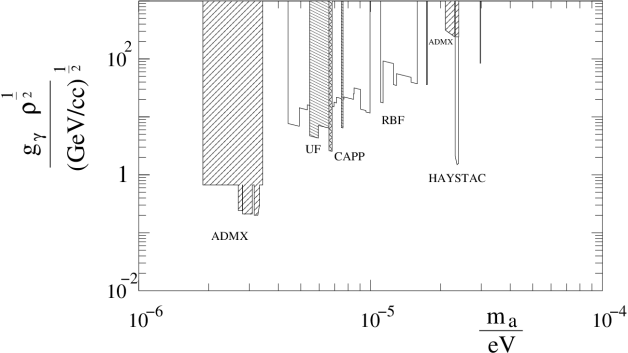
Figure 1: Limits on $g_{\gamma}\sqrt{\rho_{a}}$ where $g_{\gamma}$ is the dimensionless axion electromagnetic coupling, defined in Eq. (4), and $\rho_{a}$ is the local axion dark matter density, as a function of axion mass $m_{a}$, obtained by the RBF Wuensch et al. (1989), UF Hagmann (1990), ADMX Du et al. (2018); Boutan et al. (2018); Braine et al. (2020), HAYSTYAC Zhong et al. (2018) and CAPP-8TB Lee et al. (2020) cavity searches. Additional limits have been obtained by the ORGAN McAllister et al. (2017a) and QUAX_aγ Alesini et al. (2019a) experiments. The limits shown are in rough outline only.

Cavity searches for galactic halo axions have been carried out at Brookhaven National Laboratory De Panfilis et al. (1987); Wuensch et al. (1989), the University of Florida Hagmann et al. (1990a); Hagmann (1990), Kyoto University Matsuki and Yamamoto (1991); Tada et al. (1999), Lawrence Livermore National Laboratory Hagmann et al. (1998); Asztalos et al. (2001, 2002, 2004); Duffy et al. (2005, 2006); Asztalos et al. (2010), the University of Washington Asztalos et al. (2011); Hoskins et al. (2011, 2016); Du et al. (2018); Boutan et al. (2018); Braine et al. (2020), Yale University Brubaker et al. (2017b, a); Zhong et al. (2018), the Universty of Western Australia McAllister et al. (2017a), the INFN National Laboratory in Legnaro, Italy Alesini et al. (2019a) and the Center for Axion and Precision Physics (CAPP) in Daejeon, Korea Lee et al. (2020). New cavity detectors are under construction at CAPP Petrakou (2017); Semertzidis et al. (2019), and at CERN Álvarez Melcón et al. (2020). A large cavity detector is proposed at the INFN National Laboratory in Frascati Alesini et al. (2019b). A summary of limits from axion dark matter searches using the cavity technique is shown in Fig. 1.

IV.1 The signal

Axion to photon conversion occurs in large externally imposed electric $\vec{E}_{0}$ and/or magnetic $\vec{B}_{0}$ fields because the axion induced electric charge and current densities, Eqs. (24), are sources of electromagnetic waves. For non-relativistic axions, the

$$\vec{j}_{a}=-g~{}\vec{B}_{0}\partial_{t}a$$ (54)

term in the current density is most relevant since $\mid\partial_{t}a\mid>>\mid\vec{\nabla}a\mid$.

Consider an electromagnetic cavity, of volume $V$, inside of which exists a large static magnetic field $\vec{B}_{0}(\vec{x})$, dielectric constant $\epsilon(\vec{x})$ and magnetic permeability $\mu(\vec{x})$. We choose $\Phi=0$ gauge and expand the vector potential into cavity eigenmodes:

$$\vec{A}(\vec{x},t)=\sum_{\alpha}\vec{e}_{\alpha}(\vec{x})\psi_{\alpha}(t)~{}~{}~{}\ .$$ (55)

In the limit of vanishing skin depth, the normalized mode functions $\vec{e}_{\alpha}(\vec{x})$ satisfy:

$$\vec{\nabla}\cdot(\epsilon\vec{e}_{\alpha}) = 0$$

$$\vec{\nabla}\times({1\over\mu}\vec{\nabla}\times\vec{e}_{\alpha})-\epsilon\omega_{\alpha}^{2}\vec{e}_{\alpha} = 0$$

$$\hat{n}\times\vec{e}_{\alpha}\mid_{S} = 0$$

$$\int_{V}d^{3}x~{}\epsilon(\vec{x})~{}\vec{e}_{\alpha}(\vec{x})\cdot\vec{e}_{\beta}(\vec{x}) = \delta_{\alpha\beta}~{}~{}~{}\ ,$$ (56)

where $S$ is the surface of the cavity volume and $\hat{n}$ the unit normal to the surface. The $\omega_{\alpha}$ are the eigenfrequencies. In the absence of axions, the amplitudes $\psi_{\alpha}(t)$ satisfy

$$\Biggl{(}{d^{2}\over dt^{2}}+\gamma_{\alpha}{d\over dt}+\omega_{\alpha}^{2}\Biggr{)}\psi_{\alpha}(t)=0$$ (57)

where the term proportional to $\gamma_{\alpha}$ describes energy dissipation. $Q_{\alpha}={\omega_{\alpha}\over\gamma_{\alpha}}$ is the quality factor of the cavity in its $\alpha$-eigenmode.

We write the axion field as

$$a(\vec{x},t)=Re(A~{}e^{-i\omega_{a}t})~{}~{}~{}~{}\ .$$ (58)

Its $\vec{x}$-dependence is ignored because the cavity size is generally of order ${1\over m_{a}}$ whereas the de Broglie wavelength of halo axions is of order ${10^{3}\over m_{a}}$. Eq. (58) implies the local axion energy density:

$$\rho_{a}={1\over 2}\left((\partial_{t}a)^{2}+(\vec{\nabla}a)^{2}+m_{a}^{2}~{}a^{2}\right)={1\over 2}m_{a}^{2}|A|^{2}~{}~{}~{}~{}\ .$$ (59)

In the presence of axions, the $\psi_{\alpha}(t)$ satisfy the equation of motion

$$\Biggl{(}{d^{2}\over dt^{2}}+\gamma_{\alpha}{d\over dt}+\omega_{\alpha}^{2}\Biggr{)}\psi_{\alpha}(t)=-g~{}\int_{V}d^{3}x~{}\vec{B}_{0}(\vec{x})\cdot\vec{e}_{\alpha}(\vec{x})~{}Re(-i\omega_{a}Ae^{-i\omega_{a}t})~{}~{}~{}~{}\ ,$$ (60)

obtained by substituting Eqs. (55) and (58) into Eqs. (23), setting $\rho_{\rm el}=\vec{j}_{\rm el}=0$, and using Eqs. (56). The term describing energy dissipation was added by hand. Up to transients, the solution of Eq. (60) is

$$\psi_{\alpha}(t)=g~{}\omega_{a}~{}\Bigl{(}\int_{V}d^{3}x~{}\vec{B}_{0}\cdot\vec{e}_{\alpha}\Bigr{)}~{}Re\Bigl{(}{iA~{}e^{-i\omega_{a}t}\over\omega_{\alpha}^{2}-\omega_{a}^{2}-i\gamma_{\alpha}\omega_{a}}\Bigr{)}~{}~{}~{}~{}\ .$$ (61)

The time-averaged power from axion conversion into the $\alpha$-mode of the cavity is therefore

$$P_{\alpha} = \gamma_{\alpha}\int_{V}d^{3}x\left({1\over 2}\epsilon\vec{E}_{\alpha}\cdot\vec{E}_{\alpha}+{1\over 2\mu}\vec{B}_{\alpha}\cdot\vec{B}_{\alpha}\right)={\gamma_{\alpha}\over 2}[({d\psi_{\alpha}\over dt})^{2}+\omega_{\alpha}^{2}\psi_{\alpha}^{2}]$$ (62)

$$= {\gamma_{\alpha}\over 4}~{}{g^{2}\omega_{a}^{2}(\omega_{a}^{2}+\omega_{\alpha}^{2})\over(\omega_{\alpha}^{2}-\omega_{a}^{2})^{2}+\gamma_{\alpha}^{2}\omega_{a}^{2}}~{}|A|^{2}\left(\int_{V}d^{3}x\vec{B}_{0}(\vec{x})\cdot\vec{e}_{\alpha}(\vec{x})\right)^{2}~{}~{}~{}~{}\ .$$

The ratio of the energy of galactic halo axions to their energy spread is usually called the “quality factor” $Q_{a}$ of the axion signal. Eq. (52) indicates that $Q_{a}$ is of order $10^{6}$. If $Q_{a}>>Q_{\alpha}$ and the axion signal falls at the center of the cavity bandwidth ($\omega_{\alpha}=\omega_{a}$), Eq. (62) implies Sikivie (1983, 1985); Krauss et al. (1985)

$$P_{\alpha}=g^{2}\rho_{a}B_{0}^{2}VC_{\alpha}{1\over m_{a}}Q_{\alpha}$$ (63)

where $B_{0}$ is a nominal magnetic field inside the cavity and

$$C_{\alpha}\equiv{1\over B_{0}^{2}V}\Biggl{(}\int_{V}d^{3}x~{}\vec{B}_{0}(\vec{x})\cdot\vec{e}_{\alpha}(\vec{x})\Biggr{)}^{2}={\Biggl{(}\int_{V}d^{3}x\vec{B}_{0}(\vec{x})\cdot\vec{E}_{\alpha}(\vec{x})\Biggr{)}^{2}\over B_{0}^{2}V~{}\int_{V}d^{3}x~{}\epsilon(\vec{x})\vec{E}_{\alpha}(\vec{x})\cdot\vec{E}_{\alpha}(\vec{x})}~{}~{}~{}\ .$$ (64)

$C_{\alpha}$ expresses the coupling strength of mode $\alpha$ to galactic halo axions, and is called its “form factor”.

The conversion factor between mass and frequency is ($\hbar=c=1$)

$$10^{-5}~{}{\rm eV}=2\pi(2.418~{}{\rm GHz})~{}~{}~{}~{}~{}\ .$$ (65)

The GHz region is good hunting ground since $10^{-5}$ eV is a likely mass for axion dark matter. It is also convenient since an electromagnetic cavity whose fundamental mode has GHz frequency has size of order GHz^-1 = 30 cm. Expressed in practical units, Eq. (63) is

$$P_{\alpha} = 1.34\cdot 10^{-26}~{}{\rm Watt}\Biggl{(}{g_{\gamma}\over 0.36}\Biggr{)}^{2}\Biggl{(}{\rho_{a}\over{1\over 2}~{}10^{-24}~{}{\rm gr/cm^{3}}}\Biggr{)}\cdot$$ (66)

$$~{}~{}~{}~{}~{}~{}~{}~{}\cdot\Biggl{(}{B_{0}\over 8~{}{\rm Tesla}}\Biggr{)}^{2}\Biggl{(}{V\over{\rm m}^{3}}\Biggr{)}~{}C_{\alpha}~{}\Biggl{(}{m_{a}\over 2\pi~{}{\rm GHz}}\Biggr{)}Q_{\alpha}~{}\left({6\cdot 10^{15}~{}{\rm eV}^{2}\over f_{a}~{}m_{a}}\right)^{2}~{}~{}~{}\ .$$

The last factor in Eq. (66) is approximately one in view of Eq. (3). We include it here so that the numerical prefactor in Eq. (66) may be written with precision unmarred by the uncertainty in the relationship between $m_{a}$ and $f_{a}$.

Because the axion mass is unknown, the cavity should be tunable. In all experiments so far, tunability is achieved by inserting movable metal and/or dielectric posts inside the cavity. For the sake of definiteness, consider a cylindrical cavity in which exists a longitudinal homogeneous magnetic field $\vec{B}_{0}=B_{0}\hat{z}$  and a $z$-independent dielectric constant $\epsilon(x,y)$. By “cylindrical” cavity we mean one that is invariant under translations in the $\hat{z}$-direction, except for the endcaps Jackson (1998). The cross-sectional shape is arbitrary. Only the transverse magnetic (TM) modes of a cylindrical cavity couple to the axion field. Indeed the transverse electric (TE) and transverse electromagnetic (TEM) modes have vanishing form factor since their electric fields are perpendicular to $\vec{B}_{0}$. TM modes are labeled by three integers $\alpha=(l,n,p)$ with $\hat{z}\cdot\vec{e}_{lnp}\propto\cos{p\pi z\over L}$ and $p=0,1,2,...$, where $L$ is the length of the cavity. Only the TM_ln0 have non-zero form factor. For TM_ln0,

$$\vec{E}_{ln0}(\vec{x}) = \hat{z}~{}\phi_{ln}(x,y)$$ (67)

$$\Biggl{(}{\partial^{2}\over\partial x^{2}}+{\partial^{2}\over\partial y^{2}} + \epsilon(x,y)\omega_{ln0}^{2}\Biggr{)}\phi_{ln}=0$$ (68)

$$\phi_{ln}\mid_{S} = 0~{}~{}~{}~{}\ .$$ (69)

Here we assumed that the magnetic permeability $\mu=1$.

For a circular cross-section of radius R and $\epsilon=\mu=1$,

$$\phi_{ln}\propto J_{l}\left(x_{ln}{\rho\over R}\right)e^{il\theta}~{}~{},~{}~{}\omega_{ln0}={x_{ln}\over R}~{}~{},~{}~{}C_{ln0}={4\over(x_{on})^{2}}\delta_{l0}$$ (70)

where $(\rho,\theta)$ are axial coordinates and $x_{ln}$ is the $n^{th}$ zero of the Bessel function $J_{l}(x)$. In particular, $C_{010}=0.69$.

For a rectangular cross-section

$$\phi_{ln} \propto \sin\left({l\pi x\over L_{x}}\right)\sin\left({n\pi y\over L_{y}}\right)$$

$$C_{ln0} = {64\over\pi^{4}l^{2}n^{2}}~{}~{}~{}~{}~{}~{}~{}~{}~{}~{}~{}~{}{\rm for}~{}l~{}{\rm and}~{}n~{}{\rm odd}$$ (71)

$$= ~{}~{}0~{}~{}~{}~{}~{}~{}~{}~{}~{}~{}~{}~{}~{}~{}~{}~{}~{}{\rm otherwise}~{}~{}~{}~{}\ ,$$

where $L_{x}$ and $L_{y}$ are the transverse sizes.

Eqs. (70) and (71) show that, when $\vec{B}_{0}$ is homogeneous, the lowest TM mode has the strongest coupling. Indeed the electric field profiles $\phi_{ln}(x,y)$ of the higher TM modes have nodes, so that the contributions to the form factor from different regions of the cavity tend to cancel each other out.

IV.2 Signal to noise and search rate

The microwave power from axion conversion is coupled out through a small hole in the cavity walls and brought to the front end of a microwave receiver. The quality factor $Q$ of the cavity may be written

$${1\over Q}={1\over Q_{\rm h}}+{1\over Q_{\rm w}}~{}~{}~{}\ .$$ (72)

In Eq. (72) and henceforth we are suppressing the label $\alpha$ that indicates the mode dependence. $\gamma_{\rm h}={\omega\over Q_{\rm h}}$ is the contribution to $\gamma$ from emission through the hole and $\gamma_{\rm w}={\omega\over Q_{\rm w}}$ the contribution from absorption by the cavity walls. The maximum power that can be brought to the microwave receiver is $P_{\rm d}={Q\over Q_{\rm h}}P$ where $P$ is given by Eq. (66).

Because the cavity volume is permeated by a strong magnetic field, the cavity walls are ordinarily made of normal metal, although superconducting material can be used for the side walls van Bibber and Carosi (2013)Alesini et al. (2019a); Ahn et al. (2019). At low temperatures $(T\mathrel{\raise 1.29167pt\hbox{$<$\kern-10.50005pt\lower 4.30554pt\hbox{ $\sim$}}}$ few K) and frequencies $f$ in the GHz range, a cavity made of high purity copper has $Q_{\rm w}\sim 2\cdot 10^{5}$. In that case, the cavity bandwidth $B_{\rm c}\equiv f/Q$ is larger by a factor 10 or so than the bandwidth $B_{a}\equiv f/Q_{a}$ of the axion signal.

The axion signal is searched for by tuning the cavity to successive frequencies, separated by a cavity bandwidth $B_{\rm c}$ or less, and by integrating for an amount of time $t$ at each tune. To proceed at a reasonably fast rate, e.g. to cover a factor 2 in frequency in one year, the amount of time $t$ spent at each tune is of order ${1\over 3}{{\rm year}\over Q}\sim$ 100 seconds. ${1\over 3}$ is an assumed duty factor. During each time interval $t$, the power leaving the cavity is amplified by a receiver, shifted down in frequency by mixing with one or more local oscillators, digitized and spectrum analyzed. The signal can be analyzed with different resolutions. For example, the Axion Dark Matter Experiment (ADMX) Asztalos et al. (2001) has a 125 Hz medium resolution channel, hereafter called MedRes, obtained by co-adding many ($\sim 10^{4}$) short spectra taken during the measurement integration time $t$, and a high resolution channel, hereafter called HiRes, with 0.01 Hz resolution, the highest possible when $t=100$ sec. Any resolution less than $\delta f=1/t$ can be obtained by averaging the highest resolution spectrum.

When an axion signal is found, the energy spectrum of halo axions will immediately become known in great detail. So it is interesting to try and anticipate what that spectrum will look like.

As do all other cold effectively collisionless dark matter candidates, axions lie on a thin continuous 3-dimensional hypersurface in phase space. This hypersurface wraps and folds but does not break. This fact implies that, at any location and any time, dark matter axions form a discrete set of flows, each with a well defined density and velocity vector Sikivie and Ipser (1992); Natarajan and Sikivie (2005). Predictions for the velocity vectors and densities of the dark matter flows at our location in the Milky Way halo have been made Sikivie et al. (1995, 1997); Duffy and Sikivie (2008). Discrete flows are also produced when satellites, such as the Sagittarius dwarf galaxy Newberg et al. (2002); Majewski et al. (2003), are tidally disrupted by the gravitational field of the Milky Way. Discrete flows are called “streams” in this context. Each flow or stream at our location produces a narrow peak in the cavity detector, since the axions in the flow or stream have well defined kinetic energy in the laboratory frame. The peaks have a daily frequency modulation due to the Earth’s rotation and an annual frequency modulation due to the Earth’s orbital motion Ling et al. (2004). During 100 seconds of data taking, the frequency of a peak at 1 GHz shifts at most by $10^{-2}$ Hz due to the Earth’s rotation, and stays therefore within the $10^{-2}$ Hz highest possible resolution bandwidth. Because of each peak’s diurnal and annual modulations it is possible to measure the velocity vector of the associated flow or stream. Searching for narrow peaks increases the sensitivity of the cavity experiment provided a sufficiently large fraction of the local halo density is in one or more cold flows Duffy et al. (2005, 2006).

The output of the receiver chain is mostly noise, thermal noise from the cavity plus electronic noise from the receiver. If the axion signal frequency $\omega_{a}$ falls within the cavity bandwidth $B_{c}$, the output spectrum has extra power within the axion signal bandwidth $B_{a}$. The ratio $s\over n$ of the signal to a $1~{}\sigma$ fluctuation in the noise within a $B_{a}$ bandwidth is given by Dicke’s radiometer equation:

$${s\over n}={P_{\rm d}\over T_{\rm n}}\sqrt{{t\over B_{a}}}$$ (73)

where $T_{\rm n}$ is the total noise temperature. Each candidate peak is checked by taking more data. If the peak is a statistical fluctuation in the noise, it averages away. If a peak does not average away, it is a signal of something but most likely not an axion signal. The non-statistical peaks found so far have all been the result of leakage of microwave power into the cavity from the environment of the experiment. Such spurious signals are referred to as “environmental peaks”. It is straightforward to distinguish an axion signal from an environmental peak by exploiting the following properties: 1) an axion signal does not depend on the degree of microwave isolation of the cavity, 2) it cannot be picked up by a simple antenna outside the apparatus, 3) its dependence on the central frequency $\omega_{\alpha}$ of the cavity mode is a Lorentzian [see Eq. (62)], and 4) it is proportional to $B_{0}^{2}$.

In a search, every $p\sigma$ candidate peak is checked to see whether or not it is due to galactic halo axions. $p$ should be chosen neither too high nor too low. If too high, the search loses sensitivity. If too low, an excessive amount of time is wasted investigating fluctuations in the noise. In the ADMX MedRes channel, the noise is Gaussian-distributed because each spectrum is the sum of many independent spectra. There is therefore a 2.3% chance that the background fluctuates downward by $2\sigma$ or more in each $B_{a}$-wide bin. Hence, to put a 97.7% confidence level limit on the product $g_{\gamma}^{2}\rho_{a}$, the $s/n$ ratio must be $p+2$ and every candidate peak larger than $p\sigma$ ruled out as an axion signal. Through Eq. (73), this determines the minimum measurement integration time $t$ per cavity bandwidth $B_{\rm c}$ and hence the maximum rate at which the search may proceed in frequency space:

$${df\over dt}\simeq{B_{\rm c}\over t}={Q_{a}\over Q}{1\over(s/n)^{2}}\left({P_{\rm d}\over T_{\rm n}}\right)^{2}={1\over(s/n)^{2}}\left({P_{0}\over T_{n}}\right)^{2}Q_{a}{Q^{3}\over Q_{\rm h}^{2}}$$ (74)

where we used $P_{\rm d}={Q\over Q_{\rm h}}P$ and defined $P_{0}\equiv P/Q$. We may choose $Q_{\rm h}/Q_{\rm w}$ to maximize the search rate. One readily finds that the optimum occurs at $Q={1\over 3}Q_{\rm w}$, in which case

$${d\ln f\over dt} \simeq {1\over f}{1\over(s/n)^{2}}\left({P_{0}\over T_{n}}\right)^{2}Q_{a}\left({2\over 3}\right)^{2}Q$$ (75)

$$\simeq {27\over{\rm year}}\left({4\over s/n}\right)^{2}\left({V\over{\rm m}^{3}}\right)^{2}\left({B_{0}\over 8~{}{\rm T}}\right)^{4}C^{2}\cdot$$

$$\cdot \left({g_{\gamma}\over 0.36}\right)^{4}\left({\rho_{a}\over{1\over 2}~{}10^{-24}~{}{\rm gr/cm}^{3}}\right)^{2}\left({1~{}{\rm K}\over T_{\rm n}}\right)^{2}\left({f\over{\rm GHz}}\right)\left({Q\over{1\over 3}\cdot 10^{5}}\right)\left({Q_{a}\over 10^{6}}\right)\ ~{}~{}\ .$$

At GHz frequencies, electronic noise temperatures of order 2 K are achieved by using cooled Heterostructure Field-Effect Transistors (HFET) as microwave amplifiers Bradley (1999). The cavity is then cooled to liquid He temperatures so that the thermal noise qualitatively matches the electronic noise. This was the approach of the earliest experiments De Panfilis et al. (1987); Wuensch et al. (1989); Hagmann et al. (1990a). The experiment at Kyoto University Matsuki and Yamamoto (1991); Ogawa et al. (1996) explored the use of a beam of Rydberg atoms to detect the microwave photons from axion conversion. The more recent experiments Asztalos et al. (2010); Brubaker et al. (2017b) use Superconducting Quantum Interference Devices (SQUIDs) Muck et al. (1998, 2003) or Josephson Parametric Amplifiers (JPAs) Al Kenany et al. (2017). These devices approach the so-called ‘quantum limit’ defined by a noise temperature equal to the angular frequency in units where $k_{B}=\hbar=1$:

$$T_{n}=\omega=48~{}{\rm mK}\left({f\over{\rm GHz}}\right)~{}~{}\ .$$ (76)

To reduce thermal noise accordingly, the cavity is cooled to temperatures in the 100 mK range by a dilution refrigerator. The sensitivity of microwave photon detection for axion haloscopes may be boosted further by ‘vacuum squeezing’ Malnou et al. (2019) or single photon counting Lamoreaux et al. (2013); Kuzmin et al. (2018) techniques.

We may use Eq. (75) to estimate the search rate in the ADMX HiRes channel as well. When searching for peaks of width less than 0.01 Hz, the HiRes channel is sensitive to cold axion flows with quality factor $Q_{a}\mathrel{\raise 1.29167pt\hbox{$>$\kern-10.50005pt\lower 4.30554pt\hbox{ $\sim$}}}10^{11}$ at GHz frequencies. A large increase in $Q_{a}$ is the main motivation for the HiRes channel. However, it is partially offset by decreases in other parameters. The relevant $\rho_{a}$ is the density of the largest flow that produces a peak of width less than 0.01 Hz. If $\delta v$ is the velocity dispersion of a flow of cold axions, its energy dispersion is $\delta E\sim m_{a}v\delta v$ where $v\sim 10^{-3}$ is the flow velocity. Hence $Q_{a}>10^{11}$ requires $\delta v<$ 3 m/s. An additional consideration is that the noise is exponentially distributed in the HiRes channelDuffy et al. (2005, 2006) whereas it is Gaussian distributed in the MidRes channel. Because each HiRes spectrum has on the order of $Q_{c}/Q_{a}\sim 10^{6}$ bins, the threshold for a peak to be admitted as a candidate signal has to be set very high. The signal to noise ratio for a practical HiRes search was found to be of order 20 Duffy et al. (2005, 2006).

Ref. Chaudhuri et al. (2019) studies the sensitivity of a cavity haloscope that searches for a signal both inside and outside the cavity’s resonant bandwidth and optimizes the frequency-integrated sensitivity of such a search.

IV.3 Cavity design

After many years of improvement, the cavity technique has reached sufficient sensitivity to detect dark matter axions even with the weaker DFSZ value of the electromagnetic coupling Du et al. (2018); Boutan et al. (2018). The next challenge is to extend the technique to the widest possible axion mass range.

A large superconducting solenoid is the type of magnet that has been most commonly used for the experiment, although dipole, wiggler and toroidal magnets have specific advantages and are being considered as well Baker et al. (2012); Miceli (2015); Melcón et al. (2018). At first, the bore of a solenoidal magnet is filled with a single cylindrical cavity. Its resonant frequency may be tuned upwards approximately 50% by moving a metal post transversely from the side of the cavity to its center, and 30% downwards by similarly moving a dielectric rod Hagmann et al. (1990b). Provided longitudinal symmetry is maintained (the rods must extend from endcap to endcap and remain parallel to the cavity walls), the form factor $C$ stays of order one over the tuning range. If longitudinal symmetry is broken, the mode may become localized in a small part of the cavity. The form factor is then severely degraded.

To reach higher frequencies, one may fill up the volume available inside a magnet bore with many identical cavities and power-combine their outputs Hagmann et al. (1990b); Hagmann (1990). A two-port Wilkinson power combiner produces the output voltage ${1\over\sqrt{2}}(a+b~{}e^{-i\varphi})~{}e^{-i\omega t}$ when the input voltages are $a~{}e^{-i\omega t}$ and $b~{}e^{-i\varphi~{}-i\omega t}$. The power combiner adds the axion signals from the cavities provided that they are equal in magnitude and in phase. Thus one may power-combine the outputs of identical cavities provided that the largest distance between the cavities is less than the de Broglie wavelength ($\sim 10^{+3}/m_{a}$) of galactic halo axions, that the cavities are in tune, and that the phase-shifts between the individual cavities and the power combiner are identical. Since the noise in the different cavities is uncorrelated in phase, the noise temperature at the output of the power combiner is the average of the noise temperatures at its input ports. Properly built multi-cavity arrays have effective form factors of order one and allow, at the cost of engineering complexity, the upward extension of the frequency range over which a galactic halo axion search can be carried out with a given magnet.

Alternatively, one may reach higher frequencies by dividing a cavity into cells separated by metal vanes Stern et al. (2015); Jeong et al. (2018a, b). Such multi-cell cavities must be carefully designed to avoid mode crowding and mode localization. Ref. Kim et al. (2020) presents a design achieving a large form factor for the TM₀₃₀ mode of a cylindrical cavity by inserting dielectric vanes. Another proposal is to introduce materials that produce a plasma frequency for the electromagnetic field inside the cavity Lawson et al. (2019).

The frequency range of cavity haloscopes can also be extended upward by controlling the spatial variation of the magnetic field inside the cavity, or by introducing dielectric plates to control the mode structure. These two approaches are discussed in Section 5.1.

Refs. Sikivie (2010); Berlin et al. (2020); Lasenby (2020) propose to search for axion dark matter in an electromagnetic cavity which is driven with input power instead of being permeated by a magnetic field. The relevant process is $a+\gamma\rightarrow\gamma^{\prime}$ where $\gamma$ is a microwave photon in the mode that is driven by input power and $\gamma^{\prime}$ is a microwave photon, in another mode of the cavity, to be detected as signal. This approach can be pursued using an optical cavity as well Melissinos (2009).

Ref. Goryachev et al. (2019) proposes to search for dark matter axions by detecting the phase noise induced by the oscillating axion field in driven cavity modes separated in frequency by the axion mass. An experiment of this type is reported on in ref. Thomson et al. (2019).

V Other approaches to axion dark matter detection

The cavity technique works well for axion masses between perhaps $10^{-7}$ eV and a few times $10^{-5}$ eV but not, at any rate, for all masses that dark matter axions may plausibly have. So there is good motivation to look for alternatives. Over the years, different approaches have been proposed which collectively address the whole QCD axion mass range, from $10^{-2}$ eV to $10^{-12}$ eV. They are the topic of this Section. Several methods were anticipated in ref. Vorobev et al. (1995) and rediscovered later.

V.1 Wire arrays and dielectric plates

The conversion of axions to photons in a magnetic field can be enhanced by controlling the spatial variation of the magnetic field or by introducing dielectric plates to modify the mode structure of the electromagnetic field. In such schemes, it is likely useful to introduce a cavity as well.

V.1.1 Wire arrays

The differential cross-section for axion to photon conversion in a static magnetic field is given in Eq. (36). Multiplying by the axion flux $\beta_{a}n_{a}$ and integrating over solid angles yields the conversion rate

$$R={g^{2}n_{a}\over 16\pi^{2}\epsilon}\int d^{3}k~{}\delta({k\over\sqrt{\epsilon\mu}}-\omega)\sum_{\lambda=1,2}\bigg{|}\int_{V}d^{3}x~{}e^{i(\vec{k}_{a}-\vec{k})\cdot\vec{x}}~{}\hat{e}_{\lambda}(\hat{n})\cdot\vec{B}_{0}(\vec{x})\bigg{|}^{2}~{}~{}~{}\ .$$ (77)

To maximize $R$ for given field strength and volume, the magnetic field should be made inhomogeneous on the length scale set by the momentum transfer $\vec{q}=\vec{k}-\vec{k}_{a}$. Since dark matter axions are non-relativistic, $k_{a}<<k$ and hence $q\simeq k=\sqrt{\epsilon\mu}\omega\simeq\sqrt{\epsilon\mu}m_{a}$. So the inhomogeneity length scale should be of order ${1\over\sqrt{\epsilon\mu}m_{a}}$.

In view of this, it was proposed to build an array of superconducting wires embedded in a dielectric medium transparent to microwave radiation Sikivie et al. (1994). Magnetic fields are produced by passing electric currents through the wires. The dielectric medium keeps the wires in place. We set $\mu=1$ here for simplicity.

A possible realization consists of wires parallel to the $y$-axis whose intersections with the $xz$ plane form a regular lattice with lattice constant $d$. The wires intersect the $xz$ plane at $(n_{x}d,n_{z}d)$ where $n_{x}$ and $n_{z}$ are integers that range from $-{L_{x}\over 2d}$ to $+{L_{x}\over 2d}$, and $-{L_{z}\over 2d}$ and $+{L_{z}\over 2d}$ respectively. $L_{x}$ and $L_{z}$ are the dimensions of the detector in the $\hat{x}$ and $\hat{z}$ directions. The currents $I(n_{x},n_{z})$ in the wires are chosen to produce a particular magnetic field profile. For example

$$I(n_{x},n_{z})=I(n_{z})=I_{0}\sin(\kappa n_{z}d)$$ (78)

produces the magnetic field

$$\vec{B}=-\hat{x}{I_{0}\over\kappa d^{2}}\cos(\kappa z)$$ (79)

in the limit $L\rightarrow\infty$ and $d\rightarrow 0$. In practice the magnetic field deviates from Eq. (79) because of finite size $L$ and finite lattice constant $d$ effects. Such deviations, which can be calculated without much difficulty, are ignored here for simplicity.

For the sake of definiteness we assume Eq. (79) within a rectangular volume $V=L_{x}L_{y}L_{z}$. Because the photons produced are polarized in the direction $\hat{x}$, perpendicular to the wires, the effect of the wires on their propagation is minimized. In using Eq. (77) we are assuming that the photons propagate as if the wires were absent. For the magnitude squared of the space integral in Eq. (77) we have

$$\bigg{|}\int_{V}d^{3}x~{}e^{-i\vec{q}\cdot\vec{x}}B_{0}\cos(\kappa z)\bigg{|}^{2} = (2\pi)^{2}\delta_{L_{x}}(q_{x})\delta_{L_{y}}(q_{y})L_{x}L_{y}B_{0}^{2}\cdot$$ (80)

$$\cdot \left({\sin((q_{z}+\kappa)L_{z}/2)\over q_{z}+\kappa}+{\sin((q_{z}-\kappa)L_{z}/2)\over q_{z}-\kappa}\right)^{2}$$

where $\delta_{L}(q)$ is a Dirac delta-function spread over a width of order $1/L$. Resonant conversion is obtained for $q_{z}=\pm\kappa$. Since $\vec{k}\simeq\vec{q}$, the photons are emitted in the $\pm\hat{z}$ direction and can therefore be focused by mirrors onto one or two microwave receivers.

The wavevector $\kappa$ of the current configuration can be changed to tune the detector over a range of possible axion masses. The detector bandwidth is $\Delta k_{z}\simeq{\pi\over L_{z}}$ whereas the bandwidth of the axion signal is $\Delta k_{az}\simeq 2\cdot 10^{-3}m_{a}$. The conversion rate is obtained by inserting Eq. (80) into Eq. (77) and carrying out the integral over $\vec{k}$. Provided the axion signal falls entirely within the bandwidth of the detector, the signal power is

$$P = m_{a}R={g^{2}\over 8\sqrt{\epsilon}}VL_{z}B_{0}^{2}\rho_{a}$$ (81)

$$= 2\cdot 10^{-25}~{}{\rm W}\left({VL_{z}\over{\rm m}^{4}}\right)\left({B_{0}\over 8~{}{\rm T}}\right)^{2}\left({g_{\gamma}\over 0.36}\right)^{2}\left({m_{a}\over 10^{-5}~{}{\rm eV}}\right)^{2}{1\over\sqrt{\epsilon}}\left({\rho_{a}\over{1\over 2}\cdot 10^{-24}~{}{\rm g/cm}^{3}}\right)\ .$$

The discussion of the signal to noise and search rate is similar to that for the cavity detector in Section 4.2, and need not be repeated here.

The above design is convenient for signal calculation but not so convenient for construction and operation. In practice one wishes to minimize the number of connections between wires. A possible way to do this is to deform the above rectangular array into a cylinder so that all the wires at given $n_{z}$ combine to form a spiral. The spiral could be a NbTi strip etched by photolithographic techniques onto a low loss insulating sheet. The sheets would then be stacked to form the body of the detector.

Comparing Eqs. (63) and (81), the expression for the conversion power of a wire array is seen to be similar to that of a cavity haloscope but with the product $CQ$ of the cavity form and quality factors replaced by $L_{z}m_{a}/8\sqrt{\epsilon}$. If the axions have velocity dispersion $\delta v\sim 10^{-3}$, the requirement $\Delta k_{z}\mathrel{\raise 1.29167pt\hbox{$>$\kern-10.50005pt\lower 4.30554pt\hbox{ $\sim$}}}\Delta k_{a}$ implies $L_{z}m_{a}\mathrel{\raise 1.29167pt\hbox{$<$\kern-10.50005pt\lower 4.30554pt\hbox{ $\sim$}}}1,600$. When searching for low velocity dispersion flows, such as the Big Flow of Eq. (19), $L_{z}m_{a}$ can be made much larger. However the detector must in that case be kept aligned with respect to a particular flow.

It is generally advantageous to place the wire array inside an electromagnetic cavity Rybka et al. (2015). A small wire array was built at the University of Washington and placed in an open Fabry-Perot resonator, in an experiment called ORPHEUS Rybka et al. (2015). A schematic drawing of such a setup is shown in Fig. 2. The detector is now in effect a cavity haloscope and the considerations of Section 4 apply to it. If the electric field for the Fabry-Perot mode is

$$\vec{E}_{\omega}=\hat{x}E_{\omega}\cos(\kappa z)$$ (82)

within the volume of the wire array, and the magnetic field is as in Eq. (79), the conversion power is given by Eq. (63) with $V$ being the volume of the wire array and $C=0.5~{}F$, where $F$ is the fraction of the distance between the mirrors that is occupied by the wire array. The detector is tuned by changing the distance between the mirrors. In the ORPHEUS detector, the distances between the wire planes were changed proportionately.

V.1.2 Dielectric plates

Instead of making the magnetic field inhomogeneous on the $q^{-1}\sim m_{a}^{-1}$ length scale, one may instead have the dielectric constant vary on that length scale Morris (1984); Caldwell et al. (2017); McAllister et al. (2018); Ioannisian et al. (2017); Millar et al. (2017); Baryakhtar et al. (2018). MADMAX Brun et al. (2019) is a proposed experiment using dielectric plates, although in a different manner from the setup described below. MADMAX evolved from an earlier broadband axion dark matter detection scheme, called the dish antenna Horns et al. (2013).

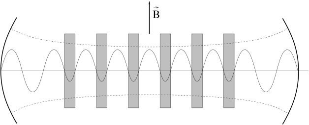
Figure 3: Dielectric plate detector of dark matter axions discussed in Section 5.1.2. The dashed lines represent the envelope of an electromagnetic mode in a confocal resonator. The mode is driven by axion to photon conversion in a uniform static externally applied magnetic field $\vec{B}$. The vertical shaded rectangles represent dielectric plates arranged in such a way as to make the overlap integral of the applied static magnetic field $\vec{B}$ with the oscillating electric field of the mode as large as possible. The electric field profile of the mode is shown.

Here we consider a stack of parallel plates of thickness $d$ and dielectric constant $\epsilon$ placed in a Fabry-Perot resonator, as shown schematically in Fig. 3. The distance $D$ between the plates is chosen to be the half-wavelength ${\pi\over m_{a}}$ in vacuum of the photons produced by axion conversion, whereas the plate thickness $d$ is chosen to be of order the half-wavelength ${\pi\over\sqrt{\epsilon}m_{a}}$ of those photons in the dielectric material. The intended electric field profile of the electromagnetic mode in the region occupied by the dielectric plates is

$$\vec{E}_{\omega} = \hat{x}E_{\omega}\sin(\omega(z-z_{j}))~{}~{}~{}~{}~{}~{}~{}~{}~{}~{}{\rm for}~{}~{}0\leq z-z_{j}\leq D$$ (83)

$$= \hat{x}{E_{\omega}\over\sqrt{\epsilon}}\sin(\sqrt{\epsilon}\omega(z-z_{j}))~{}~{}~{}~{}~{}~{}{\rm for}-d\leq z-z_{j}\leq 0$$

where the $z_{j}$ are the positions of the right faces of the plates; see Fig. 3. With this electric field profile and a unifrom magnetic field $\vec{B}_{0}=B_{0}\hat{x}$, the conversion power is given by Eq. (63) with $V$ being the volume of the stack of plates (including the spaces between plates) and

$$C={8\over\pi^{2}}~{}{(\epsilon-1)^{2}\over\epsilon(\sqrt{\epsilon}+1)^{2}}~{}F~{}\ ,$$ (84)

where $F$ is the fraction of the distance between the mirrors that is occupied by the stack of plates. Some materials (e.g. Al₂O₃) have high dielectric constant ($\epsilon\sim 10$) but low dielectric losses ($\tan\delta_{e}\sim 10^{-4}$). The mirrors, if placed outside the magnetic field region, can be made of superconducting material so that their contribution to dissipative losses is small.

V.2 Magnetic resonance

Ignoring the small CP violating term shown explicitly in Eq. (9), the interaction energy of the axion with a non-relativistic electron is

$$H_{a\bar{e}e}={g_{e}\over 2f_{a}}(\vec{\nabla}a\cdot\vec{\sigma}+\partial_{t}a~{}{\vec{p}\cdot\vec{\sigma}\over m_{e}})$$ (85)

where $\vec{p}$ is the electron momentum, $m_{e}$ its mass and $\vec{S}={1\over 2}\vec{\sigma}$ its spin. The first term in Eq. (85) is similar to the coupling of a magnetic field to electron spin. The effective magnetic field associated with a gradient in the axion field is

$$\vec{B}_{\rm eff}=-{g_{e}\over\gamma_{e}f_{a}}\vec{\nabla}a$$ (86)

where $\gamma_{e}$ is the electron gyromagnetic ratio. The axion has analogous interactions (9) with quarks. We therefore expect an interaction energy of the axion field with nuclear spin $\vec{I}$

$$H_{a\bar{N}N}={g_{N}\over f_{a}}\vec{\nabla}a\cdot\vec{I}$$ (87)

where the $g_{N}$ are dimensionless couplings of order one that are determined by nuclear physics in terms of $g_{p}$ and $g_{n}$  Stadnik and Flambaum (2015). Eqs. (85) and (87) suggest that one may search for dark matter axions using magnetic resonance techniques. Refs. Barbieri et al. (1989, 2017) proposed to detect the power from axion to magnon conversion in a medium containing a high density of aligned electron spins. Refs. Graham and Rajendran (2013); Budker et al. (2014) proposed to detect the transverse magnetization induced by the axion field onto a sample of aligned nuclear spins.

Let us briefly recall basic aspects of magnetic resonance Kittel (1968). A macroscopic sample of particles with spin $\vec{I}$ and magnetic moment

$$\vec{\mu}=\gamma\vec{I}$$ (88)

is polarized in a static magnetic field $\vec{B_{0}}=B_{0}\hat{z}$, or by some other means, resulting in a magnetization $M_{0}\hat{z}$. We use $\vec{I}$ to represent electron spin ${1\over 2}\vec{\sigma}$ or nuclear spin, whichever applies. In addition to $\vec{B}_{0}$, a weak transverse time-dependent magnetic field $\vec{B}_{\perp}=\hat{x}B_{x}(t)+\hat{y}B_{y}(t)$ is applied. The transverse components of the magnetization satisfy the Bloch equations

$${dM_{x}\over dt} = \gamma(\vec{M}\times\vec{B})_{x}-{1\over t_{2}}M_{x}=-\gamma M_{0}B_{y}+\gamma B_{0}M_{y}-{1\over t_{2}}M_{x}$$

$${dM_{y}\over dt} = \gamma(\vec{M}\times\vec{B})_{y}-{1\over t_{2}}M_{y}=+\gamma M_{0}B_{x}-\gamma B_{0}M_{x}-{1\over t_{2}}M_{y}$$ (89)

where $t_{2}$ is the transverse relaxation time. When $\vec{B}_{\perp}=0$, an initial transverse magnetization precesses about the $z$-axis with angular frequency $\omega_{0}=-\gamma B_{0}$ and decays in a time $t_{2}$. For the sake of definiteness, we assume that the $\hat{z}$-axis is chosen so that $\omega_{0}>0$. If the transverse field has the form

$$\vec{B}_{\perp}(t)=B_{\perp}(\hat{x}\cos\omega t+\hat{y}\sin\omega t)~{}~{}\ ,$$ (90)

the sample acquires in steady state the transverse magnetization

$$\vec{M}_{\perp}=M_{\perp}[\hat{x}\cos(\omega t-\phi)+\hat{y}\sin(\omega t-\phi)]$$ (91)

with

$$\tan\phi={1\over(\omega_{0}-\omega)t_{2}}$$ (92)

and

$$M_{\perp}={\gamma M_{0}t_{2}B_{\perp}\over\sqrt{1+(\omega_{0}-\omega)^{2}t_{2}^{2}}}~{}~{}\ .$$ (93)

On resonance ($\omega=\omega_{0}$) the transverse magnetization has its maximum magnitude $\gamma M_{0}t_{2}B_{\perp}$ and its phase is $\pi/2$ behind that of $\vec{B}_{\perp}$.

We now consider a magnetized sample bathed in a flow of axions described by the field

$$a(\vec{x},t)=A\sin(\vec{k}\cdot\vec{x}-\omega t)~{}~{}~{}\ ,$$ (94)

with $\omega=\sqrt{m_{a}^{2}+\vec{k}\cdot\vec{k}}\simeq m_{a}+{k^{2}\over 2m_{a}}$. The energy density of such a flow is

$$\rho_{a}={1\over 2}\omega^{2}A^{2}~{}~{}\ .$$ (95)

Comparing (87) with the interaction $H_{B}=-\gamma\vec{I}\cdot\vec{B}$ of a magnetic field with spin, the axion field (94) is seen to produce an effective tranverse magnetic field

$$\vec{B}_{\perp,{\rm eff}}=-{1\over\gamma}{g_{N}\over f_{a}}A\vec{k}_{\perp}\cos(\omega t)$$ (96)

where $\vec{k}_{\perp}=\vec{k}-\hat{z}(\hat{z}\cdot\vec{k})$. In contrast to Eq. (90), it drives the transverse magnetization in only one spatial direction. Also, the field due to dark matter axions in the Milky Way halo does not have the infinite coherence time implied by Eq. (90) or (94). The direction and time-dependence of $\vec{B}_{\perp,{\rm eff}}$ depends on the model of the galactic halo. Two contrasting proposals were mentioned in Section 2. In the isothermal model, the energy dispersion $\delta\omega\simeq 10^{-6}m_{a}$, and hence the coherence time $t_{c}=1/\delta\omega\simeq 0.16~{}{\rm sec}({\rm MHz}/\nu_{a})$ where $\nu_{a}$ is the frequency associated with the axion mass: $m_{a}=2\pi\nu_{a}$. In the caustic ring model, the local dark matter density is dominated by a single flow, the Big Flow, with velocity dispersion $\delta v\mathrel{\raise 1.29167pt\hbox{$<$\kern-10.50005pt\lower 4.30554pt\hbox{ $\sim$}}}$ 70 m/s. Its energy dispersion $\delta\omega=m_{a}v\delta v\mathrel{\raise 1.29167pt\hbox{$<$\kern-10.50005pt\lower 4.30554pt\hbox{ $\sim$}}}2\cdot 10^{-10}m_{a}$ and hence its coherence time $t_{c}\mathrel{\raise 1.29167pt\hbox{$>$\kern-10.50005pt\lower 4.30554pt\hbox{ $\sim$}}}700$ sec (MHz/$\nu_{a}$).

V.2.1 Nuclear magnetic resonance (NMR)

When the transverse magnetic field is in only one spatial direction, say $\vec{B}_{\perp}(t)=B_{\perp}\cos(\omega t)\hat{x}$, the Bloch equations are solved by

$$\vec{M}_{a}(t)=M_{\perp a}[\hat{x}\cos(\omega t-\phi)+\hat{y}\sin(\omega t-\phi)]+{\cal O}({1\over\omega+\omega_{0}})$$ (97)

with $\phi$ given in Eqs. (92) and

$$M_{\perp a}={1\over 2}{\gamma M_{0}t_{2}B_{\perp}\over\sqrt{1+(\omega_{0}-\omega)^{2}t_{2}^{2}}}~{}~{}\ .$$ (98)

The terms of order $(\omega+\omega_{0})^{-1}$ in Eq. (97) are nonresonant and can be ignored. The effect of frequency dispersion in the axion field is included by replacing $t_{2}$ with $\min(t_{2},t_{c})$. We have then on resonance $(\omega_{0}=m_{a})$

$$M_{\perp a} = {g_{N}\over f_{a}}v_{\perp}\sqrt{\rho_{a}\over 2}M_{0}\min(t_{2},t_{c})$$ (99)

$$= 0.5\cdot 10^{-14}~{}M_{0}~{}g_{N}\left({m_{a}\over 10^{-8}~{}{\rm eV}}\right)\left({v_{\perp}\over 10^{-3}}\right)\left({\rho_{a}\over{\rm GeV/cm}^{3}}\right)^{1\over 2}{\min(t_{2},t_{c})\over{\rm sec}}~{}~{}\ .$$

The transverse magnetization may be detected by a SQUID magnetometer. The present sensitivity of such devices is of order $10^{-16}~{}{\rm T}/\sqrt{\rm Hz}$. The CASPEr-Wind experiment Budker et al. (2014); Garcon et al. (2017) searches for axion dark matter using this technique.

Refs. Graham and Rajendran (2013); Budker et al. (2014); Garcon et al. (2017) propose a second approach to axion dark matter detection using NMR techniques, called CASPEr-Electric. In it a static electric field $\vec{E}_{0}$ is applied in a direction transverse to $\vec{M}_{0}$. The electric field interacts with the oscillating electric dipole moment induced onto the nucleus by the local axion field

$$\vec{d}_{e}(t)=D_{N}\bar{\theta}(t)\vec{I}=D_{N}{a(t)\over f_{a}}\vec{I}$$ (100)

where $D_{N}\sim 3\cdot 10^{-16}~{}e$ cm; see Eq. (2). The relevant interaction is thus

$$H_{a\bar{N}N}^{\prime}=-\vec{d}_{e}\cdot\vec{E}_{N}=-D_{N}{a(t)\over f_{a}}\vec{I}\cdot\vec{E}_{N}$$ (101)

where $\vec{E}_{N}$ is the electric field at the location of the nucleus. In an atom, a static externally applied electric field $\vec{E}_{0}$ is screened at the location of the nucleus by the electron cloud, implying $\vec{E}_{N}=0$. Indeed, if $\vec{E}_{N}\neq 0$, the nucleus moves till $\vec{E}_{N}=0$. However, because of finite nuclear size effects, $\vec{E}_{N}$ does not vanish entirely but is suppressed by a factor $\epsilon_{S}$, called the Schiff factor, of order $10^{-2}$ for a large nucleus Graham and Rajendran (2013); Budker et al. (2014). Relative to $H_{a\bar{N}N}$ the strength of the interaction $H_{a\bar{N}N}^{\prime}$ is then

$${\epsilon_{S}D_{N}E_{0}\over g_{N}v_{\perp}m_{a}}\sim 10^{4}~{}\left({\epsilon_{s}\over 10^{-2}}\right)\left({E_{0}\over 3\cdot 10^{8}~{}{\rm V/cm}}\right)\left({10^{-10}~{}{\rm eV}\over m_{a}}\right)$$ (102)

suggesting that this approach is attractive for small axion masses.

V.2.2 Axion to magnon conversion

When the axion field excites transverse magnetization, axions are converted to magnons Barbieri et al. (1989, 2017); Chigusa et al. (2020). Whereas an amplitude measurement, such as CASPEr is more sensitive at low frequencies, a power measurement is more sensitive at hign frequencies. The power from axion to magnon conversion on resonance ($\omega_{0}=m_{a}$) is

$$P_{m} = -\vec{M}_{\perp a}\cdot{d\vec{B}_{\perp,{\rm eff}}\over dt}V=m_{a}M_{\perp a}B_{\perp,{\rm eff}}V$$ (103)

$$= \left({g_{e}\over f_{a}}\right)^{2}m_{a}\rho_{a}(v_{\perp})^{2}{M_{0}V\over\gamma}\min(t_{2},t_{c})$$

$$= 7.9\cdot 10^{-20}~{}{\rm W}~{}g_{e}^{2}\left({m_{a}\over 10^{-4}~{}{\rm eV}}\right)^{3}\left({n_{s}V\over 10^{24}}\right)\left({v_{\perp}\over 10^{-3}}\right)^{2}\left({\rho_{a}\over{\rm GeV/cm}^{3}}\right){\min(t_{2},t_{c})\over{\rm sec}}$$

in a volume $V$ of aligned electron spins with density $n_{s}$. The QUAX experiment at the INFN Laboratory in Legnaro, Italy, searches for axion dark matter using a magnetized sample placed in an electromagnetic cavity Barbieri et al. (2017); Crescini et al. (2018, 2020). The electron spins are coupled to a cavity resonant mode, tuned to the frequency $\omega_{0}$, so that the magnons convert to microwave photons. The electromagnetic power is coupled out and detected by a microwave receiver. The cavity is cooled to temperatures of order 100 mK to suppress thermal noise. The approach is discussed also in Flower et al. (2019) with results from an initial experiment.

V.3 LC circuit

For axion masses below $10^{-7}$ eV, the size of the cavity detector is of order 10 m or larger. For such small masses it may be advantageous to replace the cavity by a LC circuit Sikivie et al. (2014); Kahn et al. (2016); McAllister et al. (2016); Silva-Feaver et al. (2017); Chu et al. (2018); Crisosto et al. (2018); Chaudhuri et al. (2018); Ouellet et al. (2019b, a); Crisosto et al. (2020) .

Eqs. (23) tell us that in an externally applied magnetic field $\vec{B}_{0}$ dark matter axions produce an electric current density $\vec{j}_{a}=-g\vec{B}_{0}\partial_{t}a$. Assuming the magnetic field is static, $\vec{j}_{a}$ oscillates with frequency $\omega=m_{a}(1+{1\over 2}\vec{v}\cdot\vec{v})$ where $\vec{v}$ is the axion velocity. If the spatial extent of the externally applied magnetic field is much less than $\omega^{-1}$, the Maxwell displacement current $\partial_{t}(\epsilon\vec{E})$ can be neglected in the second equation (23). The magnetic field $\vec{B}_{a}$ produced by $\vec{j}_{a}$ satisfies then $\vec{\nabla}\times\vec{B}_{a}=\vec{j}_{a}$. We set $\mu=1$ for simplicity. One may amplify $\vec{B}_{a}$ using an LC circuit and detect the amplified field with a SQUID magnetometer.

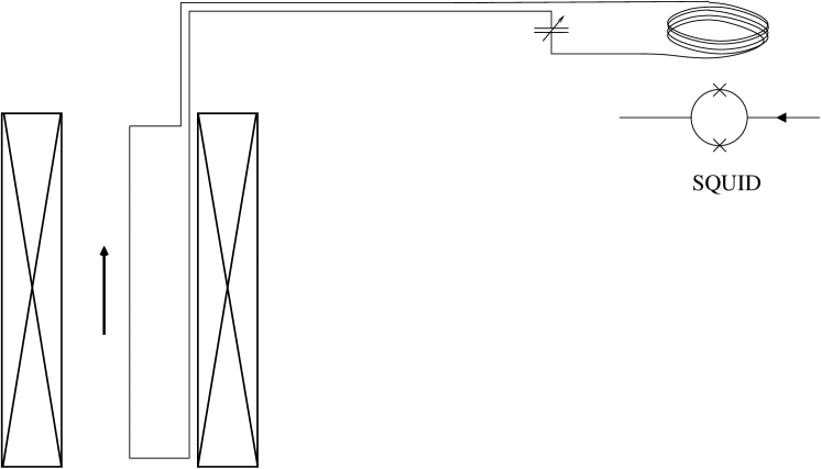
Figure 4: Schematic drawing of the LC circuit axion dark matter detector in case the magnet is a solenoid. The two crossed rectangles indicate cross-sections of the solenoid’s windings. The arrow shows the direction of the magnetic field that the solenoid produces. This figure is reproduced from ref. Sikivie et al. (2014).

Fig. 4 shows a schematic drawing in case the magnet producing $\vec{B}_{0}$ is a solenoid. The field $\vec{B}_{a}$ has flux $\Phi_{a}$ through a loop of superconducting wire. Because the wire is superconducting the total magnetic flux through the loop circuit is constant. In the limit where the capacitance $C$ of the circuit is infinite (the capacitance is removed) the current in the wire is $I=-\Phi_{a}/L$ where $L$ is the inductance of the circuit. The magnetic field seen by the magnetometer is

$$B_{d}\simeq{N_{d}\over 2r_{d}}I=-{N_{d}\over 2r_{d}~{}L}\Phi_{a}$$ (104)

where $N_{d}$ is the number of turns and $r_{d}$ the radius of the small coil facing the magnetometer. Ignoring for the moment the mutual inductances of the LC circuit with neighboring circuits in its environment, $L$ is a sum

$$L\simeq L_{m}+L_{c}+L_{d}$$ (105)

of contributions $L_{m}$ from the large pickup loop inside the externally applied magnetic field, $L_{d}$ from the small coil facing the magnetometer, and $L_{c}$ from the co-axial cable in between. We have

$$L_{d}=r_{d}N_{d}^{2}c_{d}$$ (106)

with

$$c_{d}\simeq\ln\left({8r_{d}\over a_{d}}\right)-2$$ (107)

where $a_{d}$ is the radius of the wire in the small coil. The mutual inductances of the LC circuit with neighboring circuits can be measured in any actual setup and taken into account when optimizing the circuit and estimating the detector’s sensitivity.

For finite $C$, the LC circuit resonates at frequency $\omega=1/\sqrt{LC}$. When $\omega$ equals the axion rest mass, the magnitude of the current in the wire is multiplied by the quality factor $Q$ of the circuit and hence

$$B_{d}\simeq{QN_{d}\Phi_{a}\over 2Lr_{d}}~{}~{}~{}\ .$$ (108)

Let us consider the case where the externally applied magnetic field is homogeneous, $\vec{B}_{0}=B_{0}\hat{z}$, as is approximately true inside a long solenoid. In such a region

$$\vec{B}_{a}=-{1\over 2}g(\partial_{t}a)B_{0}\rho\hat{\phi}$$ (109)

where ($z$, $\rho$, $\phi$) are cylindrical coordinates. For the pickup loop depicted in Fig. 4, a rectangle whose sides $l_{m}$ and $r_{m}$ are approximately the length and radius of the magnet bore, the flux of $\vec{B}_{a}$ through the pickup loop is

$$\Phi_{a}=-V_{m}gB_{0}\partial_{t}a$$ (110)

with $V_{m}={1\over 4}l_{m}r_{m}^{2}$. Assuming $l_{m}>>r_{m}$, the self-inductance of the pickup loop is $L_{m}\simeq{1\over\pi}l_{m}\ln\left({r_{m}\over a_{m}}\right)$ where $a_{m}$ is the radius of the wire.

The time derivative of the axion field is given in terms of the axion density by $\partial_{t}a=\sqrt{2\rho_{a}}\cos(\omega t)$. Hence, combining Eqs. (108) and (110), we obtain the magnitude of the magnetic field seen by the magnetometer:

$$B_{d} \simeq {N_{d}Q\over 2r_{d}L}V_{m}g\sqrt{2\rho_{a}}B_{0}=1.25\cdot 10^{-15}~{}{\rm T}\left({\rho_{a}\over{\rm GeV/cm}^{3}}\right)^{1\over 2}\left({Q\over 10^{4}}\right)\cdot$$ (111)

$$\cdot \left({g\over 10^{-17}~{}{\rm GeV}^{-1}}\right)N_{d}\left({{\rm cm}\over r_{d}}\right)\left({V_{m}\over{\rm m}^{3}}\right)\left({\mu{\rm H}\over L}\right)\left({B_{0}\over 10~{}{\rm T}}\right)\ .$$

In comparison, the sensitivity of today’s best magnetometers is $\delta B=B_{n}\sqrt{\Delta\nu\over{\rm Hz}}$ with $B_{n}$ of order $10^{-16}~{}{\rm T}$. The detector bandwidth is $\nu/Q$. If a factor 2 in frequency is to be covered per year, and the duty factor is 30%, the amount of time $t$ spent at each tune of the LC circuit is of order $10^{7}~{}{\rm s}/Q$. The signal to noise ratio depends on the signal coherence time $t_{c}$ and hence on the axion velocity distribution. The coherence times of two contrasting galactic halo models were given in the previous subsection. The magnetometer is sensitive to magnetic fields of magnitude $\delta B=B_{n}~{}({\rm t~{}Hz})^{-{1\over 2}}$ when $t<t_{c}$ and $\delta B=B_{n}~{}({\rm Hz})^{-{1\over 2}}~{}(t_{c}~{}t)^{-{1\over 4}}$ when $t>t_{c}$.

An important source of noise, in addition to the flux noise in the magnetometer, is the thermal (Johnson-Nyquist) noise in the LC circuit. It causes voltage fluctuations $~{}\delta V_{T}=\sqrt{4k_{B}T~{}R~{}\Delta\nu}~{}$ Nyquist (1928) and hence current fluctuations

$$\delta I_{T} = {\delta V_{T}\over R}=\sqrt{4k_{B}TQ\Delta\nu\over L\omega}$$ (112)

$$= 2.96\cdot 10^{-13}{\rm A}\sqrt{\left({{\rm MHz}\over\nu}\right)\left({\mu{\rm H}\over L}\right)\left({Q\over 10^{4}}\right)\left({T\over{\rm mK}}\right)\left({\Delta\nu\over{\rm mHz}}\right)}$$

where we used the relation $R={L\omega\over Q}$ between the resistance and quality factor of a LC circuit. Eq. (112) should be compared with the current due to the signal

$$I = {Q\over L}V_{m}gB_{0}\partial_{t}a=1.99\cdot 10^{-11}{\rm A}\left({Q\over 10^{4}}\right)\left({V_{m}\over{\rm m}^{3}}\right)\left({\mu{\rm H}\over L}\right)\cdot$$ (113)

$$\cdot \left({g\over 10^{-17}{\rm GeV}^{-1}}\right)\sqrt{\rho_{a}\over{\rm GeV}/{\rm cm}^{3}}\left({B_{0}\over 10~{}{\rm T}}\right)$$

and with the fluctuations in the measured current due to the noise in the magnetometer

$$\delta I_{B}\simeq{2r_{d}\over N_{d}}\delta B=5.03\cdot 10^{-14}{\rm A}{1\over N_{d}}\left({r_{d}\over{\rm cm}}\right)\left({B_{n}\over 10^{-16}~{}{\rm T}}\right)\sqrt{\Delta\nu\over{\rm mHz}}\ .$$ (114)

Another possible source of noise is jumps in the $\vec{B}_{0}$ field, caused by small sudden displacements in the positions of the wires in the magnet windings.

The LC circuit detector appears well suited to axion dark matter detection in the $10^{-7}$ to $10^{-9}$ eV range. The ABRACADABRA experiment at MIT Kahn et al. (2016); Ouellet et al. (2019b, a) and ADMX SLIC experiment at the University of Florida Crisosto et al. (2018, 2020) have published results. An experiment is also under construction at Stanford (DM Radio) Silva-Feaver et al. (2017); Chaudhuri et al. (2018).

A reentrant cavity is an electromagnetic cavity with properties similar to those of an LC circuit. Ref. McAllister et al. (2017b) describes such a cavity and computes its form factor as a function of frequency.

V.4 Atomic transitions

The interaction of an axion with a non-relativistic electron, Eq. (85) and the interaction of an axion with nuclear spin, Eq. (87), allow atomic transitions in which an axion is emitted or absorbed. The transitions are resonant between atomic states that differ in energy by an amount equal to the axion mass. Such energy differences can be conveniently tuned using the Zeeman and Stark effects. One approach to axion dark matter detection is to cool a kilogram-sized sample to milli-Kelvin temperatures and count axion induced atomic or molecular transitions using laser techniques Sikivie (2014); Santamaria et al. (2015); Braggio et al. (2017); Avignone et al. (2018a).

Eq. (87) and the first term on the RHS of Eq. (85) are similar to the coupling of the magnetic field to spin. Those interactions may cause magnetic dipole (M1) transitions in atoms and molecules. The second term in Eq. (85) allows $\Delta j=0$, $\Delta l=1$, parity changing transitions. As usual, $l$ is the quantum number giving the magnitude of orbital angular momentum, and $j$ that of total angular momentum. We will not consider that last interaction further because, starting from the ground state ($l=0$), it causes atomic transitions only if the energy absorbed is of order eV, much larger than the axion mass. Molecular transitions in the eV range are discussed as a technique for dark matter detection in ref. Arvanitaki et al. (2018).

The ground state of most atoms is accompanied by several other states related to it by hyperfine splitting, i.e. by flipping the spin of one or more valence electrons or by changing the $z$-component $I_{z}$ of the nuclear spin. The transition rate by axion absorption from an atomic ground state $|0\rangle$ to an excited state $|i\rangle$ is

$$R_{i}={1\over 2m_{a}f_{a}^{2}}\min(t,t_{1},t_{c})~{}\int d^{3}p~{}~{}{d^{3}n\over dp^{3}}(\vec{p})~{}|\langle i|(g_{e}\vec{S}+g_{N}\vec{I})\cdot\vec{p}|0\rangle|^{2}$$ (115)

on resonance. Here $\vec{S}$ is electron spin, $t$ is the measurement integration time, $t_{1}$ the lifetime of the excited state, and $t_{c}$ the coherence time of the signal. The latter is related to the energy dispersion of dark matter axions, $t_{c}\sim 1/\delta E$, as was discussed already. The resonance condition is $m_{a}=E_{i}-E_{0}$ where $E_{i}$ and $E_{0}$ are the energies of the two states. The detector bandwidth is $B=1/\min(t,t_{1})$. ${d^{3}n\over dp^{3}}(\vec{p})$ is the local axion momentum distribution. The local axion energy density is

$$\rho_{a}\simeq m_{a}\int d^{3}p~{}{d^{3}n\over dp^{3}}(\vec{p})~{}~{}\ .$$ (116)

Let us define $g_{i}$ by

$$g_{i}^{2}\overline{v^{2}}m_{a}\rho_{a}\equiv\int d^{3}p~{}{d^{3}n\over dp^{3}}(\vec{p})~{}|\langle i|(g_{e}\vec{S}+g_{N}\vec{I})\cdot\vec{p}|0\rangle|^{2}~{}~{}\ ,$$ (117)

where $\overline{v^{2}}\sim 10^{-6}$ is the average velocity squared of dark matter axions. $g_{i}$ is a number of order one giving the coupling strength of the target atom. $g_{i}$ depends on the atomic transition used, the direction of polarization of the atom, and the momentum distribution of the axions. It varies with time of day and of year since the momentum distribution changes on those time scales due to the motion of the Earth.

For a mole of target atoms, the transition rate on resonance is

$$N_{A}R_{i} = g_{i}^{2}N_{A}~{}\overline{v^{2}}~{}{\rho_{a}\over 2f_{a}^{2}}\min(t,t_{1},t_{c})$$ (118)

$$= ~{}{535\over{\rm sec}}\left({\rho_{a}\over{\rm GeV}/{\rm cm}^{3}}\right)\left({10^{11}~{}{\rm GeV}\over f_{a}}\right)^{2}g_{i}^{2}~{}\left({\overline{v^{2}}\over 10^{-6}}\right){\min(t,t_{1},t_{c})\over{\rm sec}}$$

where $N_{A}$ is Avogadro’s number. There is an (almost) equal transition rate for the inverse process, $|i\rangle\rightarrow|0\rangle$ with emission of an axion. It is proposed to allow axion absorptions only by cooling the target to a temperature $T$ such that there are no atoms in the excited state. The requirement $N_{A}e^{-m_{a}\over T}<0.1$ implies

$$T=12~{}{\rm mK}\left({10^{11}~{}{\rm GeV}\over f_{a}}\right)~{}~{}\ .$$ (119)

The transitions are detected by shining a tunable laser on the target. The laser’s frequency is set so that it causes transitions from state $|i\rangle$ to a highly excited state (with energy of order eV above the ground state) but does not cause such transitions from the ground state or any other low-lying state. When the atom de-excites, the associated photon is counted. The efficiency of this technique for counting atomic transitions is between 50 and 100%.

Consider a sweep in which the frequency is shifted by the bandwidth $B$ after each measurement integration time $t$. The expected number of events per tune and per mole on resonance is $tN_{A}R_{i}$. If $B_{a}<B$, events occur only during one tune, whereas events occur during $B_{a}/B$ successive tunes if $B_{a}>B$. Thus the total number of events per mole during a sweep through the axion frequency $\nu_{a}=m_{a}/2\pi$ is

$${\#{\rm events}\over{\rm mole}}=tN_{A}R_{i}{\min(t,t_{1})\over\min(t,t_{1},t_{c})}~{}~{}\ .$$ (120)

To proceed at a reasonably fast pace, the search should cover a frequency range of order $\nu_{a}$ per year. Assuming a 30% duty cycle, one needs a search rate

$${B\over t}={1\over t\min(t,t_{1})}={\nu_{a}\over 0.3~{}{\rm year}}={1.5~{}{\rm kHz}\over{\rm sec}}\left({10^{11}~{}{\rm GeV}\over f_{a}}\right)~{}~{}\ .$$ (121)

The expected number of events per sweep through the axion frequency is then

$${\#{\rm events}\over{\rm mole}}=0.35~{}g_{i}^{2}~{}\left({\overline{v^{2}}\over 10^{-6}}\right)\left({\rho_{a}\over{\rm GeV}/{\rm cm}^{3}}\right)\left({10^{11}~{}{\rm GeV}\over f_{a}}\right)~{}\ .$$ (122)

Note that when the search rate is fixed, as in Eq. (121), the number of events per sweep through the axion frequency is independent of $t$, $t_{1}$ and $t_{c}$.

A suitable target material may be found among the numerous salts of transition group ions that have been studied extensively using electron paramagnetic resonance techniques Abragam and Bleany (1970). C. Braggio et al. Braggio et al. (2017) carried out a pilot experiment on a a small crystal of YLiF₄ doped with Er³⁺ target ions at concentrations of 0.01 and 1%. They studied the heating of the sample by the laser and found that it did not produce an unmanageable background in the case studied.

V.5 Axion echo

Electromagnetic radiation of angular frequency equal to half the axion mass ($\omega=m_{a}/2$) stimulates the decay of axions to two photons and produces an echo, i.e. faint electromagnetic radiation traveling in the opposite direction. Hence one may search for axion dark matter by sending to space a powerful beam of microwave radiation and listening for its echo Arza and Sikivie (2019). Stimulated axion decay is described below, first in the rest frame of a perfectly cold axion fluid, followed by the case where the observer is moving with respect to a perfectly cold axion fluid, and finally the case where the axion fluid has velocity dispersion.

Perfectly cold axion fluid at rest

In the rest frame of a perfectly cold axion fluid of density $\rho$ the axion field is

$$a(t)=A\sin(m_{a}t)$$ (123)

with $\rho={1\over 2}m_{a}^{2}A^{2}$. In radiation gauge ($\vec{\nabla}\cdot\vec{A}=0$), the second equation (23) becomes

$$(\partial_{t}^{2}-\nabla^{2})\vec{A}=-g(\vec{\nabla}\times\vec{A})\partial_{t}a~{}~{}\ .$$ (124)

We set $\epsilon=\mu=0$ for simplicity. Let the vector potential of the outgoing radiation be

$$\vec{A}_{0}(\vec{x},t)=Re\int d^{3}k~{}\vec{A}_{0}(\vec{k})e^{i(\vec{k}\cdot\vec{x}-\omega t)}$$ (125)

where $\omega=|\vec{k}|$. In the presence of the axion fluid, $\vec{A}_{0}$ is itself a source of electromagnetic radiation $\vec{A}_{1}(\vec{x},t)$:

$$(\partial_{t}^{2}-\nabla^{2})\vec{A}_{1}=-g(\vec{\nabla}\times\vec{A}_{0})\partial_{t}a+{\cal O}(g^{2})~{}~{}\ .$$ (126)

We have therefore

$$\vec{A}_{1}(\vec{x},t)=Re\int d^{3}k~{}\vec{A}_{1}(\vec{k},t)e^{i\vec{k}\cdot\vec{x}}$$ (127)

with

$$(\partial_{t}^{2}+\omega^{2})\vec{A}_{1}(\vec{k},t)=-gAm_{a}\cos(m_{a}t)~{}i\vec{k}\times\vec{A}_{0}(\vec{k})~{}e^{-i\omega t}~{}~{}\ .$$ (128)

The frequencies appearing on the RHS of Eq. (128) are $\omega\pm m_{a}$. Resonance occurs when $\omega-m_{a}=-\omega$, i.e. when $\omega=m_{a}/2$.

Let us write

$$\vec{A}_{1}(\vec{k},t)=\vec{\cal A}_{1}(\vec{k},t)e^{i\omega t}~{}~{}\ .$$ (129)

In terms of $\vec{\cal A}_{1}$, Eq. (128) is

$$\partial_{t}\vec{\cal A}_{1}(\vec{k},t)=-{1\over 4\omega}gAm_{a}~{}\vec{k}\times\vec{A}_{0}(\vec{k})~{}e^{i(m_{a}-2\omega)t}$$ (130)

when $\partial_{t}^{2}\vec{\cal A}_{1}$ is neglected versus $\omega\partial_{t}\vec{\cal A}_{1}$ and only the resonance producing term is kept on the RHS. Solving Eq. (130) with $\vec{\cal A}_{1}(\vec{k},0)=0$ yields

$$\vec{\cal A}_{1}(\vec{k},t)=-{1\over 4}gAm_{a}~{}\hat{k}\times\vec{A}_{0}(\vec{k})~{}e^{i\epsilon t}~{}{\sin(\epsilon t)\over\epsilon}$$ (131)

where $\hat{k}={\vec{k}\over\omega}$ and $\epsilon=m_{a}/2-\omega$. For large $t$,

$$\left({\sin(\epsilon t)\over\epsilon}\right)^{2}\rightarrow\pi t\delta(\epsilon)~{}~{}\ .$$ (132)

Hence, if we write the power in the outgoing $\vec{A}_{0}$ wave as

$$P_{0}=\int d\omega{dP_{0}\over d\omega}(\omega)$$ (133)

the power in the $\vec{A}_{1}$ wave is Arza and Sikivie (2019)

$$P_{1}={1\over 16}g^{2}A^{2}m_{a}^{2}t\int d\omega{dP_{0}\over d\omega}(\omega)\pi\delta(m_{a}/2-\omega)={1\over 16}g^{2}\rho{dP_{0}\over d\nu}t$$ (134)

where ${dP_{0}\over d\nu}$ is the spectral density of the outgoing power at frequency $\nu={\omega\over 2\pi}={m_{a}\over 4\pi}$.

Only outgoing power of frequency $\nu={m_{a}\over 4\pi}$ stimulates axion decay and produces an echo. If the outgoing wave is stationary, with angular frequency $\omega=m_{a}/2$ and linear polarization $\vec{e}$:

$$\vec{A}_{0}(\vec{x},t)=Re\left[e^{-i{m_{a}\over 2}t}~{}\vec{e}~{}\int_{|\vec{k}|=m_{a}/2}d^{2}k~{}A_{0}(\vec{k})~{}e^{i\vec{k}\cdot\vec{x}}\right]~{}~{}\ ,$$ (135)

the echo wave is

$$\vec{A}_{1}(\vec{x},t)=+{1\over 4}gAm_{a}t~{}Re\left[e^{i{m_{a}\over 2}t}~{}\vec{e}\times~{}\int_{|\vec{k}|=m_{a}/2}d^{2}k~{}\hat{k}~{}A_{0}(\vec{k})~{}e^{i\vec{k}\cdot\vec{x}}\right]~{}~{}\ .$$ (136)

The echo wave is linearly polarized at $90^{\circ}$ relative to the outgoing wave and traces it exactly backwards in time since it has the same spatial Fourier transform but the opposite frequency. If the outgoing beam is emitted as a parallel beam of finite cross-section, it will spread as a result of its transverse wavevector components. The echo wave retraces the outgoing wave backward in time, returning to the location of emission of the outgoing wave with the latter’s original transverse size. If the outgoing power $P_{0}$ is turned on for a time $t$ and then turned off, the echo power $P_{1}$ given by Eq. (134) lasts forever in the future under the assumption that the perfectly cold axion fluid has infinite spatial extent. In the rest frame of a perfectly cold axion fluid it does not matter in which direction $P_{0}$ is emitted. A finite amount of energy emitted at angular frequency $\omega=m_{a}/2$ in any direction produces an everlasting faint echo.

Perfectly cold axion fluid in motion

Next let us consider the case where the perfectly cold axion fluid is moving with velocity $\vec{v}$ with respect to the source of outgoing power. Nothing changes in the above discussion except that each increment of outgoing energy $dE_{0}=P_{0}dt$ is emitted from a different location in the cold axion fluid rest frame. The incremental echo power, given by the RHS of Eq. (134) with $t$ replaced by $dt$

$$dP_{1}={1\over 16}g^{2}\rho{dP_{0}\over d\nu}~{}dt~{}~{}\ ,$$ (137)

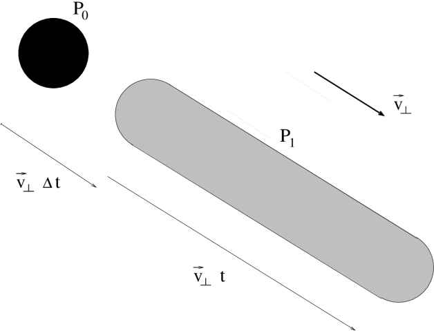
Figure 5: Illustration of the relative positions of the outgoing power and echo power in the scheme described in Section 5.5. The figure is drawn in a reference frame where the outgoing power source is at rest and where a perfectly cold axion fluid moves with velocity $\vec{v}$. If the outgoing power $P_{0}$ is emitted in the direction perpendicular to the plane of the figure from the area of the black circle for a time $t$ and is then turned off, echo power $P_{1}$ arrives in the grey area at a time $\Delta t$ after the outgoing power was turned off. The echo power lasts forever but moves away from the source of outgoing power with velocity $\vec{v}_{\perp}$ where $\vec{v}_{\perp}$ is the component of $\vec{v}$ transverse to the direction of emission of the outgoing power.

returns forever to the location in the axion fluid rest frame from which the increment $dE_{0}$ of outgoing energy was emitted. In the rest frame of the outgoing power source, the echo from outgoing power emitted a time $t_{e}$ ago arrives displaced from the point of emission of the outgoing power by $\vec{d}=\vec{v}_{\perp}t_{e}$ where $\vec{v}_{\perp}$ is the component of $\vec{v}$ perpendicular to the direction $\hat{k}$ of emission. Fig. 5 illustrates the relative locations of the outgoing power and echo power in case the outgoing power is turned on for a while and then turned off. The echo moves away from the place of emission of the outgoing power with velocity $\vec{v}_{\perp}$. To detect as much echo power as possible at or near the place of emission of the outgoing power, the observer wants $\vec{v}_{\perp}$ as small as possible, i.e. $\hat{k}$ in the same direction as $\vec{v}$ or the opposite direction. In the frame of its source, the angular frequency at which the outgoing power stimulates axion decay is

$$\omega_{0}={m_{a}\over 2}(1+\vec{v}\cdot\hat{k})+{\cal O}(v^{2})$$ (138)

whereas

$$\omega_{1}={m_{a}\over 2}(1-\vec{v}\cdot\hat{k})+{\cal O}(v^{2})~{}~{}\ .$$ (139)

is the angular frequency of the echo.

An attractive target for the echo method is the Big Flow, the locally prominent cold dark matter flow in the caustic ring model of the Milky Way halo. Its velocity vector $\vec{v}_{\rm BF}$ in a non-rotating galactic reference frame is given in Eq. (19). In a reference frame attached to the surface of the Earth its velocity is

$$\vec{v}(t)=\vec{v}_{\rm BF}-\vec{v}_{\rm LSR}-\vec{v}_{\odot}-\vec{v}_{\otimes}(t)$$ (140)

where $\vec{v}_{\rm LSR}$ is the velocity of the Local Standard of Rest (LSR) in that same reference frame, $\vec{v}_{\odot}$ is the velocity of the Sun with respect to the LSR, and $\vec{v}_{\otimes}$ is the velocity of the observer with respect to the Sun as a result of the orbital and rotational motions of the Earth. We are particularly interested in the extent to which the uncertainties in the several terms on the RHS of Eq. (140) affect our ability to minimize $\vec{v}_{\perp}$. $\vec{v}_{\otimes}(t)$ is known with great precision. The components of $\vec{v}_{\odot}$ are known with a precision of order two or three km/s. $\vec{v}_{\rm LSR}$ is in the direction of galactic rotation by definition. Its magnitude (often quoted to be 220 km/s) is known within an uncertainty of order 20 km/s. The magnitude of $\vec{v}_{\rm BF}$ scales with the magnitude of $\vec{v}_{\rm LSR}$ and has been estimated to be approximately 520 km/s Duffy and Sikivie (2008). The direction of $\vec{v}_{\rm BF}$ is mostly in the direction of galactic rotation [see Eq. (19)] and is known with a precision of order $1^{\circ}$ Chakrabarty et al. (2020). So we expect that it is possible to reduce $|\vec{v}_{\perp}|$ to approximately 5 km/s, the nominal value we use below.

Consider a dish (e.g. a radiotelescope) of radius $R$ collecting echo power near the location of the outgoing power source. Because the echo from outgoing power emitted a time $t_{e}$ ago is displaced by $\vec{d}=\vec{v}_{\perp}t_{e}$, the amount of echo power collected by the dish is

$$P_{c}={1\over 16}g^{2}\rho{dP_{0}\over d\nu}C{R\over|\vec{v}_{\perp}|}$$ (141)

where $C$ is a number of order one which depends on the configuration of the source relative to the receiver dish:

$$C={|\vec{v}_{\perp}|\over 2RP_{0}}\int dt\int_{S_{0}}d^{2}x~{}I_{0}(\vec{x})\Theta_{c}(\vec{x}+\vec{v}_{\perp}t)~{}~{}\ .$$ (142)

Here $S_{0}$ is the surface from which the outgoing power is emitted, $I_{0}(\vec{x})$ is the outgoing power per unit surface, and $\Theta_{c}(\vec{x})$ is a function that equals one if $\vec{x}$ belongs to the receiver dish area and zero otherwise. For example, $C=0.5$ if the outgoing power is emitted from the center of the receiver dish, whereas $C=0.424$ if the outgoing power is emitted uniformly from the area of the receiver dish. However neither of these configurations is likely to be optimal. It is probably better to place several source dishes around the receiver dish. $C$ can be straightforwardly calculated for each configuration.

Let us assume that a pulse of outgoing power $P_{0}$, with frequency $\nu_{0}$ and uniform spectral density ${dP_{0}\over d\nu}={P_{0}\over\Delta\nu_{0}}$ over bandwidth $\Delta\nu_{0}$, is emitted during a time $t_{m}$. Provided that

$$t_{m}\mathrel{\raise 1.29167pt\hbox{$>$\kern-10.50005pt\lower 4.30554pt\hbox{ $\sim$}}}{R\over 2|\vec{v}_{\perp}|}=0.5\times 10^{-2}~{}{\rm sec}~{}{R\over 50~{}{\rm m}}~{}{5~{}{\rm km/s}\over|\vec{v}_{\perp}|}$$ (143)

echo power

$$P_{c} = 2.33\times 10^{-31}P_{0}\left({10~{}{\rm kHz}\over\Delta\nu_{0}}\right)\left({g_{\gamma}\over 0.36}\right)^{2}\left({10^{12}~{}{\rm GeV}\over f_{a}}\right)^{2}\cdot$$ (144)

$$\cdot \left({\rho\over{\rm GeV/cm}^{3}}\right)\left({C\over 0.30}\right)\left({R\over 50~{}{\rm m}}\right)\left({5~{}{\rm km/s}\over|\vec{v}_{\perp}|}\right)~{}~{}\ ,$$

is received over the same time interval $t_{m}$. Since the magnitude of the velocity of the Big Flow relative to us $v\simeq$ 520 km/s - 220 km/s = 300 km/s, the frequency of the echo power is red- or blue-shifted from $\nu_{0}$ by $\Delta\nu\simeq 2\times 10^{-3}\nu_{0}$. The echo power has bandwidth $B=2\delta v~{}\nu<5\times 10^{-7}\nu$ since the velocity dispersion of the Big Flow is less than 70 m/s Banik and Sikivie (2016). The frequency range of interest is approximately 30 MHz to 30 GHz because the Earth’s atmosphere is mostly transparent at those frequencies. It corresponds to the mass range $2.5\times 10^{-7}<m_{a}<2.5\times 10^{-4}$ eV, which happens to be prime hunting ground for QCD axions.

The cosmic microwave background and radio emission by astrophysical sources are irreducible sources of noise. In addition there is instrumental noise. The total noise temperature depends on frequency, on the location of the telescope and on the direction of observation. As an example we may consider the system noise temperature of the Green Bank Telescope : approximately 20 K from 1 GHz to 8 GHz, approximately linearly rising from 20 K at 8 GHz to 40 K at 30 GHz, and exponentially rising towards low frequencies from 20 K at 1 GHz to 100 K at 300 MHz. The rise at low frequencies is due to Galactic emission and is strongly direction dependent. 100 K at 300 MHz is a typical value. The rise at high frequencies is due to atomic and molecular transitions in the atmosphere. It can be mitigated by placing the telescope at a high elevation. We use below a nominal system noise temperature of 20 K at all frequencies for the purpose of stating the results of our sensitivity calculations.

The signal to noise ratio with which the echo power is detected when $\omega_{0}$ falls within the angular frequency range of the emitted power is given by Dicke’s radiometer equation (73). Combining Eqs. (144) and (73) and setting $B=5\times 10^{-7}\nu$, the total outgoing energy per logarithmic frequency interval necessary to detect the axion echo with a given signal to noise ratio is found to be:

$${dE_{0}\over d\ln\nu}\Bigg{|}_{\rm BF} = 7.2~{}{\rm MWyear}\left({s/n\over 5}\right)\left({10~{}{\rm GHz}\over\nu}\right)^{1\over 2}\left({0.36\over g_{\gamma}}\right)^{2}\left({T_{n}\over 20~{}{\rm K}}\right)\left({{\rm GeV/cm}^{3}\over\rho}\right)\cdot$$ (145)

$$\cdot \left({0.30\over C}\right)\left({t_{m}\over 10^{-2}~{}{\rm sec}}\right)^{1\over 2}\left({50~{}{\rm m}\over R}\right)\left({|v_{\perp}|\over 5~{}{\rm km/s}}\right)\ .$$

We used Eq. (3) and $m_{a}=4\pi\nu$.

General axion fluid

In the most general case, the axion fluid is moving with respect to the observer and has velocity dispersion. Its density can be expressed as an integral over cold flows

$$\rho=\int d^{3}v~{}{d^{3}\rho\over dv^{3}}(\vec{v})~{}~{}\ .$$ (146)

Everything said in the previous subsection holds true for each infinitesimal cold flow increment. The echo frequency has a spread $\delta\omega_{-}={m\over 2}\delta v_{\parallel}$ where $\delta v_{\parallel}$ is the spread of axion velocities in the $\hat{k}$ direction. The echo of power emitted a time $t_{e}$ ago is spread over a transverse size $\delta\vec{d}=\delta\vec{v}_{\perp}t_{e}$ where $\delta\vec{v}_{\perp}$ is the spread of axion velocities perpendicular to $\hat{k}$.

Let us consider the isothermal model of the Milky Way in particular. According to it, the dark matter has density 300 MeV/cm³ on Earth. Its velocity distribution is Gaussian and isotropic in a non-rotating galactic reference frame with dispersion $\sqrt{\vec{v}\cdot\vec{v}}$ = 270 km/s $\equiv\sqrt{3}\sigma$. In the LSR, the axion fluid moves with speed 220 km/s in the direction opposite to that of galactic rotation. Assuming the direction $\hat{k}$ of the outgoing power is parallel (anti-parallel) to the direction of galactic rotation the echo power is blue (red)-shifted in frequency by a fractional amount whose average is $\langle{\Delta\nu\over\nu}\rangle\simeq$ 440 km/s = $1.47\times 10^{-3}$ and whose rms deviation is ${\delta\nu\over\nu}=2\sigma\simeq 1.04\times 10^{-3}$. The echo from outgoing energy that was emitted a time $t_{e}$ ago is spread in space over a fuzzy circular region whose radius is Gaussian-distributed with average value $\sigma t_{e}$. Eq. (141) holds with ${1\over|\vec{v}_{\perp}|}$ replaced by

$$\langle{1\over|\vec{v}_{\perp}|}\rangle=\sqrt{\pi\over 2}{1\over\sigma}={1\over 124~{}{\rm km/s}}~{}~{}\ .$$ (147)

In view of Eq. (143) we now require $t_{m}>2\times 10^{-4}{\rm sec}{R\over 50~{}{\rm m}}$. Using Eq. (73) with $B=4\sigma\nu=2.1\times 10^{-3}\nu$ and setting $\rho$ = 0.3 GeV/cm³, we find

$${dE_{0}\over d\ln\nu}\Bigg{|}_{\rm iso}=5.3~{}{\rm GWyear}\left({s/n\over 5}\right)\left({10~{}{\rm GHz}\over\nu}\right)^{1\over 2}\left({0.36\over g_{\gamma}}\right)^{2}\cdot$$

$$\cdot\left({T_{n}\over 20~{}{\rm K}}\right)\left({0.30\over C}\right)\left({t_{m}\over 2\cdot 10^{-4}~{}{\rm sec}}\right)^{1\over 2}\left({50~{}{\rm m}\over R}\right)\ .$$ (148)

In case of a known cold flow, the echo method appears an attractive approach because it uses relatively old technology and is applicable over a wide range of axion masses.

VI Solar axion detection

The solar axion flux presents an attractive search opportunity. It has been pursued using a number of methods. Eqs. (15) and (16) provide an estimate of the flux on Earth of axions produced in the Sun by the Primakoff process.

VI.0.1 The axion helioscope

Solar axions can be searched for by converting them to photons in a magnetic field Sikivie (1983, 1985); Van Bibber et al. (1987); see Section 3. Multiplying the axion flux by the conversion probability Eq. (49) yields the photon flux

$$\Phi_{\gamma}={0.79\over{\rm cm}^{2}~{}{\rm day}}\left({g_{a\gamma\gamma}\over 10^{-10}~{}{\rm GeV^{-1}}}\right)^{4}\left({L\over 10~{}{\rm m}}\right)^{2}\left({B_{0}\over 10~{}{\rm T}}\right)^{2}$$ (149)

for the case $qL<<1$, $\epsilon=\mu=1$. The photons produced are x-rays with approximately 4 keV average energy. They point back to the solar core. If a signal is found, it becomes possible to see directly into the solar interior. The inverse of the momentum transfer in the axion-photon conversion process is

$${1\over q}\simeq{2E\over m_{a}^{2}}=15.8~{}{\rm m}\left({10^{-2}~{}{\rm eV}\over m_{a}}\right)^{2}\left({E\over 4~{}{\rm keV}}\right)~{}~{}~{}~{}~{}\ .$$ (150)

The resonance condition $qL<1$ is satisfied in vacuum for axion masses up to approximately $1.5\cdot 10^{-2}$ eV if, for example, $L=10$ m. One may extend this range by introducing gas under pressure in the conversion region Van Bibber et al. (1987), giving the photon an effective mass equal to the plasma frequency $\omega_{\rm pl}$. Alternatively one may make the magnetic field periodic with wavelength $d={2\pi\over q}$.

Axion helioscope experiments have been carried out at Brookhaven National Laboratory Lazarus et al. (1992), at the University of Tokyo Moriyama et al. (1998); Inoue et al. (2002, 2008), and by the CAST collaboration at CERN Zioutas et al. (2005); Andriamonje et al. (2007); Arik et al. (2009); Anastassopoulos et al. (2017a). New experiments have been proposed by the IAXO Armengaud et al. (2019); Dafni et al. (2019) and TASTE Anastassopoulos et al. (2017b) collaborations. The Tokyo helioscope magnet (2.3 m long, 4 T field) was mounted on a platform which allowed the Sun to be tracked at all times. The CAST magnet tracks the Sun for only part of the day, approximately 1.5 hour during sunrise and 1.5 hour during sunset, but is longer (9.3 m) and more powerful (9 T). Both experiments have introduced He gas in the conversion region to extend the search range upwards in axion mass Inoue et al. (2008); Arik et al. (2014, 2015). The limits obtained by the CAST and Tokyo experiments are shown in Fig. 6, in rough outline. For details, see the original publications. Additional limits on axion couplings were obtained by the CAST Collaboration Andriamonje et al. (2009, 2010) from a search for mono-energetic axions emitted in nuclear M1 transitions in the Sun. Axion emission rates in the M1 transitions of ⁵⁷Fe, ⁵⁵Mn and ²³Na were calculated in ref. Haxton and Lee (1991).

It has been proposed to search for solar axions converting to x-rays in the magnetic field of the Earth Davoudiasl and Huber (2006) or that of the Sun Hong et al. (2019) using an x-ray detector placed in orbit around the Earth or Sun.

VI.0.2 Axioelectric and Mössbauer effects

Solar axions may be searched for using the axioelectric effect, which is the same as the photoelectric effect but with an axion instead of a photon. It uses the coupling of the axion to the electron. Through this coupling, axions are produced in the Sun by axion bremstrahlung, Compton-like scattering and axion recombination. Theoretical discussions of the axioelectric effect are given in refs. Zhitnitsky and Skovpen (1979); Dimopoulos et al. (1986); Derevianko et al. (2010). Results from experimental searches are reported in refs. Avignone et al. (1987); Ljubicic et al. (2004); Avignone (2009); Bellini et al. (2012); Armengaud et al. (2013); Abe et al. (2013); Alessandria et al. (2013); Derbin et al. (2013); Aprile et al. (2014); Liu et al. (2017); Akerib et al. (2017); Fu et al. (2017); Wang et al. (2020). The bounds on the electron coupling obtained by these searches are of order

$$g_{a\bar{e}e}=g_{e}{m_{e}\over f_{a}}\mathrel{\raise 1.29167pt\hbox{$<$\kern-10.50005pt\lower 4.30554pt\hbox{ $\sim$}}}10^{-11}~{}~{}\ .$$ (151)

The most severe limit reported is $3.5\cdot 10^{-12}$ (90% CL) Akerib et al. (2017).

Solar axions may also be searched for using the Mössbauer effect de Rujula and Zioutas (1989); Moriyama (1995). Nearly monochromatic axions are emitted in nuclear transitions in the Sun, e.g. 14.4 keV axions in transitions between the first excited and ground states of ⁵⁷Fe. Such axions may be searched for by resonant absorption on the same nucleus on Earth. The nucleus emits an x-ray when it de-excites. The process uses the coupling of axions to nucleons. An experimental search of this type is reported in ref. Krcmar et al. (2001).

VI.0.3 Primakoff effect

Solar axions may be searched for by converting them to photons in the Coulomb field of nuclei, i.e. the Primakoff effect. The cross-section for Primakoff conversion of an axion to a photon in the Coulomb field of a nucleus can be obtained by repeating the steps of Section 3.2 but keeping the first term in $\vec{j}_{a}=g(\vec{E}_{0}\times\vec{\nabla}a-\vec{B}_{0}\partial_{t}a)$ instead of the second term, and setting $E_{0}(\vec{x})=Ze\vec{x}/4\pi|\vec{x}|^{3}$. For $\epsilon=\mu=1$, this yields

$${d\sigma\over d\Omega}={g^{2}Z^{2}\alpha\over 4\pi\beta_{a}}{\omega^{2}\over q^{4}}(q^{2}-(\hat{n}\cdot\vec{q})^{2})$$ (152)

where $\vec{q}=\vec{k}-\vec{k}_{a}$, $\vec{k}_{a}=\omega\vec{\beta}_{a}$ is the initial axion momentum and $\vec{k}=\omega\hat{n}$ the final photon momentum. The conversion rate on nuclei forming a crystal lattice is resonantly enhanced when the Bragg scattering condition is satisfied Paschos and Zioutas (1994). As the Earth spins, the varying orientation of the detector with respect to direction of the Sun produces a distinctive temporal pattern of the counting rate, which helps to distinguish signal from background. Searches of this type have been carried out by the SOLAX collaboration Avignone et al. (1998) in Sierra Grande, Argentina, the DAMA collaboration Bernabei et al. (2001) in the Gran Sasso Laboratory, Italy, the COSME collaboration Morales et al. (2002) in the Canfranc Laboratory, Spanish Pyrenees, and the CDMS collaboration Ahmed et al. (2009) in the Soudan Underground Laboratory in Minnesota. The limits obtained are shown in Fig. 6.

VII Dichroism and birefrigence in a magnetic field

The existence of an axion field causes the vacuum to be birefrigent and dichroic in the presence of a magnetic field Maiani et al. (1986); Raffelt and Stodolsky (1988). The purpose of this section is to derive these properties. A medium is called “birefringent” if it has different indices of refraction for the two states of linear polarization of light. It is “dichroic” if it has different absorption coefficients for those two states. In general, light traveling in the $z$-direction has amplitude

$$\vec{A}=Re[({\cal A}_{x}\hat{x}+{\cal A}_{y}\hat{y})e^{-i\omega t}]$$ (153)

where ${\cal A}_{x}$ and ${\cal A}_{y}$ are complex numbers. Eq. (153) implies that, as a function of time $t$, the vector $\vec{A}$ describes an ellipse in the $xy$-plane. By definition, the ellipticity of the light is the ratio of the minor to major axes of that ellipse. If the light is linearly polarized, ${\cal A}_{x}$ and ${\cal A}_{y}$ have the same phase, and we may write $~{}~{}{\cal A}_{x}={\cal A}\cos\alpha~{},~{}{\cal A}_{y}={\cal A}\sin\alpha~{}~{}$ where $\alpha$ is the angle of the plane of polarization with the $x$-axis. The ellipticity of such light is zero. When light that is initially linearly polarized travels through a birefringent material, the relative phase between ${\cal A}_{x}$ and ${\cal A}_{y}$ changes and the light acquires ellipticity. When light that is initially linearly polarized travels through a dichroic material, the plane of polarization rotates towards the direction with least absorption.

Let us recall that, even if there is no axion, the vacuum is birefringent in the presence of a magnetic field as a consequence of the box diagram of quantum electrodynamics. Euler and Heisenberg showed that it implies the effective interaction Heisenberg and Euler (1936); Itzykson and Zuber (1980):

$${\cal L}_{\rm EH}={2\alpha^{2}\over 45m_{e}^{4}}\left[(E^{2}-B^{2})^{2}+7(\vec{E}\cdot\vec{B})^{2}\right]~{}~{}~{}\ ,$$ (154)

as a consequence of which light traveling through a magnetic field $\vec{B}_{0}$ has different indices of refraction depending on whether it is polarized parallel or perpendicular to $\vec{B}_{0}$.

Let us assume that an axion exists and consider light traveling in the $\hat{z}$ direction in a constant magnetic field $\vec{B}=B_{0}\hat{x}$, and initially linearly polarized ($\vec{A}_{\rm in}$) at an angle $\alpha$ relative to the direction of the magnetic field. See Fig. 7. In view of Section 3, we expect the $x$-component of light to become depleted by $\gamma\rightarrow a$ conversion whereas the $y$-component propagates as usual. Specifically, after a distance $L$, the magnitude of the $x$ component of light is reduced $~{}~{}|{\cal A}_{x}|\rightarrow(1-{1\over 2}p(L))|{\cal A}_{x}|$, where $p(L)$ is the conversion probability given in Eq. (44), whereas $|{\cal A}_{y}|$ is unchanged. The plane of polarization rotates therefore by the angle

$$\delta\alpha(L)={1\over 4}~{}p(L)~{}\sin(2\alpha)~{}~{}~{}\ .$$ (155)

In addition the light acquires ellipticity because the relative phase between ${\cal A}_{x}$ and ${\cal A}_{y}$ changes Maiani et al. (1986); Raffelt and Stodolsky (1988), i.e.

$${\cal A}_{y}\rightarrow{\cal A}_{y}~{}~{}~{}~{},~{}~{}~{}~{}{\cal A}_{x}\rightarrow[1-{1\over 2}p(L)+i\phi(L)]{\cal A}_{x}~{}~{}~{}\ .$$ (156)

In terms of $\phi(L)$, the acquired ellipticity is

$$e(L)={1\over 2}|\phi(L)|\sin(2\alpha)~{}~{}~{}\ .$$ (157)

Thus, if an axion exists, there is dichroism and a new source of birefringence in the presence of a magnetic field. We now derive the expression for the phase shift $\phi(L)$ Maiani et al. (1986). As a byproduct, Eq (44) for the conversion probability $p(L)$ will be rederived Maiani et al. (1986); Raffelt and Stodolsky (1988) as well.

Consider a region of homogeneous dielectric constant $\epsilon$ and homogeneous static external magnetic field $\vec{B}_{0}$. Axion-photon dynamics in such a region is described by the modified Maxwell’s equations

$$\epsilon\vec{\nabla}\cdot\vec{E} = g\vec{B}_{0}\cdot\vec{\nabla}a$$

$$\vec{\nabla}\times\vec{B}-\epsilon\partial_{t}\vec{E} = -g\vec{B}_{0}\partial_{t}a$$ (158)

and the equation of motion for the axion field

$$(\partial_{t}^{2}-\vec{\nabla}^{2}+m_{a}^{2})a=-g\vec{B}_{0}\cdot\vec{E}~{}~{}~{}~{}~{}\ .$$ (159)

We choose the gauge $\Phi=0$. Any solution of Eqs. (158,159) is a linear superposition of plane waves:

$$\vec{\cal A}(\vec{x},t)=\vec{\cal A}~{}e^{i(\vec{k}\cdot\vec{x}-wt)}~{}~{}~{}~{},~{}~{}~{}~{}~{}{\bf a}(\vec{x},t)={\bf a}~{}e^{i(\vec{k}\cdot\vec{x}-wt)}~{}~{}~{}~{}~{}\ ,$$ (160)

where the relation between $\omega$ and $\vec{k}$ depends on the direction of polarization. Let $\vec{k}=k\hat{z}$ and

$$\vec{B}_{0}=B_{0z}~{}\hat{z}+B_{0x}~{}\hat{x}~{}~{}~{}~{},~{}~{}~{}~{}\vec{\cal A}={\cal A}_{z}~{}\hat{z}+{\cal A}_{x}~{}\hat{x}+{\cal A}_{y}~{}\hat{y}~{}~{}~{}~{}\ .$$ (161)

Eqs. (158,159) are equivalent to:

$$i\omega\epsilon{\cal A}_{z} = +gB_{0z}{\bf a}$$

$$(k^{2}-\epsilon\omega^{2}){\cal A}_{y} = 0$$ (162)

and

$$k^{2}\Biggl{(}{{\cal A}_{x}\atop{\bf a}}\Biggr{)}=\Biggl{(}\matrix{\epsilon\omega^{2}&+igB_{0x}\omega\cr-igB_{0x}\omega&\omega^{2}-m_{a}^{2}-{1\over\epsilon}g^{2}B_{0z}^{2}}\Biggr{)}\Biggl{(}{{\cal A}_{x}\atop{\bf a}}\Biggr{)}~{}~{}~{}~{}\ .$$ (163)

Thus the $A_{y}$ mode propagates in the usual fashion, whereas the $A_{x}$ mode oscillates into the axion field and vice-versa. From Eq. (163), one finds the $k^{2}$-eigenvalues for given $\omega$

$$k_{\pm}^{2}={1\over 2}\left[(\epsilon+1)\omega^{2}-m_{a}^{2}-{(gB_{0z})^{2}\over\epsilon}\pm\sqrt{\Bigl{(}(\epsilon-1)\omega^{2}+m_{a}^{2}+{(gB_{0z})^{2}\over\epsilon}\Bigr{)}^{2}+4g^{2}B_{0x}^{2}\omega^{2}}~{}\right]~{}~{}~{}~{}\ .$$ (164)

The corresponding eigenmodes are proportional to:

$$\Biggl{(}{{\cal A}_{x}\atop{\bf a}}\Biggr{)}_{\pm}\equiv\Biggl{(}{-igB_{0x}\omega\atop\epsilon\omega^{2}-k_{\pm}^{2}}\Biggr{)}~{}~{}~{}~{}\ .$$ (165)

The general solution is therefore:

$${\cal A}_{y} = ({\cal A}_{y+}~{}e^{ikz}+{\cal A}_{y-}~{}e^{-ikz})e^{-i\omega t}$$

$$\Biggl{(}{{\cal A}_{x}\atop{\bf a}}\Biggr{)} = \Biggl{[}\Biggl{(}{\cal A}_{++}e^{ik_{+}z}+{\cal A}_{+-}e^{-ik_{+}z}\Biggr{)}\Biggl{(}{{\cal A}_{x}\atop{\bf a}}\Biggr{)}_{+}$$ (166)

$$+ \Biggl{(}{\cal A}_{-+}e^{ik_{-}z}+{\cal A}_{--}e^{-ik_{-}z}\Biggr{)}\Biggl{(}{{\cal A}_{x}\atop{\bf a}}\Biggr{)}_{-}\Biggr{]}e^{-i\omega t}~{}~{}~{}~{}\ .$$

where ${\cal A}_{y\pm},~{}{\cal A}_{+\pm}$ and ${\cal A}_{-\pm}$ are constants, and $k=\sqrt{\epsilon}\omega$.

We are interested in the solution describing a wave traveling in the $+\hat{z}$ direction which is initially, at z=0, a purely electromagnetic wave linearly polarized at an angle $\alpha$ relative to $\hat{x}$. For that case

$${\cal A}_{y-} = {\cal A}_{+-}={\cal A}_{--}=0$$

$${\cal A}_{y}|_{z=0} = {\cal A}~{}\sin\alpha~{}e^{-i\omega t}~{}~{}~{},~{}~{}~{}{\cal A}_{x}|_{z=0}={\cal A}~{}\cos\alpha~{}e^{-i\omega t}~{}~{}~{},~{}~{}~{}~{}{\bf a}|_{z=0}=0$$ (167)

and therefore

$$A_{y}(z,t) = Re[{\cal A}\sin\alpha~{}e^{i(kz-\omega t)}]$$

$$A_{x}(z,t) = Re\left[{{\cal A}\cos\alpha\over k_{+}^{2}-k_{-}^{2}}\left((\epsilon\omega^{2}-k_{-}^{2})~{}e^{i(k_{+}z-\omega t)}-(\epsilon\omega^{2}-k_{+}^{2})~{}e^{i(k_{-}z-\omega t)}\right)\right]$$

$$a(z,t) = Re\left[-i{\cal A}\cos\alpha~{}{gB_{0x}\omega\over k_{+}^{2}-k_{-}^{2}}\left(e^{i(k_{+}z-\omega t)}-e^{i(k_{-}z-\omega t)}\right)\right]~{}~{}~{}~{}\ .$$ (168)

We used the identity $(\epsilon\omega^{2}-k_{-}^{2})(\epsilon\omega^{2}-k_{+}^{2})=-g^{2}B_{0x}^{2}\omega^{2}$. From Eqs. (168) one may obtain the energy fluxes in the axion field ${\cal P}_{a}(z)=<-\partial_{t}a\partial_{z}a>$ and in each polarization state of the photon field: ${\cal P}_{x}(z)=<-\partial_{t}A_{x}\partial_{z}A_{x}>$ and ${\cal P}_{y}(z)=<-\partial_{t}A_{y}\partial_{z}A_{y}>$. The brackets indicate time averages. The $a\rightarrow\gamma$ conversion probability is found to be:

$$p(z)={{\cal P}_{a}(z)\over{\cal P}_{x}(0)}={4g^{2}B_{0x}^{2}\omega^{2}\sin^{2}({(k_{+}-k_{-})z\over 2})\over(k_{+}^{2}-k_{-}^{2})^{2}}\left(1+{\cal O}({k_{+}-k_{-}\over k})\right)~{}~{}~{}\ .$$ (169)

Since

$$gB_{0}={\alpha\over\pi}{g_{\gamma}\over f_{a}}B_{0}=1.63~{}10^{-16}~{}{\rm eV}\Biggl{(}{10^{7}~{}{\rm GeV}\over f_{a}}\Biggr{)}\Biggl{(}{B_{0}\over 10~{}{\rm T}}\Biggr{)}\Biggl{(}{g_{\gamma}\over 0.36}\Biggr{)}~{}~{}~{}~{}\ ,$$ (170)

$(gB_{0})^{2}$ is much smaller than $\epsilon\omega^{2}$ and $\omega^{2}-m_{a}^{2}$ in most cases of practical interest. If so, Eq. (164) becomes

$$k_{+}^{2} = \epsilon\omega^{2}+{g^{2}B_{0x}^{2}\omega^{2}\over(\epsilon-1)\omega^{2}+m_{a}^{2}}+{\cal O}(g^{4}B_{0}^{4})$$

$$k_{-}^{2} = \omega^{2}-m_{a}^{2}-{g^{2}B_{0z}^{2}\over\epsilon}-{g^{2}B_{0x}^{2}\omega^{2}\over(\epsilon-1)\omega^{2}+m_{a}^{2}}+{\cal O}(g^{4}B_{0}^{4})~{}~{}~{}~{}~{}\ .$$ (171)

We have then

$$p(z)={g^{2}B_{0x}^{2}\over\epsilon q^{2}}\sin^{2}({qz\over 2})~{}\left(1+{\cal O}(g^{2}B_{0}^{2},{q\over k})\right)~{}~{}~{}~{}~{}\ ,$$ (172)

where

$$q=\sqrt{\epsilon}\omega-\sqrt{\omega^{2}-m_{a}^{2}}~{}~{}~{}~{}\ .$$ (173)

Eq. (172) agrees with Eq. (44) on resonace, i.e. when $q\rightarrow 0$ and hence $\beta_{a}\rightarrow\sqrt{\epsilon}$. Rewriting the second Eq. (168) in the form

$$A_{x}=Re[{\cal A}\cos\alpha~{}(1+\delta(z)+i\phi(z))~{}e^{i(kz-\omega t)}]~{}~{}\ ,$$ (174)

we find $\delta(z)=-{1\over 2}p(z)$ as anticipated, and Maiani et al. (1986); Raffelt and Stodolsky (1988)

$$\phi(z)={g^{2}B_{0x}^{2}\over 4\epsilon q^{2}}\left(qz-\sin(qz)\right)~{}\left(1+{\cal O}(g^{2}B_{0}^{2},{q\over k})\right)~{}~{}~{}~{}\ ,$$ (175)

for the phase shift.

Dichroism and birefringence of the vacuum in the presence of a magnetic field was searched for by the RBFT collaboration at Brookaven National Laboratory Cameron et al. (1993) and by the PVLAS collaboration at the INFN National Laboratory in Legnaro, Italy Zavattini et al. (2006, 2008). The sensitivity to optical rotation achieved in these experiments is of order $10^{-8}$ radians. The Cotton-Mouton and Voigt effects are important backgrounds. The Cotton-Mouton effect is the birefringence of liquids in the presence of a magnetic field transverse to the direction of propagation. The Voigt effect is the analogous effect in gases. The signal is enhanced by the use of an optical cavity which allows the laser beam to be passed through the magnetic field many times. Eq. (155) is replaced in that case by

$$\delta\alpha(L)={1\over 4}p(L)\sin(2\alpha)N$$ (176)

where $N$ is the number of passes through the magnet. With $N\sim 10^{5}$, $B\sim$ few Tesla, and $L\sim 10$ m, the sensitivity in $g$ is of order $(10^{7}~{}{\rm GeV})^{-1}$ when the resonance condition $qL<1$ is satisfied. For laser light ($\omega\sim$ eV) in vacuum ($\epsilon$ = 1), and $L\sim$ 10 m, the resonance condition is satisfied when $m_{a}\mathrel{\raise 1.29167pt\hbox{$<$\kern-10.50005pt\lower 4.30554pt\hbox{ $\sim$}}}$ 0.3 meV. For $m_{a}>$ meV, the sensitivity to $g$ decreases as $m_{a}^{-2}$. The PVLAS collaboration claimed a signal in ref. Zavattini et al. (2006) but retracted it after additional measurements were made Zavattini et al. (2008).

Refs. Zarei et al. (2019); Shakeri et al. (2020) propose schemes to measure the birefringence of light due to virtual axion exchange in a magnetic field or in a high intensity laser beam.

VIII Shining light through walls

Another approach to axion detection is $\gamma\rightarrow a$ conversion in a magnetic field followed by $a\rightarrow\gamma$ back-conversion, also in a magnetic field Van Bibber et al. (1987). This type of experiment is commonly referred to as “shining light through walls”. If $P_{0}$ is the power of the laser, and $p$ and $p^{\prime}$ the conversion probabilities in the magnets on the left and right hand side of the wall, the power in regenerated photons is $P=p^{\prime}~{}p~{}P_{0}$. Formulas for the conversion probabilities can be found in Section 3. Shining light through walls experiments have been carried out by several groups Ruoso et al. (1992); Robilliard et al. (2007); Pugnat et al. (2008); Chou et al. (2008); Afanasev et al. (2008); Ehret et al. (2010); Ballou et al. (2015). For $m_{a}<3\cdot 10^{-4}$ eV, the following limit on the axion coupling to two photons has been obtained Ballou et al. (2015)

$$g_{a\gamma\gamma}<3.5\cdot 10^{-8}~{}{\rm GeV}^{-1}~{}~{}\ .$$ (177)

It is less severe than the limit from the CAST solar axion search Andriamonje et al. (2007). This is due largely to the high intensity of the solar axion flux compared to the flux produced by photon conversion in a laboratory magnetic field, and the fact that solar axions have keV energies whereas axions produced by lasers have eV energies. On the other hand, shining light through walls is a purely laboratory experiment and the simple version described above can be improved upon.

A first improvement is to introduce an optical cavity in which the photons, on the axion production side of the wall, are bounced back and forth multiple times Ruoso et al. (1992). Each photon in the cavity converts to axions with probability $p$ for each pass through the cavity. If the reflectivity of the mirrors is $R=1-\eta$ and $P_{0}$ is the laser power, the power of the right-moving wave in the cavity is ${1\over 2\eta}~{}P_{0}$. The axion power through the wall is then increased by the factor ${1\over 2\eta}$. Presently available mirrors may have $\eta$ as small as $10^{-5}$.

A further improvement Hoogeveen and Ziegenhagen (1991); Fukuda et al. (1996); Sikivie et al. (2007); Mueller et al. (2009) is to have tuned Fabry-Pérot cavities on both sides of the wall. It is shown below that the probability of axion to photon conversion in the reconversion cavity is ${2\over\pi}~{}{\cal F}^{\prime}~{}p^{\prime}$ where ${\cal F}^{\prime}$ is the finesse of the reconversion cavity, and $p^{\prime}$ the reconversion probability in the absence of cavity. The finesse of a cavity is ${\cal F}={\pi\over\eta}$ if the reflectivity of its mirrors is $R=1-\eta$. Including both improvements, the regenerated photon power is

$$P={1\over\eta^{\prime}\eta}~{}p^{\prime}~{}p~{}P_{0}~{}~{}~{}\ .$$ (178)

Half of the power $P$ is right-moving and half is left-moving. To detect all the regenerated photons, detectors should be installed on both sides of the regeneration cavity. We implicitly assumed in Eq. (178) that the loss of power from the regeneration cavity is enirely due to transmission through its mirrors. In general there are other contributions, $\eta^{\prime}=\eta^{\prime}_{\rm trans}+\eta^{\prime}_{abs}+\eta^{\prime}_{scatt}$, where the latter two terms represent absorption and scattering (including diffraction) losses. If transmission is not entirely dominant, the RHS of Eq. (178) is multiplied by the factor $f=\eta^{\prime}_{\rm trans}/\eta^{\prime}$. An experiment of this type, named ALPS II, is presently under construction at DESY Bähre et al. (2013). A derivation Mueller et al. (2009) of Eq. (178) follows.

The modes of a Fabry-Perot cavity are described in $\Phi=0$ gauge by standing waves:

$$\vec{A}=A\hat{x}\sin(kz)\cos(\omega t)$$ (179)

with $k=\sqrt{\epsilon}\omega$. $\epsilon$ is the dielectric constant in the cavity. We set the magnetic permeability $\mu$ = 1 for simplicity. The cavity has mirrors which enforce $E_{x}=0$ at $z=0$ and $z=L$. Thus the wavevector has quantized values: $k={\pi n\over L}$ with $n=1,~{}2,~{}3~{}...$. The energy stored in the cavity is

$$E={1\over 4}SLA^{2}\epsilon\omega^{2}$$ (180)

where $S$ is the transverse area of the standing wave. Eq. (179) assumes $kS>>L$.

When a cavity mode $\vec{A}=\hat{x}A(t)\sin(kz)$ is not driven, its amplitude satisfies

$$({d^{2}\over dt^{2}}+\gamma{d\over dt}+\omega^{2})A(t)=0~{}~{}\ .$$ (181)

The quality factor is $Q={\omega\over\gamma}$. The power in the right-moving component is

$$P_{+}={1\over 8}SA^{2}\sqrt{\epsilon}\omega^{2}~{}~{}~{}~{}\ .$$ (182)

If the mirrors have reflectivity $R=1-\eta$ and there are no other losses, the power emitted through the two mirrors is $2\eta P_{+}=\gamma E$. Hence

$$Q=L{\sqrt{\epsilon}\omega\over\eta}=n{\cal F}$$ (183)

where ${\cal F}$ is the finesse.

In the presence of a large static magnetic field $\vec{B}_{0}$, the inhomogeneous Maxwell’s equations (158) apply. The axion beam traveling through the regeneration cavity is described by

$$a(z,t)=a\sin(k_{a}z-\omega t)~{}~{}~{}~{}\ .$$ (184)

It is assumed to have the same transverse area $S$ as the regeneration cavity mode. In practice, $S$ varies along the beam path. The calculation below assumes that the axion wave and the photon wave in the regeneration cavity follow the profile of the hypothetically unimpeded photon wave in the production cavity. The power in the axion beam is

$$P_{a}=S<-\partial_{t}a~{}\partial_{z}a>={1\over 2}Sa^{2}\omega k_{a}~{}~{}~{}\ .$$ (185)

Let $\vec{B}_{0}=B_{0}\hat{x}$ and $\vec{A}(z,t)=A(z,t)\hat{x}$. The first Eq. (158) is trivially satisfied whereas the second becomes

$$(\epsilon{\partial^{2}\over\partial t^{2}}-{\partial^{2}\over\partial z^{2}})A(z,t)=\omega gB_{0}a\cos(k_{a}z-\omega t)~{}~{}~{}\ .$$ (186)

Since $A(0,t)=A(L,t)=0$, we may expand

$$A(z,t)=\sum_{n=1}^{\infty}A_{n}(t)\sin({n\pi\over L}z)~{}~{}~{}\ .$$ (187)

Substituting back in Eqs. (186) one finds

$$({d^{2}\over dt^{2}}+\omega_{n}^{2})A_{n}(t)=D\sin(\omega t+{qL\over 2})$$ (188)

where $\omega_{n}={n\pi\over\sqrt{\epsilon}L}$ and

$$D={1\over\epsilon}g\omega B_{0}a{2\over Lq}\sin({qL\over 2})~{}~{}~{}\ .$$ (189)

$q=k_{n}-k_{a}={n\pi\over L}-\sqrt{\omega^{2}-m_{a}^{2}}$ is the momentum transfer, as before. Non-resonant terms are neglected. When dissipation is included, Eq. (188) becomes

$$({d^{2}\over dt^{2}}+\gamma{d\over dt}+\omega_{n}^{2})A_{n}(t)=D\sin(\omega t+{qL\over 2})~{}~{}~{}~{}\ .$$ (190)

Up to transients, the solution is

$$A_{n}(t)={D\sin(\omega t-\phi)\over\sqrt{(\omega_{n}^{2}-\omega^{2})^{2}+\omega^{2}\gamma^{2}}}$$ (191)

with

$$\phi=-{qL\over 2}+\tan^{-1}({\omega\gamma\over\omega_{n}^{2}-\omega^{2}})~{}~{}~{}\ .$$ (192)

When the laser cavity and the regeneration cavity are tuned to the same frequency ($\omega_{n}=\omega$)

$$\vec{A}=\hat{x}A\sin({n\pi\over L}z)\sin(\omega t+{qL\over 2}-{\pi\over 2})$$ (193)

with

$$A={D\over\omega\gamma}={gB_{0}a\over\epsilon\gamma}{2\over Lq}\sin({qL\over 2})~{}~{}~{}\ .$$ (194)

The energy $E$ stored in the mode is given by Eq. (180). Dividing the power $\gamma E$ that the cavity emits by the axion power $P_{a}$, one obtains the axion to photon conversion probability

$$p_{\rm FP}={2g^{2}B_{0}^{2}\over\epsilon\beta_{a}\omega L}Q{1\over q^{2}}\sin^{2}({qL\over 2})~{}~{}~{}~{}\ .$$ (195)

In terms of the conversion probablity $p$ in the same region without cavity [Eq. (44) with $\mu=1$] we have

$$p_{\rm FP}={2Q\over\sqrt{\epsilon}L\omega}p={2{\cal F}\over\pi}p~{}~{}~{}~{}\ ,$$ (196)

as announced.

Refs. Hoogeveen (1992); Caspers et al. (2009); Bogorad et al. (2019); Janish et al. (2019) propose ”shining light through walls” using microwaves instead of visible light. Axions are produced in one electromagnetic cavity permeated by a magnetic field and detected in an other.

IX Long range forces mediated by axions

The exchange of virtual axions produces forces between macroscopic bodies that may manifest themselves as deviations from the $1/r^{2}$ gravitational law Moody and Wilczek (1984). It also produces effective interactions in atoms that modify slightly atomic spectroscopy Weinberg (1978).

The general form of the interaction of the axion with a Dirac fermion $f$ is given in Eq. (8). It implies the interaction energy given in Eq. (9) in case the fermion is non-relativistic. It also implies that the fermion is a source for the axion field:

$$(\partial_{t}^{2}-\nabla^{2}+m_{a}^{2})a(\vec{x},t)=+{g_{f}\over 2f_{a}}\vec{\nabla}\cdot[\chi^{\dagger}(\vec{x},t)\vec{\sigma}\chi(\vec{x},t)]+{m_{f}\theta_{f}\over f_{a}}\chi^{\dagger}(\vec{x},t)\chi(\vec{x},t)$$ (197)

where $\chi(\vec{x},t)$ is the non-relativistic fermion’s two-component spinor field. Let us assume that a spin 1/2 fermion is localized at $\vec{x}_{1}$ and that its spin state is slowly varying on the time scale set by $m_{a}^{-1}$. Eq. (197) implies then

$$a(\vec{x}) = {1\over f_{a}}(m_{f}\theta_{f}+{g_{f}\over 2}\vec{\sigma}\cdot\vec{\nabla}){e^{-m_{a}r}\over 4\pi r}$$ (198)

$$= {1\over f_{a}}\left(m_{f}\theta_{f}-{g_{f}\over 2}(\vec{\sigma}\cdot\hat{r})(m_{a}+{1\over r})\right){e^{-m_{a}r}\over 4\pi r}$$

where $\vec{r}=r\hat{r}=\vec{x}-\vec{x}_{1}$ and $\vec{\sigma}$ acts on the fermion spin state. Let us assume further that a second fermion $f^{\prime}$ is localized at $\vec{x}_{2}$. Eq. (9) implies an interaction energy between the two fermions

$$V(\vec{x}_{2}-\vec{x}_{1};\vec{\sigma},\vec{\sigma}^{\prime})={1\over f_{a}}(-m_{f}^{\prime}\theta_{f}^{\prime}+{g_{f}^{\prime}\over 2}\vec{\sigma}^{\prime}\cdot\vec{\nabla}_{2})a(\vec{x}_{2}-\vec{x}_{1})$$ (199)

where primed quantities refer to the second fermion. Substituting Eq. (198) the interaction energy is seen to be the sum of three terms

$$V(\vec{x}_{2}-\vec{x}_{1};\vec{\sigma},\vec{\sigma}^{\prime})~{}=~{}V_{\rm mon-mon}~{}+~{}V_{\rm mon-dip}~{}+~{}V_{\rm dip-dip}~{}~{}~{}\ ,$$ (200)

called ‘monopole-monopole’, ‘monopole-dipole’, and ‘dipole-dipole’ interactions:

$$V_{\rm mon-mon} = -{m_{f}\theta_{f}m_{f}^{\prime}\theta_{f}^{\prime}\over f_{a}^{2}}~{}{e^{-m_{a}r}\over 4\pi r}$$

$$V_{\rm mon-dip} = -{1\over f_{a}^{2}}[m_{f}\theta_{f}g_{f}^{\prime}~{}\vec{r}\cdot\vec{\sigma}^{\prime}-m_{f}^{\prime}\theta_{f}^{\prime}g_{f}~{}\vec{r}\cdot\vec{\sigma}]~{}{e^{-m_{a}r}\over 8\pi r^{2}}(m_{a}+{1\over r})$$

$$V_{\rm dip-dip} = -{g_{f}g_{f}^{\prime}\over 4f_{a}^{2}}~{}\sigma_{j}\sigma^{\prime}_{k}~{}\bigg{(}\delta_{jk}[{e^{-m_{a}r}\over 4\pi r^{2}}(m_{a}+{1\over r})+{1\over 3}\delta^{3}(\vec{r})]$$ (201)

$$- r_{j}r_{k}{e^{-m_{a}r}\over 4\pi r^{3}}(m_{a}^{2}+3{m_{a}\over r}+3{1\over r^{2}})\bigg{)}$$

where $\vec{r}=\vec{x}_{2}-\vec{x}_{1}$.

Relative to the gravitational potential $-{G_{N}m_{f}m_{f}^{\prime}\over r}$, the potential due to axion exchange is enhanced by the factor $\left({M_{\rm Planck}\over f_{a}}\right)^{2}$ but has a finite range $m_{a}^{-1}$. When the coupling $f_{a}^{-1}$ is large, the range $m_{a}^{-1}$ is small, and vice-versa. The monopole-monopole force is at any rate small compared to the gravitational force because it is suppressed by two powers of $\theta_{f}$. Recall that the $\theta_{f}$ are expected to be of order $\theta_{\rm QCD}$ and $\theta_{\rm QCD}$ is less than $10^{-10}$ in view of the upper limit on the neutron electric dipole moment. If there is Peccei-Quinn symmetry and no other physics beyond the Standard Model, $\theta_{\rm QCD}\sim 10^{-17}$ due to CP violation in the weak interactions. The dipole-dipole force is not suppressed by any powers of $\theta_{f}$ and therefore relatively large. It has a background from ordinary magnetic forces but this background can be suppressed to some extent by using superconducting shields. The monopole-dipole force may be the most attractive target as it has only one factor of $\theta_{f}$ and does not have such a large background from ordinary magnetic forces.

The monopole-dipole force has been searched for using a variety of approaches including torsion balance techniques Ritter et al. (1993); Hammond et al. (2007); Hoedl et al. (2011); Terrano et al. (2015), the effect of a large unpolarized mass on a nearby co-magnetometer Youdin et al. (1996); Lee et al. (2018a), its effect on a paramagnetic salt sample Ni et al. (1999); Crescini et al. (2017), the spin relaxation of cold neutrons Ignatovich and Pokotilovski (2009); Serebrov et al. (2010) and ³He nuclei Guigue et al. (2015) due to their collisions with trap walls, the shift in the nuclear spin precession frequency due to the presence of a nearby unpolarized mass Tullney et al. (2013), and the shifts in atomic energy levels due to P and T violating interactions Stadnik et al. (2018). These searches place lower bounds on $f_{a}/\sqrt{\theta_{f}}$ that reach of order $10^{15}$ GeV for ALPs that are massless or sufficiently light Youdin et al. (1996); Tullney et al. (2013); Crescini et al. (2017); Lee et al. (2018a). The bounds do not reach QCD axions because the range of QCD axion mediated forces is too short in all cases.

The dipole-dipole force has been searched for with a variety of approaches as well, including the shifts in nuclear Zeeman frequency Glenday et al. (2008) and nuclear precession frequency Vasilakis et al. (2009) due to proximity with a polarized source, atomic spectroscopy Ledbetter et al. (2013); Ficek et al. (2017), torsion balance techniques Terrano et al. (2015), scanning tunneling microscopy Luo et al. (2017), and the effect of a polarized source on a nearby co-magnetometer Lee et al. (2018b). The resulting lower bounds on $f_{a}$ reach of order $10^{5}$ GeV for ALPs that are massless or sufficiently light Terrano et al. (2015); Lee et al. (2018b). They do not reach QCD axions for the same reason as above.

The ARIADNE experiment Arvanitaki and Geraci (2014) proposes to produce an oscillating axion field by rotating an unpolarized non-axially symmetric macroscopic body at a frequency $\omega$. The axion field produces an effective transverse magnetic field at the location of a nearby sample that is nuclear spin polarized by a laboratory magnetic field adjusted so that its Larmor frequency equals $\omega$. The oscillating axion field then resonantly excites transverse magnetization in the polarized body. The transverse magnetization is detected by a SQUID magnetometer.

X Photon flux from relic axion decay

Through its electromagnetic coupling, the axion decays to two photons at the rate

$$\Gamma_{a\rightarrow 2\gamma}=g_{\gamma}^{2}~{}{\alpha^{2}\over 64\pi^{3}}~{}{m_{a}^{3}\over f_{a}^{2}}\simeq~{}{1.5\cdot 10^{-50}\over{\rm sec}}~{}\left({m_{a}\over 10^{-5}~{}{\rm eV}}\right)^{5}\left({g_{\gamma}\over 0.36}\right)^{2}~{}~{}\ .$$ (202)

One may search for the photon flux from the decay of relic axions Bershady et al. (1991); Ressell (1991); Blout et al. (2001). The signal is largest when the decay rate is of order the Hubble rate today. If the decay rate is much larger, the axions have decayed already. If much less, too few axions are decaying at present. Eq. (202) indicates that the largest signal is for an axion mass of order 10 eV. Such large axion masses are inconsistent with the constraints from laboratory searches and stellar evolution. We may however consider a broader class of axion-like particles (ALPs). We assume the ALP is a light pseudoscalar similar to the axion except that its coupling to two photons $g_{A\gamma\gamma}$ and its mass $m_{A}$ are unrelated. We use the letter $~{}A~{}$ to indicate the ALP field.

The two photon coupling $g_{A\gamma\gamma}$, defined by

$${\cal L}_{A\gamma\gamma}=-g_{A\gamma\gamma}~{}A~{}\vec{E}\cdot\vec{B}~{}~{}~{}\ ,$$ (203)

is bounded from above

$$g_{A\gamma\gamma}<10^{-10}~{}{\rm GeV}^{-1}$$ (204)

by requiring that ALP emission does not excessively shorten the lifetimes of horizontal branch stars in globular clusters Raffelt (2008). In terms of this bound and the present age of the universe, $t_{0}=1.38\cdot 10^{10}$ years, the ALP decay rate is

$$\Gamma_{A\rightarrow 2\gamma}\simeq{1\over t_{0}}\left({g_{A\gamma\gamma}\over 10^{-10}~{}{\rm GeV}^{-1}}\right)^{2}\left({m_{A}\over 310~{}{\rm eV}}\right)^{3}$$ (205)

assuming no other decay modes. ALPs are produced in the early universe through processes analogous to those that produce axions. Both thermal and cold relic ALP populations may occur.

Let us consider an aggregate of relic ALPs of total mass $M$, e.g. all ALPs that are part of a galaxy cluster. The aggregate emits photons with frequency $\omega={1\over 2}m_{A}$. Its luminosity is $L=M\Gamma_{A\rightarrow 2\gamma}$. In a flat static universe, the energy flux observed at a large distance $r$ from the aggregate is $I={L\over 4\pi r^{2}}$. Let $S$ be the cross-sectional area of the aggregate as seen from the direction of the observer, and therefore $\Delta\Omega=S/r^{2}$ the subtended solid angle. We may write

$$M=\int_{S}d^{2}x\int dr~{}\rho_{A}(\vec{r})=\int_{\Delta\Omega}r^{2}d\Omega~{}\Sigma(\hat{n})$$ (206)

where

$$\Sigma(\hat{n})=\int dr~{}\rho_{A}(\vec{r}=r\hat{n})$$ (207)

is the column density in the direction $\hat{n}$. The energy flux per unit solid angle is therefore

$${dI\over d\Omega}(\hat{n})=\Gamma_{A\rightarrow 2\gamma}{dM\over 4\pi r^{2}d\Omega}={1\over 4\pi}\Gamma_{A\rightarrow 2\gamma}~{}\Sigma(\hat{n})~{}~{}\ .$$ (208)

Eq. (208) is valid in a flat static space-time, or on sufficiently small scales in a curved space-time.

We next discuss how these equations are modified in an expanding homogeneous spatially flat universe. The metric is

$$ds^{2}=-dt^{2}+R(t)^{2}d\vec{x}\cdot d\vec{x}$$ (209)

where $R(t)$ is the cosmological scale factor. We assume that both the observer and aggregate occupy fixed positions in comoving coordinates. The light emitted at time $t_{E}$ and observed at time $t_{0}$ travels a distance

$$r=xR(t_{0})=\int_{t_{E}}^{t_{0}}dt~{}{R(t_{0})\over R(t)}$$ (210)

where $x$ is the comoving coordinate distance between the observer and the source. Consider $N$ photons emitted over a small time interval $\Delta t_{E}$ and arriving at the observer over time interval $\Delta t_{0}$. Since

$$x=\int_{t_{E}+\Delta t_{E}}^{t_{0}+\Delta t_{0}}dt~{}{1\over R(t)}$$ (211)

is unchanged, we have

$$\Delta t_{0}=\Delta t_{E}~{}{R(t_{0})\over R(t_{E})}~{}~{}\ .$$ (212)

Therefore the observed photons are redshifted to the angular frequency

$$\omega={m_{A}\over 2}{1\over 1+z_{E}}~{}~{}~{}$$ (213)

where

$$1+z_{E}={R(t_{0})\over R(t_{E})}~{}~{}~{}\ .$$ (214)

Eq. (212) also implies that the $N$ photons arrive at the observer at a rate which is ${1\over 1+z_{E}}$ times the rate at which they are emitted. The observed energy flux is therefore

$$I={\Gamma_{A\rightarrow 2\gamma}~{}M\over 4\pi r^{2}}{1\over(1+z_{E})^{2}}~{}~{}~{}\ .$$ (215)

To obtain the energy flux per unit solid angle, let us imagine that the source is spread over the sphere formed by all points that are at comoving coordinate distance $x$ from the observer. At the time of emission the surface of that sphere is $4\pi x^{2}R(t_{E})^{2}$. Since the actual surface of the source is $S$, its solid angle as viewed from the observer is

$$\Delta\Omega=4\pi{S\over 4\pi x^{2}R(t_{E})^{2}}={S\over r^{2}}(1+z_{E})^{2}~{}~{}~{}\ .$$ (216)

Hence

$${dI\over d\Omega}(\hat{n})={\Gamma_{A\rightarrow 2\gamma}~{}dM~{}r^{2}\over 4\pi r^{2}(1+z_{E})^{2}~{}dS(1+z_{E})^{2}}={\Gamma_{A\rightarrow 2\gamma}\over 4\pi}~{}{\Sigma(\hat{n})\over(1+z_{E})^{4}}~{}~{}~{}\ .$$ (217)

The wavelength of the observed light is

$$\lambda={4\pi\over m_{A}}(1+z_{E})=2.4797~{}\mu{\rm m}~{}\left({{\rm eV}\over m_{A}}\right)(1+z_{E})~{}~{}~{}\ .$$ (218)

In general the light is not monochromatic because the ALPs are not at rest in their aggregate. If their velocity dispersion along the line of sight is $\delta v(\vec{n})$, we have

$${dI\over d\Omega d\lambda}(\hat{n})={\Gamma_{A\rightarrow 2\gamma}~{}m_{A}~{}\Sigma(\hat{n})\over(4\pi)^{2}~{}\delta v(\hat{n})~{}(1+z_{E})^{5}}~{}~{}~{}\ .$$ (219)

since the linewidth is $\delta\lambda=\delta v~{}\lambda$.

Let us assume ALPs are the dark matter and consider the ALP aggregate associated with a galaxy cluster of mass $M=10^{15}~{}M_{\odot}$ and radius 1.3 Mpc. Its column density is of order $\Sigma\sim 0.04$ gr/cm². Its line of sight velocity dispersion is of order $\delta v\sim 3\cdot 10^{-3}$. If, for example, $m_{A}=5$ eV and the two photon coupling saturates the bound from horizontal branch stars, we have $\Gamma_{A\rightarrow 2\gamma}^{-1}=3.3\cdot 10^{15}$ year. In this case, the signal strength is

$${dI\over d\Omega d\lambda}\sim 4\cdot 10^{-17}~{}{{\rm erg}\over{\rm cm}^{2}\cdot{\rm sec}\cdot{\rm\AA}~{}\cdot({\rm arcsec})^{2}\cdot(1+z_{E})^{5}}~{}~{}~{}\ .$$ (220)

This is of the same order of magnitude as the background due to air glow of the night sky Bershady et al. (1991). The signal to noise can be improved by looking at several clusters since the line from ALP decay will appear at different wavelengths for the different clusters, at ratios determined by the known cluster redshifts, whereas the background due to air glow is approximately constant and can be approximately subtracted out. Results from searches for photons from relic ALP decay are reported in refs. Bershady et al. (1991); Ressell (1991); Blout et al. (2001).

XI Optical activity of a background axion field

The plane of polarization of light traveling through a space-time varying axion field rotates according to the rule

$$\Delta\Phi={1\over 2}g\Delta a$$ (221)

where $\Delta a$ is the variation of the axion field along the path traveled by the light, and $\Delta\Phi$ is the angle by which the plane of polarization rotates in the clockwise direction when looking in the direction of propagation. Eq. (221) assumes that the wavelength of light is short compared to the distance scale over which the axion field varies. A material is said to be “optically active” if it causes the plane of polarization to rotate as light travels through it. Opical activity occurs when right and left circularly polarized light satisfy slightly different dispersion laws. Faraday rotation is a well-kown example. Unlike Faraday rotation, the optical activity of a background axion field is achromatic. Eq. (221) is derived below.

The optical activity of a background axion field was first noted in studies of the propagation of light through an axion domain wall Sikivie (1984); Huang and Sikivie (1985) and in the neighborhood of an axion string Naculich (1988); Harvey and Naculich (1989). In Ref. Carroll et al. (1990) it was found that the vacuum is optically active in electrodynamics modified by the addition of a Chern-Simons term

$${\cal L}_{\rm CS}=-{1\over 2}p_{\alpha}A_{\beta}(x)\tilde{F}^{\alpha\beta}(x)$$ (222)

to the action density. $p_{\alpha}$ was introduced as an external Lorentz symmetry breaking parameter. Upon integration by parts, the axion-photon-photon interaction [Eq. (4)] is the Chern-Simons term with $p_{\alpha}=g\partial_{\alpha}a$. So the effect found in Ref. Carroll et al. (1990) is the optical activity of a background axion field, arrived at from a somewhat different point of view.

To derive the effect, let us consider Eqs. (21) in the limit where the axion field is slowly varying on the distance and time scale set by the wavelength of light. We take $\partial_{t}a$ and $\vec{\nabla}a$ to be constants, set $\rho_{\rm el}=\vec{j}_{\rm el}=0$, and assume $\epsilon$ and $\mu$ to be constants as well. We may then look for solutions in which $\vec{E}$ and $\vec{B}$ are proportional to $e^{i\vec{k}\cdot\vec{x}-i\omega t}$. Eqs. (21) are satisfied provided the complex amplitudes of the magnetic and electric fields satisfy

$$\vec{k}\times\vec{E}-\omega\vec{B} = 0~{}~{}~{}~{}~{}~{}~{}~{}~{}~{}{\rm and}~{}~{}~{}$$

$${1\over\mu}\vec{k}\times\vec{B}+\epsilon\omega\vec{E} = -ig(\vec{E}\times\vec{\nabla}a-\vec{B}\partial_{t}a)~{}~{}\ .$$ (223)

These two equations may be combined to yield

$$(\epsilon\omega^{2}-{1\over\mu}k^{2})\vec{B}=ig(\partial_{t}a+{\omega\over k^{2}}\vec{k}\cdot\vec{\nabla}a)~{}\vec{k}\times\vec{B}+{\cal O}(g^{2})~{}~{}\ .$$ (224)

Setting $\vec{k}=k\hat{z}$ and $\vec{B}=B_{1}\hat{x}+B_{2}\hat{y}$, we have

$$\left(\matrix{\epsilon\omega^{2}-{1\over\mu}k^{2}&i\eta k\cr-i\eta k&\epsilon\omega^{2}-{1\over\mu}k^{2}}\right)\left(\matrix{B_{1}\cr B_{2}}\right)=0$$ (225)

where $\eta\equiv g(\partial_{t}a+{\omega\over k^{2}}\vec{k}\cdot\vec{\nabla}a)$. The eigenmodes are therefore the right and left circular polarization amplitudes $B_{\pm}=B_{1}\mp iB_{2}$ and

$$\omega_{\pm}={k\over\sqrt{\epsilon\mu}}\pm{1\over 2}\sqrt{\mu\over\epsilon}\eta+{\cal O}(g^{2})$$ (226)

are the corresponding eigenfrequencies. This implies that the plane of polarization rotates at a rate (angle per unit time) equal to ${1\over 2}\sqrt{\mu\over\epsilon}\eta$ clockwise when looking in the direction of propagation. Since $\partial_{t}a+{\omega\over k^{2}}\vec{k}\cdot\vec{\nabla}a$ is the rate of change of the axion field following the motion of the photon, the plane of polarization rotates by an angle

$$\Delta\Phi={1\over 2}g\sqrt{\mu\over\epsilon}\Delta a$$ (227)

when the axion field changes by $\Delta a$. Eq. (221) is for the particular case $\epsilon=\mu=1$.

The direction of polarization of light from distant galaxies and quasars is observed to be correlated with the direction of their elongation on the sky Haves and Conway (1975); Clarke et al. (1980). That correlation disappears if there is excessive optical activity in the intervening space. The resulting upper limit on a constant $g\partial_{0}a$ or $g\vec{\nabla}a$ is of order $6\cdot 10^{-26}$ GeV Carroll et al. (1990). The axion is massive and hence $a=0$ on large scales. Outside of domain walls the axion field has no optical activity on average. However a useful constraint can be placed on a massless Nambu-Goldstone boson $\phi$ associated with an exact global symmetry that is spontaneously broken by a vacuum expectation value $v$ Harari and Sikivie (1992). Such a particle couples to two photons as in Eq. (203) with $g_{\phi\gamma\gamma}=c{\alpha\over\pi v}$ where $c$ is the electromagnetic anomaly of the symmetry of which $\phi$ is the Nambu-Goldstone boson. Provided the $\phi$ field was not homogenized during an inflationary epoch, its values are uncorrelated from one horizon to the next, implying that $\Delta\phi\sim v\pi/2$ and therefore $\Delta\Phi\sim{c\over 2}{\alpha\over 4}$ on cosmological distances. Demanding that $\Delta\Phi<10^{\circ}$ to avoid destroying the observed correlation between the polarization and elongation of distant sources implies that $c\mathrel{\raise 1.29167pt\hbox{$<$\kern-10.50005pt\lower 4.30554pt\hbox{ $\sim$}}}100$.

Ref. DeRocco and Hook (2018) proposes to search for low mass ($m_{A}\sim 10^{-12}$ eV) ALP dark matter by detecting the optical activity that the slowly oscillating ALP field produces in large baseline optical interferometers. Ref. Obata et al. (2018) discusses the use of a ring cavity for this purpose.

Acknowledgments

I am grateful to N. Sullivan, D.B. Tanner, K. van Bibber, L. Rosenberg, K. Zioutas, G. Raffelt and G. Mueller for stimulating discussions and insights over a period of many years. This work was supported in part by the U.S. Department of Energy under grant DE-SC0010296 and by the Heising-Simons Foundation under grant No. 2015-109.

Appendix A Units and conventions

As in most particle physics treatises, we adopt units in which $\hbar=c=1$. All dimensionful quantities are expressed in terms of a single unit, taken to be the electronvolt, written as eV. The conversion factors to the standard macroscopic units of energy, mass, length and time are

$${\rm eV} = 1.602\cdot 10^{-12}~{}{\rm erg}$$

$${\rm eV}/c^{2} = 1.783\cdot 10^{-33}~{}{\rm gr}$$

$$\hbar c/{\rm eV} = 1.973\cdot 10^{-5}~{}{\rm cm}$$

$$\hbar/{\rm eV} = 6.582\cdot 10^{-16}~{}{\rm sec}~{}~{}\ .$$ (228)

For describing fields we use the Heaviside-Lorentz system of units, also of common use in particle physics. In Heaviside-Lorentz units, the permitivity and permeability of the vacuum $\epsilon_{0}=\mu_{0}=1$. The fine structure constant $\alpha$ is related to the charge $e$ of the electron by $\alpha={e^{2}\over 4\pi\hbar c}$. All electric charges and currents have values $\sqrt{4\pi}$ times their values in Gaussian units, i.e. the Heaviside-Lorentz unit of electric charge is $1/\sqrt{4\pi}$ times the Gaussian unit. Electric fields and magnetic fields have values $1/\sqrt{4\pi}$ times their values in Gaussian units, i.e. the Heaviside-Lorentz units of electric and magnetic fields are $\sqrt{4\pi}$ times their Gaussian units. The electric and magnetic field units are the same when $c=1$.

Figure 2: Wire array detector of dark matter axions discussed in Section 5.1.1. The $\hat{y}$ and $\hat{z}$ directions are defined in the text. The dashed lines represent the envelope of an electromagnetic mode in a confocal resonator. The mode is driven by axion to photon conversion in the magnetic field produced by currents in an array of wires. The wires are represented by vertical lines.

Figure 6: Limits on the electromagnetic coupling $g_{a\gamma\gamma}$ obtained by the solar axion searches discussed in Section 6, as a function of axion mass $m_{a}$. The relationship between mass and coupling in the KSVZ and DFSZ axion models, and the limit from stellar evolution (HB stars), are shown as well. The Tokyo and CAST limits are indicated only in rough outline; for details see refs. Inoue et al. (2008) and Anastassopoulos et al. (2017a).

Figure 7: Axion effects on the propagation of light in a magnetic field $\vec{B}_{0}$. Initially the light is linearly polarized in the direction $\vec{A}_{\rm in}$. Its direction of propagation is perpendicular to the plane of the figure. (a) The component of light polarized parallel to the magnetic field converts partially to axions whereas the perpendicular component is unafffected. This causes a rotation of the plane of polarization away from the direction of the magnetic field. (b) In addition, a phase difference is induced between the parallel and perpendicular components, causing light that is initially linearly polarized to acquire ellipticity.

References

- Abbott and Sikivie (1983) Abbott, L., and P. Sikivie (1983), Phys. Lett. B 120, 133.
- Abe et al. (2013) Abe, K., et al. (2013), Phys. Lett. B 724, 46, arXiv:1212.6153 [astro-ph.CO] .
- Abragam and Bleany (1970) Abragam, A., and B. Bleany (1970), Electronic Paramagnetic Resonance of Transition Ions (Oxford University Press).
- Adler et al. (1975) Adler, S. L., J. Colglazier, E.W., J. Healy, I. Karliner, J. Lieberman, Y. J. Ng, and H.-S. Tsao (1975), Phys. Rev. D 11, 3309.
- Afanasev et al. (2008) Afanasev, A., O. Baker, K. Beard, G. Biallas, J. Boyce, M. Minarni, R. Ramdon, M. Shinn, and P. Slocum (2008), Phys. Rev. Lett. 101, 120401, arXiv:0806.2631 [hep-ex] .
- Ahmed et al. (2009) Ahmed, Z., et al. (CDMS) (2009), Phys. Rev. Lett. 103, 141802, arXiv:0902.4693 [hep-ex] .
- Ahn et al. (2019) Ahn, D., O. Kwon, W. Chung, W. Jang, D. Lee, J. Lee, S. W. Youn, D. Youm, and Y. K. Semertzidis (2019), arXiv:1904.05111 [physics.ins-det] .
- Akerib et al. (2017) Akerib, D., et al. (LUX) (2017), Phys. Rev. Lett. 118 (26), 261301, arXiv:1704.02297 [astro-ph.CO] .
- Al Kenany et al. (2017) Al Kenany, S., et al. (2017), Nucl. Instrum. Meth. A 854, 11, arXiv:1611.07123 [physics.ins-det] .
- Alesini et al. (2019a) Alesini, D., et al. (2019a), Phys. Rev. D 99 (10), 101101, arXiv:1903.06547 [physics.ins-det] .
- Alesini et al. (2019b) Alesini, D., et al. (2019b), arXiv:1911.02427 [physics.ins-det] .
- Alessandria et al. (2013) Alessandria, F., et al. (CUORE) (2013), JCAP 05, 007, arXiv:1209.2800 [hep-ex] .
- Álvarez Melcón et al. (2020) Álvarez Melcón, A., et al. (2020), JHEP 07, 084, arXiv:2002.07639 [hep-ex] .
- Anastassopoulos et al. (2017a) Anastassopoulos, V., et al. (CAST) (2017a), Nature Phys. 13, 584, arXiv:1705.02290 [hep-ex] .
- Anastassopoulos et al. (2017b) Anastassopoulos, V., et al. (TASTE) (2017b), JINST 12 (11), P11019, arXiv:1706.09378 [hep-ph] .
- Andriamonje et al. (2007) Andriamonje, S., et al. (CAST) (2007), JCAP 04, 010, arXiv:hep-ex/0702006 .
- Andriamonje et al. (2009) Andriamonje, S., et al. (CAST) (2009), JCAP 12, 002, arXiv:0906.4488 [hep-ex] .
- Andriamonje et al. (2010) Andriamonje, S., et al. (CAST) (2010), JCAP 03, 032, arXiv:0904.2103 [hep-ex] .
- Anselm (1985) Anselm, A. (1985), Yad. Fiz. 42, 1480.
- Aprile et al. (2014) Aprile, E., et al. (XENON100) (2014), Phys. Rev. D 90 (6), 062009, [Erratum: Phys.Rev.D 95, 029904 (2017)], arXiv:1404.1455 [astro-ph.CO] .
- Arias et al. (2012) Arias, P., D. Cadamuro, M. Goodsell, J. Jaeckel, J. Redondo, and A. Ringwald (2012), JCAP 06, 013, arXiv:1201.5902 [hep-ph] .
- Arik et al. (2009) Arik, E., et al. (CAST) (2009), JCAP 02, 008, arXiv:0810.4482 [hep-ex] .
- Arik et al. (2014) Arik, M., et al. (CAST) (2014), Phys. Rev. Lett. 112 (9), 091302, arXiv:1307.1985 [hep-ex] .
- Arik et al. (2015) Arik, M., et al. (CAST) (2015), Phys. Rev. D 92 (2), 021101, arXiv:1503.00610 [hep-ex] .
- Armengaud et al. (2013) Armengaud, E., et al. (2013), JCAP 11, 067, arXiv:1307.1488 [astro-ph.CO] .
- Armengaud et al. (2019) Armengaud, E., et al. (IAXO) (2019), JCAP 06, 047, arXiv:1904.09155 [hep-ph] .
- Arvanitaki et al. (2015) Arvanitaki, A., M. Baryakhtar, and X. Huang (2015), Phys. Rev. D 91 (8), 084011, arXiv:1411.2263 [hep-ph] .
- Arvanitaki et al. (2010) Arvanitaki, A., S. Dimopoulos, S. Dubovsky, N. Kaloper, and J. March-Russell (2010), Phys. Rev. D 81, 123530, arXiv:0905.4720 [hep-th] .
- Arvanitaki et al. (2018) Arvanitaki, A., S. Dimopoulos, and K. Van Tilburg (2018), Phys. Rev. X 8 (4), 041001, arXiv:1709.05354 [hep-ph] .
- Arvanitaki and Dubovsky (2011) Arvanitaki, A., and S. Dubovsky (2011), Phys. Rev. D 83, 044026, arXiv:1004.3558 [hep-th] .
- Arvanitaki and Geraci (2014) Arvanitaki, A., and A. A. Geraci (2014), Phys. Rev. Lett. 113 (16), 161801, arXiv:1403.1290 [hep-ph] .
- Arza and Sikivie (2019) Arza, A., and P. Sikivie (2019), Phys. Rev. Lett. 123 (13), 131804, arXiv:1902.00114 [hep-ph] .
- Asztalos et al. (2004) Asztalos, S., et al. (ADMX) (2004), Phys. Rev. D 69, 011101, arXiv:astro-ph/0310042 .
- Asztalos et al. (2010) Asztalos, S., et al. (ADMX) (2010), Phys. Rev. Lett. 104, 041301, arXiv:0910.5914 [astro-ph.CO] .
- Asztalos et al. (2011) Asztalos, S., et al. (ADMX) (2011), Nucl. Instrum. Meth. A 656, 39, arXiv:1105.4203 [physics.ins-det] .
- Asztalos et al. (2006) Asztalos, S. J., L. J. Rosenberg, K. van Bibber, P. Sikivie, and K. Zioutas (2006), Ann. Rev. Nucl. Part. Sci. 56, 293.
- Asztalos et al. (2001) Asztalos, S. J., et al. (ADMX) (2001), Phys. Rev. D 64, 092003.
- Asztalos et al. (2002) Asztalos, S. J., et al. (ADMX) (2002), Astrophys. J. Lett. 571, L27, arXiv:astro-ph/0104200 .
- Avignone et al. (2018a) Avignone, F., R. Creswick, and J. Vergados (2018a), arXiv:1801.02072 [hep-ph] .
- Avignone et al. (2018b) Avignone, F., R. Creswick, J. Vergados, P. Pirinen, P. Srivastava, and J. Suhonen (2018b), JCAP 01, 021, arXiv:1711.06979 [hep-ph] .
- Avignone (2009) Avignone, I., F.T. (2009), Phys. Rev. D 79, 035015, arXiv:0810.4917 [nucl-ex] .
- Avignone et al. (1987) Avignone, I., F.T., R. Brodzinski, S. Dimopoulos, G. Starkman, A. Drukier, D. Spergel, G. Gelmini, and B. Lynn (1987), Phys. Rev. D 35, 2752.
- Avignone et al. (1998) Avignone, I., F.T., et al. (SOLAX) (1998), Phys. Rev. Lett. 81, 5068, arXiv:astro-ph/9708008 .
- Ayala et al. (2014) Ayala, A., I. Domínguez, M. Giannotti, A. Mirizzi, and O. Straniero (2014), Phys. Rev. Lett. 113 (19), 191302, arXiv:1406.6053 [astro-ph.SR] .
- Bähre et al. (2013) Bähre, R., et al. (2013), JINST 8, T09001, arXiv:1302.5647 [physics.ins-det] .
- Baker et al. (2012) Baker, O. K., M. Betz, F. Caspers, J. Jaeckel, A. Lindner, A. Ringwald, Y. Semertzidis, P. Sikivie, and K. Zioutas (2012), Phys. Rev. D 85, 035018, arXiv:1110.2180 [physics.ins-det] .
- Ballou et al. (2015) Ballou, R., et al. (OSQAR) (2015), Phys. Rev. D 92 (9), 092002, arXiv:1506.08082 [hep-ex] .
- Baluni (1979) Baluni, V. (1979), Phys. Rev. D 19, 2227.
- Banik and Sikivie (2016) Banik, N., and P. Sikivie (2016), Phys. Rev. D 93 (10), 103509, arXiv:1511.05947 [astro-ph.CO] .
- Barbieri et al. (2017) Barbieri, R., C. Braggio, G. Carugno, C. Gallo, A. Lombardi, A. Ortolan, R. Pengo, G. Ruoso, and C. Speake (2017), Phys. Dark Univ. 15, 135, arXiv:1606.02201 [hep-ph] .
- Barbieri et al. (1989) Barbieri, R., M. Cerdonio, G. Fiorentini, and S. Vitale (1989), Phys. Lett. B 226, 357.
- Bardeen and Tye (1978) Bardeen, W. A., and S.-H. Tye (1978), Phys. Lett. B 74, 229.
- Baryakhtar et al. (2018) Baryakhtar, M., J. Huang, and R. Lasenby (2018), Phys. Rev. D 98 (3), 035006, arXiv:1803.11455 [hep-ph] .
- Bellini et al. (2012) Bellini, G., et al. (Borexino) (2012), Phys. Rev. D 85, 092003, arXiv:1203.6258 [hep-ex] .
- Berlin et al. (2020) Berlin, A., R. T. D’Agnolo, S. A. Ellis, C. Nantista, J. Neilson, P. Schuster, S. Tantawi, N. Toro, and K. Zhou (2020), JHEP 07 (07), 088, arXiv:1912.11048 [hep-ph] .
- Bernabei et al. (2001) Bernabei, R., et al. (2001), Phys. Lett. B 515, 6.
- Bershady et al. (1991) Bershady, M. A., M. Ressell, and M. S. Turner (1991), Phys. Rev. Lett. 66, 1398.
- van Bibber and Carosi (2013) van Bibber, K., and G. Carosi (2013), in 8th Patras Workshop on Axions, WIMPs and WISPs, arXiv:1304.7803 [physics.ins-det] .
- van Bibber et al. (1989) van Bibber, K., P. McIntyre, D. Morris, and G. Raffelt (1989), Phys. Rev. D 39, 2089.
- Blinnikov and Dunina-Barkovskaya (1994) Blinnikov, S., and N. Dunina-Barkovskaya (1994), Mon. Not. Roy. Astron. Soc. 266, 289.
- Blout et al. (2001) Blout, B., E. Daw, M. Decowski, P. T. Ho, L. Rosenberg, and D. Yu (2001), Astrophys. J. 546, 825, arXiv:astro-ph/0006310 .
- Bogorad et al. (2019) Bogorad, Z., A. Hook, Y. Kahn, and Y. Soreq (2019), Phys. Rev. Lett. 123 (2), 021801, arXiv:1902.01418 [hep-ph] .
- Boutan et al. (2018) Boutan, C., et al. (ADMX) (2018), Phys. Rev. Lett. 121 (26), 261302, arXiv:1901.00920 [hep-ex] .
- Bradley (1999) Bradley, R. (1999), Nucl. Phys. B Proc. Suppl. 72, 137.
- Bradley et al. (2003) Bradley, R., J. Clarke, D. Kinion, L. Rosenberg, K. van Bibber, S. Matsuki, M. Muck, and P. Sikivie (2003), Rev. Mod. Phys. 75, 777.
- Braggio et al. (2017) Braggio, C., et al. (2017), Sci. Rep. 7 (1), 15168, arXiv:1707.06103 [astro-ph.CO] .
- Braine et al. (2020) Braine, T., et al. (ADMX) (2020), Phys. Rev. Lett. 124 (10), 101303, arXiv:1910.08638 [hep-ex] .
- Brockway et al. (1996) Brockway, J. W., E. D. Carlson, and G. G. Raffelt (1996), Phys. Lett. B 383, 439, arXiv:astro-ph/9605197 .
- Brubaker et al. (2017a) Brubaker, B., L. Zhong, S. Lamoreaux, K. Lehnert, and K. van Bibber (2017a), Phys. Rev. D 96 (12), 123008, arXiv:1706.08388 [astro-ph.IM] .
- Brubaker et al. (2017b) Brubaker, B., et al. (2017b), Phys. Rev. Lett. 118 (6), 061302, arXiv:1610.02580 [astro-ph.CO] .
- Brun et al. (2019) Brun, P., et al. (MADMAX) (2019), Eur. Phys. J. C 79 (3), 186, arXiv:1901.07401 [physics.ins-det] .
- Budker et al. (2014) Budker, D., P. W. Graham, M. Ledbetter, S. Rajendran, and A. Sushkov (2014), Phys. Rev. X 4 (2), 021030, arXiv:1306.6089 [hep-ph] .
- Caldwell et al. (2017) Caldwell, A., G. Dvali, B. Majorovits, A. Millar, G. Raffelt, J. Redondo, O. Reimann, F. Simon, and F. Steffen (MADMAX Working Group) (2017), Phys. Rev. Lett. 118 (9), 091801, arXiv:1611.05865 [physics.ins-det] .
- Cameron et al. (1993) Cameron, R., et al. (1993), Phys. Rev. D 47, 3707.
- Carroll et al. (1990) Carroll, S. M., G. B. Field, and R. Jackiw (1990), Phys. Rev. D 41, 1231.
- Caspers et al. (2009) Caspers, F., J. Jaeckel, and A. Ringwald (2009), JINST 4, P11013, arXiv:0908.0759 [hep-ex] .
- Catelan et al. (1996) Catelan, M., J. Freitas Pacheco, and J. Horvath (1996), Astrophys. J. 461, 231, arXiv:astro-ph/9509062 .
- Chakrabarty et al. (2020) Chakrabarty, S. S., Y. Han, A. Gonzalez, and P. Sikivie (2020), arXiv:2007.10509 [astro-ph.GA] .
- Chaudhuri et al. (2018) Chaudhuri, S., K. Irwin, P. W. Graham, and J. Mardon (2018), arXiv:1803.01627 [hep-ph] .
- Chaudhuri et al. (2019) Chaudhuri, S., K. D. Irwin, P. W. Graham, and J. Mardon (2019), arXiv:1904.05806 [hep-ex] .
- Cheng and Li (1984) Cheng, T., and L. Li (1984), Gauge Theory of Elementary Particle Physics.
- Chigusa et al. (2020) Chigusa, S., T. Moroi, and K. Nakayama (2020), Phys. Rev. D 101 (9), 096013, arXiv:2001.10666 [hep-ph] .
- Chou et al. (2008) Chou, A. S., I. Wester, William Carl, A. Baumbaugh, H. Gustafson, Y. Irizarry-Valle, P. Mazur, J. H. Steffen, R. Tomlin, X. Yang, and J. Yoo (GammeV (T-969)) (2008), Phys. Rev. Lett. 100, 080402, arXiv:0710.3783 [hep-ex] .
- Chu et al. (2018) Chu, P.-H., L. Duffy, Y. Kim, and I. Savukov (2018), Phys. Rev. D 97 (7), 072011, arXiv:1802.01721 [physics.ins-det] .
- Clarke et al. (1980) Clarke, J., P. Kronberg, and M. Simard-Normandin (1980), Mon. Not. R. astr. Soc. 190, 205.
- Conlon et al. (2017) Conlon, J. P., F. Day, N. Jennings, S. Krippendorf, and M. Rummel (2017), JCAP 07, 005, arXiv:1704.05256 [astro-ph.HE] .
- Crescini et al. (2017) Crescini, N., C. Braggio, G. Carugno, P. Falferi, A. Ortolan, and G. Ruoso (2017), Phys. Lett. B 773, 677, arXiv:1705.06044 [hep-ex] .
- Crescini et al. (2018) Crescini, N., et al. (2018), Eur. Phys. J. C 78 (9), 703, [Erratum: Eur.Phys.J.C 78, 813 (2018)], arXiv:1806.00310 [hep-ex] .
- Crescini et al. (2020) Crescini, N., et al. (QUAX) (2020), Phys. Rev. Lett. 124 (17), 171801, arXiv:2001.08940 [hep-ex] .
- Crewther et al. (1979) Crewther, R., P. Di Vecchia, G. Veneziano, and E. Witten (1979), Phys. Lett. B 88, 123, [Erratum: Phys.Lett.B 91, 487 (1980)].
- Crisosto et al. (2020) Crisosto, N., G. Rybka, P. Sikivie, N. Sullivan, D. Tanner, and J. Yang (2020), Phys. Rev. Lett. 124 (24), 241101, arXiv:1911.05772 [astro-ph.CO] .
- Crisosto et al. (2018) Crisosto, N., P. Sikivie, N. Sullivan, and D. Tanner (2018), Springer Proc. Phys. 211, 127.
- Csaki et al. (2002) Csaki, C., N. Kaloper, and J. Terning (2002), Phys. Rev. Lett. 88, 161302, arXiv:hep-ph/0111311 .
- Dafni et al. (2019) Dafni, T., C. A. O’Hare, B. Lakić, J. Galán, F. J. Iguaz, I. G. Irastorza, K. Jakovčic, G. Luzón, J. Redondo, and E. Ruiz Chóliz (2019), Phys. Rev. D 99 (3), 035037, arXiv:1811.09290 [hep-ph] .
- Davoudiasl and Huber (2006) Davoudiasl, H., and P. Huber (2006), Phys. Rev. Lett. 97, 141302, arXiv:hep-ph/0509293 .
- De Angelis et al. (2008) De Angelis, A., O. Mansutti, and M. Roncadelli (2008), Phys. Lett. B 659, 847, arXiv:0707.2695 [astro-ph] .
- De Angelis et al. (2007) De Angelis, A., M. Roncadelli, and O. Mansutti (2007), Phys. Rev. D 76, 121301, arXiv:0707.4312 [astro-ph] .
- De Panfilis et al. (1987) De Panfilis, S., A. Melissinos, B. Moskowitz, J. Rogers, Y. Semertzidis, W. Wuensch, H. Halama, A. Prodell, W. Fowler, and F. Nezrick (1987), Phys. Rev. Lett. 59, 839.
- Derbin et al. (2013) Derbin, A., S. Bakhlanov, I. Dratchnev, A. Kayunov, and V. Muratova (2013), Eur. Phys. J. C 73, 2490, arXiv:1306.4574 [hep-ex] .
- Derevianko et al. (2010) Derevianko, A., V. Dzuba, V. Flambaum, and M. Pospelov (2010), Phys. Rev. D 82, 065006, arXiv:1007.1833 [hep-ph] .
- DeRocco and Hook (2018) DeRocco, W., and A. Hook (2018), Phys. Rev. D 98 (3), 035021, arXiv:1802.07273 [hep-ph] .
- Di Luzio et al. (2020) Di Luzio, L., M. Giannotti, E. Nardi, and L. Visinelli (2020), Phys. Rept. 870, 1, arXiv:2003.01100 [hep-ph] .
- Dimopoulos et al. (1986) Dimopoulos, S., G. Starkman, and B. Lynn (1986), Phys. Lett. B 168, 145.
- Dine et al. (2017) Dine, M., P. Draper, L. Stephenson-Haskins, and D. Xu (2017), Phys. Rev. D 96 (9), 095001, arXiv:1705.00676 [hep-ph] .
- Dine and Fischler (1983) Dine, M., and W. Fischler (1983), Phys. Lett. B 120, 137.
- Dine et al. (1981) Dine, M., W. Fischler, and M. Srednicki (1981), Phys. Lett. B 104, 199.
- Donnelly et al. (1978) Donnelly, T., S. Freedman, R. Lytel, R. Peccei, and M. Schwartz (1978), Phys. Rev. D 18, 1607.
- Donoghue et al. (2014) Donoghue, J., E. Golowich, and B. R. Holstein (2014), Dynamics of the Standard Model, Vol. 2 (CUP).
- Du et al. (2018) Du, N., et al. (ADMX) (2018), Phys. Rev. Lett. 120 (15), 151301, arXiv:1804.05750 [hep-ex] .
- Duffy and Sikivie (2008) Duffy, L., and P. Sikivie (2008), Phys. Rev. D 78, 063508, arXiv:0805.4556 [astro-ph] .
- Duffy et al. (2005) Duffy, L., P. Sikivie, D. Tanner, S. J. Asztalos, C. Hagmann, D. Kinion, L. Rosenberg, K. van Bibber, D. Yu, and R. Bradley (2005), Phys. Rev. Lett. 95, 091304, arXiv:astro-ph/0505237 .
- Duffy et al. (2006) Duffy, L. D., P. Sikivie, D. Tanner, S. J. Asztalos, C. Hagmann, D. Kinion, L. Rosenberg, K. van Bibber, D. Yu, and R. Bradley (ADMX) (2006), Phys. Rev. D 74, 012006, arXiv:astro-ph/0603108 .
- Ehret et al. (2010) Ehret, K., et al. (2010), Phys. Lett. B 689, 149, arXiv:1004.1313 [hep-ex] .
- Ellis and Gaillard (1978) Ellis, J. R., and M. K. Gaillard (1978), Phys. Lett. B 74, 374.
- Ellis and Gaillard (1979) Ellis, J. R., and M. K. Gaillard (1979), Nucl. Phys. B 150, 141.
- Ellis and Olive (1987) Ellis, J. R., and K. A. Olive (1987), Phys. Lett. B 193, 525.
- Erken et al. (2012) Erken, O., P. Sikivie, H. Tam, and Q. Yang (2012), Phys. Rev. D 85, 063520, arXiv:1111.1157 [astro-ph.CO] .
- Ficek et al. (2017) Ficek, F., D. F. J. Kimball, M. Kozlov, N. Leefer, S. Pustelny, and D. Budker (2017), Phys. Rev. A 95 (3), 032505, arXiv:1608.05779 [physics.atom-ph] .
- Flambaum et al. (2018) Flambaum, V., I. Samsonov, H. Tran Tan, and D. Budker (2018), Phys. Rev. D 98 (9), 095028, arXiv:1805.01793 [hep-ph] .
- Flower et al. (2019) Flower, G., J. Bourhill, M. Goryachev, and M. E. Tobar (2019), Phys. Dark Univ. 25, 100306, arXiv:1811.09348 [physics.ins-det] .
- Fu et al. (2017) Fu, C., et al. (PandaX) (2017), Phys. Rev. Lett. 119 (18), 181806, arXiv:1707.07921 [hep-ex] .
- Fukuda et al. (1996) Fukuda, Y., T. Kohmoto, S. i. Nakajima, and M. Kunitomo (1996), Prog. Cryst. Growth Charact. Mater. 33 (1-3), 363.
- Garcon et al. (2017) Garcon, A., et al. (2017), 10.1088/2058-9565/aa9861, arXiv:1707.05312 [physics.ins-det] .
- Georgi et al. (1974) Georgi, H., H. R. Quinn, and S. Weinberg (1974), Phys. Rev. Lett. 33, 451.
- Georgi and Randall (1986) Georgi, H., and L. Randall (1986), Nucl. Phys. B 276, 241.
- Glenday et al. (2008) Glenday, A. G., C. E. Cramer, D. F. Phillips, and R. L. Walsworth (2008), Phys. Rev. Lett. 101, 261801.
- Goldman and Hoffman (1978) Goldman, J., and C. Hoffman (1978), Phys. Rev. Lett. 40, 220.
- Goryachev et al. (2019) Goryachev, M., B. Mcallister, and M. E. Tobar (2019), Phys. Dark Univ. 26, 100345, arXiv:1806.07141 [physics.ins-det] .
- Graham and Rajendran (2013) Graham, P. W., and S. Rajendran (2013), Phys. Rev. D 88, 035023, arXiv:1306.6088 [hep-ph] .
- Grifols et al. (1996) Grifols, J., E. Masso, and R. Toldra (1996), Phys. Rev. Lett. 77, 2372, arXiv:astro-ph/9606028 .
- Guigue et al. (2015) Guigue, M., D. Jullien, A. Petukhov, and G. Pignol (2015), Phys. Rev. D 92 (11), 114001, arXiv:1511.06993 [hep-ex] .
- Hagmann et al. (1990a) Hagmann, C., P. Sikivie, N. Sullivan, and D. Tanner (1990a), Phys. Rev. D 42, 1297.
- Hagmann et al. (1990b) Hagmann, C., P. Sikivie, N. Sullivan, D. Tanner, and S. Cho (1990b), Rev. Sci. Instrum. 61, 1076.
- Hagmann et al. (1998) Hagmann, C., et al. (ADMX) (1998), Phys. Rev. Lett. 80, 2043, arXiv:astro-ph/9801286 .
- Hagmann (1990) Hagmann, C. A. (1990), A search for cosmic axions, Ph.D. thesis (Florida U.).
- Hammond et al. (2007) Hammond, G., C. Speake, C. Trenkel, and A. Pulido Paton (2007), Phys. Rev. Lett. 98, 081101.
- Harari and Sikivie (1992) Harari, D., and P. Sikivie (1992), Phys. Lett. B 289, 67.
- Harvey and Naculich (1989) Harvey, J. A., and S. G. Naculich (1989), Phys. Lett. B 217, 231.
- Haves and Conway (1975) Haves, P., and R. Conway (1975), Mon. Not. R. astr. Soc. 173, 53P.
- Haxton and Lee (1991) Haxton, W., and K. Lee (1991), Phys. Rev. Lett. 66, 2557.
- Heisenberg and Euler (1936) Heisenberg, W., and H. Euler (1936), Z. Phys. 98 (11-12), 714, arXiv:physics/0605038 .
- Hoedl et al. (2011) Hoedl, S., F. Fleischer, E. Adelberger, and B. Heckel (2011), Phys. Rev. Lett. 106, 041801.
- Hong et al. (2019) Hong, J., et al. (2019), Proc. SPIE Int. Soc. Opt. Eng. 11118, 1111810, arXiv:1909.03090 [astro-ph.IM] .
- ’t Hooft (1976a) ’t Hooft, G. (1976a), Phys. Rev. D 14, 3432, [Erratum: Phys.Rev.D 18, 2199 (1978)].
- ’t Hooft (1976b) ’t Hooft, G. (1976b), Phys. Rev. Lett. 37, 8.
- Hoogeveen (1992) Hoogeveen, F. (1992), Phys. Lett. B 288, 195.
- Hoogeveen and Ziegenhagen (1991) Hoogeveen, F., and T. Ziegenhagen (1991), Nucl. Phys. B 358, 3.
- Hook et al. (2018) Hook, A., Y. Kahn, B. R. Safdi, and Z. Sun (2018), Phys. Rev. Lett. 121 (24), 241102, arXiv:1804.03145 [hep-ph] .
- Horns et al. (2013) Horns, D., J. Jaeckel, A. Lindner, A. Lobanov, J. Redondo, and A. Ringwald (2013), JCAP 04, 016, arXiv:1212.2970 [hep-ph] .
- Horns et al. (2012) Horns, D., L. Maccione, M. Meyer, A. Mirizzi, D. Montanino, and M. Roncadelli (2012), Phys. Rev. D 86, 075024, arXiv:1207.0776 [astro-ph.HE] .
- Hoskins et al. (2011) Hoskins, J., et al. (2011), Phys. Rev. D 84, 121302, arXiv:1109.4128 [astro-ph.CO] .
- Hoskins et al. (2016) Hoskins, J., et al. (2016), Phys. Rev. D 94 (8), 082001, arXiv:1804.08770 [astro-ph.CO] .
- Huang et al. (2018) Huang, F. P., K. Kadota, T. Sekiguchi, and H. Tashiro (2018), Phys. Rev. D 97 (12), 123001, arXiv:1803.08230 [hep-ph] .
- Huang and Sikivie (1985) Huang, M., and P. Sikivie (1985), Phys. Rev. D 32, 1560.
- Ignatovich and Pokotilovski (2009) Ignatovich, V., and Y. Pokotilovski (2009), Eur. Phys. J. C 64, 19.
- Inoue et al. (2008) Inoue, Y., Y. Akimoto, R. Ohta, T. Mizumoto, A. Yamamoto, and M. Minowa (2008), Phys. Lett. B 668, 93, arXiv:0806.2230 [astro-ph] .
- Inoue et al. (2002) Inoue, Y., T. Namba, S. Moriyama, M. Minowa, Y. Takasu, T. Horiuchi, and A. Yamamoto (2002), Phys. Lett. B 536, 18, arXiv:astro-ph/0204388 .
- Ioannisian et al. (2017) Ioannisian, A. N., N. Kazarian, A. J. Millar, and G. G. Raffelt (2017), JCAP 09, 005, arXiv:1707.00701 [hep-ph] .
- Ipser and Sikivie (1983) Ipser, J., and P. Sikivie (1983), Phys. Rev. Lett. 50, 925.
- Irastorza and Redondo (2018) Irastorza, I. G., and J. Redondo (2018), Prog. Part. Nucl. Phys. 102, 89, arXiv:1801.08127 [hep-ph] .
- Itzykson and Zuber (1980) Itzykson, C., and J. Zuber (1980), Quantum Field Theory, International Series In Pure and Applied Physics (McGraw-Hill, New York).
- Jackson (1998) Jackson, J. D. (1998), Classical Electrodynamics (Wiley).
- Janish et al. (2019) Janish, R., V. Narayan, S. Rajendran, and P. Riggins (2019), Phys. Rev. D 100 (1), 015036, arXiv:1904.07245 [hep-ph] .
- Jeong et al. (2018a) Jeong, J., S. Youn, S. Ahn, C. Kang, and Y. K. Semertzidis (2018a), Astropart. Phys. 97, 33, arXiv:1707.05925 [astro-ph.IM] .
- Jeong et al. (2018b) Jeong, J., S. Youn, S. Ahn, J. E. Kim, and Y. K. Semertzidis (2018b), Phys. Lett. B 777, 412, arXiv:1710.06969 [astro-ph.IM] .
- Kahn et al. (2016) Kahn, Y., B. R. Safdi, and J. Thaler (2016), Phys. Rev. Lett. 117 (14), 141801, arXiv:1602.01086 [hep-ph] .
- Kandaswamy et al. (1978) Kandaswamy, J., P. Salomonson, and J. Schechter (1978), Phys. Rev. D 17, 3051.
- Kaplan (1985) Kaplan, D. B. (1985), Nucl. Phys. B 260, 215.
- Kim et al. (2020) Kim, J., S. Youn, J. Jeong, W. Chung, O. Kwon, and Y. K. Semertzidis (2020), J. Phys. G 47 (3), 035203, arXiv:1910.00793 [physics.ins-det] .
- Kim (1979) Kim, J. E. (1979), Phys. Rev. Lett. 43, 103.
- Kim (1987) Kim, J. E. (1987), Phys. Rept. 150, 1.
- Kittel (1968) Kittel, C. (1968), Introduction to Solid State Physics (Wiley).
- Krauss et al. (1985) Krauss, L., J. Moody, F. Wilczek, and D. E. Morris (1985), Phys. Rev. Lett. 55, 1797.
- Krcmar et al. (2001) Krcmar, M., Z. Krecak, A. Ljubicic, M. Stipcevic, and D. Bradley (2001), Phys. Rev. D 64, 115016, arXiv:hep-ex/0104035 .
- Kuzmin et al. (2018) Kuzmin, L. S., A. S. Sobolev, C. Gatti, D. Di Gioacchino, N. Crescini, A. Gordeeva, and E. Il’ichev (2018), IEEE Trans. Appl. Supercond. 28 (7), 2400505.
- Lamoreaux et al. (2013) Lamoreaux, S., K. van Bibber, K. Lehnert, and G. Carosi (2013), Phys. Rev. D 88 (3), 035020, arXiv:1306.3591 [physics.ins-det] .
- Lasenby (2020) Lasenby, R. (2020), Phys. Rev. D 102 (1), 015008, arXiv:1912.11056 [hep-ph] .
- Lawson et al. (2019) Lawson, M., A. J. Millar, M. Pancaldi, E. Vitagliano, and F. Wilczek (2019), Phys. Rev. Lett. 123 (14), 141802, arXiv:1904.11872 [hep-ph] .
- Lazarus et al. (1992) Lazarus, D., G. Smith, R. Cameron, A. Melissinos, G. Ruoso, Y. Semertzidis, and F. Nezrick (1992), Phys. Rev. Lett. 69, 2333.
- Ledbetter et al. (2013) Ledbetter, M. P., M. Romalis, and D. F. Jackson-Kimball (2013), Phys. Rev. Lett. 110 (4), 040402, arXiv:1203.6894 [physics.atom-ph] .
- Lee et al. (2018a) Lee, J., A. Almasi, and M. Romalis (2018a), Phys. Rev. Lett. 120 (16), 161801, arXiv:1801.02757 [hep-ex] .
- Lee et al. (2018b) Lee, J., H. Winarto, M. Smiciklas, and M. V. Romalis (2018b), arXiv:1811.03614 [physics.atom-ph] .
- Lee et al. (2020) Lee, S., S. Ahn, J. Choi, B. Ko, and Y. Semertzidis (2020), Phys. Rev. Lett. 124 (10), 101802, arXiv:2001.05102 [hep-ex] .
- Ling et al. (2004) Ling, F.-S., P. Sikivie, and S. Wick (2004), Phys. Rev. D 70, 123503, arXiv:astro-ph/0405231 .
- Liu et al. (2017) Liu, S., et al. (CDEX) (2017), Phys. Rev. D 95 (5), 052006, arXiv:1610.07521 [hep-ex] .
- Ljubicic et al. (2004) Ljubicic, A., D. Kekez, Z. Krecak, and T. Ljubicic (2004), Phys. Lett. B 599, 143, arXiv:hep-ex/0403045 .
- Luo et al. (2017) Luo, P., J. Ding, J. Wang, and X. Ren (2017), Phys. Rev. D 96 (5), 055028.
- Maiani et al. (1986) Maiani, L., R. Petronzio, and E. Zavattini (1986), Phys. Lett. B 175, 359.
- Majewski et al. (2003) Majewski, S. R., M. Skrutskie, M. D. Weinberg, and J. C. Ostheimer (2003), Astrophys. J. 599, 1082, arXiv:astro-ph/0304198 .
- Malnou et al. (2019) Malnou, M., D. Palken, B. Brubaker, L. R. Vale, G. C. Hilton, and K. Lehnert (2019), Phys. Rev. X 9 (2), 021023, arXiv:1809.06470 [quant-ph] .
- Marsh (2016) Marsh, D. J. E. (2016), Phys. Rept. 643, 1, arXiv:1510.07633 [astro-ph.CO] .
- Matsuki and Yamamoto (1991) Matsuki, S., and K. Yamamoto (1991), Phys. Lett. B 263, 523.
- McAllister et al. (2017a) McAllister, B. T., G. Flower, E. N. Ivanov, M. Goryachev, J. Bourhill, and M. E. Tobar (2017a), Phys. Dark Univ. 18, 67, arXiv:1706.00209 [physics.ins-det] .
- McAllister et al. (2018) McAllister, B. T., G. Flower, L. E. Tobar, and M. E. Tobar (2018), Phys. Rev. Applied 9 (1), 014028, arXiv:1705.06028 [physics.ins-det] .
- McAllister et al. (2016) McAllister, B. T., S. R. Parker, and M. E. Tobar (2016), Phys. Rev. D 94 (4), 042001, arXiv:1605.05427 [physics.ins-det] .
- McAllister et al. (2017b) McAllister, B. T., Y. Shen, G. R. Flower, S. R. Parker, and M. E. Tobar (2017b), J. Appl. Phys. 122 (14), 144501, arXiv:1611.08939 [physics.ins-det] .
- Melcón et al. (2018) Melcón, A. A., et al. (2018), JCAP 05, 040, arXiv:1803.01243 [hep-ex] .
- Melissinos (2009) Melissinos, A. C. (2009), Phys. Rev. Lett. 102, 202001, arXiv:0807.1092 [hep-ph] .
- Miceli (2015) Miceli, L. (2015), in 11th Patras Workshop on Axions, WIMPs and WISPs, pp. 164–168.
- Millar et al. (2017) Millar, A. J., J. Redondo, and F. D. Steffen (2017), JCAP 10, 006, [Erratum: JCAP 05, E02 (2018)], arXiv:1707.04266 [hep-ph] .
- Moody and Wilczek (1984) Moody, J., and F. Wilczek (1984), Phys. Rev. D 30, 130.
- Morales et al. (2002) Morales, A., et al. (COSME) (2002), Astropart. Phys. 16, 325, arXiv:hep-ex/0101037 .
- Moriyama (1995) Moriyama, S. (1995), Phys. Rev. Lett. 75, 3222, arXiv:hep-ph/9504318 .
- Moriyama et al. (1998) Moriyama, S., M. Minowa, T. Namba, Y. Inoue, Y. Takasu, and A. Yamamoto (1998), Phys. Lett. B 434, 147, arXiv:hep-ex/9805026 .
- Morris (1984) Morris, D. E. (1984), .
- Morris (1986) Morris, D. E. (1986), Phys. Rev. D 34, 843.
- Muck et al. (1998) Muck, M., M.-O. André, J. Clarke, J. Gail, and C. Heiden (1998), Appl. Phys. Lett. 72, 2885.
- Muck et al. (2003) Muck, M., C. Welzel, and J. Clarke (2003), Appl. Phys. Lett. 82, 3266.
- Mueller et al. (2009) Mueller, G., P. Sikivie, D. Tanner, and K. van Bibber (2009), Phys. Rev. D 80, 072004, arXiv:0907.5387 [hep-ph] .
- Naculich (1988) Naculich, S. G. (1988), Nucl. Phys. B 296, 837.
- Natarajan and Sikivie (2005) Natarajan, A., and P. Sikivie (2005), Phys. Rev. D 72, 083513, arXiv:astro-ph/0508049 .
- Newberg et al. (2002) Newberg, H. J., et al. (SDSS) (2002), Astrophys. J. 569, 245, arXiv:astro-ph/0111095 .
- Ni et al. (1999) Ni, W.-T., S.-S. Pan, H.-C. Yeh, L.-S. Hou, and J.-L. Wan (1999), Phys. Rev. Lett. 82, 2439.
- Nyquist (1928) Nyquist, H. (1928), Phys. Rev. 32, 110.
- Obata et al. (2018) Obata, I., T. Fujita, and Y. Michimura (2018), Phys. Rev. Lett. 121 (16), 161301, arXiv:1805.11753 [astro-ph.CO] .
- Ogawa et al. (1996) Ogawa, I., S. Matsuki, and K. Yamamoto (1996), Phys. Rev. D 53, 1740.
- Ouellet et al. (2019a) Ouellet, J. L., et al. (2019a), Phys. Rev. D 99 (5), 052012, arXiv:1901.10652 [physics.ins-det] .
- Ouellet et al. (2019b) Ouellet, J. L., et al. (2019b), Phys. Rev. Lett. 122 (12), 121802, arXiv:1810.12257 [hep-ex] .
- Paschos and Zioutas (1994) Paschos, E., and K. Zioutas (1994), Phys. Lett. B 323, 367.
- Payez et al. (2015) Payez, A., C. Evoli, T. Fischer, M. Giannotti, A. Mirizzi, and A. Ringwald (2015), JCAP 02, 006, arXiv:1410.3747 [astro-ph.HE] .
- Peccei and Quinn (1977a) Peccei, R., and H. R. Quinn (1977a), Phys. Rev. D 16, 1791.
- Peccei and Quinn (1977b) Peccei, R., and H. R. Quinn (1977b), Phys. Rev. Lett. 38, 1440.
- Pendlebury et al. (2015) Pendlebury, J. M., et al. (2015), Phys. Rev. D 92 (9), 092003, arXiv:1509.04411 [hep-ex] .
- Petrakou (2017) Petrakou, E. (CAPP/IBS) (2017), EPJ Web Conf. 164, 01012, arXiv:1702.03664 [physics.ins-det] .
- Pi (1984) Pi, S.-Y. (1984), Phys. Rev. Lett. 52, 1725.
- Preskill et al. (1983) Preskill, J., M. B. Wise, and F. Wilczek (1983), Phys. Lett. B 120, 127.
- Pugnat et al. (2008) Pugnat, P., et al. (OSQAR) (2008), Phys. Rev. D 78, 092003, arXiv:0712.3362 [hep-ex] .
- Raffelt and Seckel (1988) Raffelt, G., and D. Seckel (1988), Phys. Rev. Lett. 60, 1793.
- Raffelt and Stodolsky (1988) Raffelt, G., and L. Stodolsky (1988), Phys. Rev. D 37, 1237.
- Raffelt and Weiss (1995) Raffelt, G., and A. Weiss (1995), Phys. Rev. D 51, 1495, arXiv:hep-ph/9410205 .
- Raffelt (1986) Raffelt, G. G. (1986), Phys. Lett. B 166, 402.
- Raffelt (1990) Raffelt, G. G. (1990), Phys. Rept. 198, 1.
- Raffelt (2008) Raffelt, G. G. (2008), Lect. Notes Phys. 741, 51, arXiv:hep-ph/0611350 .
- Redondo (2013) Redondo, J. (2013), JCAP 12, 008, arXiv:1310.0823 [hep-ph] .
- Ressell (1991) Ressell, M. (1991), Phys. Rev. D 44, 3001.
- Ritter et al. (1993) Ritter, R., L. Winkler, and G. Gillies (1993), Phys. Rev. Lett. 70, 701.
- Robilliard et al. (2007) Robilliard, C., R. Battesti, M. Fouche, J. Mauchain, A.-M. Sautivet, F. Amiranoff, and C. Rizzo (2007), Phys. Rev. Lett. 99, 190403, arXiv:0707.1296 [hep-ex] .
- Rosenberg and van Bibber (2000) Rosenberg, L., and K. van Bibber (2000), Phys. Rept. 325, 1.
- de Rujula and Zioutas (1989) de Rujula, A., and K. Zioutas (1989), Phys. Lett. B 217, 354.
- Ruoso et al. (1992) Ruoso, G., et al. (1992), Z. Phys. C 56, 505.
- Rybka et al. (2015) Rybka, G., A. Wagner, A. Brill, K. Ramos, R. Percival, and K. Patel (2015), Phys. Rev. D 91 (1), 011701, arXiv:1403.3121 [physics.ins-det] .
- Sanchez-Conde et al. (2009) Sanchez-Conde, M., D. Paneque, E. Bloom, F. Prada, and A. Dominguez (2009), Phys. Rev. D 79, 123511, arXiv:0905.3270 [astro-ph.CO] .
- Santamaria et al. (2015) Santamaria, L., C. Braggio, G. Carugno, V. D. Sarno, P. Maddaloni, and G. Ruoso (2015), New J. Phys. 17 (11), 113025.
- Semertzidis et al. (2019) Semertzidis, Y. K., et al. (2019), arXiv:1910.11591 [physics.ins-det] .
- Serebrov et al. (2010) Serebrov, A., et al. (2010), JETP Lett. 91, 6, arXiv:0912.2175 [nucl-ex] .
- Shakeri et al. (2020) Shakeri, S., D. J. Marsh, and S.-S. Xue (2020), arXiv:2002.06123 [hep-ph] .
- Shifman et al. (1980) Shifman, M. A., A. Vainshtein, and V. I. Zakharov (1980), Nucl. Phys. B 166, 493.
- Sikivie (1983) Sikivie, P. (1983), Phys. Rev. Lett. 51, 1415, [Erratum: Phys.Rev.Lett. 52, 695 (1984)].
- Sikivie (1984) Sikivie, P. (1984), Phys. Lett. B 137, 353.
- Sikivie (1985) Sikivie, P. (1985), Phys. Rev. D 32, 2988, [Erratum: Phys.Rev.D 36, 974 (1987)].
- Sikivie (1986) Sikivie, P. (1986), in 17th International Seminar on Theoretical Physics and Cosmology, pp. 143–169.
- Sikivie (1988) Sikivie, P. (1988), Phys. Rev. Lett. 61, 783.
- Sikivie (2003) Sikivie, P. (2003), Phys. Lett. B 567, 1, arXiv:astro-ph/0109296 .
- Sikivie (2008) Sikivie, P. (2008), Lect. Notes Phys. 741, 19, arXiv:astro-ph/0610440 .
- Sikivie (2010) Sikivie, P. (2010), arXiv:1009.0762 [hep-ph] .
- Sikivie (2011) Sikivie, P. (2011), Phys. Lett. B 695, 22, arXiv:1003.2426 [astro-ph.GA] .
- Sikivie (2014) Sikivie, P. (2014), Phys. Rev. Lett. 113 (20), 201301, [Erratum: Phys.Rev.Lett. 125, 029901 (2020)], arXiv:1409.2806 [hep-ph] .
- Sikivie and Ipser (1992) Sikivie, P., and J. R. Ipser (1992), Phys. Lett. B 291, 288.
- Sikivie et al. (2014) Sikivie, P., N. Sullivan, and D. Tanner (2014), Phys. Rev. Lett. 112 (13), 131301, arXiv:1310.8545 [hep-ph] .
- Sikivie et al. (2007) Sikivie, P., D. Tanner, and K. van Bibber (2007), Phys. Rev. Lett. 98, 172002, arXiv:hep-ph/0701198 .
- Sikivie et al. (1994) Sikivie, P., D. Tanner, and Y. Wang (1994), Phys. Rev. D 50, 4744, arXiv:hep-ph/9305264 .
- Sikivie et al. (1995) Sikivie, P., I. Tkachev, and Y. Wang (1995), Phys. Rev. Lett. 75, 2911, arXiv:astro-ph/9504052 .
- Sikivie et al. (1997) Sikivie, P., I. Tkachev, and Y. Wang (1997), Phys. Rev. D 56, 1863, arXiv:astro-ph/9609022 .
- Sikivie and Yang (2009) Sikivie, P., and Q. Yang (2009), Phys. Rev. Lett. 103, 111301, arXiv:0901.1106 [hep-ph] .
- Silva-Feaver et al. (2017) Silva-Feaver, M., et al. (2017), IEEE Trans. Appl. Supercond. 27 (4), 1400204, arXiv:1610.09344 [astro-ph.IM] .
- Srednicki (1985) Srednicki, M. (1985), Nucl. Phys. B 260, 689.
- Stadnik et al. (2018) Stadnik, Y., V. Dzuba, and V. Flambaum (2018), Phys. Rev. Lett. 120 (1), 013202, arXiv:1708.00486 [physics.atom-ph] .
- Stadnik and Flambaum (2015) Stadnik, Y., and V. Flambaum (2015), Eur. Phys. J. C 75 (3), 110, arXiv:1408.2184 [hep-ph] .
- Stern et al. (2015) Stern, I., A. Chisholm, J. Hoskins, P. Sikivie, N. Sullivan, D. Tanner, G. Carosi, and K. van Bibber (2015), Rev. Sci. Instrum. 86 (12), 123305, arXiv:1603.06990 [physics.ins-det] .
- Svrcek and Witten (2006) Svrcek, P., and E. Witten (2006), JHEP 06, 051, arXiv:hep-th/0605206 .
- Tada et al. (1999) Tada, M., Y. Kishimoto, K. Kominato, M. Shibata, H. Funahashi, K. Yamamoto, A. Masaike, and S. Matsuki (1999), Nucl. Phys. B Proc. Suppl. 72, 164.
- Terrano et al. (2015) Terrano, W., E. Adelberger, J. Lee, and B. Heckel (2015), Phys. Rev. Lett. 115 (20), 201801, arXiv:1508.02463 [hep-ex] .
- Thomson et al. (2019) Thomson, C. A., B. T. McAllister, M. Goryachev, E. N. Ivanov, and M. E. Tobar (2019), arXiv:1912.07751 [hep-ex] .
- Treiman and Wilczek (1978) Treiman, S., and F. Wilczek (1978), Phys. Lett. B 74, 381.
- Tullney et al. (2013) Tullney, K., et al. (2013), Phys. Rev. Lett. 111, 100801, arXiv:1303.6612 [hep-ex] .
- Turner (1986) Turner, M. S. (1986), Phys. Rev. D 33, 889.
- Turner (1988) Turner, M. S. (1988), Phys. Rev. Lett. 60, 1797.
- Turner (1990) Turner, M. S. (1990), Phys. Rept. 197, 67.
- Vafa and Witten (1984) Vafa, C., and E. Witten (1984), Phys. Rev. Lett. 53, 535.
- Van Bibber et al. (1987) Van Bibber, K., N. Dagdeviren, S. Koonin, A. Kerman, and H. Nelson (1987), Phys. Rev. Lett. 59, 759.
- Vasilakis et al. (2009) Vasilakis, G., J. Brown, T. Kornack, and M. Romalis (2009), Phys. Rev. Lett. 103, 261801, arXiv:0809.4700 [physics.atom-ph] .
- Viaux et al. (2013) Viaux, N., M. Catelan, P. B. Stetson, G. Raffelt, J. Redondo, A. A. R. Valcarce, and A. Weiss (2013), Phys. Rev. Lett. 111, 231301, arXiv:1311.1669 [astro-ph.SR] .
- Vorobev et al. (1995) Vorobev, P., A. Kakhidze, and I. Kolokolov (1995), Phys. Atom. Nucl. 58, 959.
- Wang et al. (2020) Wang, Y., et al. (CDEX) (2020), Phys. Rev. D 101 (5), 052003, arXiv:1911.03085 [hep-ex] .
- Weinberg (1978) Weinberg, S. (1978), Phys. Rev. Lett. 40, 223.
- Wilczek (1978) Wilczek, F. (1978), Phys. Rev. Lett. 40, 279.
- Wuensch et al. (1989) Wuensch, W., S. De Panfilis-Wuensch, Y. Semertzidis, J. Rogers, A. Melissinos, H. Halama, B. Moskowitz, A. Prodell, W. Fowler, and F. Nezrick (1989), Phys. Rev. D 40, 3153.
- Youdin et al. (1996) Youdin, A., D. Krause, K. Jagannathan, L. Hunter, and S. Lamoreaux (1996), Phys. Rev. Lett. 77, 2170.
- Zarei et al. (2019) Zarei, M., S. Shakeri, M. Abdi, D. J. Marsh, and S. Matarrese (2019), arXiv:1910.09973 [hep-ph] .
- Zavattini et al. (2006) Zavattini, E., et al. (PVLAS) (2006), Phys. Rev. Lett. 96, 110406, [Erratum: Phys.Rev.Lett. 99, 129901 (2007)], arXiv:hep-ex/0507107 .
- Zavattini et al. (2008) Zavattini, E., et al. (PVLAS) (2008), Phys. Rev. D 77, 032006, arXiv:0706.3419 [hep-ex] .
- Zhitnitsky (1980) Zhitnitsky, A. (1980), Sov. J. Nucl. Phys. 31, 260.
- Zhitnitsky and Skovpen (1979) Zhitnitsky, A., and Y. Skovpen (1979), Sov. J. Nucl. Phys. 29, 513.
- Zhong et al. (2018) Zhong, L., et al. (HAYSTAC) (2018), Phys. Rev. D 97 (9), 092001, arXiv:1803.03690 [hep-ex] .
- Zioutas et al. (2005) Zioutas, K., et al. (CAST) (2005), Phys. Rev. Lett. 94, 121301, arXiv:hep-ex/0411033 .