A quantum algorithm for model independent searches for new physics

Abstract

We propose a novel quantum technique to search for unmodelled anomalies in multi-dimensional binned collider data. We propose to associate an Ising lattice spin site with each bin, with the Ising Hamiltonian suitably constructed from the observed data and a corresponding theoretical expectation. In order to capture spatially correlated anomalies in the data, we introduce spin-spin interactions between neighboring sites, as well as self-interactions. The ground state energy of the resulting Ising Hamiltonian can be used as a new test statistic, which can be computed either classically or via adiabatic quantum optimization. We demonstrate that our test statistic outperforms some of the most commonly used goodness-of-fit tests. The new approach greatly reduces the look-elsewhere effect by exploiting the typical differences between statistical noise and genuine new physics signals.

1 Introduction

With the discovery of the Higgs boson [1, 2] at the CERN Large Hadron Collider (LHC), the Standard Model (SM) particle roster is complete and the search for new physics beyond the SM (BSM) is afoot. Given the many puzzles left unanswered by the SM (the flavor problem, the dark matter problem and the $CP$ problem, to name a few), there is no shortage of ideas as to what that new physics may look like, yet we cannot be certain that the correct BSM theory has been written down and/or is being looked for by the current searches. This greatly motivates searching for BSM physics in a model-independent way, as pioneered by the Tevatron and HERA experiments in the early 2000’s [3, 4, 5, 6, 7, 8, 9, 10, 11, 12] and pursued currently by the CMS and ATLAS LHC collaborations as well [13, 14, 15].

The starting point in a typical BSM search is the prediction, obtained from Monte Carlo simulations, for the SM background in the relevant search regions in parameter space. The observed data, which can be in multiple bins or channels, is then compared to this expectation. The task of the experimenter is to test for consistency via some goodness-of-fit test [33]. In this paper we propose a novel, signal model-independent, goodness-of-fit test, which takes into account not only the size of the observed deviations in the data, but also their spatial correlations. Real signals in the data are expected to exhibit strong such spatial correlations, unlike statistical noise. For the purpose of quantifying the correlations, we introduce an Ising spin lattice with suitably defined nearest-neighbor spin-spin interactions (alternative approaches rely on neural-networks [34, 35] or wavelet transforms [36, 37, 38]). Our proposed test statistic is the ground state energy ${\cal H}_{min}$ of the resulting Ising Hamiltonian ${\cal H}$. This method for anomaly detection greatly reduces the look-elsewhere effect and is very intuitive and easy to interpret. Finally, the proposed test statistic can be used not only for new physics searches, but also for data quality monitoring and understanding the deficiencies of Monte Carlo event generation and detector simulation.

Finding the ground state of a general Ising model is a challenging computational problem, since analytical solutions exist only in very special cases [39]. For a relatively low number of bins, we can find ${\cal H}_{min}$ exactly by brute force, i.e., by examining all possible spin configurations. However, as the number of bins exceeds 30-40, this approach eventually becomes unfeasible, even with supercomputers, and one must resort to approximate classical methods like simulated annealing [40]. Quantum computing algorithms also offer a promising avenue for solving such difficult combinatorial problems. The method of adiabatic quantum optimization (AQO) [41, 42, 43, 44] is particularly well suited for our problem, as it relies on the adiabatic theorem to find the ground state of a Hamiltonian of interest ${\cal H}$ as follows. One introduces a second Hamiltonian, ${\cal H}_{0}$, whose ground state is known in advance and easy to construct. At time $t=0$, the quantum system starts in the ground state of ${\cal H}_{0}$. Then for a time $T$, the new Hamiltonian $H$ is smoothly interpolated as

$$H(t)=\left(1-\frac{t}{T}\right){\cal H}_{0}+\frac{t}{T}\,{\cal H}.$$

If $T$ is large enough, and ${\cal H}_{0}$ and ${\cal H}$ do not commute, the system remains close to the instantaneous ground state of $H(t)$. Then, measuring the ground state of $H$ at time $t=T$ returns an approximate solution to the original problem. This technique can be successfully applied to a large number of discrete optimization problems in applied mathematics, as long as one can find a Hamiltonian ${\cal H}$ whose ground state represents the desired solution (see [45] for a review). However, the only examples of applications of AQO to problems in high energy physics so far have been in building a stronger Higgs classifier in the $\gamma\gamma$ channel [46] or in unfolding distributions [47].

2 The Ising model

Our Hamiltonian is constructed as follows. Consider an arbitrary phase space of observable data partitioned into $N$ bins, labelled by $i=1,\ldots,N$. Each bin will be associated with a spin site $s_{i}=\pm 1$ in our Ising lattice. Let $e_{i}$ and $o_{i}$ be the number of expected background events and observed events in the $i$-th bin, respectively. From those we construct the corresponding normalized residuals

$$\Delta_{i}=\frac{o_{i}-e_{i}}{\sqrt{e_{i}}},\qquad i=1,\ldots,N.$$ (1)

The goal is to build an Ising Hamiltonian ${\cal H}(\{\Delta_{i}\},\{s_{i}\})$ which depends on the set of measured deviations $\{\Delta_{i}\}$ and a set of spin configurations $\{s_{i}\}$ in such a way that the ground state energy ${\cal H}_{min}$ of the system is a measure of goodness-of-fit of the background hypothesis — the lower the energy, the worse the fit. To this end, we define

$$\mathcal{H}(\{\Delta_{i}\},\{s_{i}\})=-\sum_{i=1}^{N}\frac{|\Delta_{i}|\Delta_{i}}{2}\,\frac{s_{i}}{2}-\,\frac{\lambda}{2}\sum\limits_{i,j=1}^{N}w_{ij}\frac{(\Delta_{i}+\Delta_{j})^{2}}{4}\,\frac{1+s_{i}s_{j}}{2},$$ (2)

where $\lambda\geq 0$ is a free continuous parameter which controls the relative importance of the second term and $w_{ij}$ is a constant matrix which defines the range of spin-spin interactions. For simplicity, throughout this paper we shall focus on nearest-neighbor interactions only, where $w_{ij}=1$ if bins $i$ and $j$ are nearest neighbors, and $0$ otherwise

The ground state energy ${\cal H}_{min}$ is found by minimizing the Hamiltonian (2) over the set $\mathcal{S}$ of all possible spin configuration sets $\{s_{i}\}$:

$${\cal H}_{min}(\{\Delta_{i}\})\equiv\min\limits_{\{s_{i}\}\in\mathcal{S}}\left\{\mathcal{H}(\{\Delta_{i}\},\{s_{i}\})\right\}.$$ (3)

The choice of Hamiltonian (2) can be easily understood as follows. The first term is minimized when each spin $s_{i}$ is aligned with the corresponding deviation $\Delta_{i}$, i.e., when $s_{i}=\text{sgn}(\Delta_{i})$. This means that in the $\lambda=0$ limit, where only the first term in (2) survives, our test statistic (3) reduces to the familiar Pearson $\chi^{2}$ statistic (henceforth referred to simply as $\chi^{2}$):

$$\lim_{\lambda\to 0}{\cal H}_{min}=-\frac{1}{4}\sum\limits_{i=1}^{N}\Delta_{i}^{2}=-\frac{\chi^{2}}{4}.$$ (4)

A well-known disadvantage of the $\chi^{2}$ test statistic is that it is insensitive to a) the signs of the deviations $\Delta_{i}$ and b) the relative proximity of the bins exhibiting the largest deviations (in absolute value). This is why it is desirable to complement the $\chi^{2}$ test with other, preferably independent, goodness-of-fit tests which would scrutinize the signs and the relative locations of the bins with the largest $|\Delta_{i}|$ [48]. One such test, applicable to one-dimensional binned distributions, is the Wald–Wolfowitz runs test [49], in which one inspects the series formed from the signs of the deviations

$$\text{sgn}(\Delta_{1}),\text{sgn}(\Delta_{2}),\text{sgn}(\Delta_{3}),\ldots,\text{sgn}(\Delta_{N})$$ (5)

and divides it into “runs" — successive nonempty strings of adjacent identical elements, i.e., where each string contains only plusses or only minuses. The number of such runs $r$ can be computed as

$$r=\frac{1}{2}\sum_{i=1}^{N-1}\left[1-\text{sgn}(\Delta_{i})\text{sgn}(\Delta_{i+1})\right]$$ (6)

and follows a Binomial distribution. The runs test is less powerful than the $\chi^{2}$ test, since it does not use the magnitudes of the deviations. Nevertheless, it is still useful, since it is complementary to the $\chi^{2}$ test, and the two can be combined to form a more sensitive test, e.g., in Fisher’s method the product of the individual $p$-values is the new test statistic [50, 51].

The second term in (2) is designed to capture these effects in a more optimal way. We introduce interactions between neighboring spins, whose role is to try to align the spins among themselves — the factor $(1+s_{i}s_{j})/2$ is designed to equal $1$ when the spins $s_{i}$ and $s_{j}$ are aligned and $0$ when they are anti-aligned. The effect is more pronounced if the deviations at the two neighboring sites are significant, i.e., both $\Delta_{i}$ and $\Delta_{j}$ are large in absolute value, and correlated, i.e., $\Delta_{i}$ and $\Delta_{j}$ have the same sign. It is precisely the effect of these latter correlations which we are trying to tap into in order to differentiate between random noise and meaningful physics signals. The effect of the second term in (2) is controlled by the parameter $\lambda$, which for simplicity throughout this paper we shall fix to be equal to $1$ (other choices will be explored in a forthcoming publication [52]).

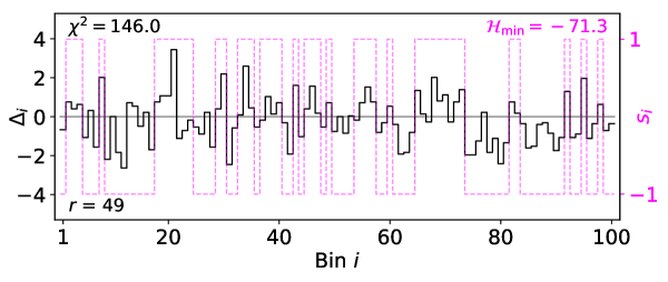
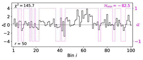
Figure 1: Results from two representative pseudo-experiments with similar $\chi^{2}$ values: without signal (top) and with signal (bottom). The black solid histogram shows the deviations (1), while the magenta dotted histogram depicts the corresponding spin configuration which minimizes the Hamiltonian (2).

3 Results with one-dimensional data

In order to demonstrate the appropriateness of the Hamiltonian (2), we first consider the following one-dimensional toy example illustrated in Fig. 1. We take 100 equal-size bins which are populated with data sampled from a background distribution, which we take to be uniform, with an expected total number of 50000 events; and a signal distribution, which we take to be a normal distribution centered on the 60th bin with a standard deviation of 5 bin widths, and an expected total number of 500 signal events. In order to test the power of the ${\cal H}_{min}$ test, we generate 10000 pseudo-experiments under the background hypothesis (top panel in Fig. 1) and background plus signal hypothesis (bottom panel). For each pseudo-experiment, we first compute the resulting deviations (1) shown with the black solid histogram and construct the Ising Hamiltonian (2). Then, using the method of simulated annealing [53], we find the spin configuration $\{s_{i}\}$ (shown with the magenta dotted histogram) which minimizes the Hamiltonian and gives the ground state energy (3). Comparing the two types of histograms in Fig. 1, we observe that the spins in the ground state indeed tend to align themselves in the regions where the deviations are strong and/or correlated, which is precisely what the Hamiltonian (2) was designed to accomplish.

The two panels in Fig. 1 depict two pseudo-experiments whose $\chi^{2}$ values are rather similar, 146 and 145.7, respectively. Therefore, as far as the $\chi^{2}$ test statistic is concerned, these two sets of data appear very similar, even though the excess around 60 is rather evident to the trained eye. On the other hand, these two experiments produce rather different values for the ${\mathcal{H}}_{min}$ test statistic: $-71.3$ for the pure background case and $-82.5$ for the background plus signal case. This implies that the ${\mathcal{H}}_{min}$ test statistic can better identify such signals in the data. A more thorough comparison of the discriminating powers of the $\chi^{2}$ and ${\mathcal{H}}_{min}$ test statistics is presented in Figs. 3 and 3. The left and right panels in Fig. 3 show the unit-normalized distributions of the $\chi^{2}$ and ${\mathcal{H}}_{min}$ test statistics, respectively, for large sets of pseudo-experiments under the background hypothesis (black solid lines) and the background plus signal hypothesis (black dashed lines). In order to accumulate enough statistics for the plots, in the left (right) panel of Fig. 3, we use data from 10000 (1000) pseudo-experiments. In addition, in order to have the histograms similarly ordered from left to right on the two panels, in the right panel we chose to plot $-{\mathcal{H}}_{min}$ instead of ${\mathcal{H}}_{min}$. We observe that in the case of the ${\mathcal{H}}_{min}$ test statistics (right panel) the distribution with signal is further separated from the corresponding distribution for the null hypothesis, thus implying higher sensitivity.

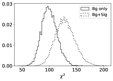
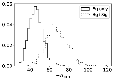
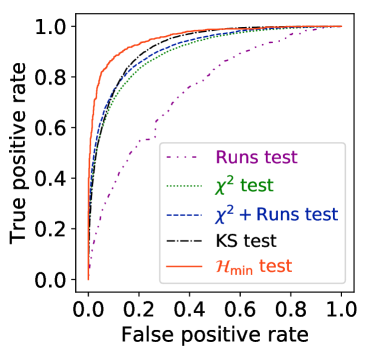
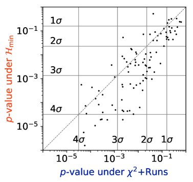
Figure 2: Normalized distributions of the $\chi^{2}$ (left panel) and the $-{\mathcal{H}}_{min}$ (right panel) test statistics for the respective set of pseudo-experiments under the null (pure background) hypothesis (black solid lines) and the background plus signal hypothesis (black dashed lines).

Figure 3: Left: ROC curves for: our ${\mathcal{H}}_{min}$ test statistic (orange solid line), the Wald–Wolfowitz runs test (purple dot-dot-dashed), $\chi^{2}$-test (green dotted), combined $\chi^{2}$ plus runs test (blue dashed), and the Kolmogorov-Smirnov test (black dot-dashed). Right: Scatter plot of the estimated $p$-values for 100 representative pseudo-experiments produced under the signal hypothesis, under the combined $\chi^{2}$ plus runs test ($x$-axis) and the ${\mathcal{H}}_{min}$ test statistic ($y$-axis). The grid lines mark the $p$-values corresponding to a 1$\sigma$, 2$\sigma$, 3$\sigma$ and 4$\sigma$ effect.

In the left panel of Fig. 3 we compare the sensitivity of our new test statistic to several standard goodness-of-fit tests in terms of the corresponding receiver operating characteristic (ROC) curves [54]. Results are shown for the new ${\mathcal{H}}_{min}$ test statistic (orange solid line), the Wald–Wolfowitz runs test (purple dot-dot-dashed), $\chi^{2}$-test (green dotted), combined $\chi^{2}$ plus runs test (blue dashed), and the Kolmogorov–Smirnov test [48] (black dot-dashed). It is clear that the new ${\mathcal{H}}_{min}$ test statistic outperforms all others, especially in the low false positive rate region which is relevant for discovery. The implications for discovery are further illustrated in the right panel of Fig. 3, which shows a scatter plot of estimated $p$-values under the combined $\chi^{2}$ plus runs test ($x$-axis) and the ${\mathcal{H}}_{min}$ test statistic ($y$-axis), for 100 representative pseudo-experiments produced under the signal plus background hypothesis. We observe that for the large majority of the pseudo-experiments, namely, those below the $45^{\circ}$ dashed line, ${\mathcal{H}}_{min}$ gives a higher significance of discovery.

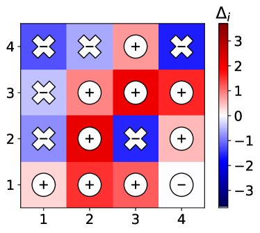
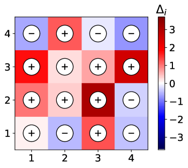
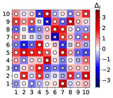
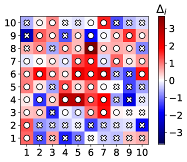
Figure 4: Results from two representative pseudo-experiments with similar $\chi^{2}$ values for the $4\times 4$ two-dimensional exercise: without signal (left) and with signal (right), with the signal $2\times 2$ block located in the middle of the $4\times 4$ grid. Warm (cool) colors and plusses (minuses) indicate upward (downward) fluctuations (1). Circles (crosses) indicate spin orientations $s_{i}=+1$ ($s_{i}=-1$) in the ${\mathcal{H}}_{min}$ spin configuration.

Figure 5: The same as Fig. 5, but for the $10\times 10$ exercise. The signal in the right panel is injected as an uncorrelated bivariate normal distribution with equal standard deviations of $1.5$ bin widths. Both pseudo-experiments have $\chi^{2}=129$.

4 Results with two-dimensional data

Unlike existing tests sensitive to spatial correlations, our technique can be readily generalized to multi-dimensional data. This is illustrated in Figs. 5 – 8, where for simplicity we limit ourselves to two dimensions and consider data arranged in an $n\times n$ grid of $N=n^{2}$ bins. In Fig. 5 we take $n$ to be relatively low, $n=4$. This allows us to find the minimum energy ${\mathcal{H}}_{min}$ by brute force, i.e., by inspecting each of the $2^{N}=2^{16}$ spin configurations and comparing the corresponding energies. Then in Fig. 5 we consider a larger grid with $n=10$, for which the brute force method is unfeasible, and in order to find ${\mathcal{H}}_{min}$ we resort back to the method of simulated annealing used in the earlier one-dimensional example. In the $4\times 4$ case of Fig. 5, the $\Delta_{i}$ values for the background are sampled directly from the standard normal distribution, and the signal is then modelled as a constant $1.5\sigma$ additional contribution to each bin in a $2\times 2$ block of the $4\times 4$ grid. The color code used in Fig. 5 reflects the resulting $\Delta_{i}$ values for the two pseudo-experiments — upward (downward) fluctuations $\Delta_{i}$ are represented with warm (cool) colors and marked with plus (minus) signs. In the $10\times 10$ case of Fig. 5, the data values $o_{i}$ for the background are sampled from a Poisson distribution with $e_{i}=500$ in each bin. An uncorrelated bivariate normal signal of 600 total expected events is then injected at the location of the $(6,6)$ bin. The resulting deviations $\Delta_{i}$ are then computed and shown for two representative pseudo-experiments in Fig. 5, using the same color-code as in Fig. 5. Note that the index $i$ in eqs. (1-4) is now two-dimensional and identifies the horizontal and vertical location of the respective bin; two bins are considered nearest neighbors only if they share an edge.

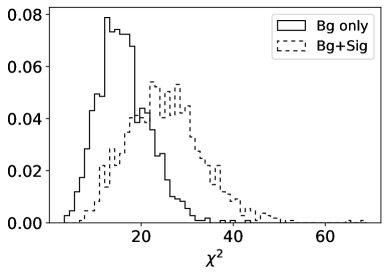
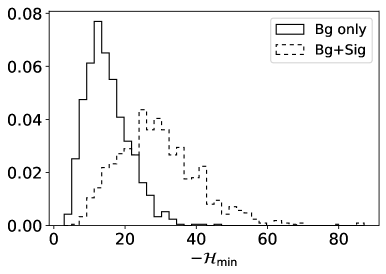
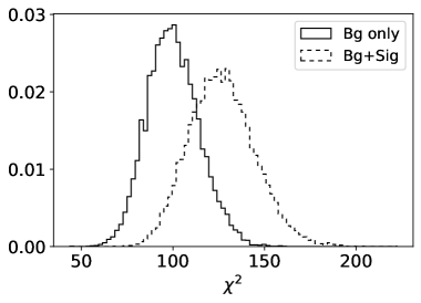
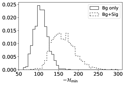
Figure 6: The same as Fig. 3, but for the $4\times 4$ two-dimensional exercise illustrated in Fig. 5.

Figure 7: The same as Fig. 7, but for the $10\times 10$ two-dimensional exercise illustrated in Fig. 5.

In complete analogy to Fig. 3, in Figs. 7 and 7 we show the respective distributions of the $\chi^{2}$ and $-{\mathcal{H}}_{min}$ test statistics for each of the two-dimensional examples considered in this section. We notice that, just like in the case of the one-dimensional exercise depicted in Fig. 3, the ${\mathcal{H}}_{min}$ test statistic offers better separation of signal and background. For example, in Fig. 7 the overlap area between the two distributions is 51.3% in the case of the $\chi^{2}$ test statistic, but only 41.4% in the case of ${\mathcal{H}}_{min}$. The improvement is even better in the case of the $10\times 10$ grid — in Fig. 7, the overlap area is 40.7% for the $\chi^{2}$ test statistic and is reduced to only 20.1% in the case of ${\mathcal{H}}_{min}$.

Motivated by the usefulness of the runs test in the one-dimensional example of Figs. 1 and 3, we can attempt to generalize it to the two-dimensional data of Figs. 5 and 5. For example, we can count the number of connected “regions” of only positive or only negative deviations $\Delta_{i}$, defined so that nearest neighbors with the same $\text{sgn}(\Delta_{i})$ necessarily belong to the same region. In that case, each of the two pseudo-experiments in Fig. 5 leads to 5 regions, as can be easily seen by inspecting the plusses and minuses shown in the bins. However, the so defined “regions” test statistic is not very powerful, as can be seen from the respective ROC curves in Fig. 8 — in fact, combining the “regions” test with the $\chi^{2}$ statistic generally makes things worse than using $\chi^{2}$ alone.

This is where the new test statistic ${\mathcal{H}}_{min}$ comes to the rescue. Figs. 5 and 5 depict the spin configurations in the respective ground states: circles indicate spin orientation $s_{i}=+1$ while crosses correspond to $s_{i}=-1$. The corresponding ROC curves in Fig. 8 (orange solid lines) demonstrate the superior performance of the ${\mathcal{H}}_{min}$ test statistic for these two-dimensional examples as well.

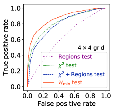
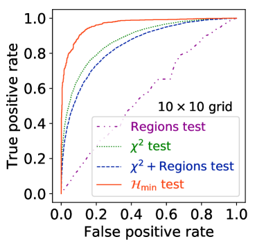
Figure 8: ROC curves for the two-dimensional exercises with $4\times 4$ data as in Fig. 5 (left) and $10\times 10$ data as in Fig. 5 (right).

5 Conclusions and outlook

In this paper we proposed a new goodness-of-fit test statistic, ${\mathcal{H}}_{min}$, to identify deviations from an expectation, without assuming any alternative hypothesis to account for the deviations. Our test statistic exploits in a novel, model-independent way, the spatial correlations in the observed fluctuations of binned data relative to a theoretical prediction. Our method for anomaly detection greatly reduces the look-elsewhere effect by exploiting the typical differences between the properties of statistical noise and real new physics effects. With several toy examples, we demonstrated that the ${\mathcal{H}}_{min}$ test performs better than some commonly used goodness-of-fit tests. Once a signal is detected, the spin configuration in the ground state can be inspected to identify atypically large domains of aligned spins which can then be used to interpret the origin of the anomaly detected by our statistic.

When an experiment calls for an analysis with a large number of bins (i.e., lattice spin sites) $N$, the exact computation of ${\mathcal{H}}_{min}$ becomes intractable and must be handled via a suitable approximate method. A promising approach to tackle large $N$ cases is offered by current and future AQO implementations on quantum computers [55, 56, 57]. In the meantime, an acceptable alternative is to apply approximate stochastic optimization methods like simulated annealing, which was used in our analysis.

In this paper, we assumed that the theoretical expectation $\{e_{i}\}$ is known exactly. However, in realistic situations, e.g., in the presence of systematic uncertainties, it may depend on various nuisance parameters $\vec{\theta}$, in which case the test statistic can be modified as

$$\max_{\vec{\theta}}\left\{{\mathcal{H}}_{min}\left(\vec{\theta}\right)\right\},$$ (7)

which will be discussed in a longer paper [52]. We are also in the process of exploring a larger class of Hamiltonians and their relevance to various combinatorial optimization problems, both inside and outside particle physics. We believe this work is only scratching the surface of a very interesting new direction of interdisciplinary research bridging condensed matter physics (Ising models), quantum information science, computational geometry, statistics and high energy physics.

6 Acknowledgements

The authors would like to thank D. Acosta, I. Furic, S. Hoffman, P. Ramond, J. Taylor, W. Xue, and especially S. Mrenna for useful discussions. The work of KM and PS is supported in part by the US Department of Energy under Grant No. DE-SC0010296. The work of PS is supported by the University of Florida CLAS Dissertation Fellowship funded by the Charles Vincent and Heidi Cole McLaughlin Endowment. PS is grateful to the LHC Physics Center at Fermilab for hospitality and financial support as part of the Guests and Visitors Program in the summer of 2019.

References

- [1] G. Aad et al. [ATLAS Collaboration], “Observation of a new particle in the search for the Standard Model Higgs boson with the ATLAS detector at the LHC,” Phys. Lett. B 716, 1 (2012) doi:10.1016/j.physletb.2012.08.020 [arXiv:1207.7214 [hep-ex]].
- [2] S. Chatrchyan et al. [CMS Collaboration], “Observation of a New Boson at a Mass of 125 GeV with the CMS Experiment at the LHC,” Phys. Lett. B 716, 30 (2012) doi:10.1016/j.physletb.2012.08.021 [arXiv:1207.7235 [hep-ex]].
- [3] B. Abbott et al. [D0 Collaboration], “Search for new physics in data at DØ using Sherlock: A quasi model independent search strategy for new physics,” Phys. Rev. D 62, 092004 (2000) doi:10.1103/PhysRevD.62.092004 [hep-ex/0006011].
- [4] V. M. Abazov et al. [D0 Collaboration], “A Quasi model independent search for new physics at large transverse momentum,” Phys. Rev. D 64, 012004 (2001) doi:10.1103/PhysRevD.64.012004 [hep-ex/0011067].
- [5] B. Abbott et al. [D0 Collaboration], “A quasi-model-independent search for new high physics at DØ,” Phys. Rev. Lett. 86, 3712 (2001) doi:10.1103/PhysRevLett.86.3712 [hep-ex/0011071].
- [6] A. Aktas et al. [H1 Collaboration], “A General search for new phenomena in ep scattering at HERA,” Phys. Lett. B 602, 14 (2004) doi:10.1016/j.physletb.2004.09.057 [hep-ex/0408044].
- [7] M. Wessels [H1 Collaboration], “A General Search for New Phenomena in e-p Scattering at HERA,” arXiv:0705.3721 [hep-ex].
- [8] T. Aaltonen et al. [CDF Collaboration], “Model-Independent and Quasi-Model-Independent Search for New Physics at CDF,” Phys. Rev. D 78, 012002 (2008) doi:10.1103/PhysRevD.78.012002 [arXiv:0712.1311 [hep-ex]].
- [9] T. Aaltonen et al. [CDF Collaboration], “Model-Independent Global Search for New High-p(T) Physics at CDF,” doi:10.2172/922303 arXiv:0712.2534 [hep-ex].
- [10] T. Aaltonen et al. [CDF Collaboration], “Global Search for New Physics with 2.0 fb-1 at CDF,” Phys. Rev. D 79, 011101 (2009) doi:10.1103/PhysRevD.79.011101 [arXiv:0809.3781 [hep-ex]].
- [11] F. D. Aaron et al. [H1 Collaboration], “A General Search for New Phenomena at HERA,” Phys. Lett. B 674, 257 (2009) doi:10.1016/j.physletb.2009.03.034 [arXiv:0901.0507 [hep-ex]].
- [12] V. M. Abazov et al. [D0 Collaboration], “Model independent search for new phenomena in collisions at TeV,” Phys. Rev. D 85, 092015 (2012) doi:10.1103/PhysRevD.85.092015 [arXiv:1108.5362 [hep-ex]].
- [13] [CMS Collaboration], “MUSIC – An Automated Scan for Deviations between Data and Monte Carlo Simulation,” CMS-PAS-EXO-08-005.
- [14] D. Duchardt, “MUSiC: A Model Unspecific Search for New Physics Based on CMS Data,” doi:10.18154/RWTH-2017-07986
- [15] M. Aaboud et al. [ATLAS Collaboration], “A strategy for a general search for new phenomena using data-derived signal regions and its application within the ATLAS experiment,” Eur. Phys. J. C 79, no. 2, 120 (2019) doi:10.1140/epjc/s10052-019-6540-y [arXiv:1807.07447 [hep-ex]].
- [16] D. Debnath, J. S. Gainer, D. Kim and K. T. Matchev, “Edge Detecting New Physics the Voronoi Way,” EPL 114, no. 4, 41001 (2016) doi:10.1209/0295-5075/114/41001 [arXiv:1506.04141 [hep-ph]].
- [17] D. Debnath, J. S. Gainer, C. Kilic, D. Kim, K. T. Matchev and Y. P. Yang, “Identifying Phase Space Boundaries with Voronoi Tessellations,” Eur. Phys. J. C 76, no. 11, 645 (2016) doi:10.1140/epjc/s10052-016-4431-z [arXiv:1606.02721 [hep-ph]].
- [18] E. M. Metodiev, B. Nachman and J. Thaler, “Classification without labels: Learning from mixed samples in high energy physics,” JHEP 1710, 174 (2017) doi:10.1007/JHEP10(2017)174 [arXiv:1708.02949 [hep-ph]].
- [19] J. A. Aguilar-Saavedra, J. H. Collins and R. K. Mishra, “A generic anti-QCD jet tagger,” JHEP 1711, 163 (2017) doi:10.1007/JHEP11(2017)163 [arXiv:1709.01087 [hep-ph]].
- [20] J. H. Collins, K. Howe and B. Nachman, “Anomaly Detection for Resonant New Physics with Machine Learning,” Phys. Rev. Lett. 121, no. 24, 241803 (2018) doi:10.1103/PhysRevLett.121.241803 [arXiv:1805.02664 [hep-ph]].
- [21] A. De Simone and T. Jacques, “Guiding New Physics Searches with Unsupervised Learning,” Eur. Phys. J. C 79, no. 4, 289 (2019) doi:10.1140/epjc/s10052-019-6787-3 [arXiv:1807.06038 [hep-ph]].
- [22] J. Hajer, Y. Y. Li, T. Liu and H. Wang, “Novelty Detection Meets Collider Physics,” arXiv:1807.10261 [hep-ph].
- [23] T. Heimel, G. Kasieczka, T. Plehn and J. M. Thompson, “QCD or What?,” SciPost Phys. 6, no. 3, 030 (2019) doi:10.21468/SciPostPhys.6.3.030 [arXiv:1808.08979 [hep-ph]].
- [24] M. Farina, Y. Nakai and D. Shih, “Searching for New Physics with Deep Autoencoders,” arXiv:1808.08992 [hep-ph].
- [25] A. Casa and G. Menardi, “Nonparametric semisupervised classification for signal detection in high energy physics,” arXiv:1809.02977 [stat.AP].
- [26] O. Cerri, T. Q. Nguyen, M. Pierini, M. Spiropulu and J. R. Vlimant, “Variational Autoencoders for New Physics Mining at the Large Hadron Collider,” JHEP 1905, 036 (2019) doi:10.1007/JHEP05(2019)036 [arXiv:1811.10276 [hep-ex]].
- [27] J. H. Collins, K. Howe and B. Nachman, “Extending the search for new resonances with machine learning,” Phys. Rev. D 99, no. 1, 014038 (2019) doi:10.1103/PhysRevD.99.014038 [arXiv:1902.02634 [hep-ph]].
- [28] T. S. Roy and A. H. Vijay, “A robust anomaly finder based on autoencoder,” arXiv:1903.02032 [hep-ph].
- [29] B. M. Dillon, D. A. Faroughy and J. F. Kamenik, “Uncovering latent jet substructure,” Phys. Rev. D 100, no. 5, 056002 (2019) doi:10.1103/PhysRevD.100.056002 [arXiv:1904.04200 [hep-ph]].
- [30] A. Blance, M. Spannowsky and P. Waite, “Adversarially-trained autoencoders for robust unsupervised new physics searches,” JHEP 1910, 047 (2019) doi:10.1007/JHEP10(2019)047 [arXiv:1905.10384 [hep-ph]].
- [31] A. Mullin, H. Pacey, M. Parker, M. White and S. Williams, “Does SUSY have friends? A new approach for LHC event analysis,” arXiv:1912.10625 [hep-ph].
- [32] B. Nachman and D. Shih, “Anomaly Detection with Density Estimation,” arXiv:2001.04990 [hep-ph].
- [33] O. Behnke, K. Kröninger, T. Schörner-Sadenius and G. Schott (Editors), “Data analysis in high energy physics : A practical guide to statistical methods,” Wiley-VCH, 2013.
- [34] R. T. D’Agnolo and A. Wulzer, “Learning New Physics from a Machine,” Phys. Rev. D 99, no. 1, 015014 (2019) doi:10.1103/PhysRevD.99.015014 [arXiv:1806.02350 [hep-ph]].
- [35] R. T. D’Agnolo, G. Grosso, M. Pierini, A. Wulzer and M. Zanetti, “Learning Multivariate New Physics,” arXiv:1912.12155 [hep-ph].
- [36] Y. F. Contoyiannis, S. Potirakis and F. K. Diakonos, “Wavelet based detection of scaling behaviour in noisy experimental data,” arXiv:1905.01153 [physics.data-an].
- [37] B. G. Lillard, T. Plehn, A. Romero and T. M. P. Tait, “Multi-scale Mining of Kinematic Distributions with Wavelets,” arXiv:1906.10890 [hep-ph].
- [38] H. Beauchesne and Y. Kats, “Searching for periodic signals in kinematic distributions using continuous wavelet transforms,” arXiv:1907.03676 [hep-ph].
- [39] R. J. Baxter, “Exactly Solvable Models in Statistical Mechanics," Dover Publications, Mineola NY, 2007.
- [40] S. Kirkpatrick, C. D. Gelatt and M. P. Vecchi, “Optimization by Simulated Annealing,” Science 220, 671 (1983). doi:10.1126/science.220.4598.671
- [41] E. Farhi, J. Goldstone, S. Gutmann and M. Sipser, “Quantum Computation by Adiabatic Evolution," arXiv:quant-ph/0001106
- [42] E. Farhi, J. Goldstone, S. Gutmann, J. Lapan, A. Lundgren and D. Preda, “A Quantum Adiabatic Evolution Algorithm Applied to Random Instances of an NP-Complete Problem," Science 292 472 (2001) [quant-ph/0104129].
- [43] W. van Dam, M. Mosca and U. V. Vazirani, “How powerful is adiabatic quantum computation?", Proceedings 2001 IEEE International Conference on Cluster Computing, 279-287 (2001).
- [44] A. Das and B. K. Chakrabarti, “Colloquium: Quantum annealing and analog quantum computation,” Rev. Mod. Phys. 80, 1061 (2008) doi:10.1103/RevModPhys.80.1061 [arXiv:0801.2193 [quant-ph]].
- [45] A. Lucas, “Ising formulations of many NP problems," Frontiers in Physics 2 (2014) [arXiv:1302.5843 [cond-mat.stat-mech]].
- [46] A. Mott, J. Job, J. R. Vlimant, D. Lidar and M. Spiropulu, “Solving a Higgs optimization problem with quantum annealing for machine learning,” Nature 550, no. 7676, 375 (2017), doi:10.1038/nature24047.
- [47] K. Cormier, R. Di Sipio and P. Wittek, “Unfolding measurement distributions via quantum annealing,” JHEP 1911, 128 (2019) doi:10.1007/JHEP11(2019)128 [arXiv:1908.08519 [physics.data-an]].
- [48] G. Schott, “Hypothesis testing", chapter 3 in Ref. [33].
- [49] A. Wald and J. Wolfowitz, “On a test whether two samples are from the same population," Ann. Math. Stat., 11 (1940) 147.
- [50] R. A. Fisher, “Statistical Methods for Research Workers,” Oliver and Boyd, Edinburgh, (1925).
- [51] R. A. Fisher, “Questions and answers #14,” The American Statistician 2 no 5, 30 (1948), doi:10.2307/2681650.
- [52] K. T. Matchev, P. Shyamsundar and J. Smolinsky, “Further exploration of Ising models for goodness-of-fit tests in new physics searches," in preparation.
- [53] H. Guo, M. Zuckermann, R. Harris and M. Grant, “A Fast Algorithm for Simulated Annealing," Physica Scripta 1991 (1991) 40.
- [54] T. Fawcett, “An introduction to ROC analysis,” Pattern Recognition Letters, 27, no. 8, 861874 (2006).
- [55] P. I. Bunyk, E. M. Hoskinson, M. W. Johnson, E. Tolkacheva, F. Altomare, A. J. Berkley, R. Harris, J. P. Hilton, T. Lanting, A. J. Przybysz and J. Whittaker, “Architectural considerations in the design of a superconducting quantum annealing processor,” IEEE Transactions on Applied Superconductivity 24, 1 (Aug. 2014).
- [56] T. Albash and D. A. Lidar, “Demonstration of a Scaling Advantage for a Quantum Annealer over Simulated Annealing,” Phys. Rev. X 8, no. 3, 031016 (2018) doi:10.1103/PhysRevX.8.031016 [arXiv:1705.07452 [quant-ph]].
- [57] N. Dattani, S. Szalay and N. Chancellor, “Pegasus: The second connectivity graph for large-scale quantum annealing hardware," arXiv:1901.07636 [quant-ph].
- [58] S. Boixo, T. F. Rønnow, S. V. Isakov, Z. Wang, D. Wecker, D. A. Lidar, J. M. Martinis, M. Troyer, “Quantum annealing with more than one hundred qubits,” Nature Phys. 10, 218 (2014) [arXiv:1304.4595 [quant-ph]].
- [59] T. F. Rønnow, Z. Wang, J. Job, S. Boixo, S. V. Isakov, D. Wecker, J. M. Martinis, D. A. Lidar, M. Troyer, “Defining and detecting quantum speedup,” Science 345, 420 (2014) [arXiv:1401.2910 [quant-ph]].
- [60] O. Parekh, J. Wendt, L. Shulenburger, A. Landahl, J. Moussa, J. Aidun, “Benchmarking Adiabatic Quantum Optimization for Complex Network Analysis," arXiv:1604.00319 [quant-ph].