Magnetic dipole excitations based on the relativistic nuclear energy density functional

Abstract

Magnetic dipole (M1) excitations build not only a fundamental mode of nucleonic transitions, but they are also relevant for nuclear astrophysics applications. We have established a theory framework for description of M1 transitions based on the relativistic nuclear energy density functional. For this purpose the relativistic quasiparticle random phase approximation (RQRPA) is established using density dependent point coupling interaction DD-PC1, supplemented with the isovector-pseudovector interaction channel in order to study unnatural parity transitions. The introduced framework has been validated using the M1 sum rule for core-plus-two-nucleon systems, and employed in studies of the spin, orbital, isoscalar and isovector M1 transition strengths, that relate to the electromagnetic probe, in magic nuclei ⁴⁸Ca and ²⁰⁸Pb, and open shell nuclei ⁴²Ca and ⁵⁰Ti. In these systems, the isovector spin-flip M1 transition is dominant, mainly between one or two spin-orbit partner states. It is shown that pairing correlations have a significant impact on the centroid energy and major peak position of the M1 mode. The M1 excitations could provide an additional constraint to improve nuclear energy density functionals in the future studies.

I Introduction

Electromagnetic excitations in finite nuclei represent one of the most important probes of relevance in nuclear structure and dynamics, as well as in nuclear astrophysics. In particular, various aspects of magnetic dipole (M1) mode have been considered both in experimental and theoretical studies Richter (1985, 1995); Heyde et al. (2010); Kneissl et al. (1996); Pietralla et al. (2008); Shizuma et al. (2008); Goriely (2015); Goriely et al. (2016) due to its relevance for diverse nuclear properties associated e.g., to unnatural-parity states, spin-orbit splittings and tensor force effects. Specifically, M1 spin-flip excitations are analog of Gamow-Teller (GT) transitions, meaning that, at the operator level, the dominant M1 isovector component is the synonym to the zeroth component of GT transitions, and can serve as probe for calculations of inelastic neutrino-nucleus cross section Langanke et al. (2004); Langanke and Martínez-Pinedo (2003). This process is hard to measure but it is essential in supernova physics, as well as in the r-process nucleosynthesis calculations Langanke et al. (2008); Loens et al. (2012); Goriely (2015); Goriely et al. (2016). The isovector spin-flip M1 response is also relevant for applications related to the design of nuclear reactors Chadwick and et. al. (2011), for the understanding of single-particle properties, spin-orbit interaction, and shell closures from stable nuclei toward limits of stability Otsuka et al. (2005, 2010); Vesely et al. (2009); Nesterenko et al. (2010); Tselyaev et al. (2019), as well as for the resolving the problem of quenching of the spin-isopin response in nuclei that is necessary for reliable description of double beta decay matrix elements Vergados et al. (2012). In deformed nuclei, another type of M1 excitations has been extensively studied, known as scissors mode, where the orbital part of M1 operator plays a dominant role in a way that protons and neutrons oscillate with opposite phase around the core Arteaga and Ring (2008); Ebran et al. (2011); Heyde et al. (2010); Richter (1990); Otsuka (1990); Bohle et al. (1984a, b); Schwengner et al. (2017); Balbutsev et al. (2018); Repko et al. (2019).

In any nuclei undergoing experimental investigation, there are simultaneously present $E\lambda$ and $M\lambda$ multipole excitations, where the electric dipole (E1) and electric quadrupole (E2) responses Oishi and Paar (2019); Dang and Hung (2013); Yoshida (2009); Terasaki and Engel (2011); Ebata et al. (2014); Stetcu et al. (2011) dominate over M1 response Tamii et al. (2007); Fujita et al. (2011a); Birkhan et al. (2016); Laszewski et al. (1988, 1985); Laszewski and Axel (1979); Laszewski et al. (1977); Chrien and Kane (1979); Raman et al. (1977). Thus, it is a rather challenging task to measure M1-related observables in a whole energy range. Even for the nuclides accessible by experiments, their full information on the M1 response has not been complete.

The M1 transitions have been studied in various theoretical approaches. Various aspects of the M1 mode have been investigated in the shell model Richter (1990); Otsuka et al. (2010); Loens et al. (2012); Sieja (2018); Otsuka et al. (2005); Langanke et al. (2004); Maripuu (1969), including, e.g., scissors and unique-parity modes Richter (1990), tensor-force effect Otsuka et al. (2005), low-energy enhancement of radiation Sieja (2018), and the analogy with neutrino-nucleus scattering Langanke et al. (2004); Loens et al. (2012). The M1 energy-weighted sum rule has been discussed from a perspective of the spin-orbit energy Kurath (1963). The Landau-Migdal interaction has been one of the relevant topics in studies of M1 excitations Migli et al. (1991); Kamerdzhiev et al. (1993). In order to reproduce a large fragmentation of the experimental M1 strength, the importance of including complex couplings going beyond the RPA level has also been addressed Migli et al. (1991); Kamerdzhiev et al. (1993); Moraghe et al. (1994); Marcucci et al. (2008); Schwengner et al. (2017).

Recently, the M1 excitation has been investigated in the framework based on the Skryme functionals Vesely et al. (2009); Nesterenko et al. (2010); Tselyaev et al. (2019), also extended to include tensor effects Cao et al. (2009). It has been shown that the results for the spin-flip resonance obtained by using different parameterizations do not appear as convincing interpretation of the experimental results. Additional effects have been explored in order to resolve this issue, e.g., the isovector-M1 response versus isospin-mixed responses, and the role of tensor and vector spin-orbit interactions Vesely et al. (2009); Nesterenko et al. (2010). In recent analysis in Ref. Speth et al. (2020), based on the Skyrme functionals, it has been shown that while modern Skyrme parameterizations successfully reproduce electric excitations, there are difficulties to describe magnetic transitions. In addition, some Skyrme sets result in the ambiguity that, by the same parameterization, the model cannot simultaneously describe one-peak and two-peak data for closed and open shell nuclei Vesely et al. (2009). Thus, further developments of the Skyrme functional in the spin channel are called for Speth et al. (2020). Simultaneously, it is essential to explore the M1 response from different theoretical approaches to achieve a complete understanding of their properties, as well as to assess the respective systematic uncertainties.

The aim of this work is to describe the properties of M1 excitations from a different perspective, by implementing a novel theory framework derived from the relativistic nuclear energy density functional. This framework has been in the past successfully employed in description of a variety of nuclear properties and astrophysically relevant processes Vretenar et al. (2005); Nikšić et al. (2005); Paar et al. (2007, 2008); Niu et al. (2009); Khan et al. (2011); Paar et al. (2014); Roca-Maza et al. (2015); Nikšić et al. (2015); Paar et al. (2015); Vale et al. (2016); Roca-Maza and Paar (2018); Nikšić et al. (2014); Yüksel et al. (2019). In open shell nuclei, the pairing correlations make unnegligible contributions to the properties of M1 transitions Pai et al. (2016); Oishi and Paar (2019), thus they are also included in model calculations.

The paper is organized as follows. In Sec. II the overview of the formalism of the relativistic quasiparticle random phase approximation (QRPA) for magnetic transitions based on the relativistic point-coupling interaction is given. Section II.3 is devoted to display the benchmark result of our relativistic QRPA scheme in comparison with the sum rule in Ref. Oishi and Paar (2019). The results of model calculations and comparison with the experimental studies are presented in Secs. III.1 and III.2, while the pairing effects are considered in Sec. III.3. A summary of the present work is given in Sec. IV.

II Formalism

We study M1 excitations based on particle-hole ($1p\mathchar 45\relax 1h$) (or in open shell nuclei two-quasiparticle) transitions from $0^{+}$ ground state (GS) to $1^{+}$ excited states of even-even nuclei within the formalism of a relativistic nuclear energy density functional (RNEDF), assuming the spherical symmetry Nikšić et al. (2014). More details about the RNEDF and its implementations are given in Refs. Nikšić et al. (2014, 2008). In this work, the nuclear ground state has been calculated by employing the self-consistent relativistic Hartree-Bogoliubov (RHB) model Nikšić et al. (2014), where the mean field is derived for the relativistic point-coupling interaction with density-dependent couplings. Many effects that go beyond the mean-field level are not explicitely included in the RHB model, e.g., Fock terms, vacuum polarization effects and the short-range Brueckner-type correlations. Since the parameters of the RNEDF are adjusted to the experimental data which contain all these and other effects, it means that effects beyond the mean-field level are implicitly included in the RHB approach by adjusting the model parameters to reproduce a selected empirical data set Vretenar et al. (2005). The no-sea approximation is also employed for relativistic mean-field calculations Vretenar et al. (2005).

Here we briefly present the formalism of the relativistic point coupling interaction starting from the Lagrangian density,

$$\mathcal{L} =\bar{\Psi}_{N}(i\gamma^{\mu}\partial_{\mu}-m_{0N})\Psi_{N}$$ (1)

$$-\frac{1}{2}\alpha_{S}(\rho)(\bar{\Psi}_{N}{\Psi}_{N})(\bar{\Psi}_{N}{\Psi}_{N})$$

$$-\frac{1}{2}\alpha_{V}(\rho)(\bar{\Psi}_{N}\gamma^{\nu}{\Psi}_{N})(\bar{\Psi}_{N}\gamma_{\nu}{\Psi}_{N})$$

$$-\frac{1}{2}\alpha_{TV}(\rho)(\bar{\Psi}_{N}\vec{\tau}\gamma^{\nu}{\Psi}_{N})\cdot(\bar{\Psi}_{N}\vec{\tau}\gamma_{\nu}{\Psi}_{N})$$

$$-\frac{1}{2}\delta_{S}(\partial_{\nu}\bar{\Psi}_{N}{\Psi}_{N})(\partial^{\nu}\bar{\Psi}_{N}{\Psi}_{N})$$

$$-e\bar{\Psi}_{N}(\gamma^{\nu}A_{\nu}(\vec{x}))\frac{1-\hat{\tau_{3}}}{2}\Psi_{N}.$$

The first term corresponds to the free nucleon field of Dirac type, while the point coupling interaction terms include isoscalar-scalar ($J^{\pi}=0^{+}$), isoscalar-vector ($J^{\pi}=1^{-}$), isovector-vector ($J^{\pi}=1^{-}$) channels (where $J$ denotes the respective quantum number for the angular momentum and $\pi$ for the parity), coupling of protons to the electromagnetic field, and the derivative term accounting for the leading effects of finite-range interactions necessary for a quantitative description of nuclear density distribution and radii.

The density dependent couplings in each channel, $\alpha_{S}(\rho)$ (isoscalar-scalar), $\alpha_{V}(\rho)$ (isoscalar-vector), and $\alpha_{TV}(\rho)$ (isovector-vector) are modeled by well-behaved functional Nikšić et al. (2014),

$$\alpha_{i}(\rho)=a_{i}+(b_{i}+c_{i}x)e^{-d_{i}x},$$ (2)

where $x=\frac{\rho}{\rho_{sat.}}$ and $\rho_{sat.}$ denotes nucleon density at saturation point for the case of symmetric nuclear matter. The respective parameters for each channel $i=S,V,TV$ are denoted as $a_{i}$, $b_{i}$, $c_{i}$ and $s_{i}$, while $\delta_{S}$ denotes the strength of isoscalar-scalar derivative term. In this work the DD-PC1 parameterization is used in model calculations Nikšić et al. (2014). The RHB model employed in this study includes pairing correlations described by the pairing part of the phenomenological Gogny interaction Vretenar et al. (2005),

$$V^{pp}(1,2)=\sum_{i=1,2} e^{[(\bm{r}_{1}-\bm{r}_{2})/\mu_{i}]^{2}}\left(W_{i}+B_{i}\hat{P}^{\sigma}\right.$$ (3)

$$\left.-H_{i}\hat{P}^{\tau}-M_{i}\hat{P}^{\sigma}\hat{P}^{\tau}\right),$$

where $\hat{P}^{\sigma}$ and $\hat{P}^{\tau}$ indicate the exchanges of the spin and isospin, respectively. The parameters $\mu_{i}$, $W_{i}$, $B_{i}$, $H_{i}$ and $M_{i}$ ($i=1,2$) are given by the D1S set as in Ref. Berger et al. (1991). We confirmed that, combined with the DD-PC1 functional for the mean-field part, this parameterization sufficiently reproduces the empirical pairing gaps of open-shell systems in this study.

For the M1 excitations of nuclei, we utilize the relativistic quasiparticle random phase approximation (RQRPA) Paar et al. (2003), that is in this work developed for the implementation of the relativistic point-coupling interaction, extended to describe the unnatural-parity transitions of M1 type. In the limit of small amplitude oscillations, the RQRPA matrix equations read,

$$\begin{pmatrix}A^{J}&B^{J}\\ B^{*J}&A^{*J}\end{pmatrix}\begin{pmatrix}X^{\nu,JM}\\ Y^{\nu,JM}\end{pmatrix}=\hbar\omega_{\nu}\begin{pmatrix}1&0\\ 0&-1\end{pmatrix}\begin{pmatrix}X^{\nu,JM}\\ Y^{\nu,JM}\end{pmatrix}$$ (4)

with $\hbar\omega_{\nu}=E_{\nu}-E_{0}$, where $E_{0}$ and $E_{\nu}$ are the RHB-ground and excitation energies of the many particle system, respectively. The $X^{\nu}$ and $Y^{\nu}$ indicate the forward-scattering and backward-scattering two-quasiparticle amplitudes. The particle-hole channel of the residual RQRPA interaction, $V^{ph}$, has been calculated by the effective Lagrangian from Eq. (1), but supplemented with the isovector-pseudovector interaction, as we explain in the following section. The RQRPA particle-particle correlations, $V^{pp}$, is evaluated from the Gogny-D1S force, which is commonly used in the RHB model.

The RHB calculations in this work are performed in the computational framework developed in Refs. Nikšić et al. (2014); Paar et al. (2003); Nikšić et al. (2002, 2008). The ground state of spherical nucleus is solved in the model space expanded in the harmonic oscillator (HO) basis, including up to 20 shells. The cutoff energies for the configuration space in the QRPA are selected to provide a sufficient convergence in the M1-excitation strength.

II.1 Isovector-pseudovector interaction

In order to describe the unnatural parity excitations of the M1 type ($J^{\pi}=1^{+}$), the RQRPA residual interaction is further extended by introducing the relativistic isovector-pseudovector (IV-PV) contact interaction,

$$\mathcal{L}_{IV-PV}=-\frac{1}{2}\alpha_{IV-PV}[\bar{\Psi}_{N}\gamma^{5}\gamma^{\mu}\vec{\tau}\Psi_{N}]\cdot[\bar{\Psi}_{N}\gamma^{5}\gamma_{\mu}\vec{\tau}\Psi_{N}].$$ (5)

This pseudovector type of interaction has been modeled as a scalar product of two pseudovectors. The strength parameter for this channel, $\alpha_{IV-PV}$, is considered as a parameter, which is constrained by the experimental data on M1 transitions of selected nuclei. We note that the IV-PV term does not contribute in the RHB calculation of the ground state, thus its strength parameter cannot be constrained together with other model parameters on the bulk properties of nuclear ground state. The pseudovector type of interaction would lead to the parity-violating mean-field at the Hartree level for the description of the $\text{0}^{+}$ nuclear ground state, and it contributes only to the RQRPA equations for unnatural parity transitions, i.e. $1^{+}$ excitation of M1 type.

The coupling strength parameter $\alpha_{IV-PV}$ is determined by minimizing the standard deviation $\sigma_{\Delta}(\alpha_{IV-PV})$, where $\Delta$ is the gap between the theoretically calculated centroid energy and experimentally determined dominant peak position of measured M1 transition strength in ${}^{208}\rm Pb$ Laszewski et al. (1988) and ${}^{48}\rm Ca$ Birkhan et al. (2016) nuclei. It turns out that the optimal parameter value is $\alpha_{IV-PV}=0.53\ \rm MeVfm^{3}$ and in this case the energy gap $\Delta$ is less than 1 MeV both for ${}^{208}\rm Pb$ and ${}^{48}\rm Ca$. In this way all the parameters employed in the present analysis are constrained and further employed in the analysis of the properties of M1 excitations.

II.2 Transition strength for M1 excitations

In the following we give an overview of the formalism for the transition strength for M1 transitions, for the implementation in the RQRPA. The transition strength for magnetic multipole excitations $B(MJ,\omega_{\nu})$ can be distinguished to isoscalar strength $B^{(IS)}(MJ,\omega_{\nu})$, isovector strength $B^{(IV)}(MJ,\omega_{\nu})$, as well as spin $B^{\sigma}(MJ,\omega_{\nu})$ and orbital $B^{\ell}(MJ,\omega_{\nu})$ strengths. From the transition strength distribution of interest, the energy weighted moment $m_{k}$ and centroid energy $\bar{E}$ can be calculated.

Within the (Q)RPA framework, discrete spectrum $B(MJ,\omega_{\nu})$ of excited states is obtained. For demonstration purposes, this quantity is convoluted with the Lorentzian distribution Paar et al. (2003),

$$R_{MJ}(E)=\sum_{\nu}B(MJ,\omega_{\nu})\frac{1}{\pi}\frac{\Gamma/2}{(E-\hbar\omega_{\nu})^{2}+(\Gamma/2)^{2}},$$ (6)

where the Lorentzian width is set as $\Gamma=1.0\rm\ MeV$. The discrete strength $B(MJ,\omega_{\nu})$ for the magnetic operator $\hat{\mu}_{JM}$ of rank $J$ is, within the spherical assumption, calculated by the following expression Paar et al. (2003),

$$B(MJ,\omega_{\nu})= \Big{|}\sum_{\kappa\kappa^{\prime}}\Big{(}X^{\nu,J0}_{\kappa\kappa^{\prime}}\langle\kappa||\hat{\mu}_{J}||\kappa^{\prime}\rangle$$ (7)

$$+(-1)^{j_{\kappa}-j_{\kappa^{\prime}}+J}Y^{\nu,J0}_{\kappa\kappa^{\prime}}\langle\kappa^{\prime}||\hat{\mu}_{J}||\kappa\rangle\Big{)}$$

$$\times\Big{(}u_{\kappa}v_{\kappa^{\prime}}+(-1)^{J}v_{\kappa}u_{\kappa^{\prime}}\Big{)}\Big{|}^{2},$$

where $\kappa$ and $\kappa^{\prime}$ are quantum numbers which are denoting single-particle states in the canonical basis Paar et al. (2003). The $u_{\kappa}$ and $v_{\kappa}$ are the RHB occupation coefficients of single-particle states.

In the case of M1 excitations ($0^{+}\rightarrow 1^{+}$), the rank of the transition operator is $J=1$. The reduced matrix element for the M1 operator $\hat{\bm{\mu}}$, in mixed spin-isospin basis, is given by,

$$\langle j_{f};t_{f},t_{zf}||\hat{\bm{\mu}}||j_{i};t_{i},t_{zi}\rangle=\Big{(}\langle j_{f}||\hat{\bm{\mu}}^{(IS)}||j_{i}\rangle\langle t_{f}||1_{\tau}||t_{i}\rangle$$ (8)

$$-\frac{C_{M1}}{\sqrt{2t_{f}+1}}\langle j_{f}||\hat{\bm{\mu}}^{(IV)}||j_{i}\rangle\langle t_{f}||\hat{\vec{\tau}}||t_{i}\rangle\Big{)},$$

where the two resulting matrix elements correspond to the transitions of isoscalar and isovector type. Here $C_{M1}=\langle\frac{1}{2}t_{z};10|\frac{1}{2}t_{z}\rangle$ denotes Clebsch-Gordan coefficient in isospin space with convention $t_{z}=\frac{1}{2}$ for neutrons ($C_{M1}=\frac{1}{\sqrt{3}}$) and $t_{z}=-\frac{1}{2}$ for protons ($C_{M1}=-\frac{1}{\sqrt{3}}$).

A complete expression of M1 operator in the relativistic formalism which acts on Hilbert space with mixed spin-isospin basis is given in a block diagonal form,

$$\hat{\bm{\mu}}_{1\nu}=\sum_{k=1}^{A}\begin{pmatrix}\hat{\bm{\mu}}_{1\nu}^{(IS)}(11)_{k}&0\\ 0&\hat{\bm{\mu}}_{1\nu}^{(IS)}(22)_{k}\end{pmatrix}\otimes 1_{\tau}$$ (9)

$$-\sum_{k=1}^{A}\begin{pmatrix}\hat{\bm{\mu}}_{1\nu}^{(IV)}(11)_{k}&0\\ 0&\hat{\bm{\mu}}_{1\nu}^{(IV)}(22)_{k}\end{pmatrix}\otimes\hat{\tau}_{3},$$

where $1_{\tau}$ and $\hat{\tau}_{3}$ are unit and Pauli’s $2\times 2$ matrices in isospin space. The $\hat{\bm{\mu}}_{1\nu}^{(IS)}$ and $\hat{\bm{\mu}}_{1\nu}^{(IV)}$ components correspond to the isoscalar and isovector part of the M1 operator for $k^{th}$ nucleon, given by

$$\hat{\bm{\mu}}_{1\nu}^{(IS,IV)}(11)_{k}=\hat{\bm{\mu}}_{1\nu}^{(IS,IV)}(22)_{k}$$ (10)

$$=\frac{\mu_{N}}{\hbar}(g^{IS,IV}_{\ell}\hat{\bm{\ell}}_{k}+g^{IS,IV}_{s}\hat{\bm{s}}_{k})\cdot\bm{\nabla}(rY_{1\nu}(\Omega_{k})).$$

The empirical gyromagnetic ratios for the bare proton ($\pi$) and neutron ($\nu$) are given as $g^{\pi(\nu)}_{\ell}=1~{}(0)$ and $g^{\pi(\nu)}_{s}=5.586~{}(-3.826)$ Fujita et al. (2011a), where the units are given in nuclear magneton, $\mu_{N}=e\hbar/(2m_{\rm N})$.

In this work, so-called isoscalar and isovector gyromagnetic ratios are determined separately for the orbital and spin components Lipparini et al. (1976); Fujita et al. (2011b). That is,

$$g^{IS}_{\ell} =\frac{g^{\pi}_{\ell}+g^{\nu}_{\ell}}{2}=0.5, g^{IS}_{s} =\frac{g^{\pi}_{s}+g^{\nu}_{s}}{2}=0.880,$$ (11)

and

$$g^{IV}_{\ell} =\frac{g^{\pi}_{\ell}-g^{\nu}_{\ell}}{2}=0.5, g^{IV}_{s} =\frac{g^{\pi}_{s}-g^{\nu}_{s}}{2}=4.706.$$ (12)

This decomposition of the isoscalar and isovector M1 operators is consistent with the non-relativistic formalism already used in previous studies, e.g. Refs. Lipparini et al. (1976); Fujita et al. (2011b). More details are given in Appendix .

We notify that in the probe-independent consideration of nuclear excitations, the IS and IV operators have equal weights. In this manner the IS or IV character is a structure feature of the nucleus, and it is independent of the probe, which can be either strong, electromagnetic, or weak Sagawa et al. (2019). In the present M1 case, the $g_{s}$ factors in the IS and IV operators are different, and are probe-dependent Sagawa et al. (2019); Love and Franey (1983). Convention given in Eqs. (11) and (12) corresponds to the electromagnetic process Sagawa et al. (2019). As pointed out in Ref. Sagawa et al. (2019), for the electromagnetic processes, the IS-spin g-factor is considerably smaller than the IV one, i.e. $(g^{IS}_{s}/g^{IV}_{s})^{2}\approx 1/30$, as one can see from the values given above. Note also that, for the hadronic processes, the IS-spin coupling is still smaller than the IV one, but with an enhancement at intermediate energy Love and Franey (1983); Sagawa et al. (2019).

Previous studies also addressed possible quenching effects on the M1 mode. Several theoretical descriptions of the total M1 transition strength result in the over-estimated values, in comparison to the experiments (see review in Ref. Richter (1990)). One phenomenological solution is to introduce the in-medium effects by quenching the gyromagnetic factors, $g_{s,~{}\ell}$ Richter (1990); Vesely et al. (2009); Nesterenko et al. (2010). In addition, experiments report the fragmented strength, which is, from theoretical point of view, a result of the couplings involving complex configurations, e.g., of two-particle-two-hole $(2p\mathchar 45\relax 2h)$ interactions as pointed out, for example, in Ref. Dehesa et al. (1977). However, introduction of $2p\mathchar 45\relax 2h$ effects is technically demanding task going beyond the scope of this work, and we leave it for the future study. In this work, we use the $g$-factors of the bare nucleons, i.e. the quenching effect has not been considered.

The reduced matrix elements for the isoscalar or isovector component of M1 operator in Eq. (9) is given by,

$$\langle j_{f}||\hat{\bm{\mu}}^{(X)}||j_{i}\rangle =I_{large}\langle(\frac{1}{2},\ell_{f})j_{f}||\hat{\bm{\mu}}^{(X)}(11)||(\frac{1}{2},\ell_{i})j_{i}\rangle$$ (13)

$$+I_{small}\langle(\frac{1}{2},\tilde{\ell}_{f})j_{f}||\hat{\bm{\mu}}^{(X)}(22)||(\frac{1}{2},\tilde{\ell}_{i})j_{i}\rangle,$$

where $X=IS$ or $IV$, respectively. Here the radial parts of these matrix elements are given by the integrals,

$$I_{large}=\int_{0}^{\infty}f^{*}_{n_{f}j_{f}}(r)f_{n_{i}j_{i}}(r)r^{2}dr,$$ (14)

and

$$I_{small}=\int_{0}^{\infty}g^{*}_{n_{f}j_{f}}(r)g_{n_{i}j_{i}}(r)r^{2}dr,$$ (15)

where $f_{nj}(r)$ are large and $g_{nj}(r)$ small radial components of the quasiparticle Dirac spinors for nucleons Nikšić et al. (2014). The labels $j_{i}$ and $j_{f}$ denote total nucleon angular momenta of the initial and final state, respectively. The orbital angular momenta that correspond to large ($l_{i}$,$l_{f}$) and small $(\tilde{l_{f}},\tilde{l_{i}})$ spinor components are determined by the total angular momenta $(j_{i},j_{f})$ and parity $({\pi}_{i},{\pi}_{f})$ of the initial and final states Nikšić et al. (2014). Thus, the M1 transition strength in the RQRPA formalism is given by,

$$B(M1,E)=\Big{|}\sum_{\kappa\kappa^{\prime}}\Big{(}X^{\nu,10}_{\kappa\kappa^{\prime}}-(-1)^{j_{\kappa}-j_{\kappa^{\prime}}}Y^{\nu,10}_{\kappa\kappa^{\prime}}\Big{)}$$ (16)

$$\times\Big{(}u_{\kappa}v_{\kappa^{\prime}}-v_{\kappa}u_{\kappa^{\prime}}\Big{)}\langle j_{\kappa^{\prime}};\frac{1}{2}\ t_{z}||\hat{\bm{\mu}}||j_{\kappa};\frac{1}{2}\ t_{z}\rangle\Big{|}^{2}.$$

Similarly, following Eq. (8), the isovector transition strength reads

$$B^{(IV)}(M1,E)=\Big{|}-\sum_{\kappa\kappa^{\prime}}\frac{C_{M1}}{\sqrt{2t_{f}+1}}\langle\frac{1}{2}||\hat{\vec{\tau}}||\frac{1}{2}\rangle$$ (17)

$$\times\Big{(}X^{\nu,10}_{\kappa\kappa^{\prime}}-(-)^{j_{\kappa}-j_{\kappa^{\prime}}}Y^{\nu,10}_{\kappa\kappa^{\prime}}\Big{)}$$

$$\times\Big{(}u_{\kappa}v_{\kappa^{\prime}}-v_{\kappa}u_{\kappa^{\prime}}\Big{)}\langle j_{\kappa^{\prime}}||\hat{\bm{\mu}}^{(IV)}||j_{\kappa}\rangle\Big{|}^{2},$$

whereas the isoscalar strength is given by,

$$B^{(IS)}(M1,E) =\Big{|}\sum_{\kappa\kappa^{\prime}}\langle\frac{1}{2}||1_{\tau}||\frac{1}{2}\rangle\Big{(}X^{\nu,10}_{\kappa\kappa^{\prime}}-(-)^{j_{\kappa}-j_{\kappa^{\prime}}}Y^{\nu,10}_{\kappa\kappa^{\prime}}\Big{)}$$ (18)

$$\times \Big{(}u_{\kappa}v_{\kappa^{\prime}}-v_{\kappa}u_{\kappa^{\prime}}\Big{)}\langle j_{\kappa^{\prime}}||\hat{\bm{\mu}}^{(IS)}||j_{\kappa}\rangle\Big{|}^{2}.$$

In the following calculations, we also refer to the spin-M1 transition strength,

$$B^{\sigma}(M1,E)=B(M1,E)|_{g_{\ell}=0},$$ (19)

where the orbital gyromagnetic factors are set to zero. Similarly, the orbital M1 strength is given as

$$B^{\ell}(M1,E)=B(M1,E)|_{g_{s}=0}.$$ (20)

For the analysis of M1 transition strength, energy-weighted moments $m_{k}$ of the discrete spectra are used:

$$m_{k}=\sum_{\nu}B(MJ,\omega_{\nu})(E_{\nu}-E_{0})^{k}.$$ (21)

Two moments are often used in order to compare experimental results with theoretical predictions, i.e. the non-energy-weighted sum $m_{0}$, which corresponds to the total strength $B(M1)$, and energy-weighted sum of the strength $m_{1}$. A quotient of two moments, $\bar{E}=m_{1}/m_{0}$, corresponds to the centroid energy which represents an average energy of discrete strength distribution.

II.3 The M1 sum rule in core-plus-two-nucleon systems

For the consistency check of numerical calculations of nuclear excitations, such as giant resonances, the sum rules related to the transition strength have provided in the past a useful guidance Speth and van der Woude (1981); Suzuki (1984); Liu et al. (1991); Osterfeld (1992); Weisskopf (1951); Ring and Schuck (1980). In this section, the M1 sum rule introduced in Ref. Oishi and Paar (2019) is utilized to test the validity of the framework established in this work. In Ref. Oishi and Paar (2019), the non-energy weighted sum ($m_{k=0}$) of the M1 excitation was evaluated for some specific systems, which consist of the core with shell-closure and additional two valence neutrons or protons, e.g., ¹⁸O and ⁴²Ca. If the pairing correlations between the valence nucleons are neglected, one advantage of that sum rule is that its non-energy weighted sum-rule value (SRV) is determined analytically for the corresponding system of interest.

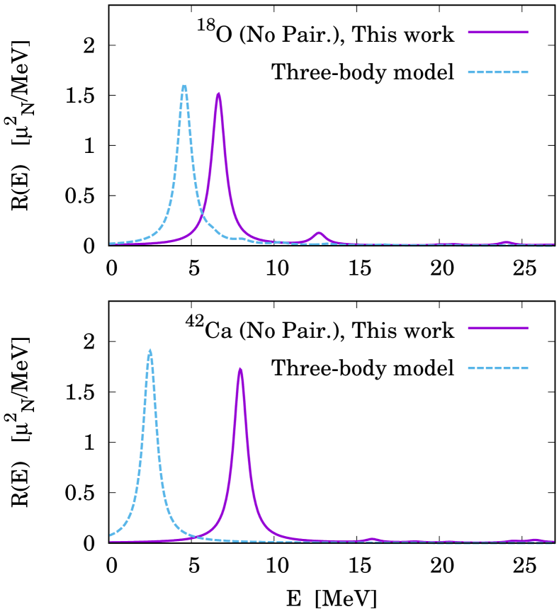
Figure 1: (Top) The M1 transition strength distributions for ¹⁸O (upper panel) and ⁴²Ca (lower panel) based on the RRPA calculations with DD-PC1 parameterization. The result from the three-body model without pairing from Ref. Oishi and Paar (2019) is shown for comparison.

Table 1: Non-energy-weighted sum ($m_{k=0}$) of the M1-response function for ¹⁸O and ⁴²Ca obtained from the RRPA calculation. The analytical SRV value from Ref. Oishi and Paar (2019) is shown for comparison. The unit is $\mu_{\rm N}^{2}$.

	$m_{0}$ (This work)	SRV Oishi and Paar (2019)
18O	$2.73$	$2.79$
42Ca	$2.91$	$2.99$

In this section, we perform the calculation of M1 SRV within the relativistic random phase approximation (RRPA), based on the formalism given in Sec. II. The DD-PC1 functional is used, supplemented with the IV-PV channel in the RRPA residual interaction, with the strength parameter $\alpha_{IV-PV}=0.53$ MeV$\cdot{\rm fm}^{3}$, as introduced in Sec. II. Note that in this sum rule test, the pairing correlations are neglected in calculations. Figure 1 displays the M1-response function $R(E)$ from Eq. (6) for ¹⁸O and ⁴²Ca, obtained with the RRPA. Our result shows the dominant single peak in each system. Table 1 shows the non-energy-weighted sum ($m_{0}$) results for M1 transitions in ¹⁸O and ⁴²Ca obtained from the RRPA. The $m_{0}$ value is calculated from Eq. (21), using the M1-strength distribution up to $50$ MeV. For comparison, the respective values introduced in Ref. Oishi and Paar (2019) are also shown as “SRV”. The RRPA accurately reproduces the SRVs for two nuclei under consideration. Namely, the relativistic framework to describe the M1 transitions appears to be valid at the level of no-pairing limit. The small deficiency of RRPA beyond the SRV value is attributable to the cutoff energy.

As shown in Fig. 1, the RRPA excitation energy of M1 mode appears rather different than in the case of three-body model from Ref. Oishi and Paar (2019). This discrepancy originates from different open-shell structures produced by the two models. For further improvement, one may adjust these models directly to the M1-reference data, which have been, however, not precisely obtained for ¹⁸O neither ⁴²Ca. Nevertheless, since the sum rule does not depend on the excitation energy, the analysis of both approaches confirms the expected M1-sum values, and thus, justifies our RRPA implementation.

III Results

In the following we present the results on M1 transitions based on the RHB+R(Q)RPA framework introduced in Sec. II. The functional DD-PC1 Nikšić et al. (2014) is systematically used in model calculations, supplemented with the pairing interaction from the phenomenological Gogny-D1S force Berger et al. (1991).

III.1 M1 transitions in ${}^{208}\rm Pb$

As the first case for detailed analysis of M1 transitions in the framework based on the RNEDF, we the consider ${}^{208}\rm Pb$ nucleus. There is experimental data on this system available Raman et al. (1977); Laszewski et al. (1977); Chrien and Kane (1979); Laszewski et al. (1985, 1988); Birkhan et al. (2016), and thus, it is suitable to the first application. Figure 2 shows the M1-response function $R_{M1}(E)$ for ${}^{208}\rm Pb$, obtained using Eq.(6). Since it is magic nucleus, pairing correlations do not contribute to the nuclear ground state energy, and the RHB + RQRPA reduces to the relativistic Hartree + RRPA model. In addition to the full response $R_{M1}(E)$, the responses to the isoscalar and isovector operators, $R_{M1}^{IS}(E)$ and $R_{M1}^{IV}(E)$, are shown separately. For comparison, the so-called “unperturbed” response at the Hartree level is also shown, corresponding to the limit when the residual RRPA interaction is set to zero.

As shown in Fig. 2, the full M1 response is dominated by the two peaks at $6.11$ MeV and $7.51$ MeV. These two peaks exhaust most of the total M1 strength up to $50$ MeV energy. In some experimental studies Laszewski et al. (1988); Birkhan et al. (2016), there has been measured a dominant peak of the M1-strength distribution around $7.0$-$7.5$ MeV, whereas the other bump could be found at $\cong 6.2$ MeV Laszewski et al. (1988). However, the experimental data also show a more fine fragmentation of the M1 strength in ²⁰⁸Pb Laszewski et al. (1988); Birkhan et al. (2016). To reproduce this fragmentation, the present RRPA may need to be improved with, e.g. the two-particle-two-hole effect Dehesa et al. (1977), which is beyond the present scope. Even with a lack of details, our RRPA scheme reproduces the rough structure of the M1-distribution of ²⁰⁸Pb, especially its dominant two-peak structure. By comparing the full-M1 response with the unperturbed response at the Hartree level (Fig. 2), one can observe that the full response is shifted to higher energies, demonstrating the effect of the IV-PV residual interaction to establish M1 transitions as genuine nuclear mode of excitation. This shift is consistent to the selection rule of M1, since the IV-PV interaction affects the $J^{\pi}=1^{+}$ excited states.

In Fig. 2, one can observe that the isovector M1 response is significantly larger than the isoscalar one, and both components interfere. The dominance of isovector mode is visible also from the M1 strength integrated up to 50 MeV: the full strength amounts $\sum B(M1)=41.99\ \mu^{2}_{N}$, whereas the isoscalar strength is $\sum B^{(IS)}(M1)=0.43\ \mu^{2}_{N}$ and the isovector strength is $\sum B^{(IV)}(M1)=42.33\ \mu^{2}_{N}$. The main reason of the isovector-M1 dominance is a large difference in the respective gyromagnetic ratios, $g_{s}^{IS}$ and $g_{s}^{IV}$ given in Eqs. (11) and (12). For more details, see Appendix A.

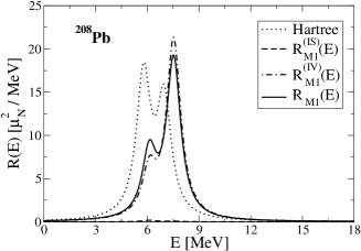
Figure 2: The M1 transition strength distribution for ²⁰⁸Pb. The results are obtained with the RRPA using the DD-PC1 functional: $R_{M1}(E)$ for full, $R^{(IS)}_{M1}(E)$ for isoscalar, and $R^{(IV)}_{M1}(E)$ for isovector response functions. Unperturbed response at the Hartree level is also shown.

Table 2: Partial neutron and proton contributions $(b_{ph}^{\nu,\pi})$ to the M1 transition strength for the two main peaks $(E_{peak})$, and respective overall transition strengths B(M1) for ²⁰⁸Pb. Details about configurations are given in the text.

$E^{th.}_{peak}[\rm MeV]$	$b_{ph}^{\nu}~{}[\mu_{N}]$	$b_{ph}^{\pi}~{}[\mu_{N}]$	$B(M1)~{}[\mu^{2}_{N}]$
6.11	$-$1.33	4.74	11.6
7.51	4.22	1.15	28.96

The structure of the two pronounced M1 peaks is analyzed in more details. Table 2 shows the respective partial contributions $b_{ph}$ to the $B({\rm M1})$ strength from the major proton and neutron particle-hole $(ph)$ configurations (see Eq. (7)). That is, if a single proton $(p_{1}h_{1})$ and neutron $(p_{2}h_{2})$ configurations contribute to the M1 transition at excitation energy $E$,

$$B({\rm M1},~{}E)=\left|b^{\nu}_{p_{1}h_{1}}(E)+b^{\pi}_{p_{2}h_{2}}(E)\right|^{2}.$$ (22)

For the state at $6.11$ MeV, the major contribution comes from the transitions between spin-orbit partner states for neutrons, $(\nu 1i^{-1}_{13/2}\rightarrow\nu 1i_{11/2})$ and protons, $(\pi 1h^{-1}_{11/2}\rightarrow\pi 1h_{9/2})$. As shown in Table 2, partial proton and partial neutron spin-flip transitions interfere destructively. In the case of the state at $7.51$ MeV, the main transitions are $(\nu 1i^{-1}_{13/2}\rightarrow\nu 1i_{11/2})$ and $(\pi 1h^{-1}_{11/2}\rightarrow\pi 1h_{9/2})$, with coherent contributions to the total B(M1) strength, as shown in Table 2.

Figure 3 shows the separation of the full M1 response in ²⁰⁸Pb to the spin and orbital response functions, $R^{\sigma}_{M1}(E)$ and $R^{\ell}_{M1}(E)$, evaluated by Eqs. (19) and (20), respectively. One can observe considerably larger spin response in comparison to the orbital one, i.e. most of the overall $B(M1)$ strength is exhausted by the spin M1 response. The orbital-M1 strength is mainly related to deformation and almost disappears in the closed-shell nuclei Heyde et al. (2010). The spin and orbital responses interfere destructively, i.e. the full response function is smaller than the spin response. The corresponding sum of the strengths amount $53.14~{}\mu^{2}_{N}$ for the spin, $1.19~{}\mu^{2}_{N}$ for the orbital, and $41.99~{}\mu^{2}_{N}$ for the full M1 transition. In the present study of ²⁰⁸Pb, the overall M1-excitation strength is almost fully exhausted by the two peaks, i.e., $B(M1,E=6.11\>{\rm MeV})=11.6\ \mu^{2}_{N}$ and $B(M1,E=7.51\>{\rm MeV})=28.96\ \mu^{2}_{N}$.

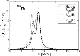
Figure 3: The same as Fig. 2, but with R(M1) - full, $R_{M1}^{\sigma}(E)$ - spin and $R^{\ell}_{M1}(E)$ - orbital response functions. Unperturbed response at the Hartree level is also shown.

Over the past years, there have been several experimental studies of M1 transitions in ²⁰⁸Pb. Several experimental results are summarized in a chronological order in Table 3. It turns out that the total measured strength lies between $\sum B(M1)\cong(35.0-47.5)\ \mu^{2}_{N}$ and it is in agreement with our result. However, from recent experiments Laszewski et al. (1985, 1988); Birkhan et al. (2016), it has also been pointed out that the actual M1 sum could need to be reduced, mainly due to the confusion with the electric-dipole components in the old experiments. A recent theoretical investigation based on the Skyrme functional Tselyaev et al. (2019) results even in lower $B(M1)$ strength in comparison to the modern experiments. Therefore, quantitative description of the transition strengths for M1 modes remains an open question. In comparison to Bohr and Mottelson’s independent particle model (IPM), which estimates $B(M1)=36\ \mu^{2}_{N}$ in Ref. Laszewski and Axel (1979), the RRPA result is comparable, but somewhat higher. In Refs. Vesely et al. (2009); Nesterenko et al. (2010); Tselyaev et al. (2019), the similar calculation based on the Skyrme functionals have been used, with the quenching factors in $g$ coefficients, $\simeq$ 0.65, in order to reduce the transition strength. When using the quenching, the total B(M1) strength for ²⁰⁸Pb obtained for a set of Skyrme parameterizations amounts 14.8-17.3 $\mu^{2}_{N}$ Vesely et al. (2009).

Table 3: A summary of reported experimental M1 excitation energies and transition strengths in ${}^{208}\rm Pb$. In Ref. Chrien and Kane (1979), the symbol (*) denotes experimental ambiguity due to parity assignment to the quantum mechanical state with respect to M1 transitions.

(208Pb)	$E_{x}[\rm MeV]$	$B_{M1,~{}\uparrow}[\mu^{2}_{N}]$
Ref. Raman et al. (1977) (1977)	(sum)	$35.0$
Ref. Laszewski et al. (1977) (1977)	(sum)	$46.5$
Ref. Chrien and Kane (1979) (1979)	$4.843$	$5.8^{*}$
	$7.061$	$17.7^{*}$
	$7.249$	$0.5$
	$7.37-7.82$	$7.9$
	$7.98$	$7.1^{*}$
	$8.20-9.50$	$8.5$
	$4.843-9.50$	$\sum B(M1,E)_{\uparrow}$
		$=47.5~{}(30.6^{*})$
Ref. Laszewski et al. (1985) (1985)	$5.8-7.4$	$10.7$
	$\leq 6.4$	$1.9$
	7.3	$15.6$
Ref. Laszewski et al. (1988) (1988)	$6.7-8.1$	$19.0$
Ref. Birkhan et al. (2016) (2016)	$7.0-9.0$	$20.5$

III.2 M1 transitions in ${}^{48}\rm Ca$

In the following, we extend our study to the lighter system, ${}^{48}\rm Ca$ nucleus, where several experimental data are available Birkhan et al. (2016); Yako et al. (2009); Tompkins et al. (2011). In Fig. 4, the RRPA full, isoscalar, and isovector $B(M1)$ transition-strength distributions are shown for ${}^{48}\rm Ca$. The M1 strength distribution is composed from a single dominant peak. The corresponding transition strength summed up to $50$ MeV amounts $B(M1)$ = 10.38 $\ \mu^{2}_{N}$ (total), $B^{(IS)}(M1)$ = 0.11 $\ \mu^{2}_{N}$ and $B^{(IV)}(M1)$ = 12.52 $\ \mu^{2}_{N}$. Similarly as in the case of ²⁰⁸Pb, the isovector strength is larger than the isoscalar one. The centroid and peak energies of the full response are $\bar{E}^{th.}=9.37\ \rm MeV$ and $E^{th.}_{peak}=8.48\ \rm MeV$, respectively. On the other side, in the experimental investigation of M1 spin-flip resonance from inelastic proton scattering on ${}^{48}\rm Ca$ Birkhan et al. (2016), the dominant peak locates at slightly higher energy, $E^{exp.}_{peak}=10.22\ \rm MeV$. We note that the present IV-PV interaction, which controls the M1-excited state of $1^{+}$ configuration, is described with the simple, constant coupling. By comparing the full response with the unperturbed one, the RRPA residual interaction shifts the main peak toward higher energy (Fig. 4). This is similar as shown in the ²⁰⁸Pb case, demonstrating the effect of the residual RRPA interaction.

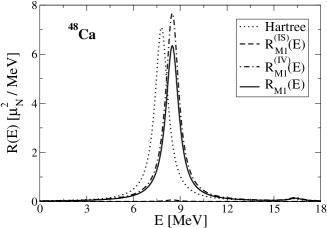
Figure 4: The same as Fig. 2, but for ${}^{48}\rm Ca$.

Figure 5 shows the full, spin and orbital-M1 transition strength distributions for ${}^{48}\rm Ca$. The corresponding $B(M1)$ values are $10.38~{}\mu^{2}_{N}$, $10.40~{}\mu^{2}_{N}$, and $5.35\times 10^{-3}~{}\mu^{2}_{N}$, respectively. Similarly as in the case of heavy system ²⁰⁸Pb, the spin transition strength dominates, i.e., it is four orders of magnitude larger than the orbital strength, $B^{\sigma}(M1)\gg B^{\ell}(M1)$.

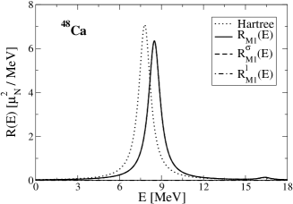
Figure 5: The same as Fig. 3 but for ${}^{48}\rm Ca$. The spin and full response functions coincide.

From the analysis of the major M1 state at $8.48$ MeV, we confirmed that it is composed mainly from the transition between the neutron spin-orbit partner states, $(\nu 1f^{-1}_{7/2}\rightarrow\nu 1f_{5/2})$. The major partial neutron and proton contributions to the B(M1) strength are presented in Table 4, showing the dominance of the neutron spin-flip transitions over the proton ones.

Table 4: Partial neutron and proton contributions $(b_{ph}^{\nu,\pi})$ to the M1 transition strength and the full transition strength $B({\rm M1})$ for the major peak at 8.48 MeV for ⁴⁸Ca.

$E^{th.}_{peak}[\rm MeV]$	$b_{ph}^{\nu}[\mu_{N}]$	$b_{ph}^{\pi}[\mu_{N}]$	$B(M1)[\mu^{2}_{N}]$
8.48	3.18	$4.04\times 10^{-4}$	9.96

In the experimental investigation of M1 spin-flip resonance from inelastic proton scattering on ${}^{48}\rm Ca$ Birkhan et al. (2016), the dominant peak at $E^{exp.}_{peak}=10.22\ \rm MeV$ is of pure neutron character, dominated by the transition $(\nu 1f^{-1}_{7/2}\rightarrow\nu 1f_{5/2})$. This character is consistent as obtained in the present study. The measured strength is obtained as $\sum B(M1)=3.85$-$4.63~{}\mu^{2}_{N}$ Birkhan et al. (2016). In Ref. Birkhan et al. (2016), the data on ${}^{48}{\rm Ca}(p,n)$ reaction Yako et al. (2009) have also been reanalyzed, resulting with $\sum B(M1)=3.45$-$4.10~{}\mu^{2}_{N}$. Comparison with the RRPA results from the present analysis, $\sum B(M1)$ = 10.38 $\mu^{2}_{N}$, indicates the enhancement of the theoretical prediction for the $B(M1)$ transition strength. We note that another experimental study, based on $(\gamma,n)$ reaction Tompkins et al. (2011), resulted in twice as large value than in $(p,p^{\prime})$ reaction Birkhan et al. (2016), $B(M1)=6.8\pm 0.5~{}\mu^{2}_{N}$. This measurement is closer, but still below the result of our present work. One possibility to remove this discrepancy is by introducing the quenching factor $\eta\simeq 0.6-0.7$ for the $g_{s,\ell}$ coefficients. In this case, our sum of the B(M1) strength changes as $\sum B(M1)\longrightarrow\eta^{2}\sum B(M1)\simeq 3.7-5.1~{}\mu^{2}_{N}$. Note that the similar quenching factors have been utilized in several theoretical calculations Vesely et al. (2009); Nesterenko et al. (2010). For example, a study based on Skyrme functionals results in B(M1) values 2.5-4.8 $\mu^{2}_{N}$ Vesely et al. (2009).

Table 5: The peak energies $E^{th.}_{peak}$ and corresponding $B(M1)$ values for ${}^{42}\rm Ca$ and ⁵⁰Ti in this work.

Nuclides	Method	$E^{th.}_{peak}[\rm MeV]$	$B(M1)[\mu^{2}_{N}]$
42Ca	RRPA	7.95	2.92
	RQRPA	11.32	2.12
50Ti	RRPA	8.82	13.86
	RQRPA	8.58	8.53
		11.57	3.88

III.3 Pairing effects on M1 transitions

In this section we apply the complete RHB + RQRPA framework adopted for the description of M1 transitions in open-shell nuclei, by consistent implementation of the pairing correlations in the nuclear ground state and in the RQRPA residual interaction. The main purpose here is to explore the role of the pairing correlations on the properties of the M1 response. The sensitivity of the M1 transitions on pairing correlations has previously been addressed in the study based on the three-body model Oishi and Paar (2019). In the present study, we discuss the same aspect, but utilizing a microscopic RNEDF approach.

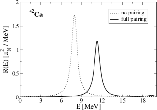
Figure 6: The RHB + RQRPA response for M1 transitions in ${}^{42}\rm Ca$ using the DD-PC1 parameterization and Gogny pairing correlations. The response functions without pairing correlations (RRPA) and with full pairing (RQRPA) are shown separately.

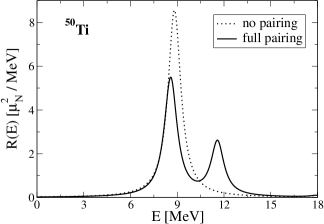
Figure 7: The same as Fig. 6 but for ${}^{50}\rm Ti$.

As the first open-shell system we study ${}^{42}\rm Ca$, which is already considered in its no-pairing limit in Sec. II.3 in order to verify the M1 sum rule in the core-plus-two-nucleon system Oishi and Paar (2019). In Fig. 6, the results of the full RHB + RQRPA calculation are shown, in comparison to the limit without pairing correlations both in the ground state (GS) and in the residual interaction. The full-RQRPA M1 response shows one major peak at $11.32$ MeV, that is composed mainly by a single-neutron $2qp$ transition, $(\nu 1f^{-1}_{7/2}\rightarrow\nu 1f_{5/2})$. In comparison to the peak obtained in RRPA calculation without pairing correlations, the pairing interaction shifts the resonant peak by several MeV to higher energies and reduces its strength. This shift by the pairing correlations at the quantitative level can also be seen in Table 5. The present result is consistent to that in Ref. Oishi and Paar (2019): the pairing interaction, which promotes the spin-singlet pairing between the valence nucleons, shifts the M1-excitation energy toward higher region, with a reduction of the strength, $B(M1)$. We note that the pairing effect in the particle-particle channel of the residual RQRPA interaction is finite but very small for the M1 transition from the $0^{+}$ GS to $1^{+}$ excited states. The major pairing effects originate from the properties of the GS. The same effect has been theoretically observed for the surface delta interaction applied on the M1 excitations in the particle-particle channel Tanimura et al. (2012).

Next we move to the ⁵⁰Ti nucleus, where the M1-excitations from its GS have been measured Sober et al. (1985). These data can be utilized as reference to infer the present accuracy and drawback of the RQRPA calculations. In Fig. 7, our result is presented in the case of calculations with and without pairing correlations. The respective properties of M1 transitions are tabulated in Table 5. In the ⁵⁰Ti case, the pairing interaction causes the main peak to split into two: $E^{th.}_{peak}=8.58$ and $11.57$ MeV. This two-peak structure has been confirmed in the experiments at $E^{exp.}_{peak}\cong 8.7$ and $10.2$ MeV Sober et al. (1985). Thus, the RQRPA reasonably reproduces the general structure of M1 excitation spectrum. Considering the deviation of calculated energies from the empirical values, further development and/or optimization of the RNEDF is required. Note also that, as we already discussed in the previous sections, the actual data from experiments suggests a more fine fragmentation, for which complicated additional effects may need to be considered, e.g., the meson-exchange current effect Heyde et al. (2010); Richter (1990); Richter et al. (1990); Moraghe et al. (1994); Marcucci et al. (2008); Schwengner et al. (2017) and/or the second-order (Q)RPA Dehesa et al. (1977); Bertsch and Hamamoto (1982); Ichimura et al. (2006).

The RQRPA calculations show that the two main M1 peaks in ⁵⁰Ti mainly originate from the proton transition of $(\pi 1f^{-1}_{7/2}\rightarrow\pi 1f_{5/2})$ and neutron transition of $(\nu 1f^{-1}_{7/2}\rightarrow\nu 1f_{5/2})$. This is because of the shell closure at $Z=N=20$, thus the main M1-excitation components are attributed to the valence, two protons and eight neutrons in the $1f_{7/2}$ orbit.

IV Summary

In this work we have introduced a novel approach to describe M1 transitions in nuclei, based on the RHB + RQRPA framework with the relativistic point-coupling interaction, supplemented with the pairing correlations described by the pairing part of the Gogny force. In addition to the standard terms of the point coupling model with the DD-PC1 parameterization, the residual R(Q)RPA interaction has been extended by the isovector-pseudovector contact type of interaction that contributes to unnatural parity transitions. A recently developed non-pairing M1 sum rule in core-plus-two-nucleon systems Oishi and Paar (2019) has been used as a consistency check of the present theory framework. The sum of the M1-transition strength for ${}^{42}\rm Ca$ accurately reproduced the sum rule value (SRV), thus validating the introduced formalism and its numerical implementation for further exploration of M1 transitions.

The present framework is first benchmarked on M1 transitions for two magic nuclei, ⁴⁸Ca and ²⁰⁸Pb. The response functions $B(M1,E)$ have been explored in details, including their isoscalar and isovector components, that relate to the electromagnetic probe, as well as contributions of the spin and orbital components of the M1 transition operator. It is confirmed that, in nuclei without deformation, the spin component of the M1 transition strength dominates over the orbital one. Due to the differences in the gyromagnetic ratios, the isovector M1 transition strength is significantly larger than the isoscalar one, and they interfere destructively. It is shown that the major peaks of isovector spin-M1 transitions are dominated mainly by a single $ph$ configuration composed of spin-orbit partner states.

One of our interests was to investigate the role of the pairing correlations on the properties of M1 response functions in open shell nuclei, that has been addressed in the study of ⁴²Ca and ⁵⁰Ti. The RQRPA calculations show a significant impact of pairing correlations on the major peak by shifting it to the higher energies, and at the same time, by reducing the transition strength. In the ⁵⁰Ti case, this effect is essential to reproduce the two-peak structure measured in the experiment Sober et al. (1985). The main effect of the pairing correlations is observed at the level of the ground state calculation, while it is rather small in the particle-particle channel of the residual RQRPA interaction.

The M1 transition strengths from the present study appear larger than the values obtained from the experimental data. Therefore, it remains open question whether some additional effects should be included at the theory side, or some strength may be missing in the experimental data. In addition, the M1-excitation energies of light systems, e.g. ⁴⁸Ca still have some deviation from the reference data. In order to resolve these open questions, further developments are needed, e.g., resolving the quenching effects in $g$ factors, meson exchange effects, couplings with complex configurations, etc. Due to its relation to the spin-orbit interaction, M1 excitations could also provide a guidance toward more advanced RNEDFs. Recently, a new relativistic energy density functional has been constrained not only by the ground state properties of nuclei, but also by using the E1 excitation properties (i.e. dipole polarizability) and giant monopole resonance energy in ²⁰⁸Pb Yüksel et al. (2019). Similarly, M1 excitation properties in selected nuclei could also be exploited in the future studies to improve the RNEDFs.

Appendix A Isoscalar-isovector (IS-IV) decomposition

In this appendix we give some details on the IS-IV decomposition of the transition operator in a general consideration that applies both to electric and magnetic transitions. Namely, we consider the $X\lambda\mu$ transition, where $X$ denotes $E$ or $M$ for electric and magnetic transitions, respectively, and $(\lambda,~{}-\lambda<\mu<\lambda)$ denote the multipole quantum numbers. The $A$-body operator of the $X\lambda\mu$ transition is given as

$$\hat{\mathcal{P}}(X\lambda\mu)=\sum_{i=1}^{A}\hat{\mathcal{Q}}(X\lambda\mu;i),$$ (23)

where $\hat{\mathcal{Q}}$ is the general single-particle operator. Then, by using the isospin $\tau_{3}=+1~{}(-1)$ for protons (neutrons), it is expressed as

$$\hat{\mathcal{P}}(X\lambda\mu) = \sum_{k\in Z}f^{\pi}_{X\lambda}\hat{\mathcal{S}}(X\lambda\mu;\bm{r}_{k})+\sum_{l\in N}f^{\nu}_{X\lambda}\hat{\mathcal{S}}(X\lambda\mu;\bm{r}_{l}),$$ (24)

$$= \sum_{i=1}^{A}\left[f^{\pi}_{X\lambda}\frac{1+\hat{\tau_{3}}(i)}{2}+f^{\nu}_{X\lambda}\frac{1-\hat{\tau_{3}}(i)}{2}\right]$$

$$~{}~{}~{}~{}\cdot\hat{\mathcal{S}}(X\lambda\mu;\bm{r}_{i}),$$

where $f^{\pi~{}(\nu)}_{X\lambda}$ indicates the charge (for $E\lambda$) or gyromagnetic factor (for $M\lambda$) of the $X\lambda$ mode for protons (neutrons), and $\hat{\mathcal{S}}(X\lambda\mu;\bm{r}_{i})$ is the transition operator. See Table 6 for some examples for E2 and M1 transitions Ring and Schuck (1980).

Table 6: The transition operators and respective proportionality factors for E2 and M1 (orbital and spin part) modes Ring and Schuck (1980). See text for details.

$X\lambda$	$(f^{\pi},~{}f^{\nu})$	$(f^{IS},~{}f^{IV})$	$\hat{\mathcal{S}}(\bm{r})$
$E2$	$(e,~{}0)$	$(e/2,~{}e/2)$	$r^{2}Y_{2\mu}(\bar{\bm{r}})$
$M1,~{}l$	$(g^{\pi}_{l},~{}g^{\nu}_{l})$	$(g^{IS}_{l},~{}g^{IV}_{l})$	$\mu_{\rm N}(\bm{\hat{l}}\cdot\bm{r}/r)_{\mu}$
	$=(1,~{}0)$	$=(1/2,~{}1/2)$	$\times\sqrt{3/4\pi}$
$M1,~{}s$	$(g^{\pi}_{s},~{}g^{\nu}_{s})$	$(g^{IS}_{s},~{}g^{IV}_{s})$	$\mu_{\rm N}(\bm{\hat{s}}\cdot\bm{r}/r)_{\mu}$
	$=(5.586,-3.826)$	$=(0.880,~{}4.706)$	$\times\sqrt{3/4\pi}$

From Eq. (24), the IS-IV decomposition is derived:

$$\hat{\mathcal{P}}(X\lambda\mu)=\hat{\mathcal{P}}^{IS}(X\lambda\mu)+\hat{\mathcal{P}}^{IV}(X\lambda\mu)$$

$$=f^{IS}_{X\lambda}\sum_{i=1}^{A}\hat{\mathcal{S}}(X\lambda\mu;\bm{r}_{i})+f^{IV}_{X\lambda}\sum_{i=1}^{A}\hat{\mathcal{S}}(X\lambda\mu;\bm{r}_{i})\hat{\tau_{3}}(i).$$ (25)

Omitting the subscript $X\lambda$ for simplicity, the $f^{IS}$ and $f^{IV}$ factors are determined as

$$f^{IS}=\frac{f^{\pi}+f^{\nu}}{2},~{}~{}f^{IV}=\frac{f^{\pi}-f^{\nu}}{2},$$ (26)

and equivalently, $f^{\pi}=f^{IS}+f^{IV}$, and $f^{\nu}=f^{IS}-f^{IV}$. It is useful to check the relation between the proton-neutron and IS-IV decompositions. That is, by using $\hat{\mathcal{X}}^{\pi}=\sum\limits_{k\in Z}\hat{\mathcal{S}}(X\lambda\mu;k)$ and $\hat{\mathcal{X}}^{\nu}=\sum\limits_{l\in N}\hat{\mathcal{S}}(X\lambda\mu;l)$,

$$\hat{\mathcal{P}}^{IS}(X\lambda\mu) = f^{IS}\left[\hat{\mathcal{X}}^{\pi}+\hat{\mathcal{X}}^{\nu}\right],$$

$$\hat{\mathcal{P}}^{IV}(X\lambda\mu) = f^{IV}\left[\hat{\mathcal{X}}^{\pi}-\hat{\mathcal{X}}^{\nu}\right],$$ (27)

where we have implemented $\tau_{3}=-1$ for neutrons in the last term. Then, it is worthwhile to consider some special cases as follows.

First we assume that only the neutron component is active for the transition, namely, $\Braket{f}{\hat{\mathcal{X}}^{\pi}}{i}\cong 0$ and $\Braket{f}{\hat{\mathcal{X}}^{\nu}}{i}\neq 0$, like as the ⁴⁸Ca result in the main text. In this case, if $f^{IS}\ll f^{IV}$ likely as spin-M1, the corresponding IV mode becomes dominant. That is,

$$\left|\Braket{f}{\hat{\mathcal{P}}^{IS}}{i}\right|^{2} \ll \left|\Braket{f}{\hat{\mathcal{P}}^{IV}}{i}\right|^{2}$$ (28)

$$\cong\left|f^{IV}\right|^{2}\left|\Braket{f}{\hat{\mathcal{X}}^{\nu}}{i}\right|^{2}.$$

Otherwise, if $f^{IS}\cong f^{IV}$ likely as E2 and orbit-M1,

$$\left|\Braket{f}{\hat{\mathcal{P}}^{IS}}{i}\right|^{2}\cong\left|\Braket{f}{\hat{\mathcal{P}}^{IV}}{i}\right|^{2}.$$ (29)

Note also that, by considering the IS+IV response,

$$\Braket{f}{\hat{\mathcal{P}}^{IS}+\hat{\mathcal{P}}^{IV}}{i} = f^{\pi}\Braket{f}{\hat{\mathcal{X}}^{\pi}}{i}+f^{\nu}\Braket{f}{\hat{\mathcal{X}}^{\nu}}{i}$$ (30)

$$\cong 0+f^{\nu}\Braket{f}{\hat{\mathcal{X}}^{\nu}}{i},$$

then, this response vanishes when $f^{\nu}=0$, as in the E2 and orbit-M1 cases. In Fig. 5 for ⁴⁸Ca, indeed the orbit-M1 response is zero, and the total and spin-M1 results coincide.

Next, when the proton and neutron excitations occur in the same phase, it means

$$\Braket{f}{\hat{\mathcal{X}}^{\nu}}{i}\propto(+)\Braket{f}{\hat{\mathcal{X}}^{\pi}}{i},$$ (31)

and thus,

$$\left|\Braket{f}{\hat{\mathcal{X}}^{\pi}-\hat{\mathcal{X}}^{\nu}}{i}\right|^{2}\ll\left|\Braket{f}{\hat{\mathcal{X}}^{\pi}+\hat{\mathcal{X}}^{\nu}}{i}\right|^{2}.$$ (32)

In this case, as long as $f^{IS}\cong f^{IV}$, the IS mode is obviously dominant. Otherwise, the result can depend on the competition of the $f^{IS}/f^{IV}$ ratio against the weightless amplitudes in Eq. (32). Note also that, for this problem, the quantities $\Braket{f}{\hat{\mathcal{X}}^{\pi}}{i}$ and $\Braket{f}{\hat{\mathcal{X}}^{\nu}}{i}$ noticeably depend on the number of protons and neutrons, as well as the specific form of the transition operator. In our results in the main text, for the spin-M1 mode, the IV component is concluded as dominant commonly for the nuclides discussed. This result is mainly attributed to that the factor $f^{IV}=g^{IV}_{s}$ is sufficiently larger than $f^{IS}=g^{IS}_{s}$.

Finally, when the proton and neutron excitations occur in the opposite phase, $\Braket{f}{\hat{\mathcal{X}}^{\nu}}{i}\propto(-)\Braket{f}{\hat{\mathcal{X}}^{\pi}}{i}$, and thus,

$$\left|\Braket{f}{\hat{\mathcal{X}}^{\pi}-\hat{\mathcal{X}}^{\nu}}{i}\right|^{2}\gg\left|\Braket{f}{\hat{\mathcal{X}}^{\pi}+\hat{\mathcal{X}}^{\nu}}{i}\right|^{2}.$$ (33)

In this case, the IV transition becomes dominant in the E2, orbit-M1, and spin-M1 cases, anyway.

References

- Richter (1985) A. Richter, Progress in Particle and Nuclear Physics 13, 1 (1985).
- Richter (1995) A. Richter, Progress in Particle and Nuclear Physics 34, 261 (1995).
- Heyde et al. (2010) K. Heyde, P. von Neumann-Cosel, and A. Richter, Rev. Mod. Phys. 82, 2365 (2010).
- Kneissl et al. (1996) U. Kneissl, H. Pitz, and A. Zilges, Progress in Particle and Nuclear Physics 37, 349 (1996).
- Pietralla et al. (2008) N. Pietralla, P. von Brentano, and A. Lisetskiy, Progress in Particle and Nuclear Physics 60, 225 (2008).
- Shizuma et al. (2008) T. Shizuma, T. Hayakawa, H. Ohgaki, H. Toyokawa, T. Komatsubara, N. Kikuzawa, A. Tamii, and H. Nakada, Phys. Rev. C 78, 061303 (2008).
- Goriely (2015) S. Goriely, Nuclear Physics A 933, 68 (2015).
- Goriely et al. (2016) S. Goriely, S. Hilaire, S. Péru, M. Martini, I. Deloncle, and F. Lechaftois, Phys. Rev. C 94, 044306 (2016).
- Langanke et al. (2004) K. Langanke, G. Martínez-Pinedo, P. von Neumann-Cosel, and A. Richter, Phys. Rev. Lett. 93, 202501 (2004), and references therein.
- Langanke and Martínez-Pinedo (2003) K. Langanke and G. Martínez-Pinedo, Rev. Mod. Phys. 75, 819 (2003).
- Langanke et al. (2008) K. Langanke, G. Martínez-Pinedo, B. Müller, H.-T. Janka, A. Marek, W. R. Hix, A. Juodagalvis, and J. M. Sampaio, Phys. Rev. Lett. 100, 011101 (2008).
- Loens et al. (2012) H. P. Loens, K. Langanke, G. Martinez-Pinedo, and K. Sieja, The European Physical Journal A 48, 34 (2012).
- Chadwick and et. al. (2011) M. B. Chadwick and et. al., Nuclear Data Sheets 112, 2887 (2011).
- Otsuka et al. (2005) T. Otsuka, T. Suzuki, R. Fujimoto, H. Grawe, and Y. Akaishi, Phys. Rev. Lett. 95, 232502 (2005).
- Otsuka et al. (2010) T. Otsuka, T. Suzuki, M. Honma, Y. Utsuno, N. Tsunoda, K. Tsukiyama, and M. Hjorth-Jensen, Phys. Rev. Lett. 104, 012501 (2010).
- Vesely et al. (2009) P. Vesely, J. Kvasil, V. O. Nesterenko, W. Kleinig, P. G. Reinhard, and V. Y. Ponomarev, Phys. Rev. C 80, 031302 (2009).
- Nesterenko et al. (2010) V. O. Nesterenko, J. Kvasil, P. Vesely, W. Kleinig, P.-G. Reinhard, and V. Y. Ponomarev, Journal of Physics G: Nuclear and Particle Physics 37, 064034 (2010).
- Tselyaev et al. (2019) V. Tselyaev, N. Lyutorovich, J. Speth, P.-G. Reinhard, and D. Smirnov, Phys. Rev. C 99, 064329 (2019).
- Vergados et al. (2012) J. D. Vergados, H. Ejiri, and F. Šimkovic, Reports on Progress in Physics 75, 106301 (2012).
- Arteaga and Ring (2008) D. P. Arteaga and P. Ring, Phys. Rev. C 77, 034317 (2008).
- Ebran et al. (2011) J.-P. Ebran, E. Khan, D. Peña Arteaga, and D. Vretenar, Phys. Rev. C 83, 064323 (2011).
- Richter (1990) A. Richter, Nuclear Physics A 507, 99 (1990).
- Otsuka (1990) T. Otsuka, Nuclear Physics A 507, 129 (1990).
- Bohle et al. (1984a) D. Bohle, A. Richter, W. Steffen, A. Dieperink, N. L. Iudice, F. Palumbo, and O. Scholten, Physics Letters B 137, 27 (1984a).
- Bohle et al. (1984b) D. Bohle, G. Küchler, A. Richter, and W. Steffen, Physics Letters B 148, 260 (1984b).
- Schwengner et al. (2017) R. Schwengner, S. Frauendorf, and B. A. Brown, Phys. Rev. Lett. 118, 092502 (2017).
- Balbutsev et al. (2018) E. B. Balbutsev, I. V. Molodtsova, and P. Schuck, Phys. Rev. C 97, 044316 (2018).
- Repko et al. (2019) A. Repko, J. Kvasil, and V. O. Nesterenko, Phys. Rev. C 99, 044307 (2019).
- Oishi and Paar (2019) T. Oishi and N. Paar, Phys. Rev. C 100, 024308 (2019).
- Dang and Hung (2013) N. D. Dang and N. Q. Hung, J. Phys. G: Nucl. Part. Phys. 40, 105103 (2013).
- Yoshida (2009) K. Yoshida, Phys. Rev. C 80, 044324 (2009).
- Terasaki and Engel (2011) J. Terasaki and J. Engel, Phys. Rev. C 84, 014332 (2011).
- Ebata et al. (2014) S. Ebata, T. Nakatsukasa, and T. Inakura, Phys. Rev. C 90, 024303 (2014).
- Stetcu et al. (2011) I. Stetcu, A. Bulgac, P. Magierski, and K. J. Roche, Phys. Rev. C 84, 051309 (2011).
- Tamii et al. (2007) A. Tamii et al., Nucl. Phys. A 788, 53 (2007).
- Fujita et al. (2011a) Y. Fujita, B. Rubio, and W. Gelletly, Prog. Part. Nucl. Phys. 66, 549 (2011a).
- Birkhan et al. (2016) J. Birkhan, H. Matsubara, P. von Neumann-Cosel, N. Pietralla, V. Y. Ponomarev, A. Richter, A. Tamii, and J. Wambach, Phys. Rev. C 93, 041302 (2016).
- Laszewski et al. (1988) R. M. Laszewski, R. Alarcon, D. S. Dale, and S. D. Hoblit, Phys. Rev. Lett. 61, 1710 (1988).
- Laszewski et al. (1985) R. M. Laszewski, P. Rullhusen, S. D. Hoblit, and S. F. LeBrun, Phys. Rev. Lett. 54, 530 (1985).
- Laszewski and Axel (1979) R. M. Laszewski and P. Axel, Phys. Rev. C 19, 342 (1979).
- Laszewski et al. (1977) R. M. Laszewski, R. J. Holt, and H. E. Jackson, Phys. Rev. Lett. 38, 813 (1977).
- Chrien and Kane (1979) R. E. Chrien and W. R. Kane, Neutron Capture Gamma-Ray Spectroscopy (Springer-Verlag US, 1979).
- Raman et al. (1977) S. Raman, M. Mizumoto, and R. L. Macklin, Phys. Rev. Lett. 39, 598 (1977).
- Sieja (2018) K. Sieja, Phys. Rev. C 98, 064312 (2018).
- Maripuu (1969) S. Maripuu, Nuclear Physics A 123, 357 (1969).
- Kurath (1963) D. Kurath, Phys. Rev. 130, 1525 (1963).
- Migli et al. (1991) E. Migli, S. Drozdz, J. Speth, and J. Wambach, Z. Phys. A 340, 111 (1991).
- Kamerdzhiev et al. (1993) S. Kamerdzhiev, J. Speth, G. Tertychny, and J. Wambach, Zeitschrift für Physik A 346, 253 (1993).
- Moraghe et al. (1994) S. Moraghe, J. Amaro, C. García-Recio, and A. Lallena, Nuclear Physics A 576, 553 (1994).
- Marcucci et al. (2008) L. E. Marcucci, M. Pervin, S. C. Pieper, R. Schiavilla, and R. B. Wiringa, Phys. Rev. C 78, 065501 (2008).
- Cao et al. (2009) L.-G. Cao, G. Colò, H. Sagawa, P. F. Bortignon, and L. Sciacchitano, Phys. Rev. C 80, 064304 (2009).
- Speth et al. (2020) J. Speth, P.-G. Reinhard, V. Tselyaev, and N. Lyutorovich, arXiv (2020).
- Vretenar et al. (2005) D. Vretenar, A. V. Afanasjev, G. A. Lalazissis, and P. Ring, Phys. Rep. 409, 101 (2005).
- Nikšić et al. (2005) T. Nikšić, T. Marketin, D. Vretenar, N. Paar, and P. Ring, Phys. Rev. C 71, 014308 (2005).
- Paar et al. (2007) N. Paar, D. Vretenar, E. Khan, and G. Colò, Reports on Progress in Physics 70, 691 (2007).
- Paar et al. (2008) N. Paar, D. Vretenar, T. Marketin, and P. Ring, Phys. Rev. C 77, 024608 (2008).
- Niu et al. (2009) Y. Niu, N. Paar, D. Vretenar, and J. Meng, Physics Letters B 681, 315 (2009).
- Khan et al. (2011) E. Khan, N. Paar, and D. Vretenar, Phys. Rev. C 84, 051301 (2011).
- Paar et al. (2014) N. Paar, C. C. Moustakidis, T. Marketin, D. Vretenar, and G. A. Lalazissis, Phys. Rev. C 90, 011304 (2014).
- Roca-Maza et al. (2015) X. Roca-Maza, N. Paar, and G. Colò, Journal of Physics G: Nuclear and Particle Physics 42, 034033 (2015).
- Nikšić et al. (2015) T. Nikšić, N. Paar, P.-G. Reinhard, and D. Vretenar, Journal of Physics G: Nuclear and Particle Physics 42, 034008 (2015).
- Paar et al. (2015) N. Paar, T. Marketin, D. Vale, and D. Vretenar, Int. J. Mod. Phys. E 24, 1541004 (2015).
- Vale et al. (2016) D. Vale, T. Rauscher, and N. Paar, J. Cosm. Astr. Phys. 2, 007 (2016).
- Roca-Maza and Paar (2018) X. Roca-Maza and N. Paar, Progress in Particle and Nuclear Physics 101, 96 (2018).
- Nikšić et al. (2014) T. Nikšić, N. Paar, D. Vretenar, and P. Ring, Computer Physics Communications 185, 1808 (2014).
- Yüksel et al. (2019) E. Yüksel, T. Marketin, and N. Paar, Phys. Rev. C 99, 034318 (2019).
- Pai et al. (2016) H. Pai, T. Beck, J. Beller, R. Beyer, M. Bhike, V. Derya, U. Gayer, J. Isaak, Krishichayan, J. Kvasil, B. Löher, V. O. Nesterenko, N. Pietralla, G. Martínez-Pinedo, L. Mertes, V. Y. Ponomarev, P.-G. Reinhard, A. Repko, P. C. Ries, C. Romig, D. Savran, R. Schwengner, W. Tornow, V. Werner, J. Wilhelmy, A. Zilges, and M. Zweidinger, Phys. Rev. C 93, 014318 (2016).
- Nikšić et al. (2008) T. Nikšić, D. Vretenar, and P. Ring, Phys. Rev. C 78, 034318 (2008).
- Berger et al. (1991) J. F. Berger, M. Girod, and D. Gogny, Computer Physics Communications 63, 365 (1991).
- Paar et al. (2003) N. Paar, P. Ring, T. Nikšić, and D. Vretenar, Phys. Rev. C 67, 034312 (2003).
- Nikšić et al. (2002) T. Nikšić, D. Vretenar, and P. Ring, Phys. Rev. C 66, 064302 (2002).
- Lipparini et al. (1976) E. Lipparini, S. Stringari, M. Traini, and R. Leonardi, Il Nuovo Cimento A (1965-1970) 31, 207 (1976).
- Fujita et al. (2011b) Y. Fujita, B. Rubio, and W. Gelletly, Progress in Particle and Nuclear Physics 66, 549 (2011b).
- Sagawa et al. (2019) H. Sagawa, G. Colò, X. Roca-Maza, and Y. Niu, The European Physical Journal A 55, 227 (2019).
- Love and Franey (1983) W. G. Love and M. A. Franey, Phys. Rev. C 27, 438 (1983).
- Dehesa et al. (1977) J. S. Dehesa, J. Speth, and A. Faessler, Phys. Rev. Lett. 38, 208 (1977).
- Speth and van der Woude (1981) J. Speth and A. van der Woude, Reports on Progress in Physics 44, 719 (1981).
- Suzuki (1984) T. Suzuki, J. Phys. Colloques 45, 251 (1984).
- Liu et al. (1991) K.-F. Liu, H.-D. Luo, Z. Ma, M. Feng, and Q.-B. Shen, Nuclear Physics A 534, 48 (1991).
- Osterfeld (1992) F. Osterfeld, Rev. Mod. Phys. 64, 491 (1992).
- Weisskopf (1951) V. F. Weisskopf, Phys. Rev. 83, 1073 (1951).
- Ring and Schuck (1980) P. Ring and P. Schuck, The Nuclear Many-Body Problems (Springer-Verlag, Berlin and Heidelberg, Germany, 1980).
- Yako et al. (2009) K. Yako, M. Sasano, K. Miki, H. Sakai, M. Dozono, D. Frekers, M. B. Greenfield, K. Hatanaka, E. Ihara, M. Kato, T. Kawabata, H. Kuboki, Y. Maeda, H. Matsubara, K. Muto, S. Noji, H. Okamura, T. H. Okabe, S. Sakaguchi, Y. Sakemi, Y. Sasamoto, K. Sekiguchi, Y. Shimizu, K. Suda, Y. Tameshige, A. Tamii, T. Uesaka, T. Wakasa, and H. Zheng, Phys. Rev. Lett. 103, 012503 (2009).
- Tompkins et al. (2011) J. R. Tompkins, C. W. Arnold, H. J. Karwowski, G. C. Rich, L. G. Sobotka, and C. R. Howell, Phys. Rev. C 84, 044331 (2011).
- Tanimura et al. (2012) Y. Tanimura, K. Hagino, and H. Sagawa, Phys. Rev. C 86, 044331 (2012).
- Sober et al. (1985) D. I. Sober, B. C. Metsch, W. Knüpfer, G. Eulenberg, G. Küchler, A. Richter, E. Spamer, and W. Steffen, Phys. Rev. C 31, 2054 (1985).
- Richter et al. (1990) A. Richter, A. Weiss, O. Haüsser, and B. A. Brown, Phys. Rev. Lett. 65, 2519 (1990).
- Bertsch and Hamamoto (1982) G. F. Bertsch and I. Hamamoto, Phys. Rev. C 26, 1323 (1982).
- Ichimura et al. (2006) M. Ichimura, H. Sakai, and T. Wakasa, Progress in Particle and Nuclear Physics 56, 446 (2006).