On the largest component of subcritical random hyperbolic graphs

Abstract

We consider the random hyperbolic graph model introduced by [KPK⁺10] and then formalized by [GPP12]. We show that, in the subcritical case $\alpha>1$, the size of the largest component is $n^{1/(2\alpha)+o(1)}$, thus strengthening a result of [BFM15] which gave only an upper bound of $n^{1/\alpha+o(1)}$.

1 Introduction and statement of result

In the last decade, the model of random hyperbolic graphs introduced by Krioukov et al. in  [KPK⁺10] was studied quite a bit due to its key properties also observed in large real-world networks. In [BnPK10] the authors showed empirically that the network of autonomous systems of the Internet can be very well embedded in the model of random hyperbolic graphs for a suitable choice of parameters. Moreover, Krioukov et al. [KPK⁺10] gave empiric results that the model exhibits the algorithmic small-world phenomenon established by the groundbreaking letter forwarding experiment of Milgram from the ’60s [TM67]. From a theoretical point of view, the model of random hyperbolic graphs has an elegant specification and is thus amenable to rigorous analysis by mathematicians. Informally, the vertices are identified with points in the hyperbolic plane, and two vertices are connected by an edge if they are close in hyperbolic distance.

A common way of visualizing the hyperbolic plane is via its native representation described in [BKL⁺17] where the choice for ground space is $\mathbb{R}^{2}$. Here, a point of $\mathbb{R}^{2}$ with polar coordinates $(r,\theta)$ has hyperbolic distance to the origin $O$ equal to its Euclidean distance $r$ and more generally, the hyperbolic distance $\mathrm{d_{h}}(u,u^{\prime})$ between two points $u=(r_{u},\theta_{u})$ and $u^{\prime}=(r_{u^{\prime}},\theta_{u^{\prime}})$ is obtained by solving

$$\cosh\mathrm{d_{h}}(u,u^{\prime}):=\cosh r_{u}\cosh r_{u^{\prime}}-\sinh r_{u}\sinh r_{u^{\prime}}\cos(\theta_{u}{-}\theta_{u^{\prime}}).$$ (1)

In the native representation, an instance of the graph can be drawn by mapping a vertex $v$ to the point in $\mathbb{R}^{2}$ with polar coordinate $(r_{v},\theta_{v})$ and drawing edges as straight lines (see Figure 1).

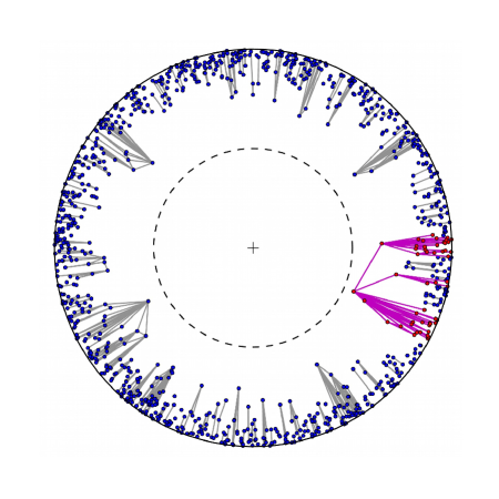
Figure 1: A realization of the subcritical hyperbolic graph $\mathrm{Poi}_{\alpha,\nu}(n)$ with parameters $\alpha=1.1$, $\nu=1$, $n=1000$. The outer circle of the figure corresponds to $B(O,R)$, the inner dashed circle is $B(O,R/2)$. The size of the largest connected component, in purple, is $|L_{1}|=51$.

The random hyperbolic model is defined as follows: for each $n\in\mathbb{N}$, we consider a Poisson point process on the disk $B_{h}(O,R)$ of the hyperbolic plane. The radius is equal to $R:=2\log(n/\nu)$ for some positive constant $\nu\in\mathbb{R}^{+}$ ($\log$ denotes here and throughout the paper the natural logarithm). The intensity function at polar coordinates $(r,\theta)$ for $0\leq r<R$ and $0\leq\theta<2\pi$ is

$$g(r,\theta):=\nu e^{\frac{R}{2}}f(r,\theta)$$

where $f(r,\theta)$ is the density function corresponding to the uniform probability on the disk $B_{h}(O,R)$ of the hyperbolic space of curvature $-\alpha^{2}$, that is $\theta$ is chosen uniformly at random in the interval $[0,2\pi)$ and independently of $r$ which is chosen according to the density function

$$f(r) :=\begin{cases}\displaystyle\frac{\alpha\sinh(\alpha r)}{\cosh(\alpha R)-1},&\text{if $0\leq r<R$},\\ 0,&\text{otherwise}.\end{cases}$$

Make then the following graph $G=(V,E)$. The set of vertices $V$ is the points set of the Poisson process and for $u,u^{\prime}\in V$, $u\neq u^{\prime}$, there is an edge with endpoints $u$ and $u^{\prime}$ provided the distance (in the hyperbolic plane) between $u$ and $u^{\prime}$ is at most $R$, i.e., the hyperbolic distance $\mathrm{d_{h}}(u,u^{\prime})$ between $u$ and $u^{\prime}$ is such that $\mathrm{d_{h}}(u,u^{\prime})\leq R$, where $\mathrm{d_{h}}(u,u^{\prime})$ is obtained by solving Equation (1)

For a given $n\in\mathbb{N}$, we denote this model by $\mathrm{Poi}_{\alpha,\nu}(n)$. Note in particular that

$$\int g(r,\theta)d\theta dr=\nu e^{\frac{R}{2}}=n,$$

and thus $\mathbb{E}|{V}|=n$. In the original model of Krioukov et al. [KPK⁺10], $n$ points, corresponding to vertices, are chosen uniformly and independently in the disk $B_{h}(O,R)$ of the hyperbolic space of curvature $-\alpha^{2}$, but since from a probabilistic point of view it is arguably more natural to consider the Poissonized version of this model, we consider the latter one; see also [GPP12] for the construction of the uniform model.

The restriction $\alpha>\frac{1}{2}$ and the role of $R$ guarantee that the resulting graph has bounded average degree (depending on $\alpha$ and $\nu$ only). If $\alpha<\frac{1}{2}$, then the degree sequence is so heavy tailed that this is impossible (the graph is with high probability connected in this case, as shown in [BFM16]). Moreover, if $\alpha>1$, then as the number of vertices grows, the largest component of a random hyperbolic graph has sublinear order (see  [BFM15, Theorem 1.4]).

Notations: We say that an event holds asymptotically almost surely (a.a.s.), if it holds with probability tending to $1$ as $n\to\infty.$ Given positive sequences $(a_{n})_{n\geq 1}$ and $(b_{n})_{n\geq 1}$ taking values in $\mathbb{R}$, we write $a_{n}=o(b_{n})$ to mean that $a_{n}/b_{n}\to 0$ as $n\to\infty$. Also we write $a_{n}=\Theta(b_{n})$ if $|a_{n}|/|b_{n}|$ is bounded away from 0 and $\infty$, and $a_{n}=\Omega(b_{n})$ if $|a_{n}|/|b_{n}|$ is bounded away from $0$.

Result: In this paper we study the size of the largest component of the graph in the case $\alpha>1$. In [BFM15, Theorem 1.4] it was shown that its size is a.a.s. at most $n^{1/\alpha+o(1)}$. The main result of this paper is the following improvement, finding the exact exponent:

Theorem 1.

Let $\alpha>1$ and $\nu\in\mathbb{R}^{+}$. Let $G=(V,E)$ be chosen according to $\mathrm{Poi}_{\alpha,\nu}(n)$, and let $L_{1}\subseteq G$ be the largest connected component of $G$. There is a constant $C>0$, such that, a.a.s., the following holds:

$$n^{\frac{1}{2\alpha}}(\log n)^{-C}\leq|L_{1}|\leq n^{\frac{1}{2\alpha}}(\log n)^{C}\ .$$

Remark 2.

A careful inspection of the proofs shows that all results hold with probability at least $1-o(n^{-1/2})$, and hence a Depoissonization argument (see [Pen03] for details) shows that Theorem 1 also holds for the original uniform model.

Related work: The size of the largest component in random hyperbolic graphs was first studied in [BFM15]: it was shown that for $\alpha>1$ it is at most $n^{1/\alpha+o(1)}$, whereas for $\alpha<1$ the largest component is linear. In the same paper the authors also showed that for $\alpha=1$ and $\nu$ sufficiently small there is a.a.s. no linear size component, whereas for $\alpha=1$ and $\nu$ sufficiently large a.a.s. there is a linear size component. In [FM18] the picture was made more precise: for $\alpha=1$ there is a critical intensity such that a.a.s. a linear size component exists iff $\nu$ is above a certain threshold. Also, for $\alpha<1$, for fixed $\alpha$ the size of the largest component is increasing in $\nu$, and for fixed $\nu$, it is decreasing in $\alpha$. Furthermore, in [BFM16] it was shown that for $\alpha<1/2$ the graph is connected a.a.s., whereas for $\alpha=1/2$ the probability of being connected tends to $1$ if $\nu\geq\pi$, and the probability of being connected is otherwise a monotone increasing function in $\nu$ that tends to $0$ as $\nu$ tends to $0$. For the case $1/2<\alpha<1$, it was shown in [KM19] that a.a.s. the second component is of size $\Theta((\log n)^{1/(1-\alpha)})$, whereas for $\alpha=1/2$ and $\nu$ sufficiently small it is $\Theta(\log n)$ with constant probability, and for $\alpha=1$ it is a.a.s. $\Omega(n^{b})$ for some $b>0$. Starting with the seminal work of [KPK⁺10], further aspects of random hyperbolic graphs have been discussed since then: the power law degree distribution, mean degree and clustering coefficient were analyzed in [GPP12]; the diameter was computed in [FK15, KM15, MS19], the spectral gap was analyzed in [KM18], typical distances were calculated in [ABF17], and bootstrap percolation in such graphs was considered in [CF16]. First passage percolation of random hyperbolic graphs (or more generally, geometric inhomogeneous random graphs) was analyzed in [KL].

Organization of the paper: In Section 2 we recall some well known properties of the random hyperbolic graph. Section 3 then describes the construction of the main tool of our proof: the separation zones. The existence of these zones shows that there is no long path of vertices with all vertices having roughly the same radial coordinates. Finally, in Section 4 we use the separation zones to control the size of the connected components of the graph which leads to the result of Theorem 1.

2 Preliminaries

From now on, we suppose $\alpha>1$. In this section we collect some properties concerning random hyperbolic graphs. For notational convenience, for any point $v=(r_{v},\theta_{v})$ of the ball $B(O,R)$ we define $t_{v}=R-R_{v}$, the radial distance to the boundary circle of radius $R$ (instead of the distance to the origin $O$), and we identify a vertex $v$ of the graph $G$ with the coordinate pair $v=(t_{v},\theta_{v})$. Moreover, we suppose throughout the paper that $R$ is an integer.

By the hyperbolic law of cosines (1), the hyperbolic triangle formed by the geodesics between points $p^{\prime}$, $p^{\prime\prime}$, and $p$, with opposing side segments of length $\mathrm{d^{\prime}_{h}}$, $\mathrm{d^{\prime\prime}_{h}}$, and $\mathrm{d_{h}}$ respectively, is such that the angle formed at $p$ is:

$$\theta_{\mathrm{d_{h}}}(\mathrm{d^{\prime}_{h}},\mathrm{d^{\prime\prime}_{h}})=\arccos\Big{(}\frac{\cosh\mathrm{d^{\prime}_{h}}\cosh\mathrm{d^{\prime\prime}_{h}}-\cosh\mathrm{d_{h}}}{\sinh\mathrm{d^{\prime}_{h}}\sinh\mathrm{d^{\prime\prime}_{h}}}\Big{)}.$$

Clearly, $\theta_{\mathrm{d_{h}}}(\mathrm{d^{\prime}_{h}},\mathrm{d^{\prime\prime}_{h}})=\theta_{\mathrm{d_{h}}}(\mathrm{d^{\prime\prime}_{h}},\mathrm{d^{\prime}_{h}})$. We state a very handy approximation for $\theta_{R}(\cdot,\cdot)$.

Lemma 3 ([GPP12, Lemma 3.1]).

If $0\leq\min\{\mathrm{d^{\prime}_{h}},\mathrm{d^{\prime\prime}_{h}}\}\leq R\leq\mathrm{d^{\prime}_{h}}+\mathrm{d^{\prime\prime}_{h}}$, then

$$\theta_{R}(\mathrm{d^{\prime}_{h}},\mathrm{d^{\prime\prime}_{h}})=2e^{\frac{1}{2}(R-\mathrm{d^{\prime}_{h}}-\mathrm{d^{\prime\prime}_{h}})}\big{(}1+\Theta(e^{R-\mathrm{d^{\prime}_{h}}-\mathrm{d^{\prime\prime}_{h}}})\big{)}.$$

A direct consequence of this lemma is the following corollary:

Corollary 4.

For any $R>0$, there is a function

$$\theta^{R}:\begin{array}[]{ccl}[0,R/2]^{2}&\to&\mathbb{R}^{+}\\ (t_{1},t_{2})&\mapsto&\theta^{R}\left(t_{1},t_{2}\right)\end{array}$$

such that

• $\theta^{R}\left(t_{1},t_{2}\right)=2e^{-\frac{1}{2}(R-t_{1}-t_{2})}\big{(}1+\Theta(e^{-\frac{1}{2}(R-t_{1}-t_{2})})\big{)}$

• two vertices $u,v\in V$ such that $t_{u}+t_{v}\leq R$ are connected by an edge iff $|\theta_{u}-\theta_{v}|\leq\theta^{R}\left(t_{u},t_{v}\right).$

Throughout, we will need estimates for measures of regions of the hyperbolic plane, and more specifically, for regions obtained by performing some set algebra involving a few balls. For a point $p$ of the hyperbolic plane $\mathbb{H}^{2}$, the ball of radius $\rho$ centered at $p$ will be denoted by $B_{p}(\rho)$, i.e., $B_{p}(\rho):=\{q\in\mathbb{H}^{2}:\mathrm{d_{h}}(p,q)\leq\rho\}$.

Also, we denote by $\mu(S)$ the measure of a set $S\subseteq\mathbb{H}^{2}$, i.e., $\displaystyle\mu(S):=\int_{S}f(r,\theta)drd\theta$.

Next, we collect a few standard results for such measures.

Lemma 5 ([GPP12, Lemma 3.2]).

If $0\leq\rho<R$, then $\mu(B_{O}(\rho))=\nu e^{-\alpha(R-\rho)}(1+o(1))$.

We also use classical Chernoff concentration bounds for Poisson random variables. See for instance ([BLM13] page 23).

Lemma 6 (Chernoff bounds).

If $X\sim\mathcal{P}(\lambda)$, then for any $x>0$,

$$\mathbf{P}\left(\left.X\geq\lambda+x\right.\right) \leq e^{-\frac{x^{2}}{2(\lambda+x)}}\quad\text{ and }\quad\mathbf{P}\left(\left.X\leq\lambda-x\right.\right)\leq e^{-\frac{x^{2}}{2(\lambda+x)}}.$$

In particular, for $x\geq\lambda$,

$$\mathbf{P}\left(\left.X\geq 2x\right.\right) \leq e^{-\frac{x}{4}}$$

Lemma 6 together with Lemma 3.2 of [GPP12] yield the following lemma:

Lemma 7.

Let $V$ be the vertex set of a graph chosen according to $\mathrm{Poi}_{\alpha,\nu}(n)$, and let $v$ be a vertex with $t_{v}>C\log R$ for $C$ sufficiently large. Then, a.a.s. ${|V\cap B_{v}(R)|}=\Theta(e^{\frac{1}{2}t_{v}})$.

3 Construction of the separation zones

In this section we explain how to construct the separation zones. We first define the following sectors

$$S(\theta_{1},\theta_{2})=\left\{\left.(t,\theta)\mid 0\leq t<R\text{ and }\theta_{1}\leq\theta<\theta_{2}\right.\right\}$$

and the annuli

$$\mathcal{L}(t^{-},t^{+})=\left\{\left.(t,\theta)\mid t^{-}\leq t<t^{+}\text{ and }0\leq\theta<2\pi\right.\right\}.$$

The following observation is a simple consequence of Lemma 5:

Observation 8.

For any $0\leq t^{-}<t^{+}<R/2$

$$\mathbf{E}\left[\left.|V\cap\mathcal{L}(t^{-},t^{+})|\right.\right]=\nu e^{\frac{R}{2}-\alpha t^{-}}(1-e^{-\alpha(t^{+}-t^{-})}+o(1)).$$

We then construct for each coordinate pair $(t_{0},\theta_{0})\in(0,R/2)\times[0,2\pi)$, a zone that separates points to the left from points to the right in $\left\{\left.(t,\theta),t\leq t_{0}\right.\right\}$. Precisely, define for $t_{0}<R/2$ and $\theta_{0}\in[0,2\pi)$, the following separation zone:

$$\mathcal{A}(t_{0},\theta_{0})=\left\{\left.(t,\theta)\mid t\leq t_{0}\text{ and }|\theta-\theta_{0}|\leq\theta^{R}\left(t,t\right)\right.\right\}.$$

We thus have the following observation:

Observation 9.

Suppose $V\cap\mathcal{A}(t_{0},\theta_{0})=\emptyset$. Let $v,w\in\left\{\left.(s,\theta),s\leq t_{0}\right.\right\}$ with $\theta_{v}<\theta_{0}<\theta_{w}$. Then $|\theta_{v}-\theta_{w}|>\theta^{R}(t_{v},t_{w})$, i.e. $v$ and $w$ are not connected by an edge.

Proof.

The function $\theta^{R}(t_{v},t_{w})$ is increasing in both of its arguments, hence we may assume that $t_{v}=t_{w}=t$. For this choice of $t$, $v$ and $w$ are connected by Corollary 4 iff $|\theta_{v}-\theta_{w}|\leq\theta^{R}(t,t)$. However, since $\mathcal{A}(t_{0},\theta_{0})=\emptyset$ and $\theta_{v}<\theta_{0}<\theta_{w}$, we have $|\theta_{v}-\theta_{w}|>2\theta^{R}(t,t)$, i.e. $v$ and $w$ are not connected by an edge. ∎

Figure 2: a separation zone

To use the previous observation, we need separation zones which do not contain any vertices. We prove below that this happens with large probability.

Lemma 10.

For any $K>0$, there is a constant $c>0$ which depends only on $\alpha$ and $\nu$ such that for any $t<R/2$,

$$\mathbf{P}\left(\left.\exists j\in\left\{\left.0,\dots,cR\right.\right\},V\cap\mathcal{A}(t,2j\theta^{R}\left(t,t\right))=\emptyset\right.\right)\geq 1-e^{-KR}\ .$$

Proof.

Consider the event

$$E=\left\{\left.\exists j\in\left\{\left.0,\dots,N\right.\right\},V\cap\mathcal{A}(t,2j\theta^{R}\left(t,t\right))=\emptyset\right.\right\}$$

for some $N$ that we will choose below. We recall that the set $\mathcal{A}(t,2j\theta^{R}\left(t,t\right))$ is included in the sector

$$S((2j-1)\theta^{R}\left(t,t\right),(2j+1)\theta^{R}\left(t,t\right)).$$

For different values of $j$, these sectors are disjoint, and thus the random variables $|V\cap\mathcal{A}(t,2j\theta^{R}\left(t,t\right))|$ are independent and

$$\mathbf{P}\left(\left.\overline{E}\right.\right)=\left(\left.\mathbf{P}\left(\left.|V\cap\mathcal{A}(t,0)|>0\right.\right)\right.\right)^{N+1}=\left(\left.1-e^{-\mathbf{E}\left[\left.|V\cap\mathcal{A}(t,0)|\right.\right]}\right.\right)^{N+1}$$

Then, as $t<R/2$, Corollaries 4 and 8 give

$$\mathbf{E}\left[\left.|V\cap\mathcal{A}(t,0)|\right.\right] \leq\sum_{1\leq i\leq\lceil t\rceil}2\theta^{R}\left(i,i\right)\mathbf{E}\left[\left.|V\cap\mathcal{L}(i-1,i)|\right.\right]$$

$$=\sum_{1\leq i\leq\lceil t\rceil}4e^{-\frac{R}{2}+i}\nu e^{R/2}e^{-\alpha(i-1)}(1-e^{-\alpha})(1+o(1))$$

$$=4\nu(e^{\alpha}-1)\sum_{1\leq i\leq\lceil t\rceil}e^{-(\alpha-1)i}(1+o(1))$$

$$\leq 4\nu\frac{(e^{\alpha}-1)e^{-(\alpha-1)}}{1-e^{-(\alpha-1)}}+o(1).$$

By choosing $N=cR$ for some constant $c>0$ sufficiently large (depending on $K$) the lemma follows. ∎

We will now consider layers starting from the boundary of $B_{O}(R)$: set

$$\forall i\geq 0,\ t_{i}=\left(\frac{4\alpha}{\alpha-1}+3i\right)\log R.$$

Let $t_{\max}=\frac{1}{2\alpha}R$ (note that $t_{\max}<R/2$), the distance to circle of radius $R$ roughly corresponding to the largest $t$ for which we can find an element of $V$ and set $i_{\max}=\min\left\{\left.i\geq 0,\ t_{i}\geq t_{\max}\right.\right\}$. We thus have

$$i_{\max}\leq R\text{ and }t_{\max}\leq t_{i_{\max}}\leq t_{\max}+3\log R.$$

We also set $t_{-1}=0$ and we define, for $i,j\in\left\{\left.0,\dots,i_{\max}\right.\right\}$, the angle

$$\theta_{i,j}=\theta^{R}\left(t_{i},t_{j}\right)$$

and the consecutive layers

$$\mathcal{L}_{i}=\mathcal{L}(t_{i-1},t_{i}).$$

Observation 11.

For any $i,j\in\left\{\left.0,\dots,i_{\max}\right.\right\}$,

$$\mathbf{E}\left[\left.|V\cap\mathcal{L}_{i}|\right.\right]=\nu e^{\frac{R}{2}-\alpha t_{i-1}}(1+o(1))\quad\text{and}\quad\theta_{i,j}=2e^{-\frac{1}{2}(R-t_{i}-t_{j})}\big{(}1+\Theta(e^{-\frac{1}{2}(R-t_{i}-t_{j})})\big{)}.$$

We now define the following separation zones: for every $i\in\left\{\left.0,\dots,i_{\max}\right.\right\}$, set $k_{\max}^{i}=\lceil 2\pi/(3cR\theta_{i,i})\rceil$ where $c$ is the constant given in Lemma 10 for $K=1$. For every $0\leq k<k_{\max}^{i}$, we find the $(k+1)$-th separation zone to be the closest (to the right) empty region to the angle $3cRk\theta_{i,i}$. More formally, define for $0\leq k<k^{i}_{\max}$,

$$j^{i,k} =\min\left\{\left.j\in\mathbb{N}\mid V\cap\mathcal{A}(t_{i},(3cRk+2j)\theta_{i,i})=\emptyset\right.\right\}.$$

We assign $\mathcal{A}^{i,k}$ then to be the closest region to $3cRk\theta_{i,i}$:

$$\mathcal{A}^{i,k} =\mathcal{A}(t_{i},(3cRk+2j^{i,k})\theta_{i,i}),$$

where $\min\emptyset=\infty$ and in this case $\mathcal{A}^{i,k}=\emptyset$. The set $\mathcal{A}^{i,k}$ represents the $(k+1)$-th separation zone of layer $i$. For notational convenience, we also set $\mathcal{A}^{i,k^{i}_{\max}}=\mathcal{A}^{i,0}$. We could have $\mathcal{A}^{i,k}=\mathcal{A}^{i,k+1}$, and the two sets might not even be well defined. We will thus use Lemma 10 to show that asymptotically almost surely none of the two things happens.

In order to state the next lemma properly, we define the following (pseudo)distance between separation zones:

$$\forall A,B\subset B_{O}(R),\ d(A,B)=\inf\left\{\left.|\theta-\theta^{\prime}|\ |\ (t,\theta)\in A,\ (t^{\prime},\theta^{\prime})\in B\right.\right\}.$$

Lemma 12.

Let $c$ be the constant given in Lemma 10 for $K=1$ (depending only on $\alpha$ and $\nu$). Then the event $\mathcal{E}_{R}$ defined by

$$\mathcal{E}_{R}=\left\{\left.\forall 0\leq i\leq i_{\max},\ \forall 0\leq k<k_{\max}^{i},\ \mathcal{A}^{i,k}\neq\emptyset\text{ and }cR\theta_{i,i}\leq d(\mathcal{A}^{i,k},\mathcal{A}^{i,k+1})\leq 5cR\theta_{i,i}\right.\right\}$$

occurs a.a.s.

Proof.

Let $c$ be the constant given in Lemma 10 for $K=1$ and consider the event

$$\mathcal{F}_{R}=\left\{\left.\forall 0\leq i\leq i_{\max},\ \forall 0\leq k<k_{\max}^{i},\ \exists j\in\left\{\left.0,\dots,cR\right.\right\},V\cap\mathcal{A}(t_{i},(3cRk+2j)\theta_{i,i})=\emptyset\right.\right\}.$$

Clearly, $\mathcal{F}_{R}\subset\mathcal{E}_{R}$ and it is sufficient to bound $\mathbf{P}\left(\left.\overline{\mathcal{F}_{R}}\right.\right)$. Then, for $R$ large enough, using the definition of $k_{\max}^{i}$,

$$\mathbf{P}\left(\left.\overline{\mathcal{F}_{R}}\right.\right)\leq \sum_{\begin{subarray}{c}0\leq i\leq i_{\max}\\ 0\leq k<k_{\max}^{i}\end{subarray}}\mathbf{P}\left(\left.\forall j\in\left\{\left.0,\dots,cR\right.\right\},V\cap\mathcal{A}(t_{i},(3cRk+2j)\theta_{i,i})\neq\emptyset\right.\right)$$

$$= \sum_{0\leq i\leq i_{\max}}k_{\max}^{i}\mathbf{P}\left(\left.\forall j\in\left\{\left.0,\dots,cR\right.\right\},V\cap\mathcal{A}(t_{i},2j\theta_{i,i})\neq\emptyset\right.\right)$$

$$\leq C_{1}\sum_{0\leq i\leq i_{\max}}e^{\frac{R}{2}-t_{i}}e^{-R}\leq C_{2}e^{-\frac{1}{2}R}.$$

Since the last quantity goes to zero as $R$ tends to infinity, the lemma is proven. ∎

Figure 3: The separation zones

Hence, a.a.s. the distance between two consecutive separation zones $\mathcal{A}^{i,k}$ and $\mathcal{A}^{i,k+1}$ is always of the order $R\theta_{i,i}$. Define now, on $\mathcal{E}_{R}$, the area $\mathcal{B}_{i,k}$ between two separation zones: for $1\leq k<k^{i}_{\max}$,

$$\mathcal{B}_{i,k}=\left\{\left.(t,\theta)\in B_{O}(R)\mid t\leq t_{i}\text{ and }\forall(t,\theta_{-})\in\mathcal{A}^{i,k-1},\ \theta>\theta_{-}\ \text{ and }\ \forall(t,\theta_{+})\in\mathcal{A}^{i,k},\ \theta<\theta_{+}\right.\right\}$$

and

$$\mathcal{B}_{i,0}=\left\{\left.(t,\theta)\in B_{O}(R)\mid t\leq t_{i}\text{ and }\forall(t,\theta_{-})\in\mathcal{A}^{i,k^{i}_{\max}-1},\ \theta>\theta_{-}\ \text{ or }\ \forall(t,\theta_{+})\in\mathcal{A}^{i,0},\ \theta<\theta_{+}\right.\right\}$$

We point out that every path of connected points from $u\in V\cap\mathcal{B}_{i,k}$ to $v\in V\cap\mathcal{B}_{i,\ell}$ with $k\neq\ell$ has to go through a vertex $w\in V$ such that $t_{w}>t_{i}$, i.e. points cannot be connected ”below” as described in Figure 4. More formally, rewriting Observation 9 we obtain the following observation.

Observation 13.

Suppose $\mathcal{A}^{i,k}=\emptyset$. Let $u\in V\cap\mathcal{B}_{i,k}$ to $v\in V\cap\mathcal{B}_{i,\ell}$ with $k\neq\ell$. Then $u$ and $v$ can only be connected by a path that has at least one intermediate vertex $w\in V$ such that $t_{w}>t_{i}$.

Proof.

Note that $t_{u},t_{v}\leq t_{i}$. Then by Observation 9, $u$ and $v$ are not connected by an edge. Since this holds for any $k\neq\ell$ and any $u,v$, there can be no path between $u$ and $v$ containing vertices $w\in V$ such that $t_{w}\leq t_{i}$ (see also Figure 4). ∎

Figure 4: The green points are connected while the red ones are not.

4 Covering component

On a high level, the advantage of separation zones is that it is impossible to stay in the same connected component going from right to left (or the other direction) remaining always at the same radius or going towards the boundary. We will thus construct, starting from a certain vertex, a covering component, that is, a component which covers a.a.s. the whole connected component of the vertex if this vertex is the vertex closest to the center of its connected component.

We describe now in detail the iterative construction process of the covering component. Suppose that the event $\mathcal{E}_{R}$ holds. This happens a.a.s. according to Lemma 12. Consider a vertex $v\in V$. If $v$ is in the layer $\mathcal{L}_{0}$, we define $C_{v}=\left\{\left.v\right.\right\}$ and if $v\in\mathcal{L}_{i}$ for $0\leq j<i\leq i_{\max}$, we set

$$\Theta_{i,j}(v)=V\cap\mathcal{L}_{j}\cap S(\theta_{v}-2\theta_{i,j},\theta_{v}+2\theta_{i,j})$$

and (see also Figure 5)

$$C_{v} =\left\{\left.v\right.\right\}\cup\bigcup_{j=0}^{i-1}\bigcup_{u\in\Theta_{i,j}(v)}C_{u}.$$

Denote now by $k$ the unique integer such that $v\in\mathcal{L}_{i}\cap\mathcal{B}_{i,k}$. The covering component of $v$ is then defined as

$$\mathbf{C}_{v}=\bigcup_{u\in V\cap\mathcal{L}_{i}\cap\mathcal{B}_{i,k}}C_{u}.$$

Figure 5: Construction of $C_{v}$

We also denote by $Conn(v)$ the connected component of $v$. The following lemma shows that the covering component of $v$ indeed covers the connected component of $v$ if $v$ is the closest vertex of the center in this component.

Lemma 14.

A.a.s. for any $v\in B_{O}(R)$, if $t_{v}=\max\left\{\left.t_{u}\mid u\in Conn(v)\right.\right\}$ the connected component of $v$ is included in $\mathbf{C}_{v}$.

Proof.

Suppose that the event $\mathcal{E}_{R}$ holds. This happens a.a.s. according to Lemma 12.

By contradiction, consider a vertex $u$ in the connected component of $v$ that is not contained in $\mathbf{C}_{v}$, and a shortest path $v_{0}=v,\ldots,v_{m}=u$. Hence there exists a smallest $k\geq 1$ such that the vertex $v_{k}$ is not in $\mathbf{C}_{v}$. Let $\mathcal{L}_{i_{k}}$ be the layer of $v_{k}$.

Suppose now there exists $k^{\prime}<k$ so that for some $i_{k^{\prime}}>i_{k}$, $v_{k^{\prime}}\in\mathcal{L}_{i_{k^{\prime}}}$. We may then choose the largest $k^{\prime}$, so that

$$\forall\ell\in\left\{\left.k^{\prime}+1,\dots,k\right.\right\},\ \exists i_{\ell}\leq i_{k},\quad v_{\ell}\in\mathcal{L}_{i_{\ell}}\quad\text{(see Figure \ref{fig:concomp}).}$$

Figure 6: Explanation of the proof of Lemma 14

Hence, the $v_{\ell}$ are in the same zone $\mathcal{B}_{i_{k},s}$ as $v_{k}$ and

$$|\theta_{v_{k^{\prime}}}-\theta_{v_{k}}|\leq\theta_{i_{k^{\prime}}i_{k}}+5cR\theta_{i_{k}i_{k}}\leq 2\theta_{i_{k^{\prime}}i_{k}}$$

and thus $v_{k}\in C_{v_{k^{\prime}}}\subset\mathbf{C}_{v}$ which is impossible. Thus necessarily $v=v_{0}$ is in the same layer as $v_{k}$ or in a layer closer to the boundary. Since $v$ is by hypothesis the vertex such that $t_{v}=\max\left\{\left.t_{u}\mid u\in Conn(v)\right.\right\}$, we must have $v\in\mathcal{L}_{i_{k}}$. Therefore, by Observation 13, $v$ and $v_{k}$ must be in the same zone $\mathcal{B}_{i_{k},s}$ for some $s$ and thus $v_{k}\in\mathbf{C}_{v}$. ∎

Lemma 15.

A.a.s.,

$$\forall 0\leq j<i\leq i_{\max},\ \forall v\in\mathcal{L}_{i},\ |\Theta_{i,j}(v)|\leq 4\max(8R,\mathbf{E}\left[\left.|\Theta_{i,j}(t_{i},0)|\right.\right])$$

Proof.

Let $d_{i,j}=2\max(8R,\mathbf{E}\left[\left.|\Theta_{i,j}(t_{i},0)|\right.\right])$. For each $0\leq j<i\leq i_{\max}$, divide layer $\mathcal{L}_{j}$ into $\lceil\pi/(2\theta_{i,j})\rceil$ sectors of angle (at most) $4\theta_{i,j}$. For any such sector $S_{k}^{(i,j)}$, for any $0\leq j<i\leq i_{\max}$, from Lemma 6 we have

$$\mathbf{P}\left(\left.|S_{k}^{(i,j)}\cap V\cap\mathcal{L}_{j}|>d_{i,j}\right.\right)\leq e^{-2R}.$$

By a union bound over all $\lceil\pi/(2\theta_{i,j})\rceil$ sectors $S_{k}^{(i,j)}$ and then over all $i,j$, we have

$$\mathbf{P}\left(\left.\exists 0\leq j<i\leq i_{\max},\exists 1\leq k\leq\lceil\pi/(2\theta_{i,j})\rceil,\ |S_{k}^{(i,j)}\cap V\cap\mathcal{L}_{j}|>d_{i,j}\right.\right)\leq R^{2}e^{R/2}e^{-2R}=o(1).$$

Hence, since for each vertex $v\in V\cap\mathcal{L}_{i}$, the set $\Theta_{i,j}(v)$ can intersect at most two adjacent sectors $S_{k}^{(i,j)}$, we have

$$\mathbf{P}\left(\left.\exists 0\leq j<i\leq i_{\max},\ \exists v\in V\cap\mathcal{L}_{i},\ |\Theta_{i,j}(v)|>2d_{i,j}\right.\right)=o(1).$$

∎

Lemma 16.

There is a constant $K\geq 1$ such that a.a.s.

$$\forall 0\leq i\leq i_{\max},\ \forall v\in\mathcal{L}_{i},\ |\mathbf{C}_{v}|\leq e^{2t_{0}+\frac{1}{2}t_{i}}.$$

Proof.

We first give an upper bound for $|C_{v}|$: recall first that Lemma 15 says that the event

$$\mathcal{A}=\left\{\left.\forall 0\leq j<i\leq i_{\max},\ \forall v\in V\cap\mathcal{L}_{i},\ |\Theta_{i,j}(v)|\leq 4\max(8R,\mathbf{E}\left[\left.|\Theta_{i,j}(t_{i},0)|\right.\right])\right.\right\}$$

happens a.a.s. We now proceed by induction on $i$ and prove that, on $\mathcal{A}$, for any $0\leq i\leq i_{\max}$,

$$\forall j\leq i,\ \forall v\in V\cap\mathcal{L}_{j},\ |C_{v}|\leq Ke^{\frac{t_{0}+t_{i}}{2}}.$$

for the constant $K=37\nu$. As for any $v\in V\cap\mathcal{L}_{0}$, $C_{v}=\left\{\left.v\right.\right\}$, the result is obvious for $i=0$. Suppose now it is true for some $0\leq i<i_{\max}$. On the event $\mathcal{A}$, for any $v\in V\cap\mathcal{L}_{i+1}$,

$$|C_{v}| \leq 1+\sum_{0\leq j\leq i}\sum_{u\in\Theta_{i+1,j}(v)}|C_{u}|\leq 1+|\Theta_{i+1,0}(v)|+\sum_{1\leq j\leq i}\sum_{u\in\Theta_{i+1,j}(v)}|C_{u}|$$

$$\leq 1+4\max(8R,\mathbf{E}\left[\left.|\Theta_{i+1,0}(t_{i+1},0)|\right.\right])+\sum_{1\leq j\leq i}4\max(8R,\mathbf{E}\left[\left.|\Theta_{i+1,j}(t_{i+1},0)|\right.\right])19\nu e^{\frac{t_{0}+t_{j}}{2}}.$$

According to Observation 11, if $R$ is large enough, for $j=0$,

$$\mathbf{E}\left[\left.|\Theta_{i+1,0}(t_{i+1},0)|\right.\right] =4\theta_{i+1,0}\mathbf{E}\left[\left.|V\cap L_{0}|\right.\right]\leq 9\nu e^{R/2-\frac{1}{2}(R-t_{i+1}-t_{0})}=9\nu e^{\frac{t_{0}+t_{i+1}}{2}},$$

and for $j\geq 1$,

$$\mathbf{E}\left[\left.|\Theta_{i+1,j}(t_{i+1},0)|\right.\right] =4\theta_{i+1,j}\mathbf{E}\left[\left.|V\cap L_{j}|\right.\right]\leq 9\nu e^{R/2-\alpha t_{j-1}-\frac{1}{2}(R-t_{i+1}-t_{j})}=9\nu e^{\frac{t_{j}+t_{i+1}}{2}-\alpha t_{j-1}}.$$

Recall that $t_{-1}=0$ and for $i\geq 0$, $t_{i}=(\frac{4\alpha}{\alpha-1}+3i)\log R$. This leads to the following bound for $|C_{v}|$ for large $R$:

$$|C_{v}| \leq 1+36\nu e^{\frac{t_{0}+t_{i+1}}{2}}+32RK\sum_{1\leq j\leq i}e^{\frac{t_{0}+t_{j}}{2}}+36K\nu^{2}e^{\frac{t_{0}+t_{i+1}}{2}}\sum_{1\leq j\leq i}e^{-\alpha t_{j-1}+t_{j}}$$

$$\leq 1+36\nu e^{\frac{t_{0}+t_{i+1}}{2}}\left(1+\frac{K}{\nu}R^{1/2}+\nu^{2}KR^{-\alpha}\right)\leq 37\nu e^{\frac{t_{0}+t_{i+1}}{2}}$$

Now we can proceed to obtain an upper bound for $|\mathbf{C}_{v}|$: For $i\in\left\{\left.0,\dots,i_{\max}\right.\right\}$, denote by $\Gamma_{i}$ the set

$$\Gamma_{i}=\left\{\left.v\in V\cap\mathcal{L}_{i}\Bigm{|}|\theta_{v}|\leq 5cR\theta_{i,i}\right.\right\}.$$

According to Observation 11, there is a constant $K$ depending only on $\nu$ such that for $R$ large enough and $i\in\left\{\left.0,\dots,i_{\max}\right.\right\}$,

$$\mathbf{E}\left[\left.|\Gamma_{i}|\right.\right] =10cR\theta_{i,i}\mathbf{E}\left[\left.|V\cap\mathcal{L}_{i}|\right.\right]\leq KRe^{-\frac{1}{2}(R-2t_{i})}e^{\frac{R}{2}-\alpha t_{i-1}}=KRe^{t_{i}-t_{i-1}-(\alpha-1)t_{i-1}}\leq KRe^{t_{0}}\leq\frac{1}{2}e^{\frac{3}{2}t_{0}}.$$

Therefore,

$$\mathbf{P}\left(\left.\mathcal{E}_{R}\cap\left\{\left.\exists i\in\left\{\left.0,\dots,i_{\max}\right.\right\},\ \exists k\in\left\{\left.1,\dots,k^{i}_{\max}\right.\right\},|V\cap\mathcal{L}_{i}\cap\mathcal{B}_{i,k}|\geq e^{\frac{3}{2}t_{0}}\right.\right\}\right.\right)$$

$$\leq\sum_{i=0}^{i_{\max}}\left\lceil\frac{1}{2cR\theta_{i,i}}\right\rceil\mathbf{P}\left(\left.|\Gamma_{i}|\geq e^{\frac{3}{2}t_{0}}\right.\right)$$

Now, since $|\Gamma_{i}|$ is a Poisson variable, Lemma 6 says that

$$\mathbf{P}\left(\left.|\Gamma_{i}|\geq e^{\frac{3}{2}t_{0}}\right.\right)\leq e^{-e^{\frac{3}{2}t_{0}}/8}.$$

Thus, the previous probability is smaller than

$$\sum_{i=0}^{i_{\max}}\frac{1}{2cR}e^{\frac{R}{2}-t_{i}}e^{-e^{\frac{3}{2}t_{0}}/8}\leq e^{R/2-e^{\frac{3}{2}t_{0}}/8},$$

which tends to 0 as $R$ tends to infinity.

Finally, a.a.s., for any $i\geq 0$ and any $v\in V\cap\mathcal{L}_{i}$, the cardinality of $\mathbf{C}_{v}$ satisfies

$$|\mathbf{C}_{v}| \leq\max_{u\in V\cap\mathcal{L}_{i}}|C_{u}|\max_{k\leq k^{i}_{\max}}|V\cap\mathcal{L}_{i}\cap\mathcal{B}_{i,k}|\leq Ke^{\frac{t_{0}+t_{i}}{2}}e^{\frac{3}{2}t_{0}},$$

and the lemma follows. ∎

Proof of Theorem 1.

According to Lemma 16, there is a constant $K>0$ such that, a.a.s.

$$\max_{v\in V}|Conn(v)|\leq\max_{v\in V}|\mathbf{C}_{v}| \leq e^{2t_{0}+\frac{1}{2}t_{i_{\max}}}\leq e^{2t_{0}+\frac{t_{\max}+3\log R}{2}}=e^{\frac{R}{4\alpha}+\left(\frac{8\alpha}{\alpha-1}+\frac{3}{2}\right)\log R}.$$ (2)

By Lemma 14 we obtain the upper bound for $|L_{1}|$ in the theorem.

For the lower bound, by Lemma 5, for any function $\omega$ tending to infinity with $n$ arbitrarily slowly, $\mu(B_{O}(r_{\max}+\omega)\gg 1/n$, and hence a.a.s. we find a vertex $v$ with $t_{v}\geq t_{\max}-\omega$. In such case, the degree of $v$ is, by Lemma 7, a.a.s. $\Theta(e^{\frac{1}{2}(t_{\max}-\omega))})=n^{\frac{1}{2\alpha}+o(\omega/n)}$. The degree of a vertex is a lower bound on the size of its component, and hence Theorem 1 follows.

∎

References

- [ABF17] M. A. Abdullah, M. Bode, and N. Fountoulakis. Typical distances in a geometric model for complex networks. Internet Mathematics, 1, 2017.
- [BFM15] M. Bode, N. Fountoulakis, and T. Müller. On the largest component of a hyperbolic model of complex networks. Electronic J. of Combinatorics, 22(3):P3.24, 2015.
- [BFM16] M. Bode, N. Fountoulakis, and T. Müller. The probability of connectivity in a hyperbolic model of complex networks. Random Structures & Algorithms, 49(1):65–94, 2016.
- [BKL+17] K. Bringmann, R. Keusch, J. Lengler, Y. Maus, and A.R. Molla. Greedy routing and the algorithmic small-world phenomenon. In Proceedings of the ACM Symposium on Principles of Distributed Computing, PODC’17, pages 371–380, New York, NY, USA, 2017. ACM.
- [BLM13] S. Boucheron, G. Lugosi, and P. Massart. Concentration inequalities. Oxford University Press, Oxford, 2013. A nonasymptotic theory of independence, With a foreword by Michel Ledoux.
- [BnPK10] M. Boguñá, F. Papadopoulos, and D. Krioukov. Sustaining the internet with hyperbolic mapping. Nature Communications, 1:62, 2010.
- [CF16] E. Candellero and N. Fountoulakis. Clustering and the hyperbolic geometry of complex networks. Internet Mathematics, 12(1–2):2–53, 2016.
- [FK15] T. Friedrich and A. Krohmer. On the diameter of hyperbolic random graphs. In Automata, Languages, and Programming - 42nd International Colloquium – ICALP Part II, volume 9135 of LNCS, pages 614–625. Springer, 2015.
- [FM18] N. Fountoulakis and T. Müller. Law of large numbers for the largest component in a hyperbolic model of complex networks. Annals of Applied Probability, 28:607–650, 2018.
- [GPP12] L. Gugelmann, K. Panagiotou, and U. Peter. Random hyperbolic graphs: Degree sequence and clustering. In Automata, Languages, and Programming - 39th International Colloquium – ICALP Part II, volume 7392 of LNCS, pages 573–585. Springer, 2012.
- [KL] J. Komjathy and B. Lodewijks. Explosion in weighted hyperbolic random graphs and geometric inhomogeneous random graphs. Stochastic Processes and its Applications, to appear.
- [KM15] M. Kiwi and D. Mitsche. A bound for the diameter of random hyperbolic graphs. In Proceedings of the 12th Workshop on Analytic Algorithmics and Combinatorics – ANALCO, pages 26–39. SIAM, 2015.
- [KM18] M. Kiwi and D. Mitsche. Spectral gap of random hyperbolic graphs and related parameters. Annals of Applied Probability, 28:941–989, 2018.
- [KM19] M. Kiwi and D. Mitsche. On the second largest component of random hyperbolic graphs. SIAM Journal on Discrete Mathematics, 33(4):2200–2217, 2019.
- [KPK+10] D. Krioukov, F. Papadopoulos, M. Kitsak, A. Vahdat, and M. Boguñá. Hyperbolic geometry of complex networks. Phyical Review E, 82(3):036106, 2010.
- [MS19] T. Müller and M. Staps. The diameter of KPKVB random graphs. Advances of Applied Probability, 51(2):358–377, 2019.
- [Pen03] M. Penrose. Random geometric graphs. Oxford University Press, 2003.
- [TM67] J. Travers and S. Milgram. The small world problem. Psychology Today, 1(1):61–67, 1967.