Improved neutrino-nucleon interactions in dense and hot matter for numerical simulations

Abstract

Neutrinos play an important role in compact star astrophysics: neutrino-heating is one of the main ingredients in core-collapse supernovae, neutrino-matter interactions determine the composition of matter in binary neutron star mergers and have among others a strong impact on conditions for heavy element nucleosynthesis and neutron star cooling is dominated by neutrino emission except for very old stars. Many works in the last decades have shown that in dense matter medium effects considerably change the neutrino-matter interaction rates, whereas many astrophysical simulations use analytic approximations which are often far from reproducing more complete calculations. In this work we present a scheme which allows to incorporate improved rates for charged current interactions, into simulations and show as an example some results for core-collapse supernovae, where a noticeable difference is found in the location of the neutrinospheres of the low-energy neutrinos in the early post-bounce phase.

I Introduction

The first detection of gravitational waves (GWs) from a binary neutron star (BNS) merger by the LIGO-Virgo collaboration in August 2017, the event GW170817, in coincidence with the observation of a gamma ray burst (GRB170817a) and an electro-magnetic counterpart established the beginning of multi-messenger astronomy Abbott et al. (2017). Many additional detections are expected including several BNS mergers, during current and forthcoming campaigns by large interferometric gravitational wave detectors. This rapidly evolving new astronomy is revolutionizing the exploration of the universe by addressing fundamental questions such as the nature of gravity, of dark matter, the origin of elements heavier than iron and of properties of dense matter in compact stars. A complete understanding of these exciting observations will be achieved once they can be successfully confronted to the predictions of theoretical modeling for which still many questions remain open, among others concerning neutrino interactions. The latter play an essential role for astrophysics of compact objects:

1. The dynamics of BNS mergers only marginally depend on neutrino interactions. However, ejecta composition and nucleosynthesis conditions are very sensitive to the neutrino treatment and neutrino interactions.

2. The heating by neutrinos of the stalled shock wave represents a crucial element for the dynamics of core-collapse supernovae (CCSN), contributing to the explosion mechanism

3. (Proto)-neutron star cooling is dominated by neutrino emission for millions of years.

Simulations of these processes are very expensive, so that currently mostly analytic expressions for the relevant reaction rates Bruenn (1985); Rosswog and Liebendoerfer (2003); Burrows et al. (2006); Schmitt and Shternin (2018) are applied, which are, however, often based on very crude approximations. Several corrections have been added to the original expressions Bruenn (1985), such as weak magnetism and recoil Horowitz (2002), nuclear structure corrections Horowitz (1997); Bruenn and Mezzacappa (1997), effective masses and chemical potentials for nucleons in dense matter Reddy et al. (1998); Roberts et al. (2012); Martinez-Pinedo et al. (2012), additional reactions Hannestad and Raffelt (1998); Fischer et al. (2020) and superfluidity in cooling neutron stars older than several minutes Yakovlev et al. (2001). Several authors have, however, pointed out since decades that in dense matter different effects can additionally modify the neutrino matter interaction rates and neutrino emissivities by orders of magnitude, in particular nuclear correlations Burrows and Sawyer (1998, 1999); Reddy et al. (1999); Navarro et al. (1999); Margueron et al. (2004); Horowitz and Schwenk (2006); Horowitz et al. (2017). (Special) relativistic effects can play an important role, too Leinson and Perez (2001); Leinson (2002); Roberts and Reddy (2017). Most of the above discussed modifications have been cast into correction factors to the original analytic expressions for practical use in simulations. The NuLib library by Evan O’Connor O’Connor (2015) provides the corresponding neutrino opacities.

It is, however, not possible to provide analytic expressions taking into account all known corrections. In view of the computational effort, only few simulations go indeed beyond the analytical expressions. In particular, the full phase space has been considered in several PNS cooling simulations Pons et al. (1999); Roberts et al. (2012) as well as for charged-current opacities in the spherically symmetric CCSN simulations of Fischer et al. (2020) and the Garching group has implemented additionally nuclear correlations following the simplified formalism of Burrows and Sawyer (1998, 1999), see Buras et al. (2006); Hüdepohl et al. (2010). However, as for neutrino-nucleus reactions, where already for a long time tabulated and accurate data on selected nuclei from microscopic calculations accounting for nuclear correlations and thermal effects exist Fuller et al. (1982); Langanke and Martinez-Pinedo (2001, 2003); Oda et al. (1994); Pruet and Fuller (2003); Juodagalvis et al. (2010), it is desirable that improved rates for neutrino-nucleon reactions become more generally available. In Roberts and Reddy (2017) a first step has been performed in this direction, neutrino opacities for charged current reactions with the full relativistic phase space including mean field corrections are provided via the nuOpac library. In the present work we perform a step further towards a complete neutrino toolkit, allowing to provide state-of-the-art neutrino-matter interaction rates directly applicable to simulations. As Roberts and Reddy (2017), we will concentrate on charged current neutrino-nucleon interactions, i.e. neutrino absorption and creation. We will stick to non-relativistic kinematics, but in addition to the full phase space, which is important at high densities Roberts and Reddy (2017); Fischer et al. (2020), we will include nuclear correlations via the so-called “Random Phase Approximation”(RPA). The impact of RPA correlations on neutrino opacities has been studied in several works, see e.g. Refs. Reddy et al. (1999); Burrows and Sawyer (1999), but mostly only grey, i.e. neutrino energy independent, correction factors to the above cited analytic approximation have yet been implemented. As discussed in Section II.3, the importance of RPA correlations is, however, energy dependent and a density and temperature dependent shift in reaction thresholds is induced. It is thus obvious that the full physics cannot be included into a grey factor and we will for the first time provide opacities with the full dependence on neutrino energy $E_{\nu}$, baryon number density $n_{B}$, temperature $T$ and electron fraction $Y_{e}$.

We will consider thermodynamic conditions relevant for BNS mergers, CCSN and (proto)-neutron star cooling during the first minutes which are rather similar: hot and dense nuclear matter with different asymmetries, i.e. proton to neutron ratios. In the central and hot parts, matter is homogeneous, whereas in the outer regions, containing more dilute and cold matter, nuclear clusters coexist with free nucleons. Charged current neutrino-nucleon reactions thereby, together with neutrino-nucleon scattering, not only control neutrino diffusion and emission in the central part, but strongly influence the physics close to the neutrinospheres, too, which is important for the dynamics and the characteristics of the emerging neutrinos. Charged current reactions on nucleons contribute critically to the heating of matter behind the shock in a CCSN, too.

Since the aim of our work is to provide results for the interaction rates going beyond the analytic approximations, complete opacity data as function of $E_{\nu},n_{B},T$ and $Y_{e}$ as calculated within the present work can be found in tabular form on the Compose data base Typel et al. (2015) together with the underlying equation of state (EoS) data. It has been emphasized many times that it is important to determine neutrino-nucleon interactions coherently with the underlying EoS, i.e. employing the same model for nuclear interactions, see e.g. Reddy et al. (1999). In contrast to Roberts and Reddy (2017) who provide routines and Fischer et al. (2020) who use a phase space integration “on the fly” during spherically symmetric simulations, we have chosen to directly provide opacity tables since the numerical calculations to obtain the rates in RPA (and probably any other scheme taking into account nuclear correlations) are much more time consuming than the simpler phase space integrations due to the existence of collective excitations in the nuclear response, see e.g. Hernandez et al. (1999). They have thus anyway to be tabulated before they can be implemented into simulations. We will show that our scheme can indeed be applied to simulations and perform CCSN simulations with fully energy dependent RPA correlations. The impact on the early post bounce evolution is discussed.

The paper is organized as follows. In Section II, neutrino opacities from charged current neutrino-nucleon interactions are computed. After briefly recalling the formalism in Sec. II.1, we compute in Sec. II.2 the polarization function within different approximations devised in previous works, some of them going beyond the standard (elastic) one. Results concerning neutrino opacities in these different approximations are given in Sec. II.3. Section III shows some outputs from CCSN simulations using these neutrino opacities in the solution of neutrino transport. All these points are summarized and discussed in Section IV.

II Charged current neutrino opacities

As mentioned in the introduction, different approximations have been considered to derive neutrino opacities from charged current neutrino-nucleon interactions. The elastic approximation Bruenn (1985) consists in neglecting any momentum transfer to the nucleons, assuming non-interacting nucleons and approximating the nucleonic form factors by lowest order constants. In Horowitz (2002), several corrections are introduced and corresponding analytic expressions are derived: (i) a momentum dependence of the nucleonic form factors which becomes important for energies close to the relevant scale of 1 GeV and which can thus safely be neglected in our case, (ii) weak magnetism corrections to the nucleonic form factors which are proportional to the difference in proton and neutron magnetic moment. These corrections are relevant at any density and can be of the order of 10%, (iii) phase space corrections up to order $E_{\nu}/m_{i}$, where $m_{i}$ are free nucleon masses and $E_{\nu}$ the neutrino energy.

The seminal work of Refs. Reddy et al. (1998, 1999); Burrows and Sawyer (1999) in the late 1990’s discusses the effect of nuclear interactions on the opacities as well in mean field approximation as in RPA. The latter is a method widely used in nuclear physics in order to account for nuclear correlations beyond mean field. It sums up particle-hole excitations of the nuclear medium within the long range collective (linear) response. At low densities, mean field is recovered. RPA correlations can reduce opacities by up to a factor five in high density matter Reddy et al. (1999); Burrows and Sawyer (1999); Dzhioev and Martínez-Pinedo (2018).

More recently, interactions in dense asymmetric matter have regained interest since it has been pointed out that they lead to a difference in proton and neutron single particle energies which can be of the order of several tens of MeV and can have sizable consequences for charged current opacities. Several authors have investigated the impact of these interactions by introducing effective masses and chemical potentials calculated from mean field into the elastic approximation opacity on proto-neutron star cooling Roberts et al. (2012); Martinez-Pinedo et al. (2012). Since the effect is opposite for neutrinos and anti-neutrinos, the energy difference between neutrinos and anti-neutrinos during a CCSN is enhanced, allowing for more neutron rich ejecta in CCSN neutrino driven winds with consequences for nucleosynthesis Roberts et al. (2012); Martinez-Pinedo et al. (2012). Roberts and Reddy (2017) have incorporated these mean field effects within full relativistic kinematics and have shown that in particular at high densities, when the transferred momentum becomes large, opacities are altered by a factor of a few.

In the following section II.1 we will present the general formalism before deriving explicit expressions within different approximations and discussing numerical results.

II.1 Formalism

In this section we will derive expressions for neutrino opacities arising from the following reactions for neutrino

$$p+e^{-}\leftrightarrow n+\nu_{e}\quad\quad p\leftrightarrow n+e^{+}+\nu_{e}$$ (1)

and anti-neutrino opacities

$$n\leftrightarrow p+e^{-}+\bar{\nu}_{e}\quad\quad n+e^{+}\leftrightarrow p+\bar{\nu}_{e}$$ (2)

following Refs. Sedrakian and Dieperink (1999); Schmitt et al. (2006). Let us consider a general process (creation/absorption) with an incoming/outgoing nucleon and an incoming/outgoing lepton, where one of the leptons is a neutrino. The different reaction rates can be calculated from the kinetic equation for the neutrino Green’s function $G_{\nu}^{>,<}$:

$$i\partial^{\lambda}_{X}\mathrm{Tr}[\gamma_{\lambda}G^{<}_{\nu}(X,k_{\nu})]= - \mathrm{Tr}[G^{>}_{\nu}(X,k_{\nu})\Sigma^{<}(X,k_{\nu})$$ (3)

$$-\Sigma^{>}(X,k_{\nu})G_{\nu}^{<}(X,k_{\nu})]~{},$$

with $k_{\nu}$ the neutrino four-momentum and assuming that the neutrino Green’s function is a slowly varying function of the space-time coordinate $X=(t,\vec{x})$. Neutrino self energies are denoted by $\Sigma^{>,<}$ and $\gamma^{\mu}$ are the standard gamma matrices. Close to equilibrium and for a spatially homogeneous system, which is the case for our problem, we can write for the Green’s function

$$i\,G_{\nu}^{<} = -(k_{\nu}\!\!\!\!\!/+\mu_{\nu}\gamma^{0})\frac{\pi}{E_{\nu}}\{f_{\nu}(t,\vec{k_{\nu}})\delta(k_{\nu}^{0}+\mu_{\nu}-E_{\nu})$$

$$-(1-f_{\bar{\nu}}(t,-\vec{k_{\nu}}))\delta(k_{\nu}^{0}+\mu_{\nu}+E_{\nu})\}$$

$$i\,G_{\nu}^{>} = (k_{\nu}\!\!\!\!\!/+\mu_{\nu}\gamma^{0})\frac{\pi}{E_{\nu}}\{(1-f_{\nu}(t,\vec{k_{\nu}}))\delta(k_{\nu}^{0}+\mu_{\nu}-E_{\nu})$$ (4)

$$-f_{\bar{\nu}}(t,-\vec{k_{\nu}})\delta(k_{\nu}^{0}+\mu_{\nu}+E_{\nu})\}~{},$$

where $\mu_{\nu}$ denotes the (equilibrium) neutrino chemical potential, $E_{\nu}$ the (on-shell) neutrino energy and $f_{\nu,\bar{\nu}}(t,\vec{k_{\nu}})$ the (anti-)neutrino distribution functions. A slashed four-momentum, e.g. $k_{\nu}\!\!\!\!\!/$, indicates the contraction of the corresponding four-momentum with the gamma matrices.

The neutrino self energies are calculated in lowest order as follows

$$\Sigma^{<}(t,k_{\nu}) = \frac{G_{F}^{2}V_{ud}^{2}}{2}\int\frac{d^{4}k_{e}}{(2\pi)^{4}}\gamma^{\lambda}(1-\gamma_{5})$$ (5)

$$\times (-iG^{<}(k_{e}))\gamma^{\sigma}(1-\gamma_{5})\Pi^{>}_{\lambda\sigma}(k_{e}-k_{\nu})~{},$$

and analogously for $\Sigma^{>}$. $G_{F}$ denotes here the Fermi coupling constant and $V_{ud}$ the quark mixing matrix element entering the charged current processes with nucleons. $G^{<}(k_{e})$ stands for the electron/positron Green’s function with momentum $k_{e}$ and the polarization functions $\Pi^{>,<}$ are the $W$-boson self-energies which in the present context with energies maximally of the order hundreds of MeV can be safely evaluated from Fermi theory.

For better readability, we will focus the following derivations on electronic reactions and only give the full final expressions for positronic processes. Combining Eqs. (4, 5), and inserting the explicit expression for the electron Green’s function, the traces on the right hand side of Eq. (3) become

$$\mathrm{Tr}[ G^{>}_{\nu}\Sigma^{<}]=-i\frac{G_{F}^{2}V_{ud}^{2}}{2}\int\frac{d^{4}k_{e}}{(2\pi)^{4}}\frac{\pi^{2}}{E_{\nu}E_{e}}\Pi^{(>)}_{\lambda\sigma}\times$$

$$\mathrm{Tr}[(k_{\nu}\!\!\!\!\!/+\mu_{\nu}\gamma_{0})\gamma^{\lambda}(1-\gamma_{5})(k_{e}\!\!\!\!\!/+m_{e}+\mu_{e}\gamma_{0})\gamma^{\sigma}(1-\gamma_{5})]$$

$$\times f_{e}\delta(k_{e}^{0}+\mu_{e}-E_{e})\{(1-f_{\nu})\delta(k_{\nu}^{0}+\mu_{\nu}-E_{\nu})$$

$$\qquad\qquad\qquad\qquad\qquad{}-f_{\bar{\nu}}\delta(k_{\nu}^{0}+\mu_{\nu}+E_{\nu})\}$$ (6)

and analogously for $\mathrm{Tr}[G^{<}\Sigma^{>}]$ ($m_{e}$ and $\mu_{e}$ are electron mass and chemical potential, respectively). The trace on the left hand side of Eq. (3) can be evaluated as

$$i\mathrm{Tr}[\gamma^{0}G_{\nu}^{<}]=-4(k_{\nu}^{0}+\mu_{\nu})\frac{\pi}{E_{\nu}}\{f_{\nu} \delta(k_{\nu}^{0}+\mu_{\nu}-E_{\nu})$$

$$-(1-f_{\bar{\nu}}) \delta(k_{\nu}^{0}+\mu_{\nu}+E_{\nu})\}~{}.$$ (7)

After integration over the zero-component of the neutrino momentum, we get the following expression for the time derivative of the (anti-)neutrino distribution function:

$$\frac{\partial}{\partial t}f_{\nu}= -i\frac{G_{F}^{2}V_{ud}^{2}}{16}\int\frac{d^{3}k_{e}}{(2\pi)^{3}}\frac{1}{E_{e}E_{\nu}}L^{\lambda\sigma}\times$$

$$\{(1-f_{\nu})f_{e}\Pi^{>}_{\lambda\sigma}(q)-f_{\nu}(1-f_{e})\Pi^{<}_{\lambda\sigma}(q)\}~{},$$

$$\frac{\partial}{\partial t}f_{\bar{\nu}}= -i\frac{G_{F}^{2}V_{ud}^{2}}{16}\int\frac{d^{3}k_{e}}{(2\pi)^{3}}\frac{1}{E_{e}E_{\nu}}L^{\lambda\sigma}\times$$

$$\{(1-f_{\bar{\nu}})(1-f_{e})\Pi^{<}_{\lambda\sigma}(\bar{q})-f_{\bar{\nu}}f_{e}\Pi^{>}_{\lambda\sigma}(\bar{q})\}~{},$$ (8)

where $q=(E_{e}-E_{\nu}-\mu_{e}+\mu_{\nu},\vec{k_{e}}-\vec{k_{\nu}}),\bar{q}=(E_{e}+E_{\nu}-\mu_{e}+\mu_{\nu},\vec{k_{e}}+\vec{k_{\nu}})$. The lepton tensor $L^{\lambda\sigma}$ only depends on electron and neutrino energies and momenta, not on the chemical potentials:

$$L^{\lambda\sigma}=\mathrm{Tr}[(K_{e}\!\!\!\!\!/+m_{e})\gamma^{\sigma}(1-\gamma_{5})K_{\nu}\!\!\!\!\!/\ \gamma^{\lambda}(1-\gamma_{5})]~{},$$ (9)

where $K_{e}=(E_{e},\vec{k_{e}}),K_{\nu}=(E_{\nu},\vec{k_{\nu}})$ with on-shell energies. The forward and backward polarization functions can be related to the retarded one in the following way

$$\Pi_{\lambda\sigma}^{>}(q) = -2i(1+f_{B}(q_{0}))\mathrm{Im}\Pi_{\lambda\sigma}^{R}(q)$$

$$\Pi_{\lambda\sigma}^{<}(q) = -2if_{B}(q_{0})\mathrm{Im}\Pi_{\lambda\sigma}^{R}(q)~{},$$ (10)

where $f_{B}$ denotes the Bose-Einstein distribution function, $f_{B}(q_{0})=1/(e^{q_{0}/T}-1)$. The electron distribution function is described by a Fermi-Dirac distribution, $f_{e}=f_{F}(E_{e})=1/(e^{(E_{e}-\mu_{e})/T}+1)$. Inserting Eq. (10) in Eq. (8), the change in the (anti-)neutrino distribution function due to electronic processes can finally be written as

$$\frac{\partial}{\partial t}f_{\nu}= -\frac{G_{F}^{2}V_{ud}^{2}}{8}\int\frac{d^{3}k_{e}}{(2\pi)^{3}}\frac{1}{E_{e}E_{\nu}}L^{\lambda\sigma}\mathrm{Im}\Pi^{R}_{\lambda\sigma}(q)\times$$

$$\{(1-f_{\nu})f_{F}(E_{e}-\mu_{e})(1+f_{B}(q_{0}))$$

$$\qquad{}-f_{\nu}(1-f_{F}(E_{e}-\mu_{e}))f_{B}(q_{0})\}~{},$$

$$\frac{\partial}{\partial t}f_{\bar{\nu}}= -\frac{G_{F}^{2}V_{ud}^{2}}{8}\int\frac{d^{3}k_{e}}{(2\pi)^{3}}\frac{1}{E_{e}E_{\nu}}L^{\lambda\sigma}\mathrm{Im}\Pi^{R}_{\lambda\sigma}(\bar{q})\times$$

$$\{(1-f_{\bar{\nu}})(1-f_{F}(E_{e}-\mu_{e}))f_{B}(\bar{q_{0}})$$

$$\qquad{}-f_{\bar{\nu}}f_{F}(E_{e}-\mu_{e})(1+f_{B}(\bar{q_{0}}))\}~{}.$$ (11)

From this change in (anti-)neutrino distribution function we can deduce the (anti-)neutrino emissivity $j$ and the inverse mean free path $1/\lambda$ which are related to the creation and absorption rates via

$$\frac{\partial}{\partial t}f_{\nu} =j(E_{\nu})\,(1-f_{\nu})-\frac{1}{\lambda(E_{\nu})}\,f_{\nu}$$

$$\frac{\partial}{\partial t}f_{\bar{\nu}} =\bar{\jmath}(E_{\nu})\,(1-f_{\bar{\nu}})-\frac{1}{\bar{\lambda}(E_{\nu})}\,f_{\bar{\nu}}$$ (12)

as

$$j(E_{\nu})= -\frac{G_{F}^{2}V_{ud}^{2}}{8}\int\frac{d^{3}k_{e}}{(2\pi)^{3}}\frac{1}{E_{e}E_{\nu}}L^{\lambda\sigma}\mathrm{Im}\Pi^{R}_{\lambda\sigma}(q)\times$$

$$f_{F}(E_{e}-\mu_{e})(1+f_{B}(q_{0}))+\mathrm{positronic}$$

$$\frac{1}{\lambda(E_{\nu})}= -\frac{G_{F}^{2}V_{ud}^{2}}{8}\int\frac{d^{3}k_{e}}{(2\pi)^{3}}\frac{1}{E_{e}E_{\nu}}L^{\lambda\sigma}\mathrm{Im}\Pi^{R}_{\lambda\sigma}(q)\times$$

$$(1-f_{F}(E_{e}-\mu_{e}))f_{B}(q_{0})+\mathrm{positronic}$$ (13)

for neutrinos and

$$\bar{\jmath}(E_{\nu})= -\frac{G_{F}^{2}V_{ud}^{2}}{8}\int\frac{d^{3}k_{e}}{(2\pi)^{3}}\frac{1}{E_{e}E_{\nu}}L^{\lambda\sigma}\mathrm{Im}\Pi^{R}_{\lambda\sigma}(\bar{q})\times$$

$$(1-f_{F}(E_{e}-\mu_{e}))f_{B}(\bar{q_{0}})+\mathrm{positronic}$$

$$\frac{1}{\bar{\lambda}(E_{\nu})}= -\frac{G_{F}^{2}V_{ud}^{2}}{8}\int\frac{d^{3}k_{e}}{(2\pi)^{3}}\frac{1}{E_{e}E_{\nu}}L^{\lambda\sigma}\mathrm{Im}\Pi^{R}_{\lambda\sigma}(\bar{q})\times$$

$$f_{F}(E_{e}-\mu_{e})(1+f_{B}(\bar{q_{0}}))+\mathrm{positronic}$$ (14)

for anti-neutrinos. The above expressions only explicitly contain the contribution of electronic processes and positronic ones have to be added in order to obtain the complete emissivity and mean free path. The latter can easily be derived, see appendix C. The properties

$$f_{F}(E_{e}-\mu_{e})(1+f_{B}(q_{0}))=$$

$$\quad f_{B}(q_{0})(1-f_{F}(E_{e}-\mu_{e}))\exp((-E_{\nu}+\mu_{\nu})/T)~{},$$

$$f_{F}(E_{e}-\mu_{e})(1+f_{B}(\bar{q_{0}}))=$$

$$\quad f_{B}(\bar{q_{0}})(1-f_{F}(E_{e}-\mu_{e}))\exp((E_{\nu}+\mu_{\nu})/T)$$ (15)

relate emissivity and inverse mean free path and reflect detailed balance. Similar properties reflect detailed balance for processes with positrons, see appendix C. It is common to introduce the absorption opacity corrected for stimulated absorption, see e.g. Burrows et al. (2006),

$$\kappa_{a}^{*}(E_{\nu}) =\frac{1}{1-f_{F}(E_{\nu}-\mu_{\nu})}\frac{1}{\lambda(E_{\nu})}=j(E_{\nu})+\frac{1}{\lambda(E_{\nu})}~{},$$

$$\bar{\kappa_{a}^{*}}(E_{\nu}) =\frac{1}{1-f_{F}(E_{\nu}+\mu_{\nu})}\frac{1}{\bar{\lambda}(E_{\nu})}=\bar{\jmath}(E_{\nu})+\frac{1}{\bar{\lambda}(E_{\nu})}~{},$$

where $f_{F}(E_{\nu}\pm\mu_{\nu})$ is the equilibrium (anti-)neutrino distribution function. Speaking about opacities below, we will always refer to $\kappa_{a}^{*}$ and $\bar{\kappa_{a}^{*}}$ for neutrinos or anti-neutrinos, respectively, containing the contributions from both electronic and positronic processes.

The leptonic part in Eqs. (13,14) is evaluated straight-forwardly, whereas the polarization function with the nucleonic part contains all the difficult physics related to nuclear interactions in the dense and hot medium.

II.2 Calculation of the polarization function

Within this section we will present the different approximations which we have employed in order to calculate the polarization function. First of all, we consider the nucleonic form factors being constant neglecting any momentum dependence and corrections from weak magnetism. The former is anyway very small since the energies in our case are well below the relevant scale of 1 GeV Horowitz (2002). The latter correction Horowitz (2002) will be included in future work. Second, since nuclear masses are much higher than typical energies, in this work the non-relativistic approximation will be employed. Let us mention that relativistic corrections might be important, in particular if effective masses become of the same order as other energies Leinson and Perez (2001); Leinson (2002); Roberts and Reddy (2017), but a closer inspection of this question will be kept for future work. Applying these two assumptions, the polarization function can be written as

$$\Pi^{R}_{\lambda\sigma}=g_{\lambda 0}g_{\sigma 0}g_{V}^{2}\Pi_{V}+(g_{\lambda 0}g_{\sigma 0}-g_{\lambda\sigma})g_{A}^{2}\Pi_{A}~{},$$ (17)

with a vector contribution $\Pi_{V}$ and an axial one $\Pi_{A}$. $g_{V/A}$ are the nucleonic (axial) vector form factors. The metric $g^{\lambda\sigma}$ denotes here the flat space Minkowski metric with signature $(1,-1,-1,-1)$. From vector current conservation $g_{V}=1$, and $g_{A}/g_{V}=1.2695$ from free neutron decay. A contraction with the lepton tensor, see Eq. (9) then yields

$$L^{\lambda\sigma}\Pi^{R}_{\lambda\sigma} =8\left(\Pi_{V}(2E_{e}E_{\nu}-K_{e}\cdot K_{\nu})\right.$$

$$\qquad{}\left.+\Pi_{A}(2E_{e}E_{\nu}+K_{e}\cdot K_{\nu})\right)~{}.$$ (18)

II.2.1 Elastic approximation

Many works in the literature consider the so-called elastic approximation, where the momentum transfer to the nucleons is neglected Bruenn (1985). In that case we can write

$$\mathrm{Im}\,\Pi_{V}(q) =\mathrm{Im}\,\Pi_{A}(q)$$

$$=-\pi\,(n_{p}-n_{n})\,\delta(\tilde{q_{0}}+m_{p}-m_{n})~{},$$ (19)

where $n_{n/p}$ are the neutron/proton number densities and $m_{n/p}$ the neutron/proton masses, respectively, and the energy argument of the $\delta$-function, $\tilde{q_{0}}$ is shifted with respect to $q_{0}$ by the difference in proton and neutron chemical potentials, $\tilde{q_{0}}=q_{0}+\mu_{n}-\mu_{p}$. The remaining integration over electron momenta in Eq. (11) can then be carried out analytically. We obtain

$$\frac{\partial}{\partial t}f_{\nu} =\frac{G_{F}^{2}V_{ud}^{2}}{\pi}\,(g_{V}^{2}+3g_{A}^{2})\sqrt{1-\frac{m_{e}^{2}}{E_{e}^{2}}}E_{e}^{2}(n_{p}-n_{n})$$

$$\times\left((1-f_{\nu})f_{F}(E_{e}-\mu_{e})(1+f_{B}(q_{0}))\right.$$

$$\qquad{}\left.-f_{\nu}(1-f_{F}(E_{e}-\mu_{e}))f_{B}(q_{0})\right)~{},$$ (20)

with $E_{e}=E_{\nu}+m_{n}-m_{p}-(\mu_{n}-\mu_{p}-\mu_{e}+\mu_{\nu})=E_{\nu}+m_{n}-m_{p}$ and $q_{0}=m_{n}-m_{p}+\mu_{p}-\mu_{n}$. This expression is in agreement with the result in Bruenn (1985). The corresponding expressions for anti-neutrino and positronic reactions can be obtained analogously, explicit formulas are listed for completeness in appendix C. Corrections to these expressions, taking into account the phase space to first order in $E_{\nu}/m_{i}$, have been derived in Horowitz (2002).

II.2.2 Mean field approximation

It has been pointed out Reddy et al. (1998); Roberts et al. (2012); Martinez-Pinedo et al. (2012) that mean field corrections to charged current processes can become important in asymmetric matter such as in CCSN or neutron stars and BNS mergers since the neutron and proton energy differences are enhanced by a difference in mean field interaction potentials. In mean field, the interaction can be recast into the definition of effective masses, chemical potentials and/or single particle energies of the nucleons, such that formally the system can be treated as a free gas, with additional self-consistent equations determining the effective quantities and potential terms for energy and pressure. In particular the distribution function still has the form of a free gas. For instance, in relativistic mean field models

$$f_{F}(\sqrt{\vec{k}^{2}+m_{i}^{2}}-\mu_{i})\to f_{F}(\sqrt{\vec{k}^{2}+(m_{i}^{*})^{2}}-\mu^{*}_{i})$$ (21)

with effective masses $m_{i}^{*}$ and chemical potentials $\mu_{i}^{*}$ and the index i stands for neutrons or protons, respectively. Considering the momenta being much smaller than the masses, we reach the non-relativistic limit considered here with

$$\frac{\vec{k}^{2}}{2\,m_{i}}+m_{i}-\mu_{i}\to\frac{\vec{k}^{2}}{2\,m_{i}^{*}}+m_{i}^{*}-\mu_{i}^{*}~{}.$$ (22)

Eq. (22) can be rewritten in terms of non-relativistic mean field interaction potentials $U_{i}=\mu_{i}-\mu_{i}^{*}$ as Hempel (2015)

$$\frac{\vec{k}^{2}}{2\,m_{i}}+m_{i}-\mu_{i}\to\frac{\vec{k}^{2}}{2\,m_{i}^{*}}+m_{i}^{*}+U_{i}-\mu_{i}~{}.$$ (23)

which resembles the standard definition of interaction potentials in non-relativistic Skyrme models, see e.g. Ducoin et al. (2006),

$$\frac{\vec{k}^{2}}{2\,m_{i}}+m_{i}-\mu_{i}\to\frac{\vec{k}^{2}}{2\,m_{i}^{*}}+m_{i}+U_{i}^{Sky}-\mu_{i}~{}.$$ (24)

For later convenience we will introduce a common notation $\epsilon_{k}^{i}=\frac{\vec{k}^{2}}{2\,m_{i}^{*}}+m_{i}^{*}$, defining an effective chemical potential for Skyrme models as $\mu_{i}^{*}(\mathrm{Skyrme})=\mu_{i}-U_{i}^{Sky}+m_{i}^{*}-m_{i}=\mu_{i}-U_{i}$. Note the additional difference between the free and the effective mass which arises from the different definitions of the effective mass in relativistic and non-relativistic models.

The exact values of these effective quantities depend of course on the equation of state, but it should be noted that the difference in proton and neutron potentials can reach several tens of MeV in asymmetric matter. Note in addition that the calculations of the interaction potentials within the virial expansion in Horowitz et al. (2012) suggest that the potential difference between protons and neutrons is underestimated by mean field calculations.

These corrections can be incorporated into the rates from the elastic approximation: the nucleon masses in Eq. (19) become effective masses $m_{i}\to m_{i}^{*}$ and $\tilde{q_{0}}$ becomes $\tilde{q_{0}}=q_{0}+\mu_{n}^{*}-\mu_{p}^{*}$ meaning in particular that there is an additional shift by $U_{p}-U_{n}$. Eq. (20) then becomes

$$\frac{\partial}{\partial t}f_{\nu} =\frac{G_{F}^{2}V_{ud}^{2}}{\pi}\,(g_{V}^{2}+3g_{A}^{2})\sqrt{1-\frac{m_{e}^{2}}{E_{e}^{2}}}E_{e}^{2}$$

$$\left((1-f_{\nu})f_{F}(E_{e}-\mu_{e})\eta_{pn}\right.$$

$$\qquad{}\left.-f_{\nu}(1-f_{F}(E_{e}-\mu_{e}))\eta_{np}\right)~{},$$ (25)

where $E_{e}=E_{\nu}+m_{n}^{*}-m_{p}^{*}+U_{n}-U_{p}$ and

$$\eta_{ij}=\frac{n_{i}-n_{j}}{1-\exp((-m_{j}^{*}+m_{i}^{*}-U_{j}+U_{i}-\mu_{i}+\mu_{j})/T)}~{}.$$ (26)

This result is in agreement with the expression in Bruenn (1985), modified due to mean field effects, see e.g. Fischer et al. (2020). Again, explicit formulas for anti-neutrino and positron reactions can be found in appendix C.

The next step is to relax the elastic approximation, i.e. to include the full nucleonic phase space. Staying on the mean field level, the polarization function becomes

$$\mathrm{Im}\,\Pi_{V}(q)=\mathrm{Im}\,\Pi_{A}(q)=2\mathrm{Im}\,L(q)~{},$$ (27)

with the well-known Lindhard function $L(q)$,

$$L(q)=\lim_{\eta\to 0}\int\frac{d^{3}k}{(2\pi)^{3}}\frac{f_{F}(\epsilon_{k}^{p}-\mu_{p}^{*})-f_{F}(\epsilon_{k+q}^{n}-\mu_{n}^{*})}{\tilde{q_{0}}+i\eta+\epsilon_{k}^{p}-\epsilon_{k+q}^{n}}~{}.$$ (28)

An analytic expression can be derived for its imaginary part Reddy et al. (1998), see appendix B. Please note that the expression proposed in Burrows and Sawyer (1999) neglects the difference in effective masses between protons and neutrons –which can be important in asymmetric matter –, and does not consistently include the effect of nucleonic interaction potentials, see the discussion of that point in Roberts et al. (2012), too. The integration over electron momenta in Eq. (11) to obtain the opacities can, in contrast to the elastic approximation, no longer be performed analytically. In section II.3 we will discuss numerically calculated opacities from this mean field approach with full phase space.

II.2.3 RPA polarization function

Technically, in order to obtain the RPA polarization function, in the above expressions for the neutrino and anti-neutrino rates, the Lindhard function has to be replaced by the RPA vector and axial polarization function, respectively. Previous works Reddy et al. (1999); Burrows and Sawyer (1999) have considered the so-called Landau approximation, where the polarization function can be written as Hernandez et al. (1999)

$$\mathrm{Im}\,\Pi_{V}(q) =\mathrm{Im}\,\frac{L(q)}{1-2f_{cc}L(q)}~{},$$ (29)

$$\mathrm{Im}\,\Pi_{A}(q) =\mathrm{Im}\,\frac{L(q)}{1-2g_{cc}L(q)}~{},$$ (30)

where $f_{cc}$ and $g_{cc}$ represent the residual interaction and the factor two arises from spin degeneracy. Explicit expressions for the parameters $f_{cc}$ and $g_{cc}$ in terms of the usual Skyrme parameters can be found in Hernandez et al. (1999), extended to asymmetric matter Margueron (2001). Note that these Landau parameters depend on the Fermi momenta of protons and neutrons separately and are thus density and charge fraction dependent in contrast to the constant symmetric matter values assumed in Burrows and Sawyer (1999), see the criticism in Horowitz and Schwenk (2006). A relativistic version can be found in Reddy et al. (1999). Please note that in Eq. (30) the real part of the Lindhard function enters, too. For equal masses, and assuming additionally the classical (Boltzmann) limit for the distribution functions, an analytic expression for this real part can be obtained Burrows and Sawyer (1998). This is no longer possible including the full mean field effects with effective masses and interaction potentials and applying Fermi-Dirac statistics for the nucleons. Therefore, we compute the real part via a dispersion relation from Eq. (43).

Unfortunately, most of the Skyrme forces show an instability in the spin-isospin (axial) channel at high density Pastore et al. (2014), leading to a diverging (anti-) neutrino opacity. This channel is anyway very badly constrained by the usual fitting procedure of Skyrme forces. Two possible remedies have been proposed in the literature:

1. Employ a microscopically motivated residual interaction in this channel instead of Eq. (30), see e.g. Reddy et al. (1999), Eqs. (53)-(57), or Rapp et al. (1998). The axial response then becomes

   $$\mathrm{Im}\,\Pi_{A}(q)=\mathrm{Im}\,L(q)\left(\frac{1}{3D_{L}(q)}+\frac{2}{3D_{T}(q)}\right)~{},$$ (31)

   with a transverse $D_{T}$ and a longitudinal $D_{L}$ part,

   $$D_{I}(q) =\{1-2V_{I}(q)\mathrm{Re}\,L(q)\}^{2}$$

   $$\qquad{}+\{2V_{I}(q)\mathrm{Im}\,L(q)\}^{2}~{}.$$ (32)

   The residual interaction is given by

   $$V_{L}(q) =\frac{f_{\pi NN}^{2}}{m_{\pi}^{2}}\left(\frac{\vec{q}^{2}}{q^{2}-m_{\pi}^{2}}F_{\pi}^{2}(q)+g^{\prime}\right)$$ (33)

   $$V_{T}(q) =\frac{f_{\pi NN}^{2}}{m_{\pi}^{2}}\left(\frac{2\,\vec{q}^{2}}{q^{2}-m_{\rho}^{2}}F_{\rho}^{2}(q)+g^{\prime}\right)~{}.$$ (34)

   The $\pi NN$ and $\rho NN$ form factors are taken as $F_{\pi}=(\Lambda_{\pi}^{2}-m_{\pi}^{2})/(\Lambda_{\pi}^{2}-q^{2})$ and $F_{\rho}=(\Lambda_{\rho}^{2}-m_{\rho}^{2})/(\Lambda_{\rho}^{2}-q^{2})$. For numerical applications, we will take for the parameters Rapp et al. (1998): $f_{\pi NN}=1.01,g^{\prime}=0.6,m_{\pi}=140$ MeV, $m_{\rho}=770$ MeV, $\Lambda_{\pi}=550$ MeV, $\Lambda_{\rho}=1$ GeV.

   As can be seen from Eq. (34), in this case the residual interaction becomes momentum dependent and is suppressed for high momenta $|\vec{q}|$, as it is expected from microscopic calculations.

2. Add an additional repulsive term in this particular channel, without changing the remaining properties of the model and in particular the equation of state Margueron and Sagawa (2009). In this case, $g_{cc}\to g_{cc}+t_{3}^{\prime}\,n_{B}^{2}/4$ in Eq. (30) with the additional parameter $t_{3}^{\prime}$ which will be taken as $t_{3}^{\prime}=1\times 10^{4}$ MeV$\cdot$ fm⁹ in numerical applications Margueron and Sagawa (2009) in numerical applications Margueron and Sagawa (2009). This approach has the advantage of remaining coherent with the underlying EoS.

The formalism for the full RPA with contact Skyrme type interactions in the charge exchange channel has been presented in Hernandez et al. (1999) and extended to Skyrme forces with tensor terms Davesne et al. (2019). Some first results for charged-current neutrino opacities have recently been discussed Dzhioev and Martínez-Pinedo (2018). However, we expect the essential effect of RPA correlations on the neutrino opacities to be already comprised in the Landau approximation, which is numerically much faster to evaluate, at least as long as the momentum transfer does not become too large –recall that it results from a low-momentum expansion. In addition, the instability in the spin-isospin channel mentioned above, although less pronounced in full RPA due to the momentum dependence of the residual interaction, persists with a diverging opacity already for densities and temperatures relevant for (proto-)neutron star and post-merger matter for many standard Skyrme forces. We have therefore decided to produce the complete opacity data within Landau approximation, adding the repulsive term from Margueron and Sagawa (2009) in the spin-isospin channel to keep consistence with the EoS.

II.3 Resulting neutrino opacities

II.3.1 Equation of state

During the different stages of the core collapse evolution or during a BNS merger wide domains of density ($10^{-12}\lesssim n_{B}\lesssim 1$ fm^-3), temperature ($0.1\lesssim T\lesssim 50$ MeV) and charge fraction ($0.01\lesssim Y_{e}\lesssim 0.6$) are explored. Matter composition changes throughout with nuclear clusters present at low densities and temperatures and homogeneous matter elsewhere. Matter consists of baryons –in the simplest case just nucleons and nuclear clusters–, leptons and photons. Charged leptons and photons are usually treated as ideal Fermi and, respectively, Bose gases, whereas neutrinos, being in general not in equilibrium, are not included in the EoS. The detailed composition and thermodynamics of baryonic matter is still under debate, due to the uncertainties in effective interactions and the difficulties in the modeling a strongly interacting many-body system.

$T$	$n_{B}$	$Y_{e}$	EoS	$x_{n}$	$x_{p}$	$U_{n}$	$U_{p}$	$\Delta U$	$m_{n}^{*}$	$m_{p}^{*}$
(MeV)	(fm-3)					(MeV)	(MeV)	(MeV)	(MeV)	(MeV)
5.25	$10^{-4}$	0.1	HS(DD2)	0.89	0.090	0.372	0.293	7.89$\times 10^{-2}$	939.1	937.8
5.11	1.15$\times 10^{-4}$	0.1	RG(SLy4)	0.89	0.089	0.312	-0.113	0.2202	939.2	938.1
19.1	5.25$\times 10^{-3}$	0.1	HS(DD2)	0.86	0.069	18.46	14.48	3.979	918.7	917.4
19.5	5.29$\times 10^{-3}$	0.1	RG(SLy4)	0.87	0.072	15.21	0.794	-6.842	922.3	930.2
5.25	1.20$\times 10^{-2}$	0.15	HS(DD2)	0.54	0.008	25.93	19.39	6.531	910.0	908.7
5.11	1.19$\times 10^{-2}$	0.15	RG(SLy4)	0.35	0.004	13.50	-2.032	6.642	924.5	932.1
12.0	1.20$\times 10^{-2}$	0.1	HS(DD2)	0.82	0.043	38.67	30.05	8.619	895.6	894.3
12.1	1.19$\times 10^{-2}$	0.1	RG(SLy4)	0.75	0.033	28.66	-1.308	11.96	907.3	924.0
8.32	1.10$\times 10^{-1}$	0.05	HS(DD2)	0.95	0.05	284.5	239.4	45.10	611.9	610.6
8.19	1.10$\times 10^{-1}$	0.05	RG(SLy4)	0.95	0.05	233.0	58.10	43.77	663.0	792.8

Table 1: Effective masses, interaction potentials and fractions of protons $x_{p}$ and neutrons $x_{n}$ under the thermodynamic conditions for which the different opacities are shown in Figs. 2 - 3. $\Delta U=m^{*}_{n}-m^{*}_{p}+U_{n}-U_{p}-(m_{n}-m_{p})$ is the shift in reaction threshold due to mean field effects, see Eq. (25).

For this work, we will use two different EoS models. As a fiducial case for which we will calculate neutrino opacities in RPA, we will consider the NSE model of Raduta and Gulminelli Gulminelli and Raduta (2015); Raduta and Gulminelli (2019) named “RG(SLy4)”. It employs the non-relativistic SLy4 Chabanat et al. (1998) Skyrme interaction for nucleons. Mean field and elastic approximation results will be compared with the NSE model of Hempel and Schaffner-Bielich (2010) with the DD2 Typel et al. (2010) relativistic mean field interaction for the nucleons (“HS(DD2)”), see Hempel et al. (2012). Both EoS models fulfill constraints from nuclear experiments and the neutron star maximum mass Demorest et al. (2010); Antoniadis et al. (2013); Arzoumanian et al. (2018) and are in reasonable agreement with theoretical ab initio determinations of the low density neutron matter EoS, see e.g. Oertel et al. (2017) for a discussion. In addition, the tidal deformability calculated from RG(SLy4) falls within the 90% confidence interval for GW170817 Abbott et al. (2017, 2018) and HS(DD2) is marginally compatible. The contribution from electrons, positrons and photons is included.

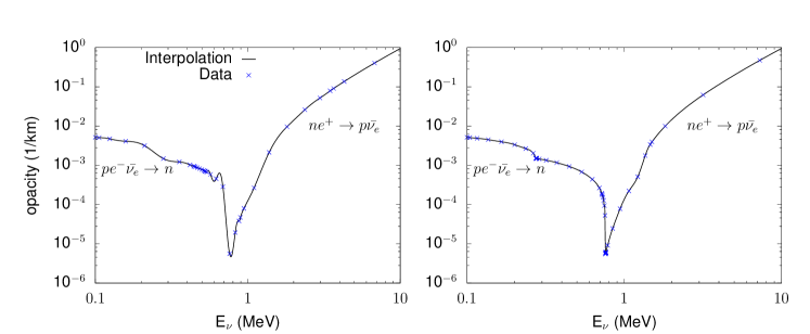
Figure 1: (color online) Example of the interpolation procedure and distribution of the energy domains in the case of a pronounced reaction threshold for $T=6$ MeV, $n_{B}=0.025$ fm^-3, $Y_{e}$ = 0.53 with RG(SLy4) EoS and RPA in Landau approximation. The crosses indicate the calculated points using five domains in energy, and the solid line corresponds to the interpolation. On the left hand side oscillations due to the Gibbs phenomenon in the interpolation function are clearly visible, whereas a better choice of the energy domains and thus a better distribution of the interpolated data points on the right hand side avoids them.

II.3.2 Interpolation procedure

For easy and fast evaluation of the neutrino opacities on the fly during simulations, we interpolate the opacity data as functions of neutrino energy and provide the coefficients for each grid point in $(T,n_{B},Y_{e})$ of the corresponding EoS data. More precisely we employ an eighth order polynomial for $\log(\kappa_{a}^{*})$ and $\log(\bar{\kappa_{a}^{*}})$ as functions of $\log(E_{\nu})$ to interpolate the opacities for (anti-)neutrino energies $E_{\nu}$ between 0.1 and 250 MeV. An additional difficulty arises if the opacities show rapid variation in a small energy interval, which can happen for instance at the different reaction thresholds which become very pronounced at low temperature. In order to avoid oscillations in the interpolation due to the Gibbs phenomenon in this case, the entire energy range $0.1\leq E_{\nu}\leq 250$ MeV is divided into several domains, where the interpolation prescription, see Eq. (35) below, is applied in each domain. The number of domains ($n_{d}$) and the domain borders $E_{\nu}^{\mathit{min/max}}$ are determined from the position of the thresholds and the variation of the opacities in the vicinity of the respective thresholds.

The energy interval $E_{\nu}\in[E_{\nu}^{\mathit{min}},E_{\nu}^{\mathit{max}}]$ has been mapped to the interval $\xi\in[-1,1]$ via an affine mapping $\log(E_{\nu})=\alpha\xi+\beta$. The opacities are then computed via

$$\log(\kappa)=\sum_{n=0}^{N}c_{n}(T,n_{B},Y_{e})\xi^{n}~{}$$ (35)

with the coefficients $c_{n}$ depending on the thermodynamic conditions and $N=8$.

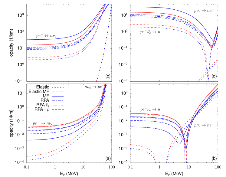
Figure 2: (color online) Neutrino (left) and anti-neutrino (right) opacities for $T=8$ MeV, $n_{B}=0.11$ fm^-3 and $Y_{e}=0.05$ (upper panels), and $T=5$ MeV, $n_{B}=0.01$ fm^-3 and $Y_{e}=0.15$ (lower panels). These correspond to typical conditions for the decoupling of neutrinos in the merger remnant Endrizzi et al. (2019), the former are more relevant for lower neutrino energies than the latter. The different line types distinguish the different approximations and results with HS(DD2) are indicated in red, whereas those with RG(SLy4) are in blue, see section II.2 for details. The dominant processes contributing to the opacities in a certain energy domain are mentioned in the figure, too.

Fig. 1 shows an example of the choice of domains to avoid an oscillating interpolation function in the case of a threshold. It corresponds to $T=6$ MeV, $n_{B}=0.025$ fm^-3, $Y_{e}$ = 0.53 and the opacities have been calculated with the RG(SLy4) EoS employing RPA in Landau approximation with a nonzero $t_{3}^{\prime}$. At low $E_{\nu}$ the reaction $p+e^{-}+\bar{\nu}\to n$ is dominant, whereas at higher energies $n+e^{+}\to p+\bar{\nu}$ overtakes. The threshold slightly below $E_{\nu}=1$ MeV is clearly visible and the opacity varies by orders of magnitude in a narrow energy interval close to this threshold. The oscillations in the interpolation on the left panel are clearly visible, whereas a better choice of domain border reduces them considerably, see the right panel.

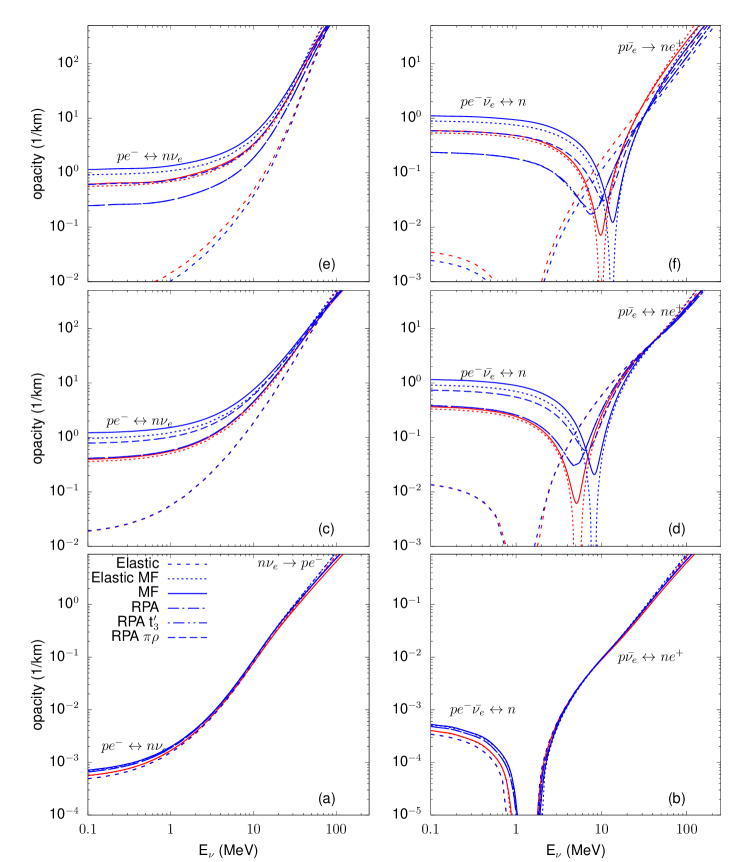
Figure 3: (color online) Neutrino (left) and anti-neutrino (right) opacities for $T=12$ MeV, $n_{B}=0.01$ fm^-3 and $Y_{e}=0.1$ (upper panels), $T=19$ MeV, $n_{B}=5\times 10^{-3}$ fm^-3 and $Y_{e}=0.1$ (middle panels) and $T=5$ MeV, $n_{B}=10^{-4}$ fm^-3 and $Y_{e}=0.1$ (lower panels). These correspond to typical conditions close to the neutrinosphere in a CCSN from our fiducial simulation, see section III. The different line types distinguish the different approximations and results with HS(DD2) are indicated in red, whereas those with RG(SLy4) are in blue. The dominant processes contributing to the opacities in a certain energy domain are mentioned in the figure, too.

II.3.3 Opacities

Let us now discuss the opacities resulting from the different approximations for various thermodynamic conditions. The most interesting regions are probably located close to the respective neutrinospheres. Since the opacities depend on neutrino energy and flavor, it is obvious that the location where neutrinos decouple from matter varies as function of these quantities. It has been observed that low energy neutrinos have in general lower opacities, i.e. longer mean free paths and decouple further inside and thus at higher densities and temperatures than high energy neutrinos.

A comprehensive analysis for binary merger simulations indicates densities $10^{-4}\lesssim n_{B}\lesssim 10^{-1}$ fm^-3 , temperatures $T\sim$ 1-10 MeV and electron fractions $Y_{e}\sim$ 0.05 - 0.3 at the corresponding neutrinospheres for neutrino energies $E_{\nu}\sim$ 3-100 MeV Endrizzi et al. (2019). The highest densities and temperatures as well as the lowest electron fractions are thereby associated with the lowest neutrino energies. Although evolving with time and being sensitive to the simulation setup, in particular the neutrino treatment and the EoS, these values can be considered as typical ones for a binary merger remnant. Fig. 2 shows the opacities employing the different approximation schemes for two different thermodynamic conditions, chosen within the above ranges. The upper panels, with $T=8$ MeV, $n_{B}=0.11$ fm^-3 and $Y_{e}=0.05$ are more relevant for neutrinos with low energies, whereas the lower panels show $T=5$ MeV, $n_{B}=0.01$ fm^-3 and $Y_{e}=0.15$, conditions close to decoupling for neutrinos with slightly higher energies.

The passage of the shock heats up matter between the proto-neutron star surface and the neutrinosphere in a CCSN such that compared with the conditions of the binary merger remnant, for CCSN we have to consider slightly higher temperatures with very similar densities and electron fractions. From our fiducial simulations, see section III, we have chosen three different thermodynamic conditions for which opacities are displayed in Fig. 3: $T=12$ MeV, $n_{B}=0.01$ fm^-3 and $Y_{e}=0.1$ (upper panels), $T=19$ MeV, $n_{B}=5\times 10^{-3}$ fm^-3 and $Y_{e}=0.1$ (middle panels) and $T=5$ MeV, $n_{B}=10^{-4}$ fm^-3 and $Y_{e}=0.1$ (lower panels). The neutrinosphere for $\bar{\nu}_{e}$ is thereby located slightly closer to the center, i.e. at slightly higher densities and temperatures. The first example (upper panels) thereby correspond roughly to conditions at the neutrinosphere for low energy $\bar{\nu}_{e}$ at early post-bounce and for $\nu_{e}$ at later times, the second is relevant for low energy anti-neutrinos and the third for both $\nu_{e}$ and $\bar{\nu}_{e}$, but with higher energies of the order ten MeV. The neutrinospheres of (anti-)neutrinos with still higher energies are located at lower densities and temperatures.

As can be seen from Fig. 3, lower panels, at $n_{B}=10^{-4}$ fm^-3, the difference between the approximation schemes is very small, the largest difference is reached for $E_{\nu}\lesssim 1$ MeV and does not exceed a factor 1.5. There are two reasons for that: first, only small momentum transfers are involved, such that the elastic approximation is well justified for the present conditions; second, as well mean field as RPA effects arise due to interactions in the dense nuclear medium and the corresponding corrections are thus small at low densities. In Table 1 we list effective masses and interaction potentials for the thermodynamic conditions of Figs. 2 and 3 and the two employed EoS and it can easily be checked that the interaction potentials are indeed small and effective masses are close to the free masses in the present case.

The situation becomes different at higher densities. At $n_{B}=5\times 10^{-3}$ fm^-3, see panel (c) and (d) in Fig. 3, momentum transfer is still small for the considered neutrino energies, such that the mean field results agree well between the elastic approximation (dotted lines) and the full phase space integration (solid lines) for both EoS. The only noticeable difference is that the opacities do not vanish any more close to the reaction thresholds upon full phase space integration, see panel (d). The mean field corrections, however, are large. The most prominent effect is the shift of the reaction threshold by $\pm\Delta U=-(m^{*}_{n}-m^{*}_{p}+U_{n}-U_{p}-(m_{n}-m_{p}))$ where the lower sign corresponds to neutrinos and the upper one to anti-neutrinos, respectively. This shift is clearly visible for the anti-neutrino opacities and it is more pronounced for RG(SLy4) since $|\Delta U|$ is larger, see Table 1. For neutrinos, no reaction threshold lies within the shown energy range. RPA correlations tend to decrease the shift in reaction threshold and push it to lower anti-neutrino energies. Both, neutrino and anti-neutrino opacities are strongly suppressed for low $E_{\nu}\lesssim 1$ MeV and approach the mean field results at higher energies. In particular, for $E_{\nu}\gtrsim 30$ MeV almost no difference is observed any more. This clearly shows, together with the shift in reaction thresholds, that RPA correlations cannot be cast into a grey correction factor, i.e. multiplying the mean field rates by a common factor for all (anti-)neutrino energies.

The prevailing role of the axial (spin-isospin) channel in the RPA results, see e.g. Reddy et al. (1999), is confirmed by the shown opacities. The vector channel is treated in the same way for all RPA models, The observed non negligible difference in the opacities is thus entirely due to the different prescriptions chosen for the axial channel, see section II.2.3. In all figures “RPA” denotes the results obtained by employing the $g_{cc}$ parameter from the standard Skyrme interaction Hernandez et al. (1999), “RPA $t_{3}^{\prime}$” those with an additional repulsive term Margueron and Sagawa (2009) and “RPA $\pi\rho$” employs the microscopically motivated $\pi\rho$-model Reddy et al. (1999). For the present case at $T=19$ MeV, $n_{B}=5\times 10^{-3}$ fm^-3 and $Y_{e}=0.1$, the $\pi\rho$ model leads to a suppression by roughly a factor 1.5 with respect to mean field results at low $E_{\nu}$, whereas for the two other RPA models the suppression is about twice as strong and reaches roughly a factor three. Similarly large differences following the prescription for the residual interaction in the axial channel are seen for other thermodynamic conditions, see Figs. 2 and 3. The uncertainties in the opacities due to this badly constrained interaction probably predominate over the differences between Landau approximation and full RPA, although the latter might become important at high densities with higher momentum transfers.

At these conditions the difference in opacities between both EoSs using the mean field approximation is almost as important as the differences between RPA and mean field results. This is no longer the case at $n_{B}=10^{-2}$ fm^-3, see Fig. 3, panels (e) and (f) as well as Fig. 2, panels (a) and (b). At low $E_{\nu}$ opacities in RPA are suppressed by about a factor five at $T=5$ MeV, $Y_{e}=0.15$ and up to a factor ten at $T=12$ MeV and $Y_{e}=0.1$, whereas the mean field results of RG(SLy4) and HS(DD2) differ only by about a factor two. The shift in the anti-neutrino reaction threshold is more pronounced for RPA, too. The opacities at higher $E_{\nu}$ again become very similar within all the different approximations employed. Please note that at neutrino energies above those shown here, momentum transfer becomes high enough to induce again noticeable differences between the results with full phase space integration and the elastic ones. At still higher densities, see Fig. 2 (upper panels), where opacities are displayed for $n_{B}=0.11$ fm^-3, $T=8$ MeV and $Y_{e}=0.05$, qualitatively the behavior is rather similar to the previously discussed cases. Quantitatively, the effect of mean field corrections increases as expected and the momentum transfer becomes higher such that the elastic mean field results no longer reproduce well the full phase space integration. The mean field calculations of Roberts and Reddy (2017) using relativistic kinematics show a similar trend: the full space integration becomes more important at higher densities when the momentum transfer becomes larger. For the particular case considered here, the three prescriptions for the residual interaction in RPA Landau approximation lead to very similar results. This should, however, not be seen as a general trend, but as a result only valid for some particular thermodynamic conditions.

The dominant processes contributing to the charged-current opacities are indicated in Figs. 2 and 3, too. Generally simulations only consider the electron and positron capture reactions as well as their inverse to compute opacities. As already noticed in Fischer et al. (2020), for low energy anti-neutrinos, (inverse) neutron decay becomes, however, the dominant charged current process under these typical thermodynamic conditions. These can even dominate over other opacity sources for low energy anti-neutrinos such as for example $NN$-Bremsstrahlung, customarily included in simulations Fischer et al. (2020). Let us emphasize that the opacities computed here and the data provided contain all different types of charged current reactions for electron (anti-)neutrinos.

From the results for the opacities discussed here, we expect for CCSN and BNS mergers that the properties of (anti-)neutrinos with an energy of tens to several tens of MeV are only slightly modified, whereas low energy (anti-)neutrinos experience more pronounced modifications. This means in particular that the resulting spectra and luminosities should be modified, too. As mentioned above, for (anti-)neutrinos with energies above those shown and discussed here, differences in opacities are expected to be due to the full phase space integration. On the one hand, within a CCSN those are not very numerous, and on the other hand their mean free path is extremely small due to the very high Fermi energy of the electrons involved in the different processes. Therefore, we will not discuss the detailed effect on their spectra here.

III Core-collapse and early proto-neutron star evolution

In this section we discuss some first results implementing the newly calculated opacities into a simulation for the early post-bounce evolution in a CCSN. These results have been obtained using a spherically-symmetric version of the CoCoNuT code Dimmelmeier et al. (2012). This code solves the general-relativistic hydrodynamics with a 3+1 decomposition of spacetime. High-resolution shock-capturing schemes are used for hydrodynamic equations, whereas Einstein equations for the gravitational field are solved with spectral methods Dimmelmeier et al. (2005). Energy losses and deleptonization via neutrino interactions are computed using the ”Fast Multi-group Transport” (FMT) scheme Müller and Janka (2015), which solves the stationary neutrino transport problem using estimates of the flux factor obtained by a two stream approximation in the optically dense region and an Eddington factor closure in the optically thin region.

Both neutrino neutral and charged currents on nuclei, along with neutral current scattering on nucleons, are considered with standard opacities in the elastic approximation Bruenn (1985) including the ion screening effect Horowitz (1997), whereas charged current neutrino nucleon opacities are the subject of this work and vary throughout the different simulations. Neither pair production reactions nor inelastic scattering have been included for electron-flavor (anti-)neutrinos. Anyway, for electron-flavor neutrinos, in the denser area of the star the medium opacity is largely dominated by charged current processes on nucleons/nuclei and the omitted reactions only play a role in equilibration of the spectrum. Heavy flavor neutrinos are treated as in Müller and Janka (2015).

The simulations start from an unstable stellar model taken among the publicly available data published by Woosley et al. (2002). All results presented in this section have been obtained using the s15 ($15M_{\odot}$ with solar metallicity) initial model, but we obtained similar conclusions by testing other progenitors, in particular with u18 ($18M_{\odot}$, $10^{-4}\times$ solar metallicity) and u40 ($40M_{\odot}$, $10^{-4}\times$ solar metallicity) progenitor models.

III.1 Pre-bounce deleptonization

Except during the last few milliseconds before trapping, pre-bounce deleptonization is dominated by electron captures on neutron-rich nuclei and the bounce properties are affected by the uncertainties on the associated rates Hix et al. (2003); Sullivan et al. (2016); Pascal et al. (2020). On the contrary, only small differences for the electron fraction at bounce are expected between different prescriptions for charged-current reactions on free nucleons.

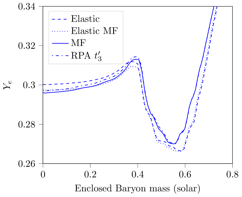
Figure 4: (color online) Profiles of the electron fraction at bounce as a function of the enclosed baryon mass, employing different approximation schemes to compute charged-current neutrino-nucleon interaction rates.

Indeed, the electron fraction profiles at bounce time are plotted in Fig. 4, for the four different models of charged-current neutrino-nucleon interaction rates. For better readability, these profiles are plotted as functions of the enclosed baryon mass (i.e. for a given radius, we consider the baryon mass contained inside this radius), which allows to take into account possible time shifts at bounce. Differences between these models remain small, showing that these reaction rates have, indeed, a small influence during the pre-bounce phase.

III.2 Post-bounce evolution

It should be stressed that our simulations have been performed in spherical symmetry, therefore the post-bounce evolution does not reflect the strong asymmetries observed in 3D simulations (see, e.g., Hanke et al. (2013)) and we cannot realistically investigate the effect of the improved rates on shock revival and post-bounce dynamics. Let us concentrate, therefore, on illustrating qualitatively the expected effects. As discussed in Section II.3.3, the main modifications should concern neutrino luminosities and spectra due to the changes in opacities for low energy (anti-) neutrinos ($E_{\nu}\lesssim 10$ MeV).

The total early post-bounce luminosities for $\nu_{e}$ and $\bar{\nu}_{e}$, with different prescriptions, as presented in Fig. 5 (for $\nu_{e}$) are very similar. The reason is that at this stage within our setup, the total luminosities are dominated by (anti-)neutrinos with energies above those for which opacities are noticeably modified. It might partly be an artifact of the approximations within the FMT neutrino treatment, where in particular inelastic scattering reactions are neglected, which contribute to redistributing neutrino energies and could thus lead to having more low energy neutrinos in the spectrum. We also expect stronger modifications of luminosities at later times, when emitted neutrinos have a mean energy of the order of a few $\mathrm{MeV}$.

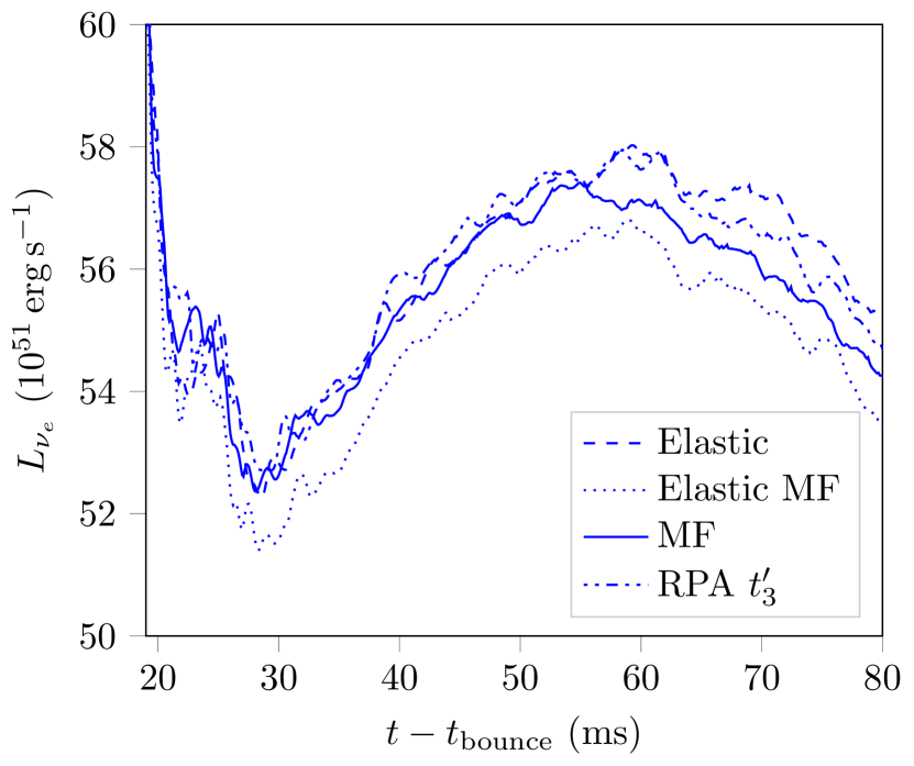
Figure 5: (color online) Total neutrino luminosities as a function of time after bounce.

The modified opacities for low energy (anti-)neutrinos clearly affect the location of the neutrinospheres. Here, we have defined them as the radius where optical depth reaches $2/3$. In Fig. 6, upper panel, the neutrinospheres for $\nu_{e}$ (left) and $\bar{\nu_{e}}$ (right) with an energy of $E_{\nu}=2$ MeV are displayed, employing the different prescriptions for the charged-current opacities. The results for the opacities for typical conditions discussed in Section II.3.3 are clearly reflected in the position of the neutrinosphere. Increased opacities due to mean field effects compared with the basic elastic approximation make it more difficult for (anti-)neutrinos to escape and lead therefore to a neutrinosphere at larger radii. On the other hand, a reduction of opacities within RPA with respect to mean field facilitates escape and shifts the neutrinosphere again to smaller radii. As anticipated, for larger neutrino energies, the difference becomes smaller, see the example for $E_{\nu}=14$ MeV in the lower panel of Fig. 6.

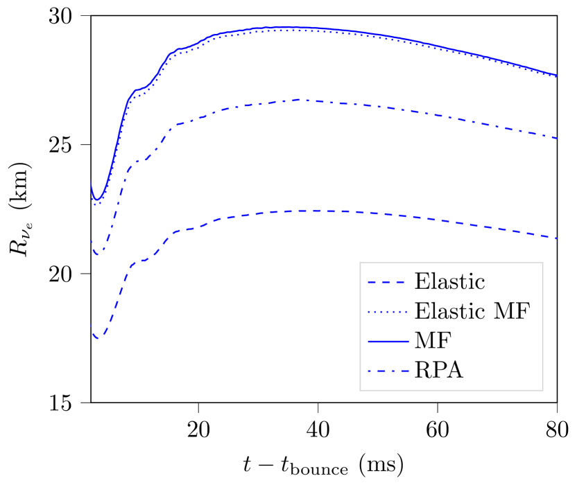
(a) Electron neutrino $\nu_{e}$, energy $E_{\nu}=$2\text{\,}\mathrm{MeV}$$

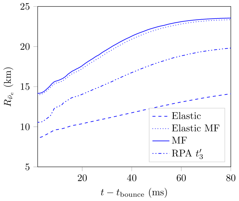
(b) Electron antineutrino $\bar{\nu}_{e}$, energy $E_{\nu}=$2\text{\,}\mathrm{MeV}$$

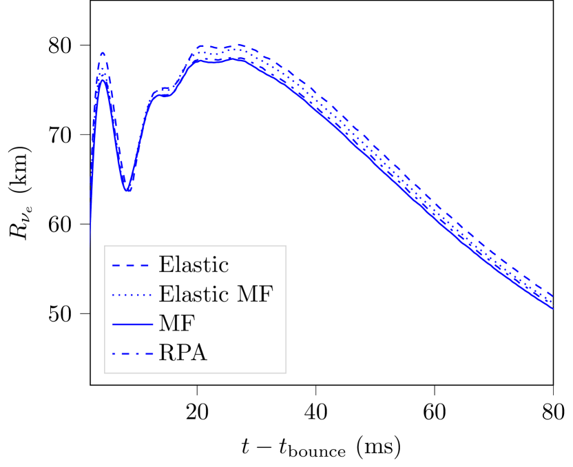
(c) Electron neutrino $\nu_{e}$, energy $E_{\nu}=$14\text{\,}\mathrm{MeV}$$

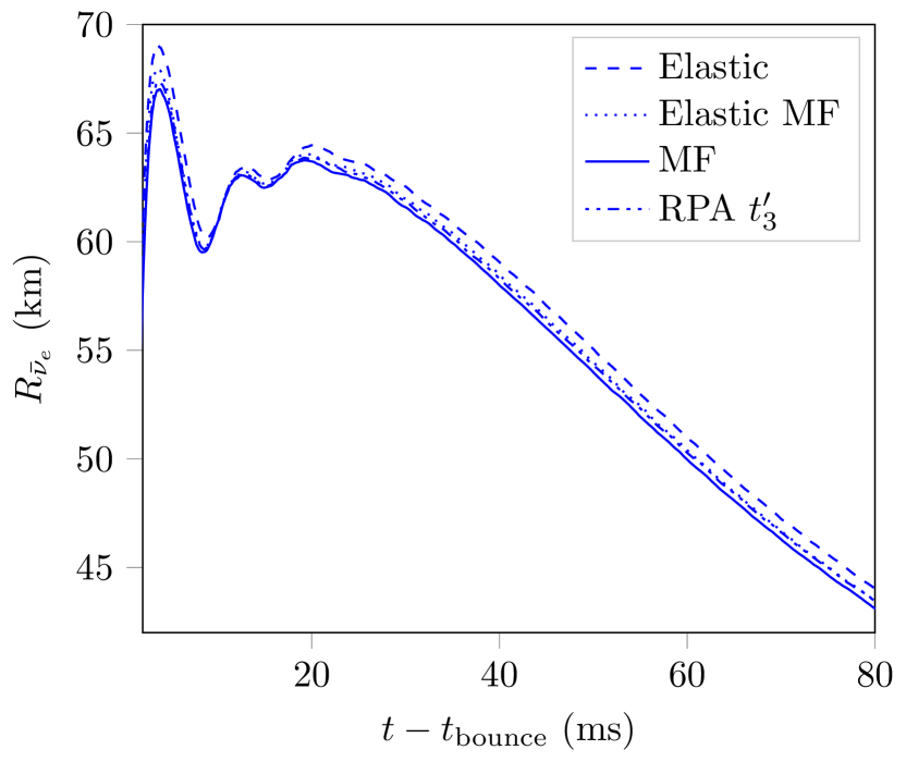
(d) Electron antineutrino $\bar{\nu}_{e}$, and energy $E_{\nu}=$14\text{\,}\mathrm{MeV}$$

Figure 6: Neutrinospheres radius as a function of time after bounce, for two different neutrinos energies.

IV Summary and discussion

Within this work we have computed opacities for $\nu_{e}$ and $\bar{\nu}_{e}$ from charged current neutrino-nucleon interactions, going beyond the elastic approximation and including nuclear correlations in RPA. Please note that we do not pretend here that our opacity data represent the ultimate description of nuclear correlations. The differences in opacities induced by the different prescriptions for evaluating the axial channel give an idea about the uncertainties within RPA. Moreover, it only takes into account a certain class of correlations, the long-range linear response. It is, however, known since many years that these more accurate calculations beyond the elastic approximation induce important changes in the opacities in dense matter Reddy et al. (1998, 1999); Burrows and Sawyer (1999) and are therefore susceptible to modify the dynamics of CCSN and matter composition in BNS mergers. Hence, we have presented here a first step, proposing a scheme which allows to incorporate accurate opacities directly into numerical simulations which otherwise would be too time consuming to be calculated “on the fly”. We have been able to perform CCSN simulations with consistently computed accurate charged current (electron) neutrino nucleon interactions. We find noticeable differences in the location of the neutrinospheres of low-energy (anti-)neutrinos in the early post-bounce phase. In Fischer et al. (2020), where rates in mean field with full phase space are compared with the elastic approximation, during the longer term proto-neutron star evolution in particular changes in the mean energies of $\bar{\nu_{e}}$ and in the composition of the neutrino-driven wind, i.e. the conditions for nucleosynthesis, are pointed out. We expect the RPA correlations to impact these quantities as well, a detailed study will be carried out in future work. It should be stressed at this point that the modifications in the opacities with respect to the commonly employed elastic approximation strongly depend on neutrino energy and therefore cannot be cast into a grey correction factor to the analytic expressions as previously implemented in simulations.

After SN 1987A, much progress has been made and a possible neutrino signal observed from a galactic supernova in present day detectors would bear essential information about the core collapse mechanism and neutrino properties Mirizzi et al. (2016). It is therefore crucial that models use accurate neutrino matter interaction rates. As prospected since more than twenty years Reddy et al. (1998, 1999); Burrows and Sawyer (1998, 1999), this work represents a first step in enabling the use of these accurate rates in CCSN simulations. It focuses on charged current neutrino nucleon opacities and clearly shows that, indeed, commonly employed approximations break down in the dense central part. These results encourage on the one hand to go beyond our simplified setup for the simulations (spherical symmetry, simplified neutrino transport) and to include these accurate rates in more sophisticated simulations, in order to study in details not only bounce properties but shock and post-bounce dynamics, too, and the corresponding neutrino signal. To that end, the tables with our opacity data are publicly available within the Compose data base. A non-optimized implementation of the tables within our code leads to maximally 50% increase in computing time with respect to standard analytic formulae. This is probably an upper limit since the FMT does not include inelastic $\nu_{e}$-$e^{\pm}$ scattering which is in general much more time consuming than charged-current opacities. On the other hand, efforts should be pursued to extend the present scheme for neutrino rates to other channels and offer ultimately the possibility to include neutrino-matter interactions with state-of-the art input physics within simulations. In particular, we have only considered improved opacities for charged current neutrino-nucleon interactions. Their increase in the dense regions makes them largely dominant, whereas with the standard approximations neutral current opacities are of the same order of magnitude. The sensitivity of CCSN dynamics to the detailed treatment of the neutral currents has been shown in Melson et al. (2015), too, where a small change in the coupling constants due to the strangeness content of the nucleon decides upon explosion. A consistent implementation of improved neutral current opacities Reddy et al. (1998, 1999); Burrows and Sawyer (1998); Navarro et al. (1999); Margueron et al. (2004); Horowitz and Schwenk (2006); Horowitz et al. (2017) is thus in order and shall be investigated in future work. Among others, we expect it to influence the relation between neutrino trapping and the onset of $\beta$-equilibrium.

Appendix A Format of the opacity tables

Data for (anti-)neutrino opacities are provided using the HDF5data format The HDF Group (2020). Two HDF5groups, nu and nu_bar, contain the necessary data to evaluate the respective opacities for $\nu_{e}$ and $\bar{\nu}_{e}$ via the interpolation scheme discussed in Sec. II.3.2. In each group are stored the following attributes: the information on the maximum number $n_{d}^{\mathit{max}}$ ( attribute nd_max) of domains in $E_{\nu}$, the number of grid points for temperature $i_{T}$ (pts_t), for baryon number density $j_{B}$ (pts_nb) and for electron fraction $k_{Y}$ (pts_ye) as well as the number $n_{p}$ (npts) of interpolation coefficients. Within each group, four datasets exist: nd_tny, enumin, enumax, and coeffs. nd_tny contains an array of size ($i_{T},j_{B},k_{Y}$) with the number $n_{d}$ of domains in $E_{\nu}$ for each point on the grid in $(T,n_{B},Y_{e})$ of the EoS table. The two datasets enumin and enumax contain arrays of size ($n_{d}^{\mathit{max}},i_{T},j_{B},k_{Y}$). The first $n_{d}$ nonzero entries contain, respectively, the logarithm of the minimum and maximum energy in each domain for each point on the EoS grid. The dataset coeffs is the array containing the coefficients $c_{n}$ in Eq. (35) in all domains and for the entire EoS grid. The structure of the HDF5 file is summarized in Table 2.

Name	Quantity	Type
		(size)
npts	$n_{p}=N+1$: number of	integer
	interpolation coefficients $c_{n}$
	with $n\in(0,\dots,N)$
pts_t	number $i_{T}$ of points in $T$	integer
pts_nb	number $j_{B}$ of points in $n_{B}$	integer
pts_ye	number $k_{Y}$ of points in $Y_{e}$	integer
nd_tny	number $n_{d}$ of domains	array of integers
	in $E_{\nu}$ for each	($i_{T},j_{B},k_{Y}$)
	grid point in $(T,n_{B},Y_{e})$
nd_max	$n_{d}^{\mathit{max}}=\mathrm{max}(n_{d})$ : maximum	array of integers
	number of domains in $E_{\nu}$
enumin	logarithm of minimum $E_{\nu}$	array of doubles
	in each domain for each	($n_{d}^{\mathrm{max}},i_{T},j_{B},k_{Y}$)
	grid point in $(T,n_{B},Y_{e})$
enumax	logarithm of maximum $E_{\nu}$	array of doubles
	in each domain for each	($n_{d}^{\mathrm{max}},i_{T},j_{B},k_{Y}$)
	grid point in $(T,n_{B},Y_{e})$
coeffs	interpolation coefficients $c_{n}$	array of doubles
	in each domain and for each	($n_{p},n_{d}^{\mathrm{max}},i_{T},j_{B},k_{Y}$)
	grid point in $(T,n_{B},Y_{e})$

Table 2: Summary of the structure of the HDF5 file storing the opacity data for $\nu_{e}$ (group nu) and $\bar{\nu}_{e}$ (group nu_bar).

We have considered that the detail values of the opacity were irrelevant when the mean free path became (much) larger than the extension of the studied astrophysical object, and therefore a lower bound for $\kappa$ has been introduced: for all $\kappa<\kappa_{\mathit{limit}}=10^{-10}$/km, we have set $\kappa=\kappa_{\mathit{limit}}$ in the data tables.

Appendix B Lindhard function in asymmetric matter

Eq. (28) for the Lindhard function can be further developed by substituting in the last term $\vec{k}\to-\vec{k}-\vec{q}$

$$L(q) =\lim_{\eta\to 0}\int\frac{d^{3}k}{(2\pi)^{3}}\left(\frac{f_{F}(\epsilon_{k}^{p}-\mu_{p}^{*})}{\tilde{q_{0}}+i\eta+\epsilon_{k}^{p}-\epsilon_{k+q}^{n}}\right.$$

$$\qquad\qquad\qquad{}-\left.\frac{f_{F}(\epsilon_{k}^{n}-\mu_{n}^{*})}{\tilde{q_{0}}+i\eta+\epsilon_{k+q}^{p}-\epsilon_{k}^{n}}\right)~{}.$$ (36)

The angular integration can be performed analytically using $\epsilon_{k+q}^{i}=(\vec{k}+\vec{q})^{2}/(2m_{i}^{*})+m_{i}^{*}$. Thus,

$$L(q) =\frac{1}{4\pi^{2}|\vec{q}|}\;\lim_{\eta\to 0}\int kdk\times$$

$$\qquad\qquad{}\left(\int_{\epsilon_{-}^{n}}^{\epsilon_{+}^{n}}dx\;m_{n}\frac{f_{F}(\epsilon_{k}^{p}-\mu^{*}_{p})}{\tilde{q_{0}}+i\eta+\epsilon_{k}^{p}-x}\right.$$

$$\qquad\qquad{}-\int_{\epsilon_{-}^{p}}^{\epsilon_{+}^{p}}dx\left.m_{p}\frac{f_{F}(\epsilon_{k}^{n}-\mu^{*}_{n})}{\tilde{q_{0}}+i\eta+x-\epsilon_{k}^{n}}\right)$$

$$=-\frac{1}{4\pi^{2}|\vec{q}|}\;\lim_{\eta\to 0}\int kdk\times$$

$$\left(m_{n}f_{F}(\epsilon_{k}^{p}-\mu_{p}^{*})\log\left(\frac{\epsilon_{+}^{n}-\tilde{q_{0}}-i\eta-\epsilon_{k}^{p}}{\epsilon_{-}^{n}-\tilde{q_{0}}-i\eta-\epsilon_{k}^{p}}\right)\right.$$

$$+\left.m_{p}f_{F}(\epsilon_{k}^{n}-\mu_{n}^{*})\log\left(\frac{\epsilon_{+}^{p}+\tilde{q_{0}}+i\eta-\epsilon_{k}^{n}}{\epsilon_{-}^{p}+\tilde{q_{0}}+i\eta-\epsilon_{k}^{n}}\right)\right)~{}.$$ (37)

The integration boundaries are given by

$$\epsilon_{\pm}^{i}=\frac{(|\vec{k}|\pm|\vec{q}|)^{2}}{2m_{i}^{*}}+m^{*}_{i}~{}.$$ (38)

For the real part, the remaining integration over momentum in Eq. (37) has to be carried out numerically. Alternatively, the real part can be obtained from a dispersion integral with the analytic expression of the imaginary part, see Eq. (43) below.

Using the technique indicated in Reddy et al. (1998) we can give an analytic expression for the imaginary part of the Lindhard function in the case of non-interacting particles or in mean field. To that end we rewrite it as, see Eq. (37)

$$\mathrm{Im}\,L(q) =-\frac{1}{4\pi|\vec{q}|}\int kdk\times$$

$$\left(\int_{\epsilon_{-}^{n}}^{\epsilon_{+}^{n}}dx\;m_{n}f_{F}(\epsilon_{k}^{p}-\mu^{*}_{p})\,\delta(\tilde{q_{0}}+\epsilon_{k}^{p}-x)\right.$$

$$-\int_{\epsilon_{-}^{p}}^{\epsilon_{+}^{p}}dx\left.m_{p}f_{F}(\epsilon_{k}^{n}-\mu^{*}_{n})\,\delta(\tilde{q_{0}}+x-\epsilon_{k}^{n})\right)$$ (39)

The angular integration can be evaluated with the help of the $\delta$-function and we obtain

$$\mathrm{Im}L(q) =-\frac{1}{4\pi\,|\vec{q}|}\left(m^{*}_{n}\int_{k_{-}^{p}}^{k_{+}^{p}}kdk\,\,f_{F}(\epsilon_{k}^{p}-\mu^{*}_{p})\right.$$

$$\qquad{}\left.-m^{*}_{p}\int_{k_{-}^{n}}^{k_{+}^{n}}kdk\,f_{F}(\epsilon_{k}^{n}-\mu^{*}_{n})\right)~{},$$ (40)

where $k_{\pm}^{i}$ is given by the boundaries on the angular integration,

$$k_{\pm}^{i} =\left|\frac{\pm m_{i}^{*}|\vec{q}|+X}{m_{n}^{*}-m_{p}^{*}}\right|$$ (41)

$$X =\left(m_{n}^{*}m_{p}^{*}\,(\vec{q}^{2}+2\,(m_{n}^{*}-m_{p}^{*})\,(m_{n}^{*}-m_{p}^{*}-\tilde{q_{0}}))\right)^{1/2}$$

The remaining integration can be carried by employing Eq. (20) of Ref. Reddy et al. (1998) with $x_{i}T=\vec{k}^{2}/(2m_{i}^{*})+m_{i}^{*}-\mu_{i}^{*}$

$$\mathrm{Im}L(q)=-\frac{Tm_{n}^{*}m_{p}^{*}}{4\pi\,|\vec{q}|}\left(\int_{x_{-}^{p}}^{x_{+}^{p}}\frac{dx}{e^{x}+1}-\int_{x_{-}^{n}}^{x_{+}^{n}}\frac{dx}{e^{x}+1}\right)~{},$$ (42)

where $x_{\pm}^{i}=((k^{i}_{\pm})^{2}/(2m_{i}^{*})+m_{i}^{*}-\mu_{i}^{*})/T$. The final integration leads to

$$\mathrm{Im}L(q)=\frac{Tm_{n}^{*}m_{p}^{*}}{4\pi\,|\vec{q}|}\left\{\ln\left(\frac{1+e^{-x_{+}^{n}}}{1+e^{-x_{-}^{n}}}\right)-\ln\left(\frac{1+e^{-x_{+}^{p}}}{1+e^{-x_{-}^{p}}}\right)\right\}~{}.$$ (43)

The result, apart from being written in a more symmetric way, agrees with that from Reddy et al. (1998), Eq. (41), if the different definition of $q_{0}$ is considered, which cancels here the explicit $\mu_{p}-\mu_{n}$-term in the argument of the logarithm. In addition, the factor $(1+f_{B}(q_{0}))$ is absent since it is explicitly accounted for in Eq. (11).

Appendix C Opacity expressions

As mentioned in section II.1, the contribution of positronic processes to the opacities can be obtained straightforwardly by replacing $(E_{e},\vec{k_{e}})\to-(E_{e},\vec{k_{e}})$ in the expressions for electronic processes. The complete emissivity and mean free path for neutrinos including reactions $p+e^{-}\leftrightarrow n+\nu_{e}$ and $p\leftrightarrow n+e^{+}+\nu_{e}$ becomes then

$$j(E_{\nu})= -\frac{G_{F}^{2}V_{ud}^{2}}{8}\int\frac{d^{3}k_{e}}{(2\pi)^{3}}\frac{1}{E_{e}E_{\nu}}\times$$

$$\left\{L^{\lambda\sigma}\mathrm{Im}\Pi^{R}_{\lambda\sigma}(q)\times\right.$$

$$\qquad f_{F}(E_{e}-\mu_{e}))\,(1+f_{B}(q_{0}))$$

$$+ L^{\lambda\sigma}\mathrm{Im}\Pi^{R}_{\lambda\sigma}(q^{+})\times$$

$$\left.\qquad(1-f_{F}(E_{e}+\mu_{e}))\,(1+f_{B}(q_{0}^{+}))\right\}$$

$$\frac{1}{\lambda(E_{\nu})}= -\frac{G_{F}^{2}V_{ud}^{2}}{8}\int\frac{d^{3}k_{e}}{(2\pi)^{3}}\frac{1}{E_{e}E_{\nu}}\times$$

$$\left\{L^{\lambda\sigma}\mathrm{Im}\Pi^{R}_{\lambda\sigma}(q)\times\right.$$

$$\qquad(1-f_{F}(E_{e}-\mu_{e}))\,f_{B}(q_{0})$$

$$+ L^{\lambda\sigma}\mathrm{Im}\Pi^{R}_{\lambda\sigma}(q^{+})\times$$

$$\left.\qquad f_{F}(E_{e}+\mu_{e})\,f_{B}(q_{0}^{+})\right\}$$ (44)

with $q^{+}=(-E_{e}-E_{\nu}-\mu_{e}+\mu_{\nu},-\vec{k_{e}}-\vec{k_{\nu}})$. For anti-neutrinos it becomes, including $n\leftrightarrow p+e^{-}+\bar{\nu}_{e}$ and $n+e^{+}\leftrightarrow p+\bar{\nu}_{e}$ reactions

$$\bar{\jmath}(E_{\nu})= -\frac{G_{F}^{2}V_{ud}^{2}}{8}\int\frac{d^{3}k_{e}}{(2\pi)^{3}}\frac{1}{E_{e}E_{\nu}}\times$$

$$\left\{L^{\lambda\sigma}\mathrm{Im}\Pi^{R}_{\lambda\sigma}(\bar{q})\times\right.$$

$$\qquad(1-f_{F}(E_{e}-\mu_{e}))\,f_{B}(\bar{q_{0}})$$

$$+ L^{\lambda\sigma}\mathrm{Im}\Pi^{R}_{\lambda\sigma}(\bar{q}^{+})\times$$

$$\qquad\left.f_{F}(E_{e}+\mu_{e})\,f_{B}(\bar{q_{0}}^{+})\right\}$$

$$\frac{1}{\bar{\lambda}(E_{\nu})}= -\frac{G_{F}^{2}V_{ud}^{2}}{8}\int\frac{d^{3}k_{e}}{(2\pi)^{3}}\frac{1}{E_{e}E_{\nu}}\times$$

$$\left\{L^{\lambda\sigma}\mathrm{Im}\Pi^{R}_{\lambda\sigma}(\bar{q})\times\right.$$

$$\qquad f_{F}(E_{e}-\mu_{e})\,(1+f_{B}(\bar{q_{0}}))$$

$$+ L^{\lambda\sigma}\mathrm{Im}\Pi^{R}_{\lambda\sigma}(\bar{q}^{+})\times$$

$$\qquad(1-f_{F}(E_{e}+\mu_{e}))\,(1+f_{B}(\bar{q_{0}}^{+}))$$ (45)

with $\bar{q}^{+}=(-E_{e}+E_{\nu}-\mu_{e}+\mu_{\nu},-\vec{k_{e}}+\vec{k_{\nu}})$. The simple properties, cf Eq. (15),

$$(1-f_{F}(E_{e}+\mu_{e}))\,(1+f_{B}(q_{0}^{+}))=$$

$$\quad f_{B}(q_{0}^{+})f_{F}(E_{e}+\mu_{e})\exp((-E_{\nu}+\mu_{\nu})/T)~{},$$

$$(1-f_{F}(E_{e}+\mu_{e}))\,(1+f_{B}(\bar{q_{0}}^{+}))=$$

$$\quad f_{B}(\bar{q_{0}}^{+})f_{F}(E_{e}+\mu_{e})\exp((E_{\nu}+\mu_{\nu})/T)~{},$$ (46)

reflect detailed balance for positronic processes as it should. In terms of emissivity and mean free path detailed balance reads

$$j(E_{\nu}) =\frac{\exp((-E_{\nu}+\mu_{\nu})/T)}{\lambda(E_{\nu})}$$

$$\bar{\jmath}(E_{\nu}) =\frac{\exp((-E_{\nu}-\mu_{\nu})/T)}{\bar{\lambda}(E_{\nu})}~{}.$$ (47)

For practical purposes, the integration over electron momenta can be transformed into an integration over $q_{0}$ and $|\vec{q}|$. For instance, considering the reactions with electrons and neutrinos, $p+e^{-}\leftrightarrow n+\nu_{e}$, we can use

$$\vec{q}^{2}=\vec{k_{e}}^{2}+E_{\nu}^{2}-2|\vec{k_{e}}|E_{\nu}z~{},$$ (48)

and $q_{0}=E_{e}-E_{\nu}-\mu_{e}+\mu_{\nu}$ to obtain

$$\int\frac{d^{3}k_{e}}{(2\pi)^{3}} =\frac{1}{4\pi^{2}}\int|\vec{k_{e}}|E_{e}dE_{e}\int_{-1}^{1}dz$$

$$=\frac{1}{4\pi^{2}}\int_{m_{e}-E_{\nu}-\mu_{e}+\mu_{\nu}}^{\infty}\frac{E_{e}}{E_{\nu}}dq_{0}\int_{|k-E_{\nu}|}^{k+E_{\nu}}|\vec{q}|d|\vec{q}|~{},$$ (49)

with $k=|\vec{k_{e}}|$.

In elastic approximation, cf Eq. (20), neutrino emissivity becomes

$$j(E_{\nu}) =\frac{G_{F}^{2}V_{ud}^{2}}{\pi}\,(g_{V}^{2}+3g_{A}^{2})(n_{p}-n_{n})\,(1+f_{B}(q_{0}))\times$$

$$\left(k_{e^{-}}E_{e^{-}}\,f_{F}(E_{e^{-}}-\mu_{e})\right.$$

$$+\left.k_{e^{+}}E_{e^{+}}\,(1-f_{F}(E_{e^{+}}+\mu_{e}))\right)~{},$$ (50)

with $E_{e^{\pm}}=\mp(E_{\nu}+m_{n}-m_{p})$ and $q_{0}=m_{n}-m_{p}+\mu_{p}-\mu_{n}$. $k_{e^{\pm}}=\sqrt{E_{e^{\pm}}^{2}-m_{e}^{2}}$ denotes the momentum of the charged lepton. For anti-neutrinos we have

$$\bar{\jmath}(E_{\nu}) =\frac{G_{F}^{2}V_{ud}^{2}}{\pi}\,(g_{V}^{2}+3g_{A}^{2})(n_{p}-n_{n})\,f_{B}(q_{0})\times$$

$$\left(k_{e^{-}}E_{e^{-}}\,(1-f_{F}(E_{e^{-}}-\mu_{e}))\right.$$

$$+\left.k_{e^{+}}E_{e^{+}}\,f_{F}(E_{e^{+}}+\mu_{e})\right)~{},$$ (51)

with $E_{e^{\pm}}=\mp(-E_{\nu}+m_{n}-m_{p})$ and $q_{0}=m_{n}-m_{p}+\mu_{p}-\mu_{n}$. The mean free paths are then given by Eqs. (47). Corrected for mean field effects this becomes for neutrinos

$$j(E_{\nu}) =\frac{G_{F}^{2}V_{ud}^{2}}{\pi}\,(g_{V}^{2}+3g_{A}^{2})\eta_{pn}\times$$

$$\left(k_{e^{-}}E_{e^{-}}\,f_{F}(E_{e^{-}}-\mu_{e})\right.$$

$$+\left.k_{e^{+}}E_{e^{+}}\,(1-f_{F}(E_{e^{+}}+\mu_{e}))\right)~{},$$ (52)

with $E_{e^{\pm}}=\mp(E_{\nu}+m_{n}^{*}-m_{p}^{*}+U_{n}-U_{p})$ and $k_{e^{\pm}}=\sqrt{E_{e^{\pm}}^{2}-m_{e}^{2}}$. For anti-neutrinos

$$\bar{\jmath}(E_{\nu}) =\frac{G_{F}^{2}V_{ud}^{2}}{\pi}\,(g_{V}^{2}+3g_{A}^{2})\eta_{np}\times$$

$$\left(k_{e^{-}}E_{e^{-}}\,(1-f_{F}(E_{e^{-}}-\mu_{e}))\right.$$

$$+ \left.k_{e^{+}}E_{e^{+}}\,f_{F}(E_{e^{+}}+\mu_{e})\right)~{},$$ (53)

with $E_{e^{\pm}}=\mp(-E_{\nu}+m_{n}^{*}-m_{p}^{*}+U_{n}-U_{p})$.