Parametrisations of relativistic energy density functionals with tensor couplings

Abstract

The relativistic density functional with minimal density dependent nucleon-meson couplings for nuclei and nuclear matter is extended to include tensor couplings of the nucleons to the vector mesons. The dependence of the minimal couplings on either vector or scalar densities is explored. New parametrisations are obtained by a fit to nuclear observables with uncertainties that are determined self-consistently. The corresponding nuclear matter parameters at saturation are determined including their uncertainties. An improvement in the description of nuclear observables, in particular for binding energies and diffraction radii, is found when tensor couplings are considered, accompanied by an increase of the Dirac effective mass. The equations of state for symmetric nuclear matter and pure neutron matter are studied for all models. The density dependence of the nuclear symmetry energy, the Dirac effective masses and scalar densities is explored. Problems at high densities for parametrisations using a scalar density dependence of the couplings are identified due to the rearrangement contributions in the scalar self-energies that lead to vanishing Dirac effective masses.

1 Introduction

Since the application of the relativistic mean-field (RMF) approach in the framework of quantum hadron dynamics, various kinds of a relativistic energy density functionals (EDFs) have been developed in the theoretical description of atomic nuclei and nuclear matter, see, e.g., Serot:1984ey ; Reinhard:1989zi ; Ring:1996qi ; Meng:2016 . In these types of phenomenological approaches the strong interaction between nucleons is described in an effective way by the exchange of mesons. In most cases a minimal coupling of mesons to the nucleons is considered with a strength that is determined by the corresponding coupling constants. As a result every nucleon $i$ moves in vector ($V_{i}$) and scalar ($S_{i}$) mean fields. Although the effective interaction in an EDF shares some similarities with realistic one-boson exchange (OBE) potentials due to general features of the strong interaction, it has a more simplistic structural form and cannot describe the free nucleon-nucleon scattering quantitatively. The model parameters are treated as independent quantities without assuming constraints from theoretical considerations, e.g., relations between different couplings as in OBE potentials. The coupling strengths between mesons and nucleons in the EDF are usually obtained by fitting the model predictions of nuclear observables to experimental data. Sometimes also nuclear matter parameters, which are extracted indirectly from properties of nuclei or experiments with heavy-ion collisions, are used as constraints. In order to obtain a good quantitative description, a medium dependence of the effective interaction has to be considered. This is most often realized by nonlinear self-couplings of the mesons or a density dependence of the nucleon-meson couplings. Many parametrisations Dutra:2014qga have been developed for different applications. The effects of other types of interaction vertices, e.g., with derivative couplings Typel:2002ck ; Typel:2005ba ; Gaitanos:2009nt ; Gaitanos:2011yb ; Gaitanos:2011ej ; Chen:2012rn ; Gaitanos:2012hg ; Chen:2014 ; Gaitanos:2015xpa ; Antic:2015tga or tensor couplings, are less intensively explored.

Relativistic EDFs are derived originally in the mean-field or Hartree approximation starting from a covariant Lagrangian density with nucleon and meson fields as degrees of freedom. This means that the many-nucleon wave function is a simple product of single particle states that are occupied according to Fermi-Dirac statistics but an explicit antisymmetrisation of the many-nucleon wave function, e.g., in form of a Slater determinant, is not considered. Only later, exchange or Fock terms were taken into account in the construction of relativistic EDFs, usually called relativistic Hartree-Fock (RHF) models, see, e.g., Horowitz:1982kp ; Bouyssy:1987sh ; Bernardos:1993re ; Long:2005ne ; Long:2008fm . In this work the relativistic Hartree approach is utilized because it is more transparent and less involved from a computational point of view. Density dependent meson-nucleon couplings in a full RHF model with finite-range interactions would also introduce some complications in the derivation of the field equations that are difficult to treat completely self-consistently in actual calculations.

The first parametrisation of a RMF model with $\omega$ and $\rho$ tensor couplings, VT, found from a fit to nuclear observables, was introduced in Rufa:1988zz . A systematic variation of the coupling strengths showed no strong sensitivity of most observables to the tensor contributions and only a slight improvement with a finite $\omega$ tensor coupling. However, a decrease of the incompressibility $K$ of nuclear matter and larger effective nucleon masses were found. The application of RMF calculations with a $\rho$ tensor coupling was extended from spherical to deformed nuclei in Jian-Kang:1991hco . The dependence of spin-orbit splittings on the strength of the $\rho$ tensor coupling was explored in Ren:1995 . Adding a $\rho$ tensor coupling to existing RMF parametrisations, the modification of the neutron skin thickness of nuclei was studied later in Jiang:2005vu . Tensor coupling terms were derived from a systematic expansion in an effective approach using chiral symmetry in Furnstahl:1996wv and two new parametrisations, G1 and G2, were obtained by a fit to nuclear observables with much stronger $\rho$ tensor couplings than $\omega$ tensor couplings. The effects on spin-orbit splittings and the effective mass were studied in Furnstahl:1997tk . Small effects were found in another parametrisation, NL-VT1, determined in the framework of RMF models with nonlinear self-couplings of the mesons, which was applied to the study of super-heavy nuclei Bender:1999yt . The same interaction was used in Sulaksono:2005ac for a comparison of single-particle spectra in comparison to other EDFs. The modification of nuclear magnetic moments by isoscalar tensor couplings was already investigated in Bouyssy:1984bg and a possible origin in the framework of RMF models was discussed there. Tensor couplings of nucleons to $\omega$ and $\rho$ mesons in RHF calculations were considered first in Bouyssy:1987sh and several studies followed. For instance, in Long:2006pn the influence of tensor couplings on pseudospin-orbit splittings was investigated, and in Long:2007dw a new parametrisation, PKA1, for RHF calculations with density dependent couplings was introduced. The effects on the evolution of shell gaps and spin-orbits splittings were explored in Wang:2012nu and in Jiang:2014mca , respectively, in comparison to other relativistic EDFs. Another series of RHF parametrisations was presented in Liliani:2016npj with an extensive exploration of the effects. The Zimanyi-Moszkowski version of the RMF Lagrangian was generalized in Biro:1996nk with a $\omega$ tensor coupling contribution to increase the small spin-orbit splitting of the original model. In spite of all these investigations no comprehensive understanding of the role and importance of tensor couplings in relativistic EDFs has been reached and, hence, they are usually not taken into account in most models.

A specific feature of tensor couplings is the fact that they contribute to the strength of the spin-orbit splitting in nuclei. In standard RMF calculations of spherical nuclei the size of the energy splitting between single-nucleon levels of identical orbital angular momentum $l$ but different total angular momentum $j=l\pm 1/2$ is tightly correlated with the scalar potential $S_{i}$ and the Dirac effective mass $m_{i}^{\ast}=m_{i}-S_{i}$ of a nucleon $i$ with vacuum mass $m_{i}$. The introduction of tensor couplings can lift this correlation and allows to increase the effective mass that is usually considered to be smaller than expected to describe the level density near the Fermi energy. In calculations of nuclear matter, however, tensor couplings do not contribute in the conventional mean-field approximation of spatially uniform systems since their effect depends on spatial derivatives of densities.

It was realized early on that an effective medium dependence of the interaction has to be included in relativistic approaches in order to improve the description of nuclei and nuclear matter quantitatively. One major class of models considers a self-coupling or cross-coupling of the mesons leading to an increase of the number of model parameters. A second class introduces a density dependence of the meson-nucleon couplings. It can be arbitrarily varied depending on the selected form of the function. In addition, a specific feature of relativistic models can be exploited in this approach. There are various types of densities and currents that can be formed in a Lorentz covariant way from the nuclear wave functions and that can enter as argument in the coupling functions. The most common approach is a so-called vector density dependence. In contrast, scalar or other density dependencies are hardly used in recent EDF parametrisations even though they were discussed in some of the first applications of the RMF model Fuchs:1995as ; Lenske:1995wyj . Depending on the choice of a vector or scalar density dependence, so-called rearrangement terms appear in the vector or scalar mean fields, respectively, in addition to the regular meson contributions. They are essential for the thermodynamic consistency of the theory. Differences between models with different density dependencies seem to be small in the density range where they are constrained by nuclear data but problems may arise is some parts of the phase diagram of nuclear matter under particular conditions Typel:2018cap .

In this work a new set of parametrisations for relativistic EDFs is introduced with a vector or a scalar density dependence of the couplings and the effects of tensor couplings are studied. The model parameters are usually determined by minimising an objective function that depends on the differences between calculated and measured nuclear data weighted by (inverse) uncertainties. The latter are mostly set heuristically to certain fixed values. These are assumed to be of reasonable size matching the expected quality of the model. These uncertainties are generally larger than the experimental errors of the considered nuclear data. Here a modified approach is followed. It allows to adjust the uncertainties during the determination of the model parameters in the fitting procedure, see, e.g., Dobaczewski:2014jga . Thus the uncertainties are obtained in a self-consistent way and give a new possibility to judge the quality of the EDF.

The approach presented here stays on the mean-field level and does not consider any effects beyond this approximation. Beyond mean-field effects are known to have a noticeable impact, e.g., on single-particle spectra and excited states of nuclei which are, however, not examined in this work. There are different ways of treating beyond mean-field effects, e.g., by studying collective correlations and their fluctuations related to the restoration of broken symmetries or by applying (quasi-particle) random phase approximation (RPA) methods looking at collective phonon states and particle-vibration couplings. See, e.g., Niksic:2006kv ; Niksic:2006kx ; Niksic:2008cn ; Niksic:2011sg ; Litvinova:2006ds ; Litvinova:2007jb ; Litvinova:2007gg ; Litvinova:2008qy ; Litvinova:2008he ; Litvinova:2011zz ; Litvinova:2014sza ; Afanasjev:2014lga ; Robin:2016wuh ; Arteaga:2009mb ; Fu:2013mda ; Yao:2014uta ; Yao:2015lha in the context of relativistic models. Going beyond the mean-field approximation requires usually a complete refit of the EDF parameters to be consistent. This is computationally very involved and beyond the scope of the present work. The main aim is to establish tensor couplings as a useful ingredient in relativistic EDF calculations.

The content of this study is organised as follows: In section 2 the theoretical formalism is introduced assuming a density dependence of the minimal meson-nucleon couplings supplemented with tensor couplings of the nucleons to $\omega$ and $\rho$ mesons. The specific applications of the model to spherical nuclei and cold uniform nuclear matter are discussed in detail. The procedure to determine the model parameters is outlined in section 3. This includes the choice of the coupling functions, the observables and nuclei as well as the definition of the objective function. Furthermore a set of EDFs is defined that take different effects into account. A presentation of the results follows in section 4 with numerical details of various EDF parametrisations, the corresponding nuclear matter parameters, figures with the density dependence of various quantities and a discussion of the fit quality. Conclusion are given in section 5. The derivation of the rearrangement contributions to the scalar and vector potentials of the nucleons is presented in appendix A and the conversion of model parameters is discussed in appendix B.

2 Relativistic energy density functional

The traditional starting point to derive a relativistic EDF is a Lagrangian density $\mathcal{L}$ with nucleons and mesons as degrees of freedom. Here we follow mostly the notation in Typel:2018cap and include the necessary terms for the tensor couplings. Natural units with $\hbar=c=1$ are used throughout. Neutrons ($i=n$) and protons ($i=p$) are represented by four-spinors $\Psi_{i}$. Hyperons or other baryons are not considered in the present work. Usually, four types of mesons are considered: isoscalar $\omega$ and $\sigma$ mesons and isovector $\rho$ and $\delta$ mesons where the first of the two pairs is a Lorentz vector field and the second is a Lorentz scalar. The corresponding fields carry the same quantum numbers as the experimentally observed mesons but cannot necessarily be identified with them directly. In order to have a clear and simple representation, their fields are denoted with the same symbol as their name, however Lorentz vector mesons carry an index due to their four-vector nature. Quantities in bold face can be vectors in coordinate space or in isospin space depending on the context. Besides mesons the electromagnetic interaction is included using the symbol $A^{\mu}$ for the field. All relevant equations can be derived from $\mathcal{L}$ by standard procedures depending on the employed approximations.

2.1 Lagrangian density and field equations

The relativistic Lagrangian density can be written as a sum

$$\mathcal{L}=\mathcal{L}_{\rm nucleon}+\mathcal{L}_{\rm meson}+\mathcal{L}_{\gamma}$$ (1)

of three contributions. The first one

$$\mathcal{L}_{\rm nucleon}=\sum_{i=p,n}\overline{\Psi}_{i}\left(\gamma_{\mu}iD_{i}^{\mu}-\sigma_{\mu\nu}T_{i}^{\mu\nu}-M_{i}^{\ast}\right)\Psi_{i}$$ (2)

contains the nucleon fields $\Psi_{i}$, $\overline{\Psi}_{i}=\Psi_{i}^{\dagger}\gamma^{0}$ and their coupling to the meson fields with standard relativistic matrices $\gamma_{\mu}$ and $\sigma_{\mu\nu}$. In the covariant derivative

$$iD_{i}^{\mu}=i\partial^{\mu}-\tilde{\Gamma}_{\omega}\omega^{\mu}-\tilde{\Gamma}_{\rho}\vec{\rho}^{\mu}\cdot\vec{\tau}-\Gamma_{\gamma}A^{\mu}\frac{1+\tau_{3}}{2}$$ (3)

the Lorentz vector mesons $\omega$ and $\rho$ appear. The isospin matrices $\tau_{k}$ ($k=1,2,3$) are components of the vector $\vec{\tau}$ in isospin space in analogy of the Pauli matrices $\sigma_{k}$. $\Gamma_{\gamma}$ is the electromagnetic coupling constant and $\tilde{\Gamma}_{j}$ are the meson-nucleon couplings that are functionals of the nucleon fields $\Psi_{i}$ and $\overline{\Psi}_{i}$. The effective mass operator for neutrons ($i=n$) and protons ($i=p$) with vacuum rest mass $m_{i}$

$$M_{i}^{\ast}=m_{i}-\tilde{\Gamma}_{\sigma}\sigma-\tilde{\Gamma}_{\delta}\vec{\delta}\cdot\vec{\tau}$$ (4)

depends on the Lorentz scalar fields $\sigma$ and $\delta$. Finally, the contribution with the tensor coupling

$$T_{i}^{\mu\nu}=\frac{\Gamma_{T\omega}}{2m_{p}}G^{\mu\nu}+\frac{\Gamma_{T\rho}}{2m_{p}}\vec{H}^{\mu\nu}\cdot\vec{\tau}$$ (5)

contains the field tensors $G^{\mu\nu}=\partial^{\mu}\omega^{\nu}-\partial^{\nu}\omega^{\mu}$ and $\vec{H}^{\mu\nu}=\partial^{\mu}\vec{\rho}^{\nu}-\partial^{\nu}\vec{\rho}^{\mu}$ of the Lorentz vector mesons. Due to the factor $m_{p}$ in the denominator, the couplings $\Gamma_{T\omega}$ and $\Gamma_{T\rho}$ are dimensionless quantities. There is no standard convention in the literature on how to write the tensor coupling term. Thus the size of the couplings is not always comparable immediately. The term

$$\mathcal{L}_{\rm meson}$$

$$= \frac{1}{2}\Big{(}\partial^{\mu}\sigma\partial_{\mu}\sigma-m_{\sigma}^{2}\>\sigma^{2}+\partial^{\mu}\vec{\delta}\cdot\partial_{\mu}\vec{\delta}-m_{\delta}^{2}\>\vec{\delta}\cdot\vec{\delta}$$

$$-\frac{1}{2}G^{\mu\nu}G_{\mu\nu}+m_{\omega}^{2}\>\omega^{\mu}\omega_{\mu}-\frac{1}{2}\vec{H}^{\mu\nu}\cdot\vec{H}_{\mu\nu}+m_{\rho}^{2}\>\vec{\rho}^{\mu}\cdot\vec{\rho}_{\mu}\Big{)}$$

in (1) describes the free mesons and

$$\mathcal{L}_{\gamma}=-\frac{1}{4}F^{\mu\nu}F_{\mu\nu}$$ (7)

with $F^{\mu\nu}=\partial^{\mu}A^{\nu}-\partial^{\nu}A^{\mu}$ is the contribution of the electromagnetic field $A^{\mu}$.

The couplings $\tilde{\Gamma}_{j}$ of the mesons $j=\sigma$, $\omega$, $\rho$ or $\delta$ in (3) and (4) depend either of the vector density

$$\varrho_{v}=\sqrt{j_{\mu}j^{\mu}}$$ (8)

with the total nucleon current

$$j^{\mu}=\sum_{i=p.n}\sum_{k}w_{ik}\>\overline{\Psi}_{ik}\gamma^{\mu}\Psi_{ik}$$ (9)

or the scalar density

$$\varrho_{s}=\sum_{i=p,n}\sum_{k}w_{ik}\>\overline{\Psi}_{ik}\Psi_{ik}\>.$$ (10)

where $k$ defines the single-particle state and $w_{ik}$ is the occupation factor. Both quantities defined in (8) and (10) are Lorentz scalars.

From the Lagrangian density (1) the field equations of all degrees of freedom are found from the Euler-Lagrange equations treating the mesons and the electromagnetic field as classical fields. Applying the usual mean-field and no-sea approximation and exploiting the symmetries of a stationary system, the field equations assume a simple form in a particular frame of reference. The couplings $\tilde{\Gamma}_{j}$ become simple functions $\Gamma_{j}$ depending on the total vector density $n^{(v)}=n_{p}^{(v)}+n_{n}^{(v)}$ or the total scalar density $n^{(s)}=n_{p}^{(s)}+n_{n}^{(s)}$ with single nucleon contributions given below.

In the case of nucleus with spherical symmetry, the wave function $\psi_{ik}$ of a nucleon $i$ in single-particle states $k$ is a solution of the time-independent Dirac equation

$$\hat{H}_{i}\psi_{ik}(\vec{r})=E_{ik}\psi_{ik}(\vec{r})$$ (11)

with single-particle energy $E_{ik}$ and the Hamiltonian

$$\hat{H}_{i}=\left[\vec{\alpha}\cdot\hat{\vec{p}}+\beta\left(m_{i}-S_{i}\right)+V_{i}+i\vec{\gamma}\cdot\frac{\vec{r}}{r}T_{i}\right]$$ (12)

that contains three types of potentials. Due to the symmetries, only a single component of the Lorentz vector and isospin vector fields remains. Thus the notation is simplified to $\delta$, $\omega_{0}$, $\rho_{0}$ and $A_{0}$ without an additional index for the isospin.

The scalar potential

$$S_{i}=g_{i\sigma}\Gamma_{\sigma}\sigma+g_{i\delta}\Gamma_{\delta}\delta+S^{(R)}$$ (13)

and the vector potential

$$V_{i}=g_{i\omega}\Gamma_{\omega}\omega_{0}+g_{i\rho}\Gamma_{\rho}\rho_{0}+g_{i\gamma}\Gamma_{\gamma}A_{0}+V^{(R)}$$ (14)

contain rearrangement contributions

$$S^{(R)} = \frac{d\Gamma_{\sigma}}{dn^{(s)}}n_{\sigma}\sigma+\frac{d\Gamma_{\delta}}{dn^{(s)}}n_{\delta}\delta$$

$$-\frac{d\Gamma_{\omega}}{dn^{(s)}}n_{\omega}\omega_{0}-\frac{d\Gamma_{\rho}}{dn^{(s)}}n_{\rho}\rho_{0}$$

if the couplings depend on the scalar density or

$$V^{(R)} = \frac{d\Gamma_{\omega}}{dn^{(v)}}n_{\omega}\omega_{0}+\frac{d\Gamma_{\rho}}{dn^{(v)}}n_{\rho}\rho_{0}$$

$$-\frac{d\Gamma_{\sigma}}{dn^{(v)}}n_{\sigma}\sigma-\frac{d\Gamma_{\delta}}{dn^{(v)}}n_{\delta}\delta$$

if the couplings depend on the vector density. The derivation of these rearrangement contributions is given in detail in appendix A. The factors $g_{n\sigma}=g_{p\sigma}=g_{n\omega}=g_{p\omega}=-g_{n\rho}=g_{p\rho}=-g_{n\delta}=g_{p\delta}=g_{p\gamma}=1$ and $g_{n\gamma}=0$ in (13) and (14) reflect the different coupling of neutrons and protons to the meson fields. The quantities $n_{\sigma}$, $n_{\delta}$, $n_{\omega}$, and $n_{\rho}$ are source densities in the field equations of the mesons. They are given in subsection 2.2. The tensor potential

$$T_{i}=-f_{i\omega}\frac{\Gamma_{T\omega}}{m_{p}}\frac{\vec{r}}{r}\cdot\vec{\nabla}\omega_{0}-f_{i\rho}\frac{\Gamma_{T\rho}}{m_{p}}\frac{\vec{r}}{r}\cdot\vec{\nabla}\rho_{0}$$ (17)

with $f_{p\omega}=f_{n\omega}=f_{p\rho}=-f_{n\rho}=1$ depends on the derivatives of the meson fields and is particularly large at the surface of a nucleus due to the rapid change of the meson fields.

The field equations of the mesons can be written as

$$-\Delta\sigma+m_{\sigma}^{2}\sigma = \Gamma_{\sigma}n_{\sigma}$$ (18)

$$-\Delta\delta+m_{\delta}^{2}\delta = \Gamma_{\delta}n_{\delta}$$ (19)

$$-\Delta\omega_{0}+m_{\omega}^{2}\omega_{0} = \Gamma_{\omega}n_{\omega}+\frac{\Gamma_{T\omega}}{m_{p}}\vec{\nabla}\cdot\vec{j}_{T\omega}$$ (20)

$$-\Delta\rho+m_{\rho}^{2}\rho = \Gamma_{\rho}n_{\rho}+\frac{\Gamma_{T\rho}}{m_{p}}\vec{\nabla}\cdot\vec{j}_{T\rho}$$ (21)

with tensor currents

$$\vec{j}_{T\omega}=\sum_{i=p,n}\sum_{k}w_{ik}\>\overline{\Psi}_{ik}i\vec{\alpha}\Psi_{ik}$$ (22)

and

$$\vec{j}_{T\rho}=\sum_{i=p,n}\sum_{k}w_{ik}\>\overline{\Psi}_{ik}i\vec{\alpha}\tau_{0}\Psi_{ik}$$ (23)

for the Lorentz vector mesons. The electromagnetic field is determined by the Poisson equation

$$-\Delta A_{0}=\Gamma_{\gamma}n_{\gamma}$$ (24)

without a mass term.

In case of nuclear matter, the tensor potential (17) is zero and the meson field equations reduce to a simple form without derivative terms. Furthermore the electromagnetic field $A_{0}$ vanishes.

2.2 Nucleon wave functions and densities

In a spherical nucleus, the wave function of a nucleon in the single-particle state $k$ is conveniently represented by the two component form

$$\Psi_{ik}(\vec{r})=\frac{1}{r}\left(\begin{array}[]{l}F_{i\kappa_{k}}(r)\mathcal{Y}_{\kappa_{k}m_{k}}(\hat{r})\\ iG_{i\kappa_{k}}(r)\mathcal{Y}_{-\kappa_{k}m_{k}}(\hat{r})\end{array}\right)$$ (25)

with real radial wave functions $F_{i\kappa_{k}}$ and $G_{i\kappa_{k}}$. The spin-spherical harmonics $\mathcal{Y}_{\kappa_{k}m_{k}}$ describe the angular and spin dependence of the state that is characterized by the quantum number $\kappa_{k}=\pm 1$, $\pm 2$, …and the projection $m_{k}=-j_{k},\dots,j_{k}$ with total angular momentum $j_{k}=|\kappa_{k}|-1/2$ and orbital angular momentum $l_{k}=j_{k}-\kappa_{k}/(2\left|\kappa_{k}\right|)$.

The radial wave functions $F_{i\kappa_{k}}$ and $G_{i\kappa_{k}}$ are found by solving the eigenvalue problem

$$H_{ik}\left(\begin{array}[]{c}F_{i\kappa_{k}}\\ G_{i\kappa_{k}}\end{array}\right)=E_{ik}\left(\begin{array}[]{c}F_{i\kappa_{k}}\\ G_{i\kappa_{k}}\end{array}\right)$$ (26)

with the Hermitian matrix

$$H_{ik}=\left(\begin{array}[]{ccc}m_{i}-S_{i}+V_{i}&&-\frac{d}{dr}-\frac{\kappa_{k}}{r}+T_{i}\\ \frac{d}{dr}-\frac{\kappa_{k}}{r}+T_{i}&&-m_{i}+S_{i}+V_{i}\end{array}\right)$$ (27)

and the boundary conditions $F_{i\kappa_{k}}(0)=G_{i\kappa_{k}}(0)=0$ and $\lim_{r\to 0}F_{i\kappa_{k}}(r)=\lim_{r\to 0}G_{i\kappa_{k}}(r)=0$ for bound single-particle states. In the actual numerical calculation the Lagrange-mesh method Typel:2018tvg is used.

Assuming equal occupation of the sub-states for a given $\kappa_{k}$ to guarantee the sphericity of the source densities and potentials, the single-particle vector density is given by

$$n_{ik}^{(v)}=\frac{1}{4\pi r^{2}}\left[\left|F_{ik}(r)\right|^{2}+\left|G_{ik}(r)\right|^{2}\right]$$ (28)

with the normalization

$$\int d^{3}r\>n_{ik}^{(v)}=1\>.$$ (29)

The scalar density has the form

$$\qquad\mbox{and}\qquad n_{ik}^{(s)}=\frac{1}{4\pi r^{2}}\left[\left|F_{ik}(r)\right|^{2}-\left|G_{ik}(r)\right|^{2}\right]$$ (30)

and the tensor current can be written as

$$\vec{j}_{ik}^{(t)}=n_{ik}^{(t)}\frac{\vec{r}}{r}$$ (31)

with the density

$$n_{ik}^{(t)}=\frac{1}{4\pi r^{2}}\left[F_{ik}^{\ast}(r)G_{ik}(r)+F_{ik}(r)G_{ik}^{\ast}(r)\right]\>.$$ (32)

A summation over all single particle states gives the total scalar ($a=s$), vector ($a=v$) and tensor ($a=t$) densities

$$n_{i}^{(a)}=\sum_{k}w_{ik}n_{ik}^{(a)}\\$$ (33)

for protons and neutrons. The quantities $w_{ik}=0$ or $w_{ik}=1$ are the occupation factors for the different single-particle states with $\sum_{k}w_{pk}=Z$ and $\sum_{k}w_{nk}=N$ when $Z$ and $N$ are the charge and neutron number of the nucleus, respectively. Then the source terms in the meson and electromagnetic field equations (18) - (24) can be expressed as

$$n_{j}=\sum_{i=p,n}g_{ij}n_{i}^{(s)}$$ (34)

for the scalar mesons $j=\sigma$, $\delta$ and

$$n_{j}=\sum_{i=p,n}g_{ij}n_{i}^{(v)}$$ (35)

for the vector mesons $j=\omega$, $\rho$ and the electromagnetic field $j=\gamma$. The tensor currents in (20) and (21) are

$$\vec{j}_{Tj}=\sum_{i=p,n}g_{ij}n_{i}^{(t)}\frac{\vec{r}}{r}$$ (36)

for $j=\omega$, $\rho$.

For nuclear matter at zero temperature the solutions of the Dirac equation (11) are simple plane waves depending on a momentum $\vec{p}_{i}$. The summation over individual states $k$ is replaced in the continuum approximation by an integration over momenta up to the Fermi momentum $p_{i}^{\ast}$ and the total vector density can be written as

$$n_{i}^{(v)}=g_{i}\int_{0}^{p_{i}^{\ast}}\frac{d^{3}p_{i}}{(2\pi)^{3}}=\frac{g_{i}}{6\pi^{2}}\left(p_{i}^{\ast}\right)^{3}$$ (37)

with degeneracy factor $g_{i}=2$ for the spin $1/2$ nucleons. The total scalar density is

$$n_{i}^{(s)} = g_{i}\int_{0}^{p_{i}^{\ast}}\frac{d^{3}p_{i}}{(2\pi)^{3}}\>\frac{m_{i}^{\ast}}{\sqrt{\left(p_{i}\right)^{2}+\left(m_{i}^{\ast}\right)^{2}}}$$

$$= \frac{g_{i}m_{i}^{\ast}}{4\pi^{2}}\left[p_{i}^{\ast}\mu_{i}^{\ast}-\left(m_{i}^{\ast}\right)^{2}\ln\frac{p_{i}^{\ast}+\mu_{i}^{\ast}}{m_{i}^{\ast}}\right]$$

with the effective chemical potential

$$\mu_{i}^{\ast}=\mu_{i}-V_{i}=\sqrt{\left(p_{i}^{\ast}\right)^{2}+\left(m_{i}^{\ast}\right)^{2}}$$ (39)

and the Dirac effective mass

$$m_{i}^{\ast}=m_{i}-S_{i}\>.$$ (40)

The tensor currents (22) and (23) entering the meson field equations (20) and (21) give no contribution in nuclear matter since they do not vary in space.

2.3 Energy density functional

The energy density $\varepsilon$ of the considered system is obtained from the energy-momentum tensor. It can be expressed as a sum

$$\varepsilon=\varepsilon_{\rm nucleon}+\varepsilon_{\rm field}$$ (41)

of two contributions for a nucleus with a simple summation

$$\varepsilon_{\rm nucleon}=\sum_{i=p,n}\sum_{k}w_{ik}E_{ik}n^{(v)}_{ik}$$ (42)

over the single-particle states in the first term and the field energy density

$$\varepsilon_{\rm field} = \frac{1}{2}\left(\vec{\nabla}\sigma\cdot\vec{\nabla}\sigma+m_{\sigma}^{2}\sigma^{2}+\vec{\nabla}\delta\cdot\vec{\nabla}\delta+m_{\delta}^{2}\delta^{2}\right.$$

$$\left.-\vec{\nabla}\omega_{0}\cdot\vec{\nabla}\omega_{0}-m_{\omega}^{2}\omega_{0}^{2}-\vec{\nabla}\rho_{0}\cdot\vec{\nabla}\rho_{0}-m_{\rho}^{2}\rho_{0}^{2}\right.$$

$$\left.-\vec{\nabla}A_{0}\cdot\vec{\nabla}A_{0}\right)-V^{(R)}n^{(v)}+S^{(R)}n^{(s)}$$

with rearrangement contributions and total vector and scalar densities $n^{(v)}=n_{p}^{(v)}+n_{n}^{(v)}$ and $n^{(s)}=n_{p}^{(s)}+n_{n}^{(s)}$, respectively. Integrating over all space the total energy

$$E = \sum_{i=p,n}\sum_{k}w_{ik}E_{ik}$$

$$+\frac{1}{2}\int d^{3}r\>\Big{\{}\Gamma_{\sigma}n_{\sigma}\sigma+\Gamma_{\delta}n_{\delta}\delta-\Gamma_{\gamma}n_{\gamma}A_{0}$$

$$-\left[\Gamma_{\omega}n_{\omega}+\frac{\Gamma_{T\omega}}{m_{p}}\vec{\nabla}\cdot\vec{j}_{T\omega}\right]\omega_{0}$$

$$-\left[\Gamma_{\rho}n_{\rho}+\frac{\Gamma_{T\rho}}{m_{p}}\vec{\nabla}\cdot\vec{j}_{T\rho}\right]\rho_{0}$$

$$-V^{(R)}n^{(v)}+S^{(R)}n^{(s)}\Big{\}}$$

is found with explicit tensor contributions when the field equations and partial integrations are applied.

In the case of cold nuclear matter the energy density can be expressed as

$$\varepsilon = \sum_{i=p,n}\varepsilon_{i}^{\rm kin}+\frac{1}{2}\sum_{j=\sigma,\delta}\left(C_{j}+n^{(s)}D_{j}^{(s)}\right)n_{j}^{2}$$

$$+\frac{1}{2}\sum_{j=\omega,\rho}\left(C_{j}-n^{(s)}D_{j}^{(s)}\right)n_{j}^{2}$$

with the kinetic contribution

$$\varepsilon_{i}^{\rm kin}=\frac{1}{4}\left[3\mu_{i}^{\ast}n_{i}^{(v)}+m_{i}^{\ast}n_{i}^{(s)}\right]$$ (46)

and the factors $C_{j}=\Gamma_{j}^{2}/m_{j}^{2}$ and their derivatives $D_{j}^{(s)}=dC_{j}/dn^{(s)}$ with respect to the scalar density. The latter are nonzero only for couplings $\Gamma_{j}$ that depend on the scalar density $n^{(s)}$. The pressure assumes the form

$$p = \sum_{i=p,n}p_{i}^{\rm kin}-\frac{1}{2}\sum_{j=\sigma,\delta}\left(C_{j}+n^{(s)}D_{j}^{(s)}+n^{(v)}D_{j}^{(v)}\right)n_{j}^{2}$$ (47)

$$+\frac{1}{2}\sum_{j=\omega,\rho}\left(C_{j}+n^{(s)}D_{j}^{(s)}+n^{(v)}D_{j}^{(v)}\right)n_{j}^{2}$$

with the kinetic contribution

$$p_{i}^{\rm kin}=\frac{1}{4}\left[\mu_{i}^{\ast}n_{i}^{(v)}-m_{i}^{\ast}n_{i}^{(s)}\right]$$ (48)

and the derivatives $D_{j}^{(v)}=dC_{j}/dn^{(v)}$ with respect to the vector density. In contrast to the pressure (47) there are no contributions from terms with $D_{j}^{(v)}$ in the energy density (2.3). The thermodynamic relation

$$\varepsilon+p=\sum_{i=p,n}\mu_{i}n_{i}^{(v)}$$ (49)

with the chemical potentials $\mu_{i}$, see (39), is easily verified.

For the calculation of the incompressibility $K$ of symmetric nuclear matter at the saturation density $n_{\rm sat}$ it is useful to know the density derivative of the pressure in isospin symmetric nuclear matter. For this purpose also the second derivatives $E_{j}^{(s)}=d^{2}C_{j}/d(n^{(s)})^{2}$ and $E_{j}^{(v)}=d^{2}C_{j}/d(n^{(v)})^{2}$ are needed. With $n^{(s)}=n_{\sigma}$ and $n^{(v)}=n_{\omega}$ in this case, the derivative of the pressure is given by the lengthy general expression

$$\frac{dp}{dn^{(v)}} = \frac{1}{3}\left[\mu^{\ast}-m^{\ast}\frac{dn^{(s)}}{dn^{(v)}}\right]$$ (52)

$$-\left(D_{\sigma}^{(v)}+\frac{1}{2}n^{(v)}E_{\sigma}^{(v)}\right)(n^{(s)})^{2}$$

$$+\left(D_{\omega}^{(v)}+\frac{1}{2}n^{(v)}E_{\omega}^{(v)}\right)(n^{(v)})^{2}$$

$$+\left(C_{\omega}+n^{(s)}D_{\omega}^{(s)}+n^{(v)}D_{\omega}^{(v)}\right)n^{(v)}$$

$$-\left(C_{\sigma}+n^{(s)}D_{\sigma}^{(s)}+n^{(v)}D_{\sigma}^{(v)}\right)n^{(s)}\frac{dn^{(s)}}{dn^{(v)}}$$

$$-\left(D_{\sigma}^{(s)}+\frac{1}{2}n^{(s)}E_{\sigma}^{(s)}\right)\frac{dn^{(s)}}{dn^{(v)}}(n^{(s)})^{2}$$

$$+\left(D_{\omega}^{(s)}+\frac{1}{2}n^{(s)}E_{\omega}^{(s)}\right)\frac{dn^{(s)}}{dn^{(v)}}(n^{(v)})^{2}$$

with the derivative

$$\frac{dn^{(s)}}{dn^{(v)}} = \left[\frac{m^{\ast}}{\mu^{\ast}}+f\left(D_{\omega}^{(s)}n^{(v)}-D_{\sigma}^{(v)}n^{(s)}\right)\right]$$

$$\left\{1+f\left[C_{\sigma}+\frac{1}{2}E_{\sigma}^{(s)}(n^{(s)})^{2}\right.\right.$$

$$\left.\left.+2D_{\sigma}^{(s)}n^{(s)}-\frac{1}{2}E_{\omega}^{(s)}(n^{(v)})^{2}\right]\right\}^{-1}$$

that contains the factor

$$f=3\left(\frac{n^{(s)}}{m^{\ast}}-\frac{n^{(v)}}{\mu^{\ast}}\right)\>.$$ (54)

Then the incompressibility is found from

$$K=9\left.\frac{dp}{dn^{(v)}}\right|_{n_{\rm sat}}$$ (55)

at the saturation density For a vector density dependence of the couplings, the terms with $D_{j}^{(s)}$ and $E_{j}^{(s)}$ vanish. Analogously, $D_{j}^{(v)}=E_{j}^{(v)}=0$ for a scalar density dependence.

The symmetry energy of nuclear matter is given by

$$E_{\rm sym}(n_{b})=\frac{1}{2}\frac{\partial^{2}}{\partial\delta^{2}}\frac{E}{A}$$ (56)

as a second derivative of the energy per nucleon

$$\frac{E}{A}=\frac{\epsilon}{n_{b}}$$ (57)

with respect to the neutron-proton asymmetry $\delta=(n_{n}^{(v)}-n_{p}^{(v)})/n_{b}$ where $n_{b}=n^{(v)}=n_{n}^{(v)}+n_{p}^{(v)}$ is the baryon density. The symmetry energy at saturation $J=E_{\rm sym}(n_{\rm sat})$ and the slope parameter $L=\left.dE_{\rm sym}/dn_{b}\right|_{n_{b}=n_{\rm sat}}$ are then easily obtained. The so-called volume part of the isospin incompressibility Dutra:2014qga

$$K_{\tau,v}=K_{\rm sym}-6L-\frac{QL}{K}$$ (58)

quantifies the change of the incompressibility of nuclear matter with the isospin asymmetry $\delta$. It contains the incompressibility of the symmetry energy

$$K_{\rm sym}=9n_{\rm sat}^{2}\left.\frac{d^{2}E_{\rm sym}}{d(n_{b})^{2}}\right|_{n_{\rm sat}}\>,$$ (59)

the quantities $L$ and $K$, and the skewness parameter

$$Q=27n_{\rm sat}^{3}\left.\frac{\partial^{2}}{\partial(n_{b})^{3}}\frac{E}{A}\right|_{n_{\rm sat},\delta=0}$$ (60)

which is proportional to the third derivative of the energy per nucleon with respect to the baryon density. It describes the deviation of $E/A$ in symmetric nuclear matter from a parabolic dependence on $n_{b}$ near the saturation point.

3 Determination of model parameters

The nuclear EDF with density dependent couplings constitutes a phenomenological approach to describe properties of nuclei and nuclear matter. It depends on some parameters that have to be determined so that the calculated observables agree with experimental data as far as possible. The statement of ’best agreement’ has to be made more precise and quantitative by defining an objective function that depends on the selected observables, the associated uncertainties and its functional form. Once it is fixed the parameters of the model can be found by appropriate numerical fitting strategies. Usually the objective function is not changed during the process of parameter determination. However, in the present study, the uncertainties of the different observables will be adjusted in order to find values that give a true representation of their size.

3.1 Parameters and density dependence of couplings

Some parameters in the density functional are kept constant during the fitting procedure. These are the masses of the nucleons and that of the $\omega$, $\rho$, and $\delta$ meson. In this work the same values as in Typel:2018cap are used, i.e., $m_{p}=938.272081$ MeV, $m_{n}=939.565413$ MeV, $m_{\omega}=783$ MeV, $m_{\rho}=763$ MeV, and $m_{\delta}=980$ MeV. In constrast, the mass $m_{\sigma}$ of the $\sigma$ meson is used as a variable parameter because it has the longest range of the mesons with the strongest finite-range effects.

All other parameters enter via the couplings of the mesons with the nucleons. Their number will depend on the functional form of the density dependence and the way it is parametrised. All couplings can be written in the form

$$\Gamma_{j}(n)=\Gamma_{j}^{(0)}f_{j}(x)$$ (61)

with a constant $\Gamma_{j}^{(0)}=\Gamma_{j}(n_{\rm ref})$ at a reference density $n_{\rm ref}$ and an arbitrary function $f_{j}$ that depends on an argument $x=n/n_{\rm ref}$ with condition $f_{j}(1)=1$. The density $n$ can be the vector density $n^{(v)}$ or the scalar density $n^{(s)}$. In the present work we use the rational form

$$f_{j}(x)=a_{j}\frac{1+b_{j}(x+d_{j})^{2}}{1+c_{j}(x+d_{j})^{2}}$$ (62)

as introduced in Typel:1999yq with four parameters $a_{j}$, $b_{j}$, $c_{j}$, and $d_{j}$ for the isoscalar $\sigma$ and $\omega$ meson. The normalisation condition at $n_{\rm ref}$, i.e., $x=1$, fixes $a_{j}=[1+c_{j}(1+d_{j})^{2}]/[1+c_{j}(1+d_{j})^{2}]$. As a second constraint on the function (62) the condition $f_{j}^{\prime\prime}(0)=0$ is demanded. This leads to the relation $3c_{j}d_{j}^{2}=1$. In total there are only two independent parameters, e.g., $b_{j}$ and $c_{j}$, for the density dependence of the isoscalar mesons $\omega$ and $\sigma$. For the isovector $\rho$ and $\delta$ mesons the same exponential form

$$f_{j}(x)=\exp[-a_{j}(x-1)]$$ (63)

as in Typel:1999yq is chosen with a single parameter $a_{j}$. The tensor couplings $\Gamma_{T\omega}$ and $\Gamma_{T\rho}$ are assumed to be constant. In principle, the parameters entering the coupling functions can be used directly in the fitting procedure. However, they can be highly correlated and it is more convenient to use nuclear matter parameters as independent variables. See appendix B for the conversion of one set of parameters to the other.

3.2 Observables

The parameters of the relativistic energy density functional can be determined by fitting experimental observables of atomic nuclei and empirical data of nuclear matter that are obtained with extrapolation methods from nuclear observables. Since these nuclear matter quantities might be affected by some model dependence in such a process, only directly observable quantities of nuclei are considered in this work.

There are three types of nuclear observables that are considered in this work: binding energies, quantities related to the charge form factor, and spin-orbits splittings derived from single-particle energies of the nucleons. The binding energy $B_{N,Z}$ of a nucleus with $N$ neutrons and $Z$ protons is obtained from the total energy (2.3). Since the long-range behaviour of the Coulomb field, which is obtained from solving equation (24), is not correct for the motion of a proton with respect to the core of a nucleus in the mean-field approximation, a correction is applied by multiplying the field with a factor $(Z-1)/Z$ for a nucleus with $Z$ protons. The theoretical values of the binding energies can only be compared to experimental data if a center-of-mass correction $E_{N,Z}^{(\rm cm)}$ is subtracted from the total energy (2.3). This correction is calculated as the expectation value

$$E_{N,Z}^{(\rm cm)}=\langle\frac{\hat{\vec{P}}^{2}}{2M_{N,Z}}\rangle$$ (64)

from the total many-body wave function with the total momentum $\hat{\vec{P}}=\sum_{n=1}^{A}\hat{\vec{p}}_{n}$ that is as sum of all nucleon momenta and $M_{N,Z}=Nm_{n}+Zm_{p}$. A center-of-mass correction is also applied in the calculation of the charge form factor from the charge distribution of the nucleus as explained in Typel:2018cap . From the charge form factor the charge radius, diffraction radius and surface thickness are extracted, see Rufa:1988zz for details. Finally spin-orbit splittings of nuclear level pairs with equal $l$ and $j=l\pm 1/2$ close to the Fermi energies of neutrons and protons are used as observables. Their values are obtained from the excitation energy spectrum of neighboring nuclei with one nucleon more or less than the nucleus of interest. This method is most reliable only for closed-shell nuclei where prominent single-particle resonances are found and a fragmented distribution of strength over several levels is not observed.

Since pairing effects are not included in the present density functional calculations, the set of nuclei in the fit of the parameters reduces further to those where these effects are unimportant. Thus the set of nuclei used here is rather limited. It comprises ¹⁶O, ²⁴O, ⁴⁰Ca, ⁴⁸Ca, ⁵⁶Ni, ⁹⁰Zr, ¹⁰⁰Sn, ¹³²Sn, and ²⁰⁸Pb but the essential effects of the choice of the couplings on the quality of the fit can already be seen clearly. The experimental data for these nuclei are given in table 1 of reference Typel:2018cap . There are $N_{1}^{\rm(obs)}=9$ experimental data for the binding energy, $N_{2}^{\rm(obs)}=6$ for the charge radius, $N_{3}^{\rm(obs)}=N_{4}^{\rm(obs)}=5$ for the diffraction radius and the surface thickness, and $N_{5}^{\rm(obs)}=12$ for the spin-orbits splittings, hence $N_{\rm obs}=5$ different observables and $N_{\rm data}=37$ experimental data in total.

3.3 Objective function and uncertainties

The optimal fit of the model parameters to the experimental data is found from a minimisation of the function

$$\chi^{2}(\{p_{k}\})=\sum_{i=1}^{N_{\rm obs}}\chi_{i}^{2}(\{p_{k}\})$$ (65)

with

$$\chi_{i}^{2}(\{p_{k}\})=\sum_{n=1}^{N_{i}^{\rm(obs)}}\left[\frac{O_{i}^{\rm(exp)}(n)-O_{i}^{\rm(model)}(n,\{p_{k}\})}{\Delta O_{i}}\right]^{2}$$ (66)

for each observable $i$ by varying the parameters $p_{k}$. This is achieved in the multidimensional parameter space by applying the simplex method as specified in NumericalRecipes . However, the uncertainties $\Delta O_{i}$ are not kept constant during the fit as in Typel:2018cap . Before the iteration starts, reasonable values of the parameters $p_{k}$ and their possible variation $\Delta p_{k}\approx p_{k}/100$ are defined. Also appropriate uncertainties $\Delta O_{i}$ are chosen guided by typical uncertainties of EDFs, e.g., $1.5$ MeV for binding energies, $0.5$ MeV for spin-orbit splittings and $0.02$ fm for radii and surface thicknesses. During the iteration, the corner points of the simplex are moved in the direction of lower $\chi^{2}$ and the allowed variation $\Delta p_{k}$ of the parameters is adjusted depending on the needed expansion or contraction of the simplex to reduce $\chi^{2}$. After one hundred iterations through all parameters the uncertainties of the observables $\Delta O_{i}$ are re-scaled so that $\chi_{i}^{2}(\{p_{k}\})/N_{i}^{\rm(obs)}$ is the same for all observables and

$$\chi^{2}(\{p_{k}\})/N_{\rm dof}=1$$ (67)

with the number of degrees of freedom $N_{\rm dof}=N_{\rm data}-N_{\rm par}$ and the number of data $N_{\rm data}=\sum_{i=1}^{N_{\rm obs}}N_{i}^{\rm(obs)}=37$. This means that every experimental data point contributes on the average equally to the total uncertainty. The cycle of iterations is repeated several times until the variation of the parameters falls below $2\cdot 10^{-6}$. The procedure is also repeated with different initial conditions to check for the stability of the obtained minimum. Under this condition, the obtained uncertainties are determined self-consistently with the energy density functional and have a reasonable size. Thus more information is obtained than in a simple $\chi^{2}$ fit with uncertainties that are fixed from the outset.

From the $\chi^{2}$ function (65) the symmetric matrix

$$\mathcal{M}_{ij}=\frac{1}{2}\left.\frac{\partial^{2}\chi^{2}}{\partial p_{i}\partial p_{j}}\right|_{\vec{p}^{\rm min}}$$ (68)

can be formed at the position $\vec{p}^{\rm min}=(p_{1}^{\rm min},\dots,p_{N_{\rm obs}}^{\rm min})$ of minimum $\chi^{2}$. It is used to calculate the covariance

$$\overline{\Delta A\Delta B}=\sum_{ij}\frac{\partial A}{\partial p_{i}}\left(\mathcal{M}^{-1}\right)_{ij}\frac{\partial B}{\partial p_{j}}$$ (69)

of any two observables $A$ and $B$ Reinhard:2010wz . Then the uncertainty (one-$\sigma$ confidence level) of an observable $A$ can be defined as

$$\Delta A=\sqrt{\overline{\left(\Delta A\right)^{2}}}$$ (70)

and the correlation coefficient is given by

$$c_{AB}=\frac{\overline{\Delta A\Delta B}}{\sqrt{\overline{\left(\Delta A\right)^{2}}\>\overline{\left(\Delta B\right)^{2}}}}$$ (71)

that assumes values between $-1$ and $1$. At these limits the two observables are fully (anti)correlated. The case $c_{AB}=0$ means that the observables are totally uncorrelated.

3.4 Selection of energy density functionals

The effect of the tensor couplings on the quality of the theoretical description of nuclei is most easily seen in comparison to conventional relativistic EDFs with density dependent couplings that are obtained with the same strategy to fit the model parameters. Hence, a variety of models is considered in this work. The basic EDF contains only $\omega$, $\sigma$, and $\rho$ mesons that couple minimally to the nucleons. This type of model contains eight independent parameters that are found with the methods as described above. Then the EDF is extended to include also $\omega$ and $\rho$ meson tensor couplings increasing the number of parameters to ten. In a further step, the $\delta$ meson is included as a new degree of freedom with one additional parameter. The nuclear incompressibility is kept fixed in all these EDFs at $K=240$ MeV, a representative value of relativistic mean-field models Dutra:2014qga that is inside the range of favoured values from the analysis of the energy of isoscalar giant monopole resonances in nuclei, however, no unanimous agreement has been reached so far, see, e.g., Stone:2014wza . Without using this observable directly in the fit of parameters it is difficult to obtain reasonable values of $K$. For these three types of EDFs one set with couplings depending on the vector density and one set with scalar density dependencies are investigated bringing the total number of models to six.

4 Results

4.1 Couplings

After performing the fit of the EDFs to the properties of finite nuclei using the approach as described in section 3, the parameters for the best description are obtained. The numerical values are given in tables 1 and 2, including the mass of the $\sigma$ meson, the couplings at the reference density (vector or scalar) and the parameters defining the density dependence of the couplings.

Some obvious correlations of individual quantities with the type of EDF are found. The introduction of tensor couplings (models DDVT, DDST) leads to reductions of the $\sigma$ meson mass and of the $\omega$ and $\rho$ coupling strengths as compared to the standard models (DDV, DDS). This feature is related to the increased Dirac effective mass, see below. The ratio $\Gamma_{\sigma}/m_{\sigma}$, which is the relevant quantity for calculations of nuclear matter, changes less strongly between the models. The $\rho$ meson tensor coupling is substantially larger than the $\omega$ meson tensor coupling as observed, e.g., already in Reinhard:1989zi ; Bender:1999yt . Also an increase of the reference densities, $n_{\rm ref}^{(v)}$ or $n_{\rm ref}^{(s)}$, is seen. The further introduction of the $\delta$ meson (DDVTD, DDSTD) only leads to small changes of the parameters, with the exception of the $\rho$ meson coupling that becomes larger. For models with scalar density dependence and tensor coupling, there are two unique cases (DDST, DDSTD) where the parameters in the function (62) become very small ($c_{\omega}$) or even negative ($b_{\omega}$), see table 2. The latter case would cause the coupling to vanish and to become negative at very high densities. However, this is not relevant for calculations of nuclear structure or nuclear matter at reasonable baryon densities since they are much lower than the zero-crossing densities.

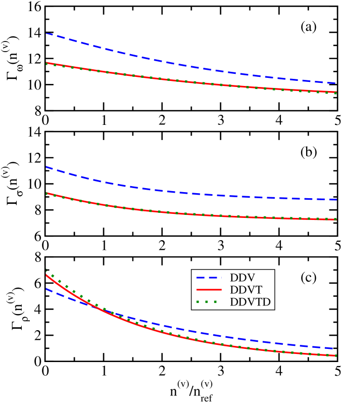
Figure 1: Coupling functions of the $\omega$ (a), $\sigma$ (b), and $\rho$ (c) meson for models with a vector density dependence.

The actual density dependence of the couplings is depicted in figures 1 and 2 for the cases of a vector or scalar density dependence, respectively. Only the $\omega$, $\sigma$ and $\rho$ couplings are shown because the $\delta$ coupling has the same shape as the $\rho$ coupling if it is nonzero. A typical decrease of the couplings with increasing density is observed. All couplings behave rather similarly. The $\rho$ meson coupling decreases more strongly than the $\omega$ and $\sigma$ couplings. It vanishes at infinitely high density because the exponential form (63) was chosen. The situation is different for the isoscalar mesons. They approach a nonzero finite value in this limit. The variations between the parametrisations are less strong for the $\rho$ meson as compared to the isoscalar mesons.

4.2 Uncertainties of observables

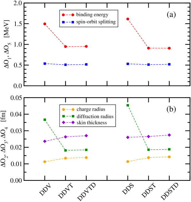
Figure 3: Uncertainties $\Delta O_{i}$ of the parametrisation in energy observables (a) and length observables (b).

The introduction of tensor couplings in the energy density functional also affects the uncertainties of nuclear observables that enter in the calculation of the $\chi^{2}$ function (66). They are given in table 3 and shown in figure 3. Most striking is the reduction of the uncertainty in the binding energies (upper panel) and in the diffraction radii (lower panel) when the tensor couplings are considered. In contrast, the charge radii and skin thicknesses are only described slightly worse than in the models without tensor interaction. Taking the $\delta$ meson into account does not make a big difference. The uncertainties of the spin-orbit splittings are almost the same for all models. The observed trends are very similar for models with a vector or a scalar density dependence of the couplings. Overall, terms with tensor couplings seem to be a valuable contribution in the EDF to improve the description of nuclear observables.

4.3 Nuclear matter parameters

With the fitted parameters of the energy density functionals, the characteristic parameters of nuclear matter can be calculated easily from the dependence of the energy density (2.3) on the baryon density $n_{b}$ and the isospin asymmetry $\delta$. They are given in tables 4 and 5 with uncertainties, including the $\sigma$ meson mass and the average Dirac effective mass $m^{\ast}=(m_{n}^{\ast}+m_{p}^{\ast})/2$ at saturation in symmetric nuclear matter.

The most notable result of including tensor couplings is the substantial rise of the Dirac effective mass at saturation and the drop in the mass of the $\sigma$ meson. At the same time the uncertainties of these two quantities rise in the parametrisations with tensor couplings. In conventional relativistic energy density functionals without tensor couplings the Dirac effective mass has to be rather small in order to find a reasonable size of spin-orbit splittings in nuclei. The proper binding energy per nucleon is primarily determined by the difference $V-S$ of the vector and scalar potentials whereas the spin-orbit splitting depends on the gradient of the sum $V+S$. Hence, in order to describe both observables reasonably well, strong constraints are put on the size of $V$ and $S$ themselves and thus on the couplings of the $\omega$ and $\sigma$ mesons. With tensor couplings, there is an additional contribution to the spin-orbit potential. The Dirac effective mass can be larger and the $\sigma$ meson coupling smaller than usual, cf. table 1. Since effects of the tensor couplings are related to the variation of the densities, it is of no surprise that other quantities that are sensitive to the description of the nuclear surface are also affected. This is particular true for the mass of the $\sigma$ meson because its low mass determines the range of the interaction.

Another effect of tensor couplings is the slight increase of the saturation density of nuclear matter, whereas the binding energy per nucleon is less affected as seen in table 4. These two quantities are rather well constrained in the fit as the small uncertainties show. The skewness $Q$, however, is varying strongly between the models and is rather unconstrained, even though large negative values are preferred.

The symmetry energy $J$ and its slope parameter $L$ are also influenced by the introduction of the tensor couplings as seen from table 5. Both values reduce, in particular the slope parameter, when tensor couplings are introduced. The uncertainty of $J$ is usually in the order of $7$% for the DDV and DDS models or below $4.5$% for the other parametrisations. The slope parameter $L$ is much less constrained with uncertainties around $30$%. The symmetry energy incompressibilities $K_{\rm sym}$ are always found to be negative with values correlated to $J$ and $L$. The (negative) values of $K_{\tau,v}$ vary over a much larger range. In both cases the uncertainties are much larger for parametrisations with a scalar density dependence of the couplings.

4.4 Equation of state and symmetry energy

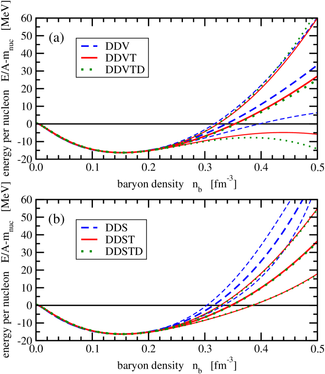
Figure 4: Equation of state of symmetric nuclear matter with coupling functions depending on the vector density (a) and on the scalar density (b). See text for details.

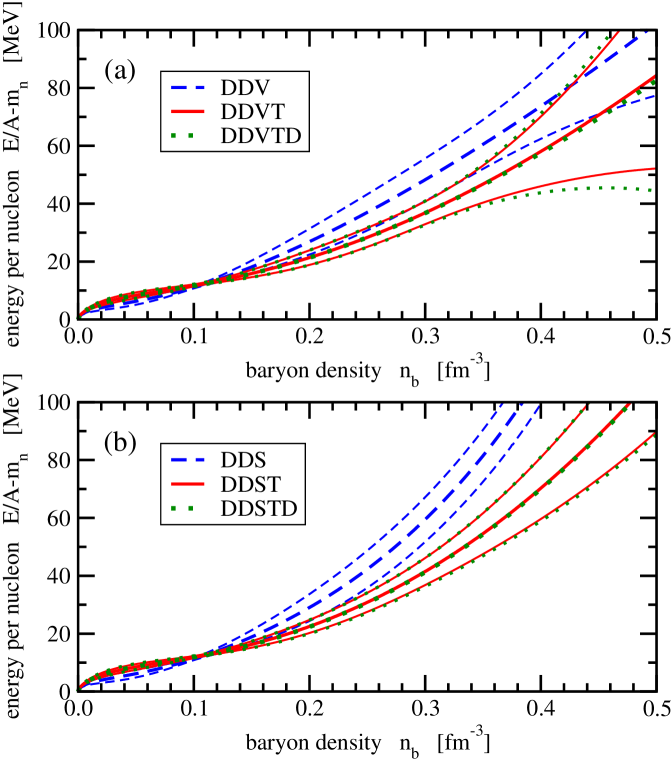
Figure 5: Equation of state of pure neutron matter with coupling functions depending on the vector density (a) and on the scalar density (b). See text for details.

The nuclear matter parameters characterise the equation of state (EoS) only close to saturation density and isospin asymmetry zero. A larger range of baryon densities is explored in figures 4 and 5 for symmetric nuclear matter and pure neutron matter, respectively. The results of the calculations with the best parameters are depicted with thick lines or dots. The uncertainty band is given by the corresponding thin lines and small dots with the same colors. There is hardly any difference between the models for the energy per nucleon up to nuclear saturation density. Different trends are seen at higher densities. This is obvious because the fit of the models to observables of nuclei is sensitive essentially only to the sub-saturation region as higher densities are not found in finite nuclei.

The models with a vector density dependence of the couplings (upper panel of figure 4) behave very similarly in the case of symmetric nuclear matter with a slight reduction of the stiffness when tensor couplings are included in the model. The ordering is similar in case of pure neutron matter (upper panel of figure 5) but the effect of softening is a bit stronger.

The situation is different for models with a scalar density dependence. Here, the models DDST and DDSTD are almost identical and much softer than the other two parametrisations. This is true for symmetric nuclear matter as well as pure neutron matter. The EoS of model DDS is stiffer at high densities than that of DDV, both without tensor interaction. A similar trend is observed for models with tensor interaction. This feature will be explained below when the evolution of effective masses and scalar densities is studied.

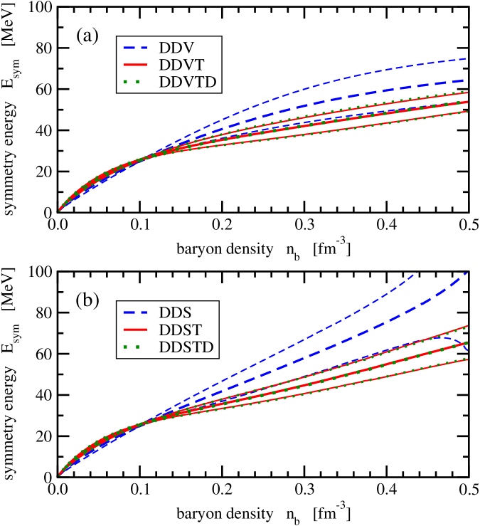
Figure 6: Symmetry energy as a function of the baryon density with coupling functions depending on the vector density (a) and on the scalar density (b). See text for details.

The density dependence of the nuclear symmetry calculated according to (56) is shown in figure 6, again for models with vector density dependence (upper panel) and scalar density dependence (lower panel). For baryon densities below saturation there is no big difference between the parametrisations as expected. At higher densities similar effects as in symmetric nuclear matter and pure neutron matter are seen with a strong stiffening for the models with a scalar density dependence. At a density of $n_{b}\approx 0.11$ fm^-3 all curves of the symmetry energy cross close to a single point and the uncertainty band is most narrow. A similar feature was seen already for the EoS of pure neutron matter. This particular density marks the density of highest sensitivity in nuclei that is below the saturation density of nuclear matter. This crossing of EoS was already observed very early on for Skyrme models Brown:2000pd .

Taking the $\delta$ meson into account in the parametrisations has almost no effect on the EoS of symmetric or pure nucleon matter and the density dependence of the symmetry energy.

4.5 Dirac effective masses and scalar densities

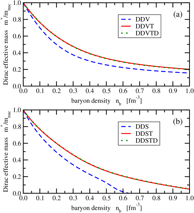
Figure 7: Dirac effective mass in symmetric nuclear matter as a function of the baryon density with coupling functions depending on the vector density (a) and on the scalar density (b).

The Dirac effective masses $m^{\ast}_{\rm nuc}$ of the nucleons in symmetric nuclear matter and pure neutron matter are depicted in figures 7 and 8, respectively. They decrease with increasing baryon density due to the increase of the scalar potential. The effective masses in pure neutron matter are generally lower than those in symmetric nuclear matter. The models DDVT, DDVTD, DDST, and DDSTD show a larger effective mass than the DDV and DDS models, respectively, throughout the covered range of baryon densities in the figures. The scalar potential $S$ has to be less strong to obtain the spin-orbit splitting in nuclei because the tensor couplings give an additional contribution.

The models with scalar density dependence of the couplings exhibit the peculiar feature that the Dirac effective mass vanishes at some density above saturation. At that point the scalar potential $S_{i}$ of a nucleon $i$ reaches the vacuum nucleon mass $m_{i}$. This can happen only because the rearrangement contribution from the $\omega$ meson coupling in (2.1) increases without bounds for a negative derivative $d\Gamma{\omega}/dn^{(s)}$ of the $\omega$ coupling function. The effect is more pronounced for pure neutron matter than for symmetric nuclear matter with lower collapse densities.

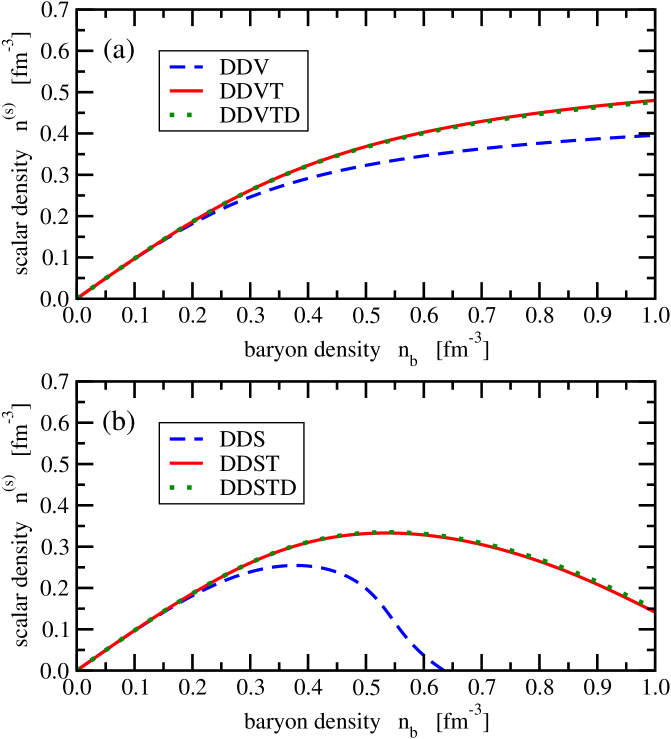
Figure 9: Scalar density in symmetric nuclear matter as a function of the baryon density with coupling functions depending on the vector density (a) and on the scalar density (b).

The behaviour of the Dirac effective masses is correlated with vanishing scalar densities at a certain baryon density above saturation, as depicted in figures 9 and 10. In the case of models with couplings that depend on the vector density, there is a smooth and continuous rise of the scalar densities with decreasing slope (upper panels). In contrast, the scalar density in the models with scalar density dependent couplings first rise and then decline reaching zero eventually (lower panels).

The decrease of the effective masses and scalar densities at high densities for the models with a scalar density dependence of the couplings modifies the kinetic contributions (48) to the pressure of the system. In other models, the decline of $m_{i}^{\ast}$ with baryon density is partly compensated by a rise of $n_{i}^{(s)}$. In contrast, the product $m_{i}^{\ast}n_{i}^{(s)}$ in models with couplings of scalar density dependence reduces much faster at higher baryon densities and a stiffer EoS is expected as confirmed in figures (4) and (5).

5 Conclusions

The construction of energy density functionals resulting from relativistic mean-field models leaves ample room for variations. In this work two main aspects of the form of the EDF were studied in more detail: the dependence of the minimal nucleon-meson couplings on the total Lorentz vector or scalar density of the system and the effects of tensor couplings of the isovector mesons with the nucleons. Furthermore, the effect of including the $\delta$ meson in addition to the standard isovector $\rho$ meson is explored.

Since relativistic EDFs are phenomenological descriptions of finite nuclei and nuclear matter depending on a certain number of parameters, these quantities, which determine the effective in-medium interaction, cannot be related directly to the free nucleon-nucleon interaction that is well constrained by scattering data. Instead, the model parameters have to be found by a fit to nuclear observables. Contrary to most earlier approaches, a self-consistent determination of the uncertainties in the $\chi^{2}$ function was realized in this work leading to more realistic values than from heuristic estimates.

The main results of this work can be summarized as follows. The inclusion of tensor couplings in the relativistic EDF reduces the strength of the isoscalar minimal nucleon-meson couplings as compared to models without tensor couplings. For all mesons a reduction of the couplings with increasing baryon density is found in all cases. The description of finite nuclei improves with tensor couplings, in particular for the binding energies and diffraction radii. The equation of state of nuclear matter is very similar for all models at sub-saturation densities. The characteristic nuclear matter parameters at saturation and the parameters of the EDFs exhibit some correlation with the choice of the density dependence of the couplings and the inclusion of the tensor couplings or not. Saturation densities, binding energies at saturation, symmetry energies and slope parameters of the models are rather well constrained. Higher-order derivatives show much larger uncertainties. At high densities large variations of the predictions of the EoS are observed with a substantial increase of the model uncertainties. The lowest uncertainties are found close to a density of about $0.11$ fm^-3 where all EoSs cross close to a single point. Models with a scalar density dependence are stiffer at high densities than models with a vector density dependence of the couplings. This observation is related to the collapse of the total scalar density of the system and vanishing effective mass at high baryon densities in approaches with couplings depending on scalar densities. The rearrangement contribution from the dependence of the $\omega$ coupling on the scalar density leads to an unlimited increase of the scalar potential in this case. Models with tensor couplings have larger effective nucleon masses than models without. This is possible because the tensor contributions increase the spin-orbit splitting so that a smaller strength of the Lorentz scalar $\sigma$ meson is needed to fit the nuclear data.

In order to avoid the problems with the scalar density dependence of all couplings, a change to a mixed density dependence can be considered, i.e. a dependence of Lorentz vector meson couplings on the vector density and Lorentz scalar meson couplings on the scalar density. Models of this type have been explored in Typel:2018cap but without tensor couplings and without a self-consistent determination of the uncertainties of the fitted observables. Work in this direction is in progress using an extended set of nuclei and more observables in the fitting procedure.

Another aspect is also worthwhile to be investigated further. In the present approach, the incompressibility of nuclear matter was kept to a fixed value because a fit to only ground state properties of finite nuclei does not help to fix this quantity very well. Properties of excited states like giant resonances, in particular the isoscalar giant monopole resonance, have to be included in the fitting procedure and can help much better to find proper values of $K$, see, e.g., Shlomo:2019bgh . The study of other types of giant resonances that constrain the isovector part of the effective interaction will also be useful.

In general, a better description of surface properties of finite nuclei will be very rewarding by considering appropriately chosen new terms in the EDF. It is known that the incompressibility of nuclear matter is closely related to the surface thickness and surface tension as expressed by the so-called pocket formula Stocker:1980olw ; Brack:1982yki . More precise experimental data on the neutron skin thickness would help to determine the isovector parts of the EDF more precisely.

6 Acknowledgements

Discussions with Daniel R. Phillips, Shalom Shlomo, and Dario Vretenar are acknowledged. This work was initiated during a two-month visit of DAT at the Institut für Kernphysik in Darmstadt which was supported by an Erasmus+ traineeship.

Appendix A

The rearrangement contributions (2.1) and (2.1) to the vector and scalar potentials (13) and (14), respectively, arise from the density dependence of the couplings $\tilde{\Gamma}_{j}$ in the covariant derivative (3) and the effective mass operator (4) when the field equation of the nucleons is deduced with the help of the Euler-Langrange equation

$$0=\frac{\partial\mathcal{L}}{\partial\overline{\Psi}_{ik}}-\partial_{\nu}\frac{\partial\mathcal{L}}{\partial(\partial_{\nu}\overline{\Psi}_{ik})}$$ (72)

with the Lagrangian density (1). Here the indices $i$ and $k$ are used with $i$ distinguishing between protons and neutrons and $k$ to identify a particular single-particle state. Hence the nucleonic contribution to $\mathcal{L}$ reads

$$\mathcal{L}_{\rm nucleon}$$

$$= \sum_{i=p,n}\sum_{k}w_{ik}\overline{\Psi}_{ik}\left(\gamma_{\mu}iD_{ik}^{\mu}-\sigma_{\mu\nu}T_{ik}^{\mu\nu}-M_{ik}^{\ast}\right)\Psi_{ik}$$

if the occupation factors $w_{ik}=0$ or $1$ are introduced similar as in the definitions (9) and (10) of the current and scalar density. Since $\mathcal{L}$ does not depend on derivatives of $\overline{\Psi}_{ik}$ only the first term in (72) remains. The result

$$0=w_{ik}\left(\gamma_{\mu}iD_{ik}^{\mu}-\sigma_{\mu\nu}T_{ik}^{\mu\nu}-M_{ik}^{\ast}\right)\Psi_{ik}$$

$$-\sum_{i^{\prime}=p,n}\sum_{k^{\prime}}w_{i^{\prime}k^{\prime}}\overline{\Psi}_{i^{\prime}k^{\prime}}\gamma_{\mu}\left(\frac{\partial\tilde{\Gamma}_{\omega}}{\partial\overline{\Psi}_{ik}}\omega^{\mu}+\frac{\partial\tilde{\Gamma}_{\varrho}}{\partial\overline{\Psi}_{ik}}\vec{\varrho}^{\mu}\cdot\vec{\tau}\right)\Psi_{i^{\prime}k^{\prime}}$$

$$+\sum_{i^{\prime}=p,n}\sum_{k^{\prime}}w_{i^{\prime}k^{\prime}}\overline{\Psi}_{i^{\prime}k^{\prime}}\left(\frac{\partial\tilde{\Gamma}_{\sigma}}{\partial\overline{\Psi}_{ik}}\sigma+\frac{\partial\tilde{\Gamma}_{\delta}}{\partial\overline{\Psi}_{ik}}\vec{\delta}\cdot\vec{\tau}\right)\Psi_{i^{\prime}k^{\prime}}$$

contains in the first line the usual form of the Dirac equation for nucleon $k$. The dependence of the couplings $\tilde{\Gamma}_{j}$ on the nucleon fields leads to the contributions in the second and third line. Assuming a dependence on the vector density $\rho_{v}$ or the scalar density $\rho_{s}$, the expression

$$\frac{\partial\tilde{\Gamma}_{j}}{\partial\overline{\Psi}_{ik}} = \frac{\partial\tilde{\Gamma}_{j}}{\partial\rho_{v}}\frac{\partial\rho_{v}}{\partial\overline{\Psi}_{ik}}+\frac{\partial\tilde{\Gamma}_{j}}{\partial\rho_{s}}\frac{\partial\rho_{s}}{\partial\overline{\Psi}_{ik}}$$

$$= \frac{\partial\tilde{\Gamma}_{j}}{\partial\rho_{v}}\frac{j^{\mu}}{\rho_{v}}\gamma_{\mu}w_{ik}\Psi_{ik}+\frac{\partial\tilde{\Gamma}_{j}}{\partial\rho_{s}}w_{ik}\Psi_{ik}$$

is found with equations (9) and (10). The equation (Appendix A) becomes

$$0 = \gamma_{\mu}\left(i\partial^{\mu}-\tilde{\Gamma}_{\omega}\omega^{\mu}-\tilde{\Gamma}_{\rho}\vec{\rho}^{\mu}\cdot\vec{\tau}-\Gamma_{\gamma}A^{\mu}\frac{1+\tau_{3}}{2}\right)\Psi_{ik}$$

$$-\left(m_{i}-\tilde{\Gamma}_{\sigma}\sigma-\tilde{\Gamma}_{\delta}\vec{\delta}\cdot\vec{\tau}\right)\Psi_{ik}$$

$$-\left(\frac{\partial\tilde{\Gamma}_{\omega}}{\partial\rho_{v}}\frac{j^{\mu}}{\rho_{v}}\gamma_{\mu}+\frac{\partial\tilde{\Gamma}_{\omega}}{\partial\rho_{s}}\right)\Psi_{ik}\omega^{\nu}\sum_{i^{\prime}=p,n}\sum_{k^{\prime}}\overline{\Psi}_{i^{\prime}k^{\prime}}\gamma_{\nu}\Psi_{i^{\prime}k^{\prime}}$$

$$-\left(\frac{\partial\tilde{\Gamma}_{\rho}}{\partial\rho_{v}}\frac{j^{\mu}}{\rho_{v}}\gamma_{\mu}+\frac{\partial\tilde{\Gamma}_{\rho}}{\partial\rho_{s}}\right)\Psi_{ik}\vec{\varrho}^{\nu}\cdot\sum_{i^{\prime}=p,n}\sum_{k^{\prime}}\overline{\Psi}_{i^{\prime}k^{\prime}}\gamma_{\nu}\vec{\tau}\Psi_{i^{\prime}k^{\prime}}$$

$$+\left(\frac{\partial\tilde{\Gamma}_{\sigma}}{\partial\rho_{v}}\frac{j^{\mu}}{\rho_{v}}\gamma_{\mu}+\frac{\partial\tilde{\Gamma}_{\sigma}}{\partial\rho_{s}}\right)\Psi_{ik}\sigma\sum_{i^{\prime}=p,n}\sum_{k^{\prime}}\overline{\Psi}_{i^{\prime}k^{\prime}}\Psi_{i^{\prime}k^{\prime}}$$

$$+\left(\frac{\partial\tilde{\Gamma}_{\delta}}{\partial\rho_{v}}\frac{j^{\mu}}{\rho_{v}}\gamma_{\mu}+\frac{\partial\tilde{\Gamma}_{\delta}}{\partial\rho_{s}}\right)\Psi_{ik}\vec{\delta}\cdot\sum_{i^{\prime}=p,n}\sum_{k^{\prime}}\overline{\Psi}_{i^{\prime}k^{\prime}}\vec{\tau}\Psi_{i^{\prime}k^{\prime}}$$

$$-\sigma_{\mu\nu}T_{i}^{\mu\nu}\Psi_{ik}$$

where the source currents and densities

$$j_{\omega\mu} = \sum_{i^{\prime}=p,n}\sum_{k^{\prime}}w_{i^{\prime}k^{\prime}}\overline{\Psi}_{i^{\prime}k^{\prime}}\gamma_{\mu}\Psi_{i^{\prime}k^{\prime}}$$ (77)

$$\vec{j}_{\rho\mu} = \sum_{i^{\prime}=p,n}\sum_{k^{\prime}}w_{i^{\prime}k^{\prime}}\overline{\Psi}_{i^{\prime}k^{\prime}}\gamma_{\mu}\vec{\tau}\Psi_{i^{\prime}k^{\prime}}$$ (78)

$$\varrho_{\sigma} = \sum_{i^{\prime}=p,n}\sum_{k^{\prime}}w_{i^{\prime}k^{\prime}}\overline{\Psi}_{i^{\prime}k^{\prime}}\Psi_{i^{\prime}k^{\prime}}$$ (79)

$$\vec{\varrho}_{\delta} = \sum_{i^{\prime}=p,n}\sum_{k^{\prime}}w_{i^{\prime}k^{\prime}}\overline{\Psi}_{i^{\prime}k^{\prime}}\vec{\tau}\Psi_{i^{\prime}k^{\prime}}$$ (80)

are easily identified. Reordering the contributions gives

$$0 = \left[\gamma_{\mu}\left(i\partial^{\mu}-\Sigma^{\mu}\right)-\sigma_{\mu\nu}T_{i}^{\mu\nu}-\left(m_{i}-\Sigma\right)\right]\Psi_{ik}$$ (81)

with the explicit forms of the scalar self-energy

$$\Sigma = \tilde{\Gamma}_{\sigma}\sigma+\frac{\partial\tilde{\Gamma}_{\sigma}}{\partial\rho_{s}}\sigma\varrho_{\sigma}+\tilde{\Gamma}_{\delta}\vec{\delta}\cdot\vec{\tau}+\frac{\partial\tilde{\Gamma}_{\delta}}{\partial\rho_{s}}\vec{\delta}\cdot\vec{\varrho}_{\delta}$$

$$-\frac{\partial\tilde{\Gamma}_{\omega}}{\partial\rho_{s}}\omega^{\nu}j_{\omega\nu}-\frac{\partial\tilde{\Gamma}_{\rho}}{\partial\rho_{s}}\vec{\varrho}^{\nu}\cdot\vec{j}_{\rho\nu}$$

and the vector self-energy

$$\Sigma^{\mu} = \tilde{\Gamma}_{\omega}\omega^{\mu}+\frac{\partial\tilde{\Gamma}_{\omega}}{\partial\rho_{v}}\frac{j^{\mu}}{\rho_{v}}\omega^{\nu}j_{\omega\nu}+\tilde{\Gamma}_{\rho}\vec{\rho}^{\mu}\cdot\vec{\tau}+\frac{\partial\tilde{\Gamma}_{\rho}}{\partial\rho_{v}}\frac{j^{\mu}}{\rho_{v}}$$

$$-\frac{\partial\tilde{\Gamma}_{\sigma}}{\partial\rho_{v}}\frac{j^{\mu}}{\rho_{v}}\sigma\varrho_{\sigma}-\frac{\partial\tilde{\Gamma}_{\delta}}{\partial\rho_{v}}\frac{j^{\mu}}{\rho_{v}}\vec{\delta}\cdot\vec{\varrho}_{\delta}+\Gamma_{\gamma}A^{\mu}\frac{1+\tau_{3}}{2}\>.$$

In the mean-field approximation and under the symmetries of the application to spherical nuclei, the currents and densities (77), (78), (79), and (80) reduce to the forms (34) and (35) with the appropriate coupling factors $g_{ij}$. Similarly, the self-energies (Appendix A) and (Appendix A) become simple potentials (13) and (14) where only the $\mu=0$ component of $\Sigma^{\mu}$ and $j^{0}=\rho_{v}$ remain. The rearrangement contributions (2.1) and (2.1) are easily recognized when the functionals $\tilde{\Gamma}_{j}$ of the fields are replaced by functions $\Gamma_{j}$ of the densities.

Appendix B

The energy density functional (2.3) contains in total $19$ parameters: the masses of nucleons and mesons (six), the reference density (one) and the nucleon-meson couplings at this density (four), the parameters describing the density dependence of the couplings (six), and the tensor couplings (two). However, really used are only $14$ because the masses of the nucleons and mesons, except for the $\sigma$ meson, are kept constant. Thus there are eight parameters for the isoscalar part of the effective interaction and six for the isovector part.

In the actual fitting procedure six of the eight isoscalar parameters are replaced by four characteristic parameters of symmetric nuclear matter and two auxiliary quantities. The mass of the sigma meson $m_{\sigma}$ and the $\omega$ tensor coupling $\Gamma_{T\omega}$ are used directly as independent quantities. The four nuclear matter parameters are the saturation density $n_{\rm sat}$, the Dirac effective mass $m^{\ast}_{\rm sat}$ at saturation, the binding energy per nucleon at saturation $B_{\rm sat}$ and the incompressibility $K$. The two auxiliary quantities are the derivative $f_{\omega}^{\prime}(1)$ and the ratio $r=f_{\omega}^{\prime\prime}(1)/f_{\omega}^{\prime}(1)$ of derivatives. The transformation proceeds in two steps. First, the nuclear matter parameters are converted to the coupling factors $C_{j}=\Gamma_{j}^{2}/m_{j}^{2}$ for $j=\omega,\sigma$, their first derivatives $D_{j}^{(v)}$ or $D_{j}^{(s)}$ and second derivatives $E_{j}^{(v)}$ or $E_{j}^{(s)}$ as defined in subsection 2.3. Then these quantities are used to calculated the parameters $a_{j}$, $b_{j}$, $c_{j}$, and $d_{j}$ of the rational function (62).

In the parameter conversion, the average nucleon mass $m_{\rm nuc}=(m_{p}+m_{n})/2$ is used and the real nuclear matter parameters are calculated numerically at the end of the fitting procedure with the correct nucleon masses to be independent of this averaging.

The saturation density $n_{\rm sat}$ defines the Fermi momentum

$$p_{\rm sat}^{\ast}=\left(\frac{3\pi^{2}}{2}n_{\rm sat}\right)^{\frac{1}{3}}$$ (84)

in symmetric nuclear matter. With the Dirac effective mass $m_{\rm sat}^{\ast}$ the effective chemical potential

$$\mu_{\rm sat}^{\ast}=\sqrt{(p_{\rm sat}^{\ast})^{2}+(m_{\rm sat}^{\ast})^{2}}$$ (85)

and the corresponding scalar density

$$n_{\rm sat}^{(s)}=\frac{m_{\rm sat}^{\ast}}{\pi^{2}}\left[p_{\rm sat}^{\ast}\mu_{\rm sat}^{\ast}-\left(m_{\rm sat}^{\ast}\right)^{2}\ln\frac{p_{\rm sat}^{\ast}+\mu_{\rm sat}^{\ast}}{m_{\rm sat}^{\ast}}\right]$$ (86)

at saturation are given. The saturation density $n_{\rm sat}$ or the scalar density at saturation $n_{\rm sat}^{(s)}$ are used as the reference density $n_{\rm ref}$ in the coupling functions if a vector or scalar density dependence is selected, respectively. Then the scalar and vector potential at saturation are found as

$$S_{\rm sat}=m_{\rm nuc}-m_{\rm sat}^{\ast}$$ (87)

and

$$V_{\rm sat}=m_{\rm nuc}-B_{\rm sat}-\mu_{\rm sat}^{\ast}$$ (88)

with the binding energy per nucleon $B_{\rm sat}$. Furthermore the factor (54) at saturation

$$f_{\rm sat}=3\left(\frac{n_{\rm sat}^{(s)}}{m_{\rm sat}^{\ast}}-\frac{n_{\rm sat}}{\mu_{\rm sat}^{\ast}}\right)$$ (89)

is defined for later convenience. For the next step one has to distinguish the type of density dependence.

In case of a vector density dependence with $n_{\rm ref}=n_{\rm sat}^{(v)}$ there is no rearrangement contribution to the scalar potential, $S_{\rm sat}^{(R)}=0$, and the $\sigma$ coupling

$$C_{\sigma}(n_{\rm ref})=\frac{\Gamma_{\sigma}^{2}(n_{\rm ref})}{m_{\sigma}^{2}}=\frac{S_{\rm sat}}{n_{\rm sat}^{(s)}}$$ (90)

and thus $\Gamma_{\sigma}(n_{\rm ref})$ for given $m_{\sigma}$ are immediately obtained. The vector coupling is found with (2.3) to be

$$C_{\omega}(n_{\rm ref}) = \frac{\Gamma_{\omega}^{2}(n_{\rm ref})}{m_{\omega}^{2}}$$

$$= \frac{2}{n_{\rm sat}^{2}}\left[\left(m_{\rm nuc}-B_{\rm sat}\right)n_{\rm sat}-\frac{1}{2}C_{\sigma}\left(n_{\rm sat}^{(s)}\right)^{2}\right.$$

$$\left.-\frac{1}{4}\left(3\mu_{\rm sat}^{\ast}n_{\rm sat}+m_{\rm sat}^{\ast}n_{\rm sat}^{\ast}\right)\right]$$

in symmetric nuclear matter. Then the rearrangement contribution to $V_{\rm sat}$ is

$$V_{\rm sat}^{(R)}=V_{\rm sat}-C_{\omega}\left(n_{\rm sat}^{(v)}\right)^{2}$$ (92)

and the derivatives

$$D_{\omega}^{(v)}(n_{\rm ref})=2f_{\omega}^{\prime}(1)\frac{C_{\omega}}{n_{\rm sat}^{(v)}}$$ (93)

and

$$D_{\sigma}^{(v)}(n_{\rm ref})=\frac{D_{\omega}^{(v)}\left(n_{\rm ref}\right)^{2}-2V_{\rm sat}^{(R)}}{\left(n_{\rm sat}^{(s)}\right)^{2}}$$ (94)

are determined with the auxiliary quantity $f_{\omega}^{\prime}(1)$. Defining

$$E_{\omega}^{(v)}(n_{\rm ref})=\frac{2C_{\omega}}{(n_{\rm sat}^{(v)})^{2}}f_{\omega}^{\prime}(1)\left[f_{\omega}^{\prime}(1)+r\right]$$ (95)

and

$$g_{\rm sat}^{(v)}=\frac{\frac{m_{\rm sat}^{\ast}}{\mu_{\rm sat}^{\ast}}-f_{\rm sat}D_{\sigma}^{(v)}n_{\rm sat}^{(s)}}{1+f_{\rm sat}C_{\sigma}}$$ (96)

the second derivative

$$E_{\sigma}^{(v)}(n_{\rm ref})=$$

$$\left[3\left(\mu_{\rm sat}^{\ast}-m_{\rm sat}^{\ast}g_{\rm sat}^{(v)}\right)-K\right.$$

$$+9C_{\omega}n_{\rm sat}^{(v)}+18D_{\omega}^{(v)}(n_{\rm sat}^{(v)})^{2}+\frac{9}{2}E_{\omega}^{(v)}(n_{\rm sat}^{(v)})^{3}$$

$$\left.-9D_{\sigma}^{(v)}\left(n_{\rm sat}^{(s)}\right)^{2}-9\left(C_{\sigma}+D_{\sigma}^{(v)}n_{\rm sat}^{(v)}\right)n_{\rm sat}^{(s)}g_{\rm sat}^{(v)}\right]$$

$$\left[\frac{9}{2}n_{\rm sat}^{(v)}\left(n_{\rm sat}^{(s)}\right)^{2}\right]^{-1}$$

is found from the incompressibility $K$ using (52) and (2.3).

The calculation proceeds slightly differently in case of couplings that depend of the scalar density. It is more complicated because both expressions (52) and (2.3) depend explicitly on the second derivatives of the couplings. Since the rearrangement contribution $V_{\rm sat}^{(R)}$ is zero, the $\omega$ coupling

$$C_{\omega}(n_{\rm ref})=\frac{\Gamma_{\omega}^{2}(n_{\rm ref})}{m_{\omega}^{2}}=\frac{V_{\rm sat}}{n_{\rm sat}^{(v)}}$$ (98)

is directly found as well as the derivatives

$$D_{\omega}^{(v)}(n_{\rm ref})=2f_{\omega}^{\prime}(1)\frac{C_{\omega}}{n_{\rm ref}}$$ (99)

and

$$E_{\omega}^{(v)}(n_{\rm ref})=\frac{2C_{\omega}}{n_{\rm ref}^{2}}f_{\omega}^{\prime}(1)\left[f_{\omega}^{\prime}(1)+r\right]$$ (100)

where the reference density $n_{\rm ref}$ is now identical to the scalar density $n_{\rm sat}^{(s)}$. The rearrangement contribution to the scalar potential is

$$S_{\rm sat}^{(R)} = \frac{1}{n_{\rm sat}^{(s)}}\left(\frac{1}{2}\mu_{\rm sat}^{\ast}n_{\rm sat}^{(v)}-\frac{1}{2}m_{\rm sat}^{\ast}n_{\rm sat}^{(s)}\right.$$

$$\left.+V_{\rm sat}n_{\rm sat}^{(v)}-S_{\rm sat}n_{\rm sat}^{(s)}\right)$$

because the pressure (47) is zero at the saturation density. If one defines the auxiliary quantity

$$X_{\rm sat}=\frac{Y_{\rm sat}}{Z_{\rm sat}}$$ (102)

as the ratio of

$$Y_{\rm sat} = \left(\frac{m_{\rm sat}^{\ast}}{\mu_{\rm sat}^{\ast}}+f_{\rm sat}D_{\omega}^{(s)}n_{\rm sat}^{(v)}\right)$$

$$\left(C_{\sigma}n_{\rm sat}^{(s)}+2D_{\sigma}^{(s)}(n_{\rm sat}^{(s)})^{2}-D_{\omega}^{(s)}(n_{\rm sat}^{(v)})^{2}+\frac{m_{\rm sat}^{\ast}}{3}\right)$$

$$-\left[1+f_{\rm sat}\left(C_{\sigma}+2D_{\sigma}^{(s)}n_{\rm sat}^{(s)}\right)\right]$$

$$\left[\frac{\mu_{\rm sat}^{\ast}}{3}-\frac{K}{9}+\left(C_{\omega}+D_{\omega}^{(s)}n_{\rm sat}^{(s)}\right)n_{\rm sat}^{(v)}\right]$$

and

$$Z_{\rm sat}=f_{\rm sat}\left(\frac{\mu_{\rm sat}^{\ast}}{3}-\frac{K}{9}+C_{\omega}n_{\rm sat}^{(v)}\right)-n_{\rm sat}^{(s)}\frac{m_{\rm sat}^{\ast}}{\mu_{\rm sat}^{\ast}}$$ (104)

then the second derivative $E_{\sigma}^{(s)}(n_{\rm ref})$ is easily obtained from

$$E_{\sigma}^{(s)}=\frac{1}{(n_{\rm sat}^{(s)})^{2}}\left[2X_{\rm sat}+E_{\omega}^{(s)}(n_{\rm sat}^{(v)})^{2}\right]\>.$$ (105)

In the next step of the parameter conversion, the couplings $C_{\sigma}$ and their derivatives are used to define the function derivatives

$$f_{\sigma}^{\prime}(1)=\frac{D_{\sigma}^{(x)}n_{\rm sat}^{(x)}}{2C_{\sigma}}$$ (106)

and

$$f_{\sigma}^{\prime\prime}(1)=\frac{E_{\sigma}^{(x)}(n_{\rm sat}^{(x)})^{2}}{2C_{\sigma}}-\left[f_{\sigma}^{\prime}(1)\right]^{2}$$ (107)

where $x=v$ or $s$ depending on the type of density dependence. The corresponding values $f_{\omega}^{\prime}(1)$ and $f_{\omega}^{\prime\prime}(1)$ are already known because they were used as original parameters in the fit.

Finally the quantities $f_{j}^{\prime}(1)$ and $f_{j}^{\prime\prime}(1)$ for $j=\omega$ and $\sigma$ are used to determine the actual parameters of the rational function (62). For this purpose, the first and second derivatives of the function (62) are needed. They are given by

$$f_{j}^{\prime}(x)=2a_{j}(b_{j}-c_{j})\frac{(x+d_{j})}{\left[1+c_{j}(x+d_{j})^{2}\right]^{2}}$$ (108)

and

$$f_{j}^{\prime\prime}(x)=2a_{j}(b_{j}-c_{j})\frac{1-3c_{j}(x+d_{j})^{2}}{\left[1+c_{j}(x+d_{j})^{2}\right]^{3}}$$ (109)

where the condition $f_{j}^{\prime\prime}(0)=0$ leads to the condition $c_{j}=1/(3d_{j}^{2})$. With the known ratio

$$R_{21}(d_{j})=\frac{f_{j}^{\prime\prime}(1)}{f_{j}^{\prime}(1)} = \frac{1-3c_{j}(1+d_{j})^{2}}{\left[1+c_{j}(1+d_{j})^{2}\right](1+d_{j})}$$

$$= \frac{-1-2d_{j}}{\left[d_{j}^{2}+\frac{1}{3}(1+d_{j})^{2}\right](1+d_{j})}$$

an equation to determine $d_{j}$ is obtained. The function $R_{21}(d_{j})$ is negative for $d_{j}>-1/2$. A unique solution with positive $d_{j}$ is possible for $-3\leq R_{21}<0$. Only this branch is considered in the present parameter fits. With the known $d_{j}$ and then $c_{j}$, the parameter $b_{j}$ is found from the ratio

$$R_{10}(d_{j}) = \frac{f_{j}^{\prime}(1)}{f_{j}(1)}$$

$$= \frac{2(b_{j}-c_{j})(1+d_{j})}{[1+c_{j}(1+d_{j})^{2}][1+b_{j}(1+d_{j})^{2}]}$$

as

$$b_{j}=\frac{R_{10}+c_{j}S}{S-R_{10}(1+d_{j})^{2}}$$ (112)

with the auxiliary quantity

$$S=\frac{2(1+d_{j})}{1+c_{j}(1+d_{j})^{2}}\>.$$ (113)

Finally, the parameter $a_{j}$ is found from the normalisation condition $f_{j}(1)=1$ as

$$a_{j}=\frac{1+c_{j}(1+d_{j})^{2}}{1+b_{j}(1+d_{j})^{2}}\>.$$ (114)

Table 1: Mass of the $\sigma$ meson and coupling strengths at the reference density for the different parametrisations.

parametrisation	number of	mass of	$\omega$ meson	$\sigma$ meson	$\rho$ meson	$\delta$ meson	$\omega$ tensor	$\rho$ tensor
	parameters	$\sigma$ meson	coupling	coupling	coupling	coupling	coupling	coupling
		$m_{\sigma}$	$\Gamma_{\omega}^{(0)}$	$\Gamma_{\sigma}^{(0)}$	$\Gamma_{\rho}^{(0)}$	$\Gamma_{\delta}^{(0)}$	$\Gamma_{T\omega}$	$\Gamma_{T\rho}$
	$N_{\rm par}$	[MeV]
DDV	8	537.600098	12.770450	10.136960	3.9241650	0.0000000	0.000000	0.0000000
DDVT	10	502.598602	10.987106	8.382863	3.8485560	0.0000000	3.681512	12.608333
DDVTD	11	502.619843	10.980433	8.379269	4.0301900	0.8487420	3.671994	12.382725
DDS	8	539.257996	12.925653	10.272845	3.9619391	0.0000000	0.000000	0.0000000
DDST	10	506.451447	11.170835	8.556703	3.8558209	0.0000000	3.869954	12.601035
DDSTD	11	505.835999	11.138900	8.526903	4.0612888	1.7924930	3.938227	12.087422

Table 2: Parameters for the density dependence of couplings. The coefficients $d_{j}$ for $j=\omega,\sigma$ are given by $d_{j}=1/\sqrt{3c_{j}}$, except for $d_{\omega}=3758.39866319$ in case of DDSTD.

parametrisation	$n_{\rm ref}^{(v)}$	$n_{\rm ref}^{(s)}$	$b_{\omega}$	$c_{\omega}$	$b_{\sigma}$	$c_{\sigma}$	$a_{\rho}=a_{\delta}$
DDV	0.151117	0.14218170	0.03911422	0.07239939	0.21286844	0.30798197	0.35265899
DDVT	0.153623	0.14636172	0.04459850	0.06721759	0.19210314	0.27773566	0.54870200
DDVTD	0.153636	0.14637920	0.02640016	0.04233010	0.19171263	0.27376859	0.55795902
DDS	0.151186	0.14218154	0.03643847	0.08348558	0.13985555	0.23568086	0.34219700
DDST	0.153923	0.14673361	$-3.786315\cdot 10^{-5}$	$1.611143\cdot 10^{-5}$	0.13972293	0.20737662	0.56369799
DDSTD	0.153999	0.14683193	$-7.009164\cdot 10^{-8}$	0.00000000	0.14036291	0.20810260	0.58325702

Table 3: Uncertainties of the observables used in the fitting of the parametrisations.

parametrisation	binding	charge	diffraction	surface	spin-orbit
	energy	radius	radius	thickness	splitting
	uncertainty	uncertainty	uncertainty	uncertainty	uncertainty
	$\Delta O_{1}$	$\Delta O_{2}$	$\Delta O_{3}$	$\Delta O_{4}$	$\Delta O_{5}$
	[MeV]	[fm]	[fm]	[fm]	[MeV]
DDV	1.495500	0.011294	0.036662	0.023629	0.535689
DDVT	0.946271	0.013411	0.018134	0.026302	0.508166
DDVTD	0.951520	0.013787	0.018455	0.027015	0.516422
DDS	1.612989	0.011381	0.045384	0.025996	0.529695
DDST	0.909146	0.013745	0.018559	0.026518	0.511721
DDSTD	0.907443	0.014215	0.018800	0.027411	0.519149

Table 4: Nuclear matter parameters of the models at saturation related to isoscalar properties with uncertainties in brackets.

parametrisation	mass of	Dirac	saturation	binding	incom-	skewness
	$\sigma$ meson	effective	density	energy	pressibility
		mass		per nucleon
	$m_{\sigma}$	$m^{\ast}/m_{\rm nuc}$	$n_{\rm sat}$	$a_{V}$	$K$	$Q$
	[MeV]		[fm-3]	[MeV]	[MeV]	[MeV]
DDV	537.6(2.7)	0.5863(0.0128)	0.1511(0.0012)	16.28(0.06)	240.0	-610.6(339.5)
DDVT	502.6(13.8)	0.6668(0.0265)	0.1536(0.0014)	16.27(0.04)	240.0	-743.3(391.2)
DDVTD	502.6(13.6)	0.6671(0.0265)	0.1536(0.0014)	16.27(0.06)	240.0	-763.4(403.8)
DDS	539.3(2.9)	0.5840(0.0156)	0.1512(0.0014)	16.28(0.06)	240.0	-389.3(348.4)
DDST	506.5(10.3)	0.6716(0.0238)	0.1539(0.0013)	16.28(0.04)	240.0	-735.7(257.2)
DDSTD	505.8(10.6)	0.6730(0.0246)	0.1540(0.0013)	16.28(0.04)	240.0	-737.6(221.3)

Table 5: Nuclear matter parameters of the models at saturation related to isovector properties with uncertainties in brackets.

parametrisation	symmetry	symmetry	incom-	volume part
	energy	energy	pressibility	of isospin
		slope	of symmetry	incom-
		parameter	energy	pressibility
	$J$	$L$	$K_{\rm sym}$	$K_{\tau,v}$
	[MeV]	[MeV]	[MeV]	[MeV]
DDV	33.61(2.17)	69.75(21.13)	-97.53(28.62)	-338.6(93.3)
DDVT	31.58(1.30)	42.40(12.55)	-118.91(30.17)	-241.9(68.9)
DDVTD	31.57(1.34)	42.58(13.49)	-116.58(32.57)	-236.6(71.1)
DDS	33.98(2.39)	74.58(22.29)	-48.70(167.64)	-375.2(179.5)
DDST	31.58(1.20)	44.13(10.73)	-85.33(436.54)	-214.8(455.0)
DDSTD	31.52(1.26)	43.35(12.10)	-82.97(906.46)	-209.8(940.2)

Figure 2: Coupling functions of the $\omega$ (a), $\sigma$ (b), and $\rho$ (c) meson for models with a scalar density dependence.

Figure 8: Dirac effective mass in pure neutron matter as a function of the baryon density with coupling functions depending on the vector density (a) and on the scalar density (b).

Figure 10: Scalar density in pure neutron matter as a function of the baryon density with coupling functions depending on the vector density (a) and on the scalar density (b).

References

- [1] Brian D. Serot and John Dirk Walecka. The Relativistic Nuclear Many Body Problem. Adv. Nucl. Phys., 16:1–327, 1986.
- [2] P. G. Reinhard. The Relativistic Mean Field Description of Nuclei and Nuclear Dynamics. Rept. Prog. Phys., 52:439, 1989.
- [3] P. Ring. Relativistic mean field theory in finite nuclei. Prog. Part. Nucl. Phys., 37:193–263, 1996.
- [4] Jie Meng, editor. Relativistic Density Functional for Nuclear Structure, volume 10 of International Review of Nuclear Physics. World Scientific, 2016.
- [5] M. Dutra, O. Lourenço, S. S. Avancini, B. V. Carlson, A. Delfino, D. P. Menezes, C. Providência, S. Typel, and J. R. Stone. Relativistic Mean-Field Hadronic Models under Nuclear Matter Constraints. Phys. Rev., C90(5):055203, 2014.
- [6] S. Typel, T. van Chossy, and H. H. Wolter. Relativistic mean field model with generalized derivative nucleon meson couplings. Phys. Rev., C67:034002, 2003.
- [7] S. Typel. Relativistic model for nuclear matter and atomic nuclei with momentum-dependent self-energies. Phys. Rev., C71:064301, 2005.
- [8] T. Gaitanos, M. Kaskulov, and U. Mosel. Non-Linear derivative interactions in relativistic hadrodynamics. Nucl. Phys., A828:9–28, 2009.
- [9] T. Gaitanos and M. Kaskulov. Energy Dependent Isospin Asymmetry in Mean-Field Dynamics. Nucl. Phys., A878:49–66, 2012.
- [10] T. Gaitanos, M. Kaskulov, and H. Lenske. How Deep is the Antinucleon Optical Potential at FAIR energies. Phys. Lett., B703:193–198, 2011.
- [11] Yanjun Chen. Relativistic mean field model for nuclear matter with non-linear derivative couplings. Eur. Phys. J., A48:132, 2012.
- [12] Theodoros Gaitanos and Murat M. Kaskulov. Momentum dependent mean-field dynamics of compressed nuclear matter and neutron stars. Nucl. Phys., A899:133–169, 2013.
- [13] Yanjun Chen. Relativistic mean-field model with nonlinear derivative couplings for nuclear matter and nuclei. Phys. Rev. C, 89:064306, Jun 2014.
- [14] T. Gaitanos and M. Kaskulov. Toward relativistic mean-field description of -nucleus reactions. Nucl. Phys., A940:181–193, 2015.
- [15] S. Antić and S. Typel. Neutron star equations of state with optical potential constraint. Nucl. Phys., A938:92–108, 2015.
- [16] C.J. Horowitz and Brian D. Serot. Properties of Nuclear and Neutron Matter in a Relativistic Hartree-Fock Theory. Nucl. Phys. A, 399:529–562, 1983.
- [17] A. Bouyssy, J. F. Mathiot, Van Giai Nguyen, and S. Marcos. Relativistic Description of Nuclear Systems in the Hartree-Fock Approximation. Phys. Rev., C36:380–401, 1987.
- [18] P. Bernardos, S. Marcos, R. Niembro, M.L. Quelle, V.N. Fomenko, Van Giai Nguyen, and L.N. Savushkin. Relativistic Hartree-Fock approximation in a nonlinear model for nuclear matter and finite nuclei. Phys. Rev. C, 48:2665–2672, 1993.
- [19] WenHui Long, Nguyen Van Giai, and Jie Meng. Density-dependent relativistic Hartree-Fock approach. Phys. Lett., B640:150, 2006.
- [20] Wen Hui Long, Peter Ring, Nguyen Van Giai, and Jie Meng. Relativistic Hartree-Fock-Bogoliubov theory with Density Dependent Meson-Nucleon Couplings. Phys. Rev. C, 81:024308, 2010.
- [21] M. Rufa, P. G. Reinhard, J. A. Maruhn, W. Greiner, and M. R. Strayer. Optimal parametrization for the relativistic mean-field model of the nucleus. Phys. Rev., C38:390–409, 1988.
- [22] Zhang Jian-Kang and D. S. Onley. Relativistic Hartree study of deformed nuclei. Nucl. Phys., A526:245–264, 1991.
- [23] Zhongzhou Ren, Baoqiu Chen, Zhongyu Ma, W. Mittig, and Gongou Xu. Spin-orbit splittings in the relativistic mean-field theory. J. Phys. G: Nucl. Part. Phys., 21:L83–L88, 1995.
- [24] W. Z. Jiang, Y. L. Zhao, Z. Y. Zhu, and S. F. Shen. Role of rhoNN tensor coupling and 2s (1/2) occupation in light exotic nuclei. Phys. Rev., C72:024313, 2005.
- [25] R. J. Furnstahl, Brian D. Serot, and Hua-Bin Tang. A Chiral effective Lagrangian for nuclei. Nucl. Phys., A615:441–482, 1997. [Erratum: Nucl. Phys.A640,505(1998)].
- [26] R. J. Furnstahl, John J. Rusnak, and Brian D. Serot. The Nuclear spin orbit force in chiral effective field theories. Nucl. Phys., A632:607–623, 1998.
- [27] M. Bender, K. Rutz, P. G. Reinhard, J. A. Maruhn, and W. Greiner. Shell structure of superheavy nuclei in selfconsistent mean field models. Phys. Rev., C60:034304, 1999.
- [28] A. Sulaksono, T. Mart, and C. Bahri. Nilsson parameters kappa and mu in the relativistic mean field models. Phys. Rev., C71:034312, 2005.
- [29] A. Bouyssy, S. Marcos, and J. F. Mathiot. Single particle magnetic moments in a relativistic shell model. Nucl. Phys., A415:497–519, 1984.
- [30] Wen Hui Long, Hiroyuki Sagawa, Jie Meng, and Nguyen Van Giai. Pseudo-spin symmetry in density-dependent relativistic Hartree-Fock theory. Phys. Lett., B639:242–247, 2006.
- [31] Wen Hui Long, Hiroyuki Sagawa, Nguyen Van Giai, and Jie Meng. Shell Structure and rho-Tensor Correlations in Density-Dependent Relativistic Hartree-Fock theory. Phys. Rev., C76:034314, 2007.
- [32] Long Jun Wang, Jian Min Dong, and Wen Hui Long. Tensor effects on the evolution of the shell gap from nonrelativistic and relativistic mean-field theory. Phys. Rev., C87:047301, 2013.
- [33] Li Juan Jiang, Shen Yang, Bao Yuan Sun, Wen Hui Long, and Huai Qiang Gu. Nuclear tensor interaction in a covariant energy density functional. Phys. Rev., C91:034326, 2015.
- [34] N. Liliani, A. M. Nugraha, J. P. Diningrum, and A. Sulaksono. Impacts of the tensor couplings of and mesons and Coulomb-exchange terms on superheavy nuclei and their relation to the symmetry energy. Phys. Rev., C93(5):054322, 2016.
- [35] T. S. Biro and J. Zimanyi. A New effective Lagrangian for nuclear matter. Phys. Lett., B391:1–4, 1997.
- [36] C. Fuchs, H. Lenske, and H. H. Wolter. Density dependent hadron field theory. Phys. Rev., C52:3043–3060, 1995.
- [37] H. Lenske and C. Fuchs. Rearrangement in the density dependent relativistic field theory of nuclei. Phys. Lett., B345:355–360, 1995.
- [38] Stefan Typel. Relativistic Mean-Field Models with Different Parametrizations of Density Dependent Couplings. Particles, 1(1):3–22, 2018.
- [39] J. Dobaczewski, W. Nazarewicz, and P. G. Reinhard. Error Estimates of Theoretical Models: a Guide. J. Phys., G41:074001, 2014.
- [40] T. Nikšić, D. Vretenar, and P. Ring. Beyond the relativistic mean-field approximation: Configuration mixing of angular momentum projected wave functions. Phys. Rev. C, 73:034308, 2006.
- [41] T. Nikšić, D. Vretenar, and P. Ring. Beyond the relativistic mean-field approximation (II): Configuration mixing of mean-field wave functions projected on angular momentum and particle number. Phys. Rev. C, 74:064309, 2006.
- [42] T. Nikšić, Z.P. Li, D. Vretenar, L. Prochniak, J. Meng, and P. Ring. Beyond the relativistic mean-field approximation (III): Collective Hamiltonian in five dimensions. Phys. Rev. C, 79:034303, 2009.
- [43] T. Nikšić, D. Vretenar, and P. Ring. Relativistic Nuclear Energy Density Functionals: Mean-Field and Beyond. Prog. Part. Nucl. Phys., 66:519–548, 2011.
- [44] E. Litvinova and P. Ring. Covariant theory of particle-vibrational coupling and its effect on the single-particle spectrum. Phys. Rev. C, 73:044328, 2006.
- [45] E. Litvinova, P. Ring, and D. Vretenar. Relativistic RPA plus phonon-coupling analysis of pygmy dipole resonances. Phys. Lett. B, 647:111–117, 2007.
- [46] E. Litvinova, P. Ring, and V. Tselyaev. Particle-vibration coupling within covariant density functional theory. Phys. Rev. C, 75:064308, 2007.
- [47] E. Litvinova, P. Ring, and V. Tselyaev. Relativistic quasiparticle time blocking approximation. Dipole response of open-shell nuclei. Phys. Rev. C, 78:014312, 2008.
- [48] E. Litvinova, P. Ring, V. Tselyaev, and K. Langanke. Relativistic quasiparticle time blocking approximation. II. Pygmy dipole resonance in neutron-rich nuclei. Phys. Rev. C, 79:054312, 2009.
- [49] E.V. Litvinova and A.V. Afanasjev. Dynamics of nuclear single-particle structure in covariant theory of particle-vibration coupling: From light to superheavy nuclei. Phys. Rev. C, 84:014305, 2011.
- [50] Elena Litvinova. Nuclear response theory with multiphonon coupling in a covariant framework. Phys. Rev. C, 91(3):034332, 2015.
- [51] A.V. Afanasjev and E. Litvinova. Impact of collective vibrations on quasiparticle states of open-shell odd-mass nuclei and possible interference with the tensor force. Phys. Rev. C, 92(4):044317, 2015.
- [52] Caroline Robin and Elena Litvinova. Nuclear response theory for spin-isospin excitations in a relativistic quasiparticle-phonon coupling framework. Eur. Phys. J. A, 52(7):205, 2016.
- [53] D. Pena Arteaga and P. Ring. Relativistic RPA in axial symmetry. Phys. Rev. C, 77:034317, 2008.
- [54] Y. Fu, H. Mei, J. Xiang, Z.P. Li, J.M. Yao, and J. Meng. Beyond relativistic mean-field studies of low-lying states in neutron-deficient krypton isotopes. Phys. Rev. C, 87(5):054305, 2013.
- [55] J.M. Yao, L.S. Song, K. Hagino, P. Ring, and J. Meng. Systematic study of nuclear matrix elements in neutrinoless double- decay with a beyond-mean-field covariant density functional theory. Phys. Rev. C, 91(2):024316, 2015.
- [56] J.M. Yao, E.F. Zhou, and Z.P. Li. Beyond relativistic mean-field approach for nuclear octupole excitations. Phys. Rev. C, 92(4):041304, 2015.
- [57] Stefan Typel. Lagrange-Mesh Method for Deformed Nuclei With Relativistic Energy Density Functionals. Front.in Phys., 6:73, 2018.
- [58] S. Typel and H. H. Wolter. Relativistic mean field calculations with density dependent meson nucleon coupling. Nucl. Phys., A656:331–364, 1999.
- [59] William H. Press, Brian P. Flannery, Saul A. Teukolsky, and William T. Vetterling. Numerical Recipes - The Art of Scientific Computing. Cambridge University Press, 1986.
- [60] P. G. Reinhard and W. Nazarewicz. Information content of a new observable: The case of the nuclear neutron skin. Phys. Rev., C81:051303, 2010.
- [61] J. R. Stone, N. J. Stone, and S. A. Moszkowski. Incompressibility in finite nuclei and nuclear matter. Phys. Rev., C89(4):044316, 2014.
- [62] B. Alex Brown. Neutron radii in nuclei and the neutron equation of state. Phys. Rev. Lett., 85:5296–5299, 2000.
- [63] S. Shlomo and A. I. Sanzhur. Energy density functional and sensitivity of energies of giant resonances to bulk nuclear matter properties. 2019.
- [64] W. Stocker. On the surface energy of compressible nuclei. Nucl. Phys., A342:293–300, 1980.
- [65] M. Brack and W. Stocker. A pocket model for the surface tension of compressed nuclei. Nucl. Phys., A388:230–242, 1982.