Linear dust acoustic waves in inhomogeneous dusty plasmas with dust grains having power law size distribution
Abstract
The impacts of dust density inhomogeneity and dust size distribution (DSD) on linear dust acoustic (DA) wave propagation have been investigated theoretically in an inhomogeneous unmagnetized dusty plasma having power law DSD. Two different types of wave modes, viz. slow and fast mode, are found to propagate in this inhomogeneous medium. It is shown that the linear dispersion characteristics of the DA waves are substantially affected by the DSD and density inhomogeneity. Also it is found that the phase velocity increases with increasing dust density.
I Introduction
Theoretical predictions and experimental observations of low frequency wave modes, like, dust ion acoustic (DIA)Shukla (2001), dust acoustic (DA)Rao et al. (1990) waves in dusty plasmas encounter rapid growth in studying different collective waves and instabilities in the field of homogeneous dusty plasmasNakamura et al. (1999); Mendis and Rosenberg (1994); Borah et al. (2016); Banerjee and Maitra (2016); Losseva et al. (2012); Shukla and Silin (1992). However, in real situations, almost everywhere in the universe, dusty plasmas are associated with various inhomogeneity in terms of number density, temparature, magnetic field inhomogenity, etc. Singh and RaoSingh and Rao (1998) present the linear and nonlinear study of DA wave propagation in inhomogeneous dusty plasmas by taking into account the equilibrium gradients in the plasma number density. The density inhomogeneity in plasmas can happen due to the equilibrium dust density gradient or from the equilibrium plasma density gradient. Due to density gradient, the propagation of DIA solitary waves is affected significantly in a dusty plasma having steep density profileLiang et al. (2001). The dust vortex modes in inhomogeneous dusty plasmas have been examined by Hasegawa and ShuklaHasegawa and Shukla (2004). The work of Hasegawa and ShuklaHasegawa and Shukla (2004) is valid for unmagnetized dusty plasmas containing equilibrium electron and ion pressure gradients and the dust density inhomogeneity. Salimullah Salimullah et al. (2004) studied the dust–lower–hybrid drift instabilities with dust charge fluctuations in an inhomogeneous dusty magnetoplasma. Using the kinetic theory, Mamun Mamun et al. (1998) explored the linear propagation of ultra-low-frequency electrostatic waves in an inhomogeneous dusty plasma. The linear dispersion characteristics of obliquely propagating shear Alfve’n-like waves in a weakly ionized, inhomogeneous magnetized dusty plasma are investigated by Mamun and ShuklaMamun and Shukla (2001) where incompressible neutral fluids were considered.
Almost all of the past studies in inhomogeneous plasmas, concentrated their efforts on monosized dusty plasma for which the dust grain sizes are taken to be sameSingh and Rao (1998); Liang et al. (2001); Mamun et al. (1998). In a homogeneous dusty plasma, Ma Ma et al. (2012) reported that the theoretical findings acquired from the system with monosized dust particlesPopel et al. (2005) vary from others with dust size distribution. The dust grains actually have many distinct dimensions in real situations. In space plasma, viz. cometary environments, F and G rings of Saturn, a distribution of power lawMeuris (1997) can describe the dust size, while a Gaussian distributionDuan et al. (2007) may express it for laboratory plasmas. With distinct circumstances and environment, the size distribution may be different. Therefore, an arbitrary dust size distribution (DSD) function is essential to explore in place of monosized dust. In last few decades, different linear and nonlinear waves features have been studied in homogeneous dusty plasmasDuan and Parkes (2003); Elwakil et al. (2004); El-Shewy et al. (2008); Behery (2016); El-Labany et al. (2013); Behery et al. (2015); Maitra (2012); Maitra and Banerjee (2014); Banerjee and Maitra (2015). It has been established that the wave propagation is modified due to dust mass and size variationMeuris et al. (1997); Meuris (1997).
Observation from different space plasmas, viz., mesospheric dusty plasma, imply the existance of both dust density inhomogenity and DSD. However, to the best of our knowledge, no effort has been expanded to study of linear dust acoustic waves in an inhomogeneous dusty plasma having DSD. However, in an our recent workBanerjee and Maitra (2017), we have considered an inhomogeneous plasma model having DSD, but the study was confined for weakly nonlinear waves. In our present work, we have focused to study on the effects of DSD on linear dust acoustic waves in an inhomogeneous plasma having power law dust size distribution and containing Maxwellian electrons and ions and negatively charged dust particles. dust. Different sections of this article are organized as follows: In Sec. II, basic equations are given. The linear theory is discussed in Sec. III. The continuous size distribution is discussed in Sec. IV and Sec. V is kept for results and discussions. Section VI presents the conclusions.
II Basic Equations
Here we consider an inhomogeneous unmagnetized collisionless cold dusty plasma consisting of different species of dust particles with dust grain density , velocity , masses and charges given by where is the number of charges residing on th dust grain for . The steady state is inhomogeneous along direction with equilibrium density profile where for electron, for ion and for th dust grain. Then the one dimensional governing equations for the dust grains are given by:
| (1) |
| (2) |
| (3) |
The electrons and ions are assumed to Boltzmann distribution given by
| (4) |
| (5) |
Here, is the total number density of the dust grains, is average dust charge number, is average mass of dust. The different physical quantities are normalized as follows. Dust density , mass and charge number of the th dust grain are normalized by , and , respectively. The space coordinate , time , velocity and electrostatic potential are normalized by Debye length , inverse of effective dusty plasma frequency , the effective dust acoustic speed and respectively. Here, is defined as the effective temperature, electron and ion number densities normalized by , , , and are unperturbed electron and ion number density and , being ion and electron temperatures, and . The charge neutrality condition, at equilibrium, is
| (6) |
III LINEAR ANALYSIS
To carry out the linear analysis for DA waves we use the method of Ducet et al.Doucet et al. (1974) where the zeroth order fields and velocities have been neglected. The system of Eqs. (1)-(5) are linearized by writing the dependent variables, representing the density, speed, and electrostatic potential, as a sum of equilibrium and perturbed parts, given by,
| (7) |
| (8) |
| (9) |
After linearization, Eqs. (1)–(3) can be written as
| (10) |
| (11) |
| (12) |
where . Assuming the spatial and time dependence of all perturbed quantities vary as
| (13) |
where is the angular frequency and , , , the system of Eqs. (10)–(12) reduce to
| (14) |
| (15) |
| (16) |
Using Eqs. (14) and (15), we get,
| (17) |
IV DUST SIZE DISTRIBUTION (DSD)
Assuming that the radius of dust grains the mass and charge of the dust grain can be epressed as where , where is the mass density of the dust grains. The initial charge , where , is the vacuum permittivity and is the surface potential at equilibrium. Thus , and and are approximately constant. is a constant which depends on some dust parameters and other plasma conditions. Here, we assume that the dust grains are having power law size distribution(Meuris, 1997). The differential from of power law size distribution is given by
| (22) |
for and outside the interval, where is the power law index and is the number of the dust grains per unit volume with radii in the range from to . Then we have , which gives
| (23) |
Here, the radii of the dust grains are normalized by average dust grain radius
| (24) |
| (25) |
For inhomogeneous plasma, it is clear from the charge neutrality condition (6) that the dust density also depends upon . Considering the case that the DSD and inhomogeneity in dusty plasma are independent, we have joint distribution of and as
| (26) |
where is the power law DSD function. Using the charge neutrality condition (6) at equilibrium we get the normalized form of dust density function as follows,
| (27) |
and so
| (28) |
Considering continuous power law dust size distribution, the coefficients of Eq. (18) become
| (29) |
and
| (30) |
V RESULTS AND DISCUSSIONS
We first consider a simple case where the dust density is spatially homogeneous, , spatial gradients of the unperturbed quantities are zero and so we analyzed Eq. (18) and replace by , where is the wave number. With this assumptions, Eq. (18) leads to
| (31) |
which is the dispersion relation for the dust acoustic wave obtained similar to our earlier work on homogeneous dusty plasmaBanerjee and Maitra (2015).
Next, we analyze Eq. (18) for a more general case where spatially inhomogeneity has not been neglected. Thus, the solution of Eq. (18) can be obtain in the form ofSingh and Rao (1998)
| (32) |
where is the slowly varying amplitude of the wave propagating in an inhomogeneous plasma. So, by substituting Eq. (32) in (18), we get
| (33) |
and
| (34) |
which must be satisfied simultaneously. The general solution of Eq. (34) can be written as
| (35) |
where is an arbitrary constant. Considering continuous power law dust size distribution and using the charge neutrality condition at equilibrium, Eq. (35) can be written as
| (36) |
which implies
| (37) |
where
| (38) |
As Eq. (33) and (34) satisfy simultaneously, will be a solution of Eq. (33). Putting the expression of from Eq. (37) in Eq. (33), we get,
| (39) |
which implies
| (40) |
where . Then the dust acoustic phase velocity is given by
| (41) |
Instead of DSD if we assume a dusty plasma having monosized dust grain with radius , then the phase velocity is given by Eq. (41) where and is obtained from the charge neutrality condition (6) as . It is assumed that the equilibrium ions and electrons number densities are obeying exponential growth of the formEl-Taibany and Wadati (2007)
| (42) |
represents the density scale length and the parameters , are the density gradient scale lengthsEl-Taibany (2013) for ions and electrons, which may be positive or negative values according to damping or growing number densities, respectively. Here we confined our work for positive values of , . For the numerical study of DA waves we have consider the typical dusty plasma parameters from the mesospheric plasmas as followsMowafy et al. (2008); Zadorozhny (2001): , eV, eV. Equation (41) indicates that there are two types of wave mode possible: slow mode corresponding to the negative sign and fast mode corresponding to the positive sign. Let, in Eq. (41)
| (43) | |||
| (44) | |||
| (45) |
In both, slow and fast mode, for existence of real values of , we must have . It is clear that implies which is not possible as . Thus , , either or under the restriction as . In fast mode, for existence of real value of , we have , otherwise the condition leads to which is a contradiction. On the other hand, in slow mode, the condition leads to . We found, there exist a critical wave number, , below which the phase velocity leads to complex value. If we consider the the case of homogeneous plasmas, then putting in Eq. (42), Eq. (41) reduces to
| (46) |
for slow modes, which is same as obtained in our earlier paper on homogeneous plasmasBanerjee and Maitra (2015). In the case of fast mode the dispersion relation becomes
| (47) |
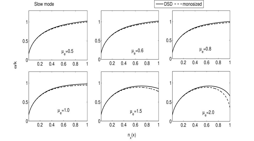
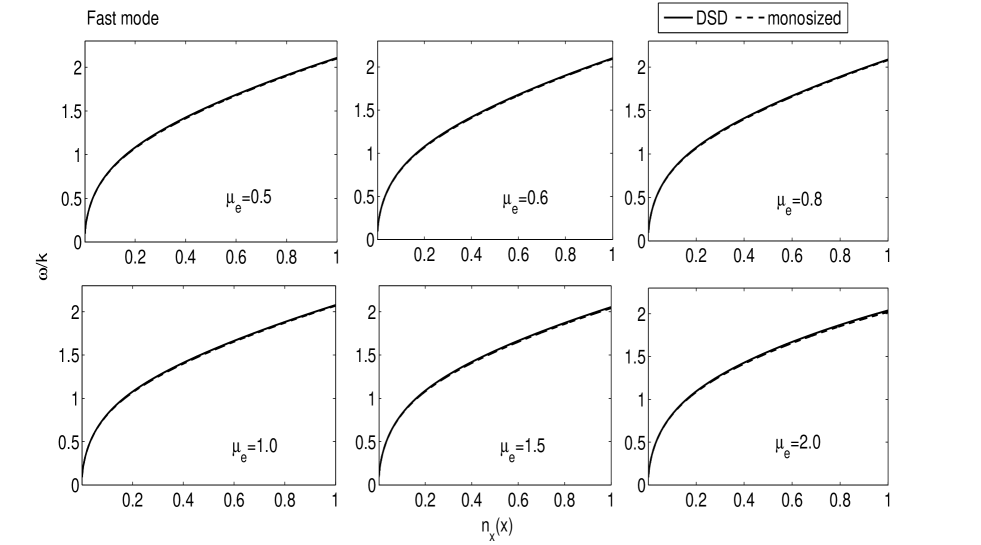
In both the cases, for slow and fast modes, it is clear from Eq. (42) that, as the wave number the phase velocity and when , . The variation of the phase velocity has been plotted with the increasing wave number for different values of in Fig.1. It shows that initially phase velocity decreases rapidly and then decreases gradually towards zero. The phase velocities are plotted against in Fig.2 for both the cases of slow and fast mode. Here, the doted lines and solid lines represent the curves for monosized and multisized dust grains, respectively. The phase velocities are plotted for the three different cases , and . In all these three cases, both in slow and fast mode, it has been noticed that due to DSD the phase velocity increases in comparison to the case of monosized dust. It is found that in fast mode, for , the phase velocity decreases along but in slow mode, for , initially the phase velocity increases and after crossing a critical value in terms of it stars decreasing gradually. However, in slow modes, as , this initial increment in phase velocities has not been observed. For , both in slow and fast mode, it has been found that above a critical value of the phase velocity becomes imaginary and so wave damping takes place. The obtained results for slow mode have been found similar to our earlier work on nonlinear waves in inhomogeneous dusty plasmasBanerjee and Maitra (2017). The curves in Fig.3 and Fig.4 represents the phase velocities for different values of in both the modes: slow and fast, respectively. The dotted and solid lines are showing the plots of phase velocities for monosized and multisized dust grains, respectively. In slow mode, as increases small increments in phase velocities have been noticed along increasing dust densities in comparison to the case of monosized dust grains. But for the case of fast mode these increments are negligibly small. It has been observed that the phase velocities increase along the increasing dust density for , but for , initially the phase velocity increases and after crossing a critical dust number density it starts decreasing, whereas in fast mode the phase velocity increases always along increasing dust density.
(a) 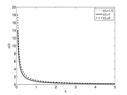 (b)
(b) 
(a) 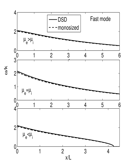 (b)
(b) 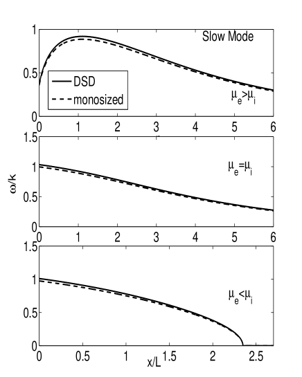
VI CONCLUSIONS
In this work, the linear analysis of dust acoustic waves have been carried out in an inhomogeneous dusty plasma having multisized negatively charged dust grains and Boltzman electrons and ions. Here, the dust grains are considered to follow power law dust size distribution. The spatial inhomogeneity in equilibrium density profiles have been considered. Assuming the spatial and time dependent perturbed quantities varies as , a dispersion relation suitable for inhomogeneous plasmas has been derived. Two different modes of wave propagation: slow and fast, have been discussed. In the case of slow mode, a critical point in terms of wave number has been derived below which wave damping occurs. Also, due to number density inhomogeneity, when the density gradient scale length of ions is large in comparison to electrons, the wave damping occurs after crossing a critical spatial distance.
Acknowledgements
One of the authors acknowledge the financially support by UGC New Delhi under the Dr. D.S. Kothari Post Doctoral Fellowship Scheme.
References
- Shukla (2001) P. K. Shukla, Physics of Plasmas 8, 1791 (2001).
- Rao et al. (1990) N. N. Rao, P. K. Shukla, and M. Y. Yu, Planetary and space science 38, 543 (1990).
- Nakamura et al. (1999) Y. Nakamura, H. Bailung, and P. K. Shukla, Physical review letters 83, 1602 (1999).
- Mendis and Rosenberg (1994) D. A. Mendis and M. Rosenberg, Annual Review of Astronomy and Astrophysics 32, 419 (1994).
- Borah et al. (2016) P. Borah, S. Bhattacharjee, and N. Das, Physics of Plasmas 23, 103706 (2016).
- Banerjee and Maitra (2016) G. Banerjee and S. Maitra, Physics of Plasmas 23, 123701 (2016).
- Losseva et al. (2012) T. V. Losseva, S. I. Popel, A. P. Golub’, Y. N. Izvekova, and P. K. Shukla, Physics of Plasmas 19, 013703 (2012).
- Shukla and Silin (1992) P. K. Shukla and V. P. Silin, Physica Scripta 45, 508 (1992).
- Singh and Rao (1998) S. V. Singh and N. N. Rao, Physics of Plasmas 5, 94 (1998).
- Liang et al. (2001) X. Liang, J. Zheng, J. X. Ma, W. D. Liu, J. Xie, G. Zhuang, and C. X. Yu, Physics of Plasmas 8, 1459 (2001).
- Hasegawa and Shukla (2004) A. Hasegawa and P. Shukla, Physics Letters A 332, 82 (2004).
- Salimullah et al. (2004) M. Salimullah, A. M. Rizwan, M. Nambu, H. Nitta, and P. Shukla, Physical Review E 70, 026404 (2004).
- Mamun et al. (1998) A. Mamun, M. Salahuddin, and M. Salimullah, Planetary and space science 47, 79 (1998).
- Mamun and Shukla (2001) A. Mamun and P. Shukla, Physics of Plasmas 8, 3513 (2001).
- Ma et al. (2012) Y.-R. Ma, C.-L. Wang, J.-R. Zhang, J.-A. Sun, W.-S. Duan, and L. Yang, Physics of Plasmas 19, 113702 (2012).
- Popel et al. (2005) S. I. Popel, T. V. Losseva, A. P. Golub, R. L. Merlino, and S. N. Andreev, Contributions to Plasma Physics 45, 461 (2005).
- Meuris (1997) P. Meuris, Planetary and space science 45, 1171 (1997).
- Duan et al. (2007) W.-S. Duan, H.-J. Yang, Y.-R. Shi, and K.-P. Lü, Physics Letters A 361, 368 (2007).
- Duan and Parkes (2003) W.-s. Duan and J. Parkes, Physical Review E 68, 067402 (2003).
- Elwakil et al. (2004) S. Elwakil, E. El-Shewy, and R. Sabry, International Journal of Nonlinear Sciences and Numerical Simulation 5, 403 (2004).
- El-Shewy et al. (2008) E. K. El-Shewy, M. A. Zahran, K. Schoepf, and S. A. Elwakil, Physica Scripta 78, 025501 (2008).
- Behery (2016) E. Behery, Physical Review E 94, 053205 (2016).
- El-Labany et al. (2013) S. K. El-Labany, W. F. El-Taibany, and E. E. Behery, Physical Review E 88, 023108 (2013).
- Behery et al. (2015) E. E. Behery, M. M. Selim, and W. F. El-Taibany, Physics of Plasmas 22, 112105 (2015).
- Maitra (2012) S. Maitra, Physics of Plasmas 19, 013701 (2012).
- Maitra and Banerjee (2014) S. Maitra and G. Banerjee, Physics of Plasmas 21, 113707 (2014).
- Banerjee and Maitra (2015) G. Banerjee and S. Maitra, Physics of Plasmas 22, 043708 (2015).
- Meuris et al. (1997) P. Meuris, F. Verheest, and G. S. Lakhina, Planetary and space science 45, 449 (1997).
- Banerjee and Maitra (2017) G. Banerjee and S. Maitra, Physics of Plasmas 24, 073702 (2017).
- Doucet et al. (1974) H. Doucet, W. Jones, and I. Alexeff, The Physics of Fluids 17, 1738 (1974).
- El-Taibany and Wadati (2007) W. F. El-Taibany and M. Wadati, Physics of plasmas 14, 042302 (2007).
- El-Taibany (2013) W. F. El-Taibany, Physics of Plasmas 20, 093701 (2013).
- Mowafy et al. (2008) A. E. Mowafy, E. K. El-Shewy, W. M. Moslem, and M. A. Zahran, Physics of Plasmas 15, 073708 (2008).
- Zadorozhny (2001) A. M. Zadorozhny, Advances in Space Research 28, 1059 (2001).