Optimal Control of Spins by Analytical Lie Algebraic Derivatives

Abstract

Computation of derivatives (gradient and Hessian) of a fidelity function is one of the most crucial steps in many optimization algorithms. Having access to accurate methods to calculate these derivatives is even more desired where the optimization process requires propagation of these calculations over many steps, which is in particular important in optimal control of spin systems. Here we propose a novel numerical approach, ESCALADE (Efficient Spin Control using Analytical Lie Algebraic Derivatives) that offers the exact first and second derivatives of the fidelity function by taking advantage of the properties of the Lie group of $2\times 2$ Hermitian matrices, $\mathrm{SU}(2)$, and its Lie algebra, the Lie algebra of skew-Hermitian matrices, $\mathfrak{su}(2)$. A full mathematical treatment of the proposed method along with some numerical examples are presented.

1 Introduction

Controlling quantum spin dynamics using time-dependent Hamiltonians in the form of pulses (e.g. radiofrequency, microwave, and laser pulses) is the essence of method development in many areas of science [1], from magnetic resonance spectroscopy and imaging [2] and terahertz technologies[3, 4] to trapped ions [5], cold atoms [6] and NV-centers in diamond [7, 8] for quantum information processing and computing [9].

In NMR and ESR, in particular, designing radiofrequency and microwave pulses for robust excitation of signals over a very wide range of frequencies and reduced sensitivity to instrumental imperfections is still among the most challenging areas of method design and is of great interest. The development of methods for pulse design in these applications generally follows one or more of three distinct routes: composite pulse design [10, 11, 12, 13, 14, 15], evolutionary numerical methods like optimal control theory (OCT) [16, 17, 2, 18, 19, 20, 21, 22], and design of swept-frequency pulses [23, 24, 25, 26, 27, 28, 29, 30, 31, 32, 33].

Two of the main challenges in the field of optimal control of spin systems are the controllability of the dynamics and the convergence rate of the control process. In principle, three main approaches can be considered when optimal control has been applied to spin systems: 1) derivative-free techniques [34, 35] which are especially important when due to experimental requirements not many iterations or function evaluations by the optimisation protocol can be allowed, 2) gradient-based techniques like GRAPE [2, 9] and KROTOV [36, 37], and 3) Newton–Raphson method [38, 39] where in addition to the gradient (first derivative), the Hessian (second derivative of the objective function with respect to the control parameters) is also utilized. Although the latter approach results in quadratic convergence rate, it suffers from numerical complexity due to computation and update of a dense Hession matrix in the course of optimization. Additionally, computation of derivatives using finite differences can be expensive, inaccurate and potentially unstable when the objective function involves numerical propagators with limited accuracy [40, Chapter 8]. Therefore having access to the exact form of these derivatives is of great interest, in particular in the optimal control of spin systems, where the optimization process requires propagation of these calculations over many steps, and inaccurate estimations of derivatives can result in a large accumulated numerical error.

The objective of this paper is to present a novel approach that facilitates the optimal control of spins using Newton–Raphson utilizing an analytical computation of derivatives. Control of dynamical systems using properties of Lie groups and their algebras covers a surprisingly wide range of applications from controlling of landing a plane, rotations of rigid bodies in robotics and estimation of camera poses in computer vision, to the time evolution of quantum systems [41, 42, 43, 44, 45, 46, 47, 48, 49]. In these applications, the underlying geometric structure is described by a Lie group. Finite difference methods suffer from a further disadvantage here since they do not respect Lie group structure and result in derivatives that do not live in the tangent space (the Lie algebra) [50].

Here we propose a novel numerical approach, ESCALADE (Efficient Spin Control using Analytical Lie Algebraic Derivatives) that harnesses the exact first and second derivatives of the fidelity function. These derivatives are computed by exploiting the properties of the Lie group of $2\times 2$ Hermitian matrices, $\mathrm{SU}(2)$, and its Lie algebra – the Lie algebra of skew-Hermitian matrices, $\mathfrak{su}(2)$. Since the Lie groups, $\mathrm{SU}(2)$ and $\mathrm{SO}(3)$ are closely related (see [51, Chapter 5] and [52, Chapter 6]), there is a close parallel between some of the properties exploited here to the Rodrigues rotation formula [53], which is utilized widely in computer vision and robotics applications for computation of rotation matrices in $\mathrm{SO}(3)$ [50, 49, 54, 55].

Although here we present the technique on the optimal control of the dynamic of non-interacting qubits, this is a general approach and can be applied to spin systems with more diverse Hamiltonian structures. It has the potential to find applications in a variety of areas where taking advantage of Lie algebra for efficient optimal control of spins is beneficial. Examples include geometric [56, 57, 41, 58, 59] and adiabatic optimal control [23, 60, 61, 62] methods.

2 Theory

2.1 Optimal control of spin-$\nicefrac{{1}}{{2}}$

The state of a single spin-$\nicefrac{{1}}{{2}}$ particle is described by the density matrix $\rho(t)\in\mathrm{SU}(2)$ and its dynamics are governed by the Liouville–von Neumann equation,

$$\partial_{t}\rho(t)=-\mathrm{i}[\mathcal{H}(t),\rho(t)],\qquad\rho(0)=\rho_{0}\in\mathrm{SU}(2),$$ (1)

where

$$\mathcal{H}(t)=\bm{h}(t)\cdot\bm{\sigma},$$ (2)

$$\bm{h}(t)=(f(t),g(t),\Omega)^{\top}\in\mathbb{R}^{3},\quad\bm{\sigma}=(\sigma_{x},\sigma_{y},\sigma_{z})^{\top},$$ (3)

and

$$\sigma_{x}=\frac{1}{2}\left(\begin{array}[]{cc}{0}&{1}\\ {1}&{0}\end{array}\right),\ \ \sigma_{y}=\frac{1}{2}\left(\begin{array}[]{cc}{0}&{-\mathrm{i}}\\ {\mathrm{i}}&{0}\end{array}\right),\ \ \sigma_{z}=\frac{1}{2}\left(\begin{array}[]{cc}{1}&{0}\\ {0}&{-1}\end{array}\right)$$

are the normalized Pauli matrices. $\Omega$ describes the offset frequency of a spin.

remark 1.

In magnetic resonance applications, it is typical to write $f(t)=\omega(t)\cos(\phi(t))$ and $g(t)=\omega(t)\sin(\phi(t))$ where the amplitude $\omega(t)$ and the phase $\phi(t)$ may be arbitrary (real-valued) functions of time.

remark 2.

In the case of multiple non-interacting spin-$\nicefrac{{1}}{{2}}$ particles, the $k$th spin evolves under the influence of $\mathcal{H}_{k}(t)=\bm{h}_{k}(t)\cdot\bm{\sigma}$, where the offset $\Omega_{k}$ in $\bm{h}_{k}(t)=(f(t),g(t),\Omega_{k})$ varies with the particle but $f(t)$ and $g(t)$ are common across all spins.

In a numerical solution of equation (1), we compute $\rho$ at time intervals $t_{0},t_{1},\ldots t_{N}$, with the unitary numerical propagation being described by

$$\rho_{n}=\mathrm{U}_{n}\rho_{n-1}\mathrm{U}_{n}^{\dagger},\qquad\mathrm{U}_{n}=\mathrm{e}^{-\mathrm{i}\bm{s}_{n}\cdot\bm{\sigma}},$$ (4)

where

$$\bm{s}_{n}=(\Delta t)\,(f(t_{n-1}),g(t_{n-1}),\Omega)^{\top}.$$ (5)

By using equation (4), one can see that the final density matrix is given by

$$\rho_{N}=\mathrm{U}_{\mathrm{tot}}\rho_{0}\mathrm{U}_{\mathrm{tot}}^{\dagger}$$ (6)

where

$$\mathrm{U}_{\mathrm{tot}}=\mathrm{U}_{N}\mathrm{U}_{N-1}\ldots\mathrm{U}_{2}\mathrm{U}_{1}.$$ (7)

Typically we want to maximize the fidelity functional,

$$\mathcal{F}=\langle\varrho|\rho_{N}\rangle:=\mathrm{Tr}(\varrho^{\dagger}\rho_{N})\quad\in[0,1],$$

to have maximum overlap (i.e. $\mathcal{F}=1$) with the (normalized) target state $\varrho\in\mathrm{SU}(2)$.

In a gradient-based optimization scheme one needs to compute the gradient of the fidelity function $\mathcal{F}$,

$$\frac{\partial\mathcal{F}}{\partial\theta_{n,k}}=\mathrm{Tr}\left(\varrho^{\dagger}\frac{\partial\rho_{N}}{\partial\theta_{n,k}}\right),$$ (8)

where $n\in\{1,\ldots,N\}$, $k\in\{1,2\}$, and

$$\theta_{n,1}=f(t_{n-1}),\qquad\theta_{n,2}=g(t_{n-1})$$

are the control parameters that solely affect the $n$th propagator, $\mathrm{U}_{n}$. A Newton–Raphson optimization scheme also requires the Hessian,

$$\frac{\partial^{2}\mathcal{F}}{\partial\theta_{m,j}\partial\theta_{n,k}}=\mathrm{Tr}\left(\varrho^{\dagger}\frac{\partial^{2}\rho_{N}}{\partial\theta_{m,j}\partial\theta_{n,k}}\right),$$ (9)

where $n,m\in\{1,\ldots,N\}$ and $j,k\in\{1,2\}$.

In the computation of the gradient of the fidelity function (8), we require the gradient of the final state $\rho_{N}$,

$$\frac{\partial\rho_{N}}{\partial\theta_{n,k}}=2\mathrm{Re}\left(\frac{\partial\mathrm{U}_{\mathrm{tot}}}{\partial\theta_{n,k}}\rho_{0}\mathrm{U}_{\mathrm{tot}}^{\dagger}\right).$$ (10)

Since $\theta_{n,k}$ only affects the $n$th propagator, this gradient can be written in the form

$$\frac{\partial\mathrm{U}_{\mathrm{tot}}}{\partial\theta_{n,k}} =\mathrm{U}_{N}\mathrm{U}_{N-1}\ldots\mathrm{U}_{n+1}\frac{\partial\mathrm{U}_{n}}{\partial\theta_{n,k}}\mathrm{U}_{n-1}\ldots\mathrm{U}_{1}$$

$$=\mathrm{L}_{n+1}\frac{\partial\mathrm{U}_{n}}{\partial\theta_{n,k}}\mathrm{R}_{n-1},$$ (11)

where

$$\mathrm{L}_{n} =\mathrm{U}_{N}\mathrm{U}_{N-1}\ldots\mathrm{U}_{n},$$ (12)

$$\mathrm{R}_{n} =\mathrm{U}_{n}\mathrm{U}_{n-1}\ldots\mathrm{U}_{1},$$ (13)

can be computed in $\mathcal{O}(N)$ time.

Here we present a method for computing the gradient $\partial\mathrm{U}_{n}/\partial\theta_{n,k}$, and therefore the gradient of the fidelity function, analytically using Lie algebraic techniques. This approach is also extended for computing the Hessian analytically.

2.2 Computation of gradient

In this section we present the analytic approach for computing the derivative of the $n$th unitary propagator (4),

$$\mathrm{U}_{n}=\exp(-\mathrm{i}\bm{s}_{n}(\theta_{n,k})),$$

with respect to a control parameter $\theta_{n,k}$. Here we write $\bm{s}_{n}(\theta_{n,k})$ to highlight the fact that $\bm{s}_{n}$ depends on $\theta_{n,k}$.

In general, the derivative of the exponential of $X(\theta)$ with respect to a control parameter $\theta$ can be expressed as [63, 64]

$$\frac{\partial}{\partial\theta}\exp(X(\theta))=\exp(X(\theta))\,\mathrm{dexp}_{X(\theta)}X^{\prime}(\theta),$$ (14)

where the dexp function,

$$\mathrm{dexp}_{X}X^{\prime}=\left(\frac{1-\mathrm{e}^{-\mathrm{ad}_{X}}}{\mathrm{ad}_{X}}\right)(X^{\prime})=\sum_{p=0}^{\infty}\frac{(-1)^{p}}{(p+1)!}\mathrm{ad}_{X}^{p}(X^{\prime}),$$ (15)

is expressed as a power series of the adjoint operator, $\mathrm{ad}$. The powers of $\mathrm{ad}$ are given by

$$\mathrm{ad}_{X}^{0}(X^{\prime}) =X^{\prime},$$

$$\mathrm{ad}_{X}(X^{\prime}) =[X,X^{\prime}],$$

$$\mathrm{ad}_{X}^{2}(X^{\prime}) =[X,[X,X^{\prime}]].$$

Equations (14) and (15) allow us to express the derivative of $\mathrm{U}_{n}$,

$$\frac{\partial\mathrm{U}_{n}}{\partial\theta_{n,k}} =\frac{\partial}{\partial\theta_{n,k}}\mathrm{e}^{-\mathrm{i}\bm{s}_{n}(\theta_{n,k})\cdot\bm{\sigma}}$$

$$=\underbrace{\mathrm{e}^{-\mathrm{i}\bm{s}_{n}\cdot\bm{\sigma}}}_{\mathrm{U}_{n}}\left(\frac{1-\mathrm{e}^{-\mathrm{ad}_{-\mathrm{i}\bm{s}_{n}\cdot\bm{\sigma}}}}{\mathrm{ad}_{-\mathrm{i}\bm{s}_{n}\cdot\bm{\sigma}}}\right)\left(-\mathrm{i}\frac{\partial\bm{s}_{n}}{\partial\theta_{n,k}}\cdot\bm{\sigma}\right)$$

$$=\mathrm{U}_{n}\left(\sum_{p=0}^{\infty}\frac{(-1)^{p}}{(p+1)!}\mathrm{ad}^{p}_{-\mathrm{i}\bm{s}_{n}\cdot\bm{\sigma}}\right)\left(-\mathrm{i}\frac{\partial\bm{s}_{n}}{\partial\theta_{n,k}}\cdot\bm{\sigma}\right).$$

remark 3.

For ease of notation, we suppress the dependence of $\bm{s}$ on the control parameters, $\theta$.

An explicit formula can be derived for the $\mathrm{dexp}$ series when $X(\theta)\in\mathrm{su}(2)$. To see this, we introduce the map $\sim$ which maps vectors in $\mathbb{R}^{3}$ to matrices in $\mathrm{su}(2)$,

$$\widetilde{\bm{s}}=-\mathrm{i}\bm{s}\cdot\bm{\sigma},\qquad\bm{s}\in\mathbb{R}^{3}.$$

It is easy to verify that

$$[\widetilde{\bm{s}},\widetilde{\bm{r}}]=\widetilde{\bm{s}\times\bm{r}}=\widetilde{\bm{S}\bm{r}},\qquad\bm{s},\bm{r}\in\mathbb{R}^{3},$$ (16)

where $\times$ is the cross product and $\bm{S}$ is the matrix,

$$\bm{S}=\left(\begin{array}[]{ccc}0&-s_{z}&s_{y}\\ s_{z}&0&-s_{x}\\ -s_{y}&s_{x}&0\\ \end{array}\right).$$ (17)

Note that the powers of the $\mathrm{ad}$ operator can be written in terms of the matrix $\bm{S}$ using the relation (16),

$$\mathrm{ad}_{-\mathrm{i}\bm{s}_{n}\cdot\bm{\sigma}}(\widetilde{\bm{r}})=\widetilde{\bm{S}_{n}\bm{r}}=-\mathrm{i}(\bm{S}_{n}\bm{r})\cdot\bm{\sigma},$$

and

$$\mathrm{ad}_{-\mathrm{i}\bm{s}_{n}\cdot\bm{\sigma}}^{p}(\widetilde{\bm{r}})=\widetilde{\bm{S}_{n}^{p}\bm{r}}=-\mathrm{i}(\bm{S}_{n}^{p}\bm{r})\cdot\bm{\sigma},\quad p\geq 0.$$

Consequently,

$$\frac{\partial\mathrm{U}_{n}}{\partial\theta_{n,k}} =-\mathrm{i}\mathrm{U}_{n}\left[\underbrace{\left(\sum_{p=0}^{\infty}\frac{(-\bm{S}_{n})^{p}}{(p+1)!}\right)}_{3\times 3}\underbrace{\left(\frac{\partial\bm{s}_{n}}{\partial\theta_{n,k}}\right)}_{{3\times 1}}\right]\cdot\bm{\sigma},$$

where $\bm{S}_{n}$ is obtained from $\bm{s}_{n}(\theta_{n,k})$ using equation (17). Observe that

$$\bm{S}_{n}^{3}=-\left\|\bm{s}_{n}\right\|^{2}\bm{S}_{n},$$

and we may further simplify the dexp series as

$$\bm{D}_{n} =\sum_{p=0}^{\infty}\frac{(-\bm{S}_{n})^{p}}{(p+1)!}$$

$$=I+\bm{S}_{n}^{2}\sum_{p=1}^{\infty}\frac{(-\left\|\bm{s}_{n}\right\|^{2})^{p-1}}{(2p+1)!}-\bm{S}_{n}\sum_{p=0}^{\infty}\frac{(-\left\|\bm{s}_{n}\right\|^{2})^{p}}{(2p+2)!}$$

$$=I+c_{1}(\left\|\bm{s}_{n}\right\|)\bm{S}_{n}+c_{2}(\left\|\bm{s}_{n}\right\|)\bm{S}_{n}^{2},$$ (18)

where

$$c_{1}(x)=\frac{\cos(x)-1}{x^{2}},\qquad c_{2}(x)=\frac{x-\sin(x)}{x^{3}}.$$ (19)

To summarise, the analytic derivative of $\mathrm{U}_{n}$ is given by

$$\frac{\partial\mathrm{U}_{n}}{\partial\theta_{n,k}}=-\mathrm{i}\mathrm{U}_{n}\left(\left[\bm{D}_{n}\frac{\partial\bm{s}_{n}}{\partial\theta_{n,k}}\right]\cdot\bm{\sigma}\right),$$ (20)

and the derivative of $\mathrm{U}_{\mathrm{tot}}$ by

$$\frac{\partial\mathrm{U}_{\mathrm{tot}}}{\partial\theta_{n,k}} =\mathrm{U}_{N}\mathrm{U}_{N-1}\ldots\mathrm{U}_{n+1}\frac{\partial\mathrm{U}_{n}}{\partial\theta_{n,k}}\mathrm{U}_{n-1}\ldots\mathrm{U}_{1}$$

$$=-\mathrm{i}\mathrm{L}_{n}\left(\left[\bm{D}_{n}\frac{\partial\bm{s}_{n}}{\partial\theta_{n,k}}\right]\cdot\bm{\sigma}\right)\mathrm{R}_{n-1}.$$ (21)

In a practical implementation, $\mathrm{L}_{n}$ and $\mathrm{L}_{n-1}$ are given by equations (12) and (13). We compute $\bm{D}_{n}$ using equation (18). Lastly, recall that in equation (5),

$$\bm{s}_{n}=(\Delta t)\,(f(t_{n-1}),g(t_{n-1}),\Omega)^{\top},$$

and the control parameters are $\theta_{n,1}=f(t_{n-1})$ and $\theta_{n,2}=g(t_{n-1})$. Consequently,

$$\frac{\partial\bm{s}_{n}}{\partial\theta_{n,1}}=(\Delta t)\,(1,0,0)^{\top},$$ (22)

and

$$\frac{\partial\bm{s}_{n}}{\partial\theta_{n,2}}=(\Delta t)\,(0,1,0)^{\top}.$$ (23)

This completes the description of the analytic gradients. Combining equations (8), (10) and (21),

$$\frac{\partial\mathcal{F}}{\partial\theta_{n,k}}=2\mathrm{Im}\mathrm{Tr}\left(\varrho^{\dagger}\mathrm{L}_{n}\left(\left[\bm{D}_{n}\frac{\partial\bm{s}_{n}}{\partial\theta_{n,k}}\right]\cdot\bm{\sigma}\right)\mathrm{R}_{n-1}\rho_{0}\mathrm{U}_{\mathrm{tot}}^{\dagger}\right).$$ (24)

Using the definition of $\mathrm{L}_{n}$ and $\mathrm{R}_{n}$ in equations (12) and (13) it is evident that $\mathrm{L}_{n}\mathrm{R}_{n-1}=\mathrm{U}_{\mathrm{tot}}$ and consequently we may write

$$\mathrm{R}_{n-1}=\mathrm{L}_{n}^{\dagger}\mathrm{U}_{\mathrm{tot}}.$$ (25)

Substituting (25) in (24) reduces the final form of the analytical gradient of the fidelity function to

$$\frac{\partial\mathcal{F}}{\partial\theta_{n,k}}=2\mathrm{Im}\mathrm{Tr}(\mathcal{L}_{n,k}\rho_{N}\varrho^{\dagger}).$$ (26)

where for any pulse segment $n$ and any control parameter $k$:

$$\mathcal{L}_{n,k}=\mathrm{L}_{n}\left(\left[\bm{D}_{n}\frac{\partial\bm{s}_{n}}{\partial\theta_{n,k}}\right]\cdot\bm{\sigma}\right)\mathrm{L}_{n}^{\dagger},$$ (27)

2.3 Computation of Hessian

In the computation of the Hessian of the fidelity function (9) we require the Hessian of the final state,

$$\frac{\partial^{2}\rho_{N}}{\partial\theta_{m,j}\partial\theta_{n,k}} =2\mathrm{Re}\left(\frac{\partial^{2}\mathrm{U}_{\mathrm{tot}}}{\partial\theta_{m,j}\partial\theta_{n,k}}\rho_{0}\mathrm{U}_{\mathrm{tot}}^{\dagger}\right.$$

$$\qquad\qquad+\left.\frac{\partial\mathrm{U}_{\mathrm{tot}}}{\partial\theta_{n,k}}\rho_{0}\frac{\partial\mathrm{U}_{\mathrm{tot}}}{\partial\theta_{m,j}}^{\dagger}\right).$$ (28)

An analytic form for the gradient of $\mathrm{U}_{\mathrm{tot}}$ with respect to control parameters $\theta_{n,k}$ and $\theta_{m,j}$ has already been obtained in equation (21). In this section, we derive an analytic form for $\partial^{2}\mathrm{U}_{\mathrm{tot}}/\partial\theta_{m,j}\partial\theta_{n,k}$.

2.3.1 Off-diagonal entries ($n>m$) of the Hessian

When $n>m$, the Hessian is typically computed as

$$\frac{\partial^{2}\mathrm{U}_{\mathrm{tot}}}{\partial\theta_{m,j}\partial\theta_{n,k}} =\underbrace{\mathrm{U}_{N}\mathrm{U}_{N-1}\ldots\mathrm{U}_{n+1}}_{\mathrm{L}_{n+1}}\frac{\partial\mathrm{U}_{n}}{\partial\theta_{n,k}}$$

$$\qquad\times\underbrace{\mathrm{U}_{n-1}\ldots\mathrm{U}_{m+1}}_{\mathrm{M}_{n-1,m+1}}\frac{\partial\mathrm{U}_{m}}{\partial\theta_{m,j}}$$

$$\qquad\quad\times\underbrace{\mathrm{U}_{m-1}\ldots\mathrm{U}_{1}}_{\mathrm{R}_{m-1}}.$$ (29)

where

$$\mathrm{M}_{n,m} =\mathrm{U}_{n}\mathrm{U}_{n-1}\ldots\mathrm{U}_{m-1}\mathrm{U}_{m}.$$ (30)

Similarly, we can derive the corresponding expression for $m>n$. Overall, since $n$ and $m$ range between $1$ and $N$, the various values of $\mathrm{M}_{n,m}$ are typically computed in $\mathcal{O}(N^{2})$ time in such a procedure.

Here we introduce an alternative approach for computing $\partial^{2}\mathrm{U}_{\mathrm{tot}}/\partial\theta_{m,j}\partial\theta_{n,k}$ that does not require the computation of $\mathrm{M}_{n,m}$. Since $\mathrm{L}_{n+1}$ and $\mathrm{R}_{m-1}$ are unitary,

$$\mathrm{L}_{n+1}^{\dagger}\mathrm{L}_{n+1}=I,\qquad\mathrm{R}_{m-1}^{\dagger}\mathrm{R}_{m-1}=I,$$ (31)

we can express $\mathrm{M}_{n,m}$ as

$$\mathrm{M}_{n,m} =\mathrm{U}_{n}\mathrm{U}_{n-1}\ldots\mathrm{U}_{m}$$

$$=\mathrm{L}_{n+1}^{\dagger}\mathrm{L}_{n+1}\mathrm{U}_{n}\mathrm{U}_{n-1}\ldots\mathrm{U}_{m}\mathrm{R}_{m-1}\mathrm{R}_{m-1}^{\dagger}$$

$$=\mathrm{L}_{n+1}^{\dagger}\mathrm{U}_{\mathrm{tot}}\mathrm{R}_{m-1}^{\dagger}.$$ (32)

Thus, $\mathrm{M}_{n,m}$ can be replaced in the computation of the Hessian and equation (29) can be written in the form

$$\frac{\partial^{2}\mathrm{U}_{\mathrm{tot}}}{\partial\theta_{m,j}\partial\theta_{n,k}}=\mathrm{L}_{n+1}\frac{\partial\mathrm{U}_{n}}{\partial\theta_{n,k}}\mathrm{L}_{n}^{\dagger}\mathrm{U}_{\mathrm{tot}}\mathrm{R}_{m}^{\dagger}\frac{\partial\mathrm{U}_{m}}{\partial\theta_{m,j}}\mathrm{R}_{m-1}.$$ (33)

Substituting (20), the expression in equation (33) becomes

$$-\mathrm{L}_{n+1}\mathrm{U}_{n}\left(\left[\bm{D}_{n}\frac{\partial\bm{s}_{n}}{\partial\theta_{n,k}}\right]\cdot\bm{\sigma}\right)\mathrm{L}_{n}^{\dagger}\mathrm{U}_{\mathrm{tot}}$$

$$\qquad\qquad\quad\times\mathrm{R}_{m}^{\dagger}\mathrm{U}_{m}\left(\left[\bm{D}_{m}\frac{\partial\bm{s}_{m}}{\partial\theta_{m,j}}\right]\cdot\bm{\sigma}\right)\mathrm{R}_{m-1}.$$

We use the fact that $\mathrm{L}_{n+1}\mathrm{U}_{n}=\mathrm{L}_{n}$ and $\mathrm{R}_{m}^{\dagger}\mathrm{U}_{m}=\mathrm{R}_{m-1}^{\dagger}$ to reduce this expression to

$$-\mathrm{L}_{n}\left(\left[\bm{D}_{n}\frac{\partial\bm{s}_{n}}{\partial\theta_{n,k}}\right]\cdot\bm{\sigma}\right)\mathrm{L}_{n}^{\dagger}\mathrm{U}_{\mathrm{tot}}$$

$$\qquad\qquad\quad\times\mathrm{R}_{m-1}^{\dagger}\left(\left[\bm{D}_{m}\frac{\partial\bm{s}_{m}}{\partial\theta_{m,j}}\right]\cdot\bm{\sigma}\right)\mathrm{R}_{m-1}.$$

2.3.2 Diagonal entries ($m=n$) of the Hessian

For the case $m=n$, following (11),

$$\frac{\partial^{2}\mathrm{U}_{\mathrm{tot}}}{\partial\theta_{n,j}\partial\theta_{n,k}}=\mathrm{L}_{n+1}\frac{\partial^{2}\mathrm{U}_{n}}{\partial\theta_{n,j}\partial\theta_{n,k}}\mathrm{R}_{n-1}.$$ (34)

Differentiating equation (20) with respect to $\theta_{n,j}$,

$$\frac{\partial^{2}\mathrm{U}_{n}}{\partial\theta_{n,j}\partial\theta_{n,k}}=$$

$$\qquad-\mathrm{U}_{n}\left\{\left[\left(\bm{D}_{n}\frac{\partial\bm{s}_{n}}{\partial\theta_{n,j}}\right)\cdot\bm{\sigma}\right]\left[\left(\bm{D}_{n}\frac{\partial\bm{s}_{n}}{\partial\theta_{n,k}}\right)\cdot\bm{\sigma}\right]\right.$$

$$\qquad\left.+\mathrm{i}\left(\frac{\partial\bm{D}_{n}}{\partial\theta_{n,j}}\frac{\partial\bm{s}_{n}}{\partial\theta_{n,k}}+\bm{D}_{n}\frac{\partial^{2}\bm{s}_{n}}{\partial\theta_{n,j}\partial\theta_{n,k}}\right)\cdot\bm{\sigma}\right\},$$ (35)

where $\partial^{2}\bm{s}_{n}/\partial\theta_{n,j}\partial\theta_{n,k}$ vanishes due to (22) and (23). The derivative of $\bm{D}_{n}$ (18) can be computed explicitly,

$$\frac{\partial\bm{D}_{n}}{\partial\theta_{n,j}} =\frac{\partial}{\partial\theta_{n,j}}\left(I+c_{1}(\left\|\bm{s}_{n}\right\|)\bm{S}_{n}+c_{2}(\left\|\bm{s}_{n}\right\|)\bm{S}_{n}^{2}\right)$$ (36)

$$=c_{1}^{\prime}(\left\|\bm{s}_{n}\right\|)\frac{\partial\left\|\bm{s}_{n}\right\|}{\partial\theta_{n,j}}\bm{S}_{n}+c_{1}(\left\|\bm{s}_{n}\right\|)\frac{\partial\bm{S}_{n}}{\partial\theta_{n,j}}$$

$$\qquad+c_{2}^{\prime}(\left\|\bm{s}_{n}\right\|)\frac{\partial\left\|\bm{s}_{n}\right\|}{\partial\theta_{n,j}}\bm{S}_{n}^{2}$$

$$\qquad+c_{2}(\left\|\bm{s}_{n}\right\|)(\bm{S}_{n}\frac{\partial\bm{S}_{n}}{\partial\theta_{n,j}}+\frac{\partial\bm{S}_{n}}{\partial\theta_{n,j}}\bm{S}_{n}),$$

where

$$c_{1}^{\prime}(x) =\frac{-2\cos(x)-x\sin(x)+2}{x^{3}},$$ (37)

$$c_{2}^{\prime}(x) =\frac{3\sin(x)-x\cos(x)-2x}{x^{4}},$$ (38)

$$\frac{\partial\left\|\bm{s}_{n}\right\|}{\partial\theta_{n,j}}=\frac{\bm{s}_{n}\cdot\frac{\partial\bm{s}_{n}}{\partial\theta_{n,j}}}{\left\|\bm{s}_{n}\right\|},$$ (39)

and $\partial\bm{S}_{n}/\partial\theta_{n,j}$ is obtained directly by creating a matrix from $\partial\bm{s}_{n}/\partial\theta_{n,j}$, equations (22) and (23), along the lines of (17),

$$\frac{\partial\bm{S}_{n}}{\partial\theta_{n,1}}=(\Delta t)\left(\begin{array}[]{ccc}0&0&0\\ 0&0&-1\\ 0&1&0\\ \end{array}\right),\ \frac{\partial\bm{S}_{n}}{\partial\theta_{n,2}}=(\Delta t)\left(\begin{array}[]{ccc}0&0&1\\ 0&0&0\\ -1&0&0\\ \end{array}\right).$$ (40)

The complete description of the Hessian of the fidelity is obtained by combining equations (9), (28), (29), (35), (34) and (21),

$$\frac{\partial^{2}\mathcal{F}}{\partial\theta_{m,j}\partial\theta_{n,k}}=2\mathrm{Re}\mathrm{Tr}(\varrho^{\dagger}(\mathcal{V}_{m,n,j,k}-\mathcal{W}_{m,n,j,k})),$$ (41)

where

$$\mathcal{V}_{m,n,j,k} =\mathrm{L}_{n}\left(\left[\bm{D}_{n}\frac{\partial\bm{s}_{n}}{\partial\theta_{n,k}}\right]\cdot\bm{\sigma}\right)\mathrm{R}_{n-1}\rho_{0}$$

$$\qquad\times{\left(\mathrm{L}_{m}\left(\left[\bm{D}_{m}\frac{\partial\bm{s}_{m}}{\partial\theta_{m,j}}\right]\cdot\bm{\sigma}\right)\mathrm{R}_{m-1}\right)}^{\dagger},$$ (42)

Using equations (25) and (27) we can simplify the above expressions as follows:

$$\mathcal{V}_{m,n,j,k}=\mathcal{L}_{n,k}\rho_{N}\mathcal{L}_{m,j}^{\dagger}$$ (43)

while $\mathcal{V}_{m,n,j,k}$ is common between diagonal ($m=n$) and off-diagonal elements ($n>m$) of the Hessian matrix $\mathcal{W}_{m,n,j,k}$ has two distinct forms.
For $m=n$,

$$\mathcal{W}_{n,n,j,k} =\mathrm{L}_{n}\left\{\left[\left(\bm{D}_{n}\frac{\partial\bm{s}_{n}}{\partial\theta_{n,j}}\right)\cdot\bm{\sigma}\right]\left[\left(\bm{D}_{n}\frac{\partial\bm{s}_{n}}{\partial\theta_{n,k}}\right)\cdot\bm{\sigma}\right]\right.$$

$$\qquad\quad\left.+\mathrm{i}\left[\left(\frac{\partial\bm{D}_{n}}{\partial\theta_{n,j}}\frac{\partial\bm{s}_{n}}{\partial\theta_{n,k}}\right)\cdot\bm{\sigma}\right]\right\}\mathrm{R}_{n-1}\rho_{0}\mathrm{U}_{\mathrm{tot}}^{\dagger},$$

and for $n>m$,

$$\mathcal{W}_{m,n,j,k} =\mathrm{L}_{n}\left(\left[\bm{D}_{n}\frac{\partial\bm{s}_{n}}{\partial\theta_{n,k}}\right]\cdot\bm{\sigma}\right)\mathrm{L}_{n}^{\dagger}\mathrm{U}_{\mathrm{tot}}$$

$$\qquad\times\mathrm{R}_{m-1}^{\dagger}\left(\left[\bm{D}_{m}\frac{\partial\bm{s}_{m}}{\partial\theta_{m,j}}\right]\cdot\bm{\sigma}\right)\mathrm{R}_{m-1}\rho_{0}\mathrm{U}_{\mathrm{tot}}^{\dagger}.$$

Similar to equation (43) we can do additional simplifications for the $\mathcal{W}_{m,n,j,k}$ term. For $m=n$ we have:

$$\mathcal{W}_{n,n,j,k}=\left(\mathcal{L}_{n,j}\mathcal{L}_{n,k}+\mathcal{D}_{n,j,k}\right)\rho_{N}$$ (44)

where

$$\mathcal{D}_{n,j,k}=\mathrm{i}\mathrm{L}_{n}\left[\left(\frac{\partial\bm{D}_{n}}{\partial\theta_{n,j}}\frac{\partial\bm{s}_{n}}{\partial\theta_{n,k}}\right)\cdot\bm{\sigma}\right]\mathrm{L}_{n}^{\dagger}.$$ (45)

and for $n>m$ we can use equation (27) to write:

$$\mathcal{W}_{m,n,j,k}=\mathcal{L}_{n,k}\mathcal{L}_{m,j}\rho_{N}$$ (46)

Therefore the general form of the diagonal elements of the Hessian matrix will be:

$$\frac{\partial^{2}\mathcal{F}}{\partial\theta_{n,j}\partial\theta_{n,k}} =2\mathrm{Re}\mathrm{Tr}(\mathcal{L}_{n,k}\rho_{N}\mathcal{L}_{n,j}^{\dagger}\varrho^{\dagger}$$

$$\qquad\qquad-(\mathcal{L}_{n,j}\mathcal{L}_{n,k}+\mathcal{D}_{n,j,k})\rho_{N}\varrho^{\dagger}),$$ (47)

and the general form of the upper-diagonal elements of the Hessian matrix can be written as

$$\frac{\partial^{2}\mathcal{F}}{\partial\theta_{m,j}\partial\theta_{n,k}}=2\mathrm{Re}\mathrm{Tr}(\mathcal{L}_{n,k}\rho_{N}\mathcal{L}_{m,j}^{\dagger}\varrho^{\dagger}-\mathcal{L}_{n,k}\mathcal{L}_{m,j}\rho_{N}\varrho^{\dagger}),$$ (48)

$\mathcal{L}$ and $\mathcal{D}$ can be precomputed in $\mathcal{O}(N)$ time along with $\mathrm{L}$. The factorization (27) reduces the computational effort by a factor of three since only two matrix multiplications are required for each entry of the Hessian. Note that the lower-diagonal elements ($n<m$) can be easily obtained using the symmetry of the Hessian matrix and do not need to be computed separately. Equation (48) for these entries can be written as:

$$\frac{\partial^{2}\mathcal{F}}{\partial\theta_{m,j}\partial\theta_{n,k}}=2\mathrm{Re}\mathrm{Tr}(\mathcal{L}_{n,k}\rho_{N}\mathcal{L}_{m,j}^{\dagger}\varrho^{\dagger}-\mathcal{L}_{m,j}\mathcal{L}_{n,k}\rho_{N}\varrho^{\dagger}),$$ (49)

Finally, using equations (47), (48) and (49) a general form of Hessian entries can be expressed as a single equation:

$$\frac{\partial^{2}\mathcal{F}}{\partial\theta_{m,j}\partial\theta_{n,k}} =2\mathrm{Re}\mathrm{Tr}(\mathcal{L}_{n,k}\rho_{N}\mathcal{L}_{m,j}^{\dagger}\varrho^{\dagger}$$

$$\qquad-(\underbrace{\mathcal{L}_{n,k}\mathcal{L}_{m,j}}_{\underset{\text{if }m>n}{\mathcal{L}_{m,j}\mathcal{L}_{n,k}}}+\underbrace{\mathcal{D}_{n,j,k}}_{\underset{\text{if }n\neq m}{0}})\rho_{N}\varrho^{\dagger}),$$ (50)

3 Numerical demonstrations

3.1 Comparison with finite difference method

Finite difference approximation of the gradient of numerical propagators $U_{n}$ requires computing $U_{n}$ for multiple values of $\theta_{n,k}$ differing by a ‘finite difference step’. Figure 1 demonstrates that while the finite difference step size must be kept sufficiently small for accuracy, the approximations become unstable for very small steps. Thus the suitability of a finite difference step may prove difficult to asses a-priori. This balance between accuracy and stability becomes more precarious when (i) the time step of the numerical propagator ($\Delta t$) is large, (ii) the numerical propagator is of limited accuracy or (iii) higher derivatives are required. In addition to respecting the Lie algebraic structure and being relatively inexpensive, the proposed approach for computing analytic derivatives does not suffer from such instability.

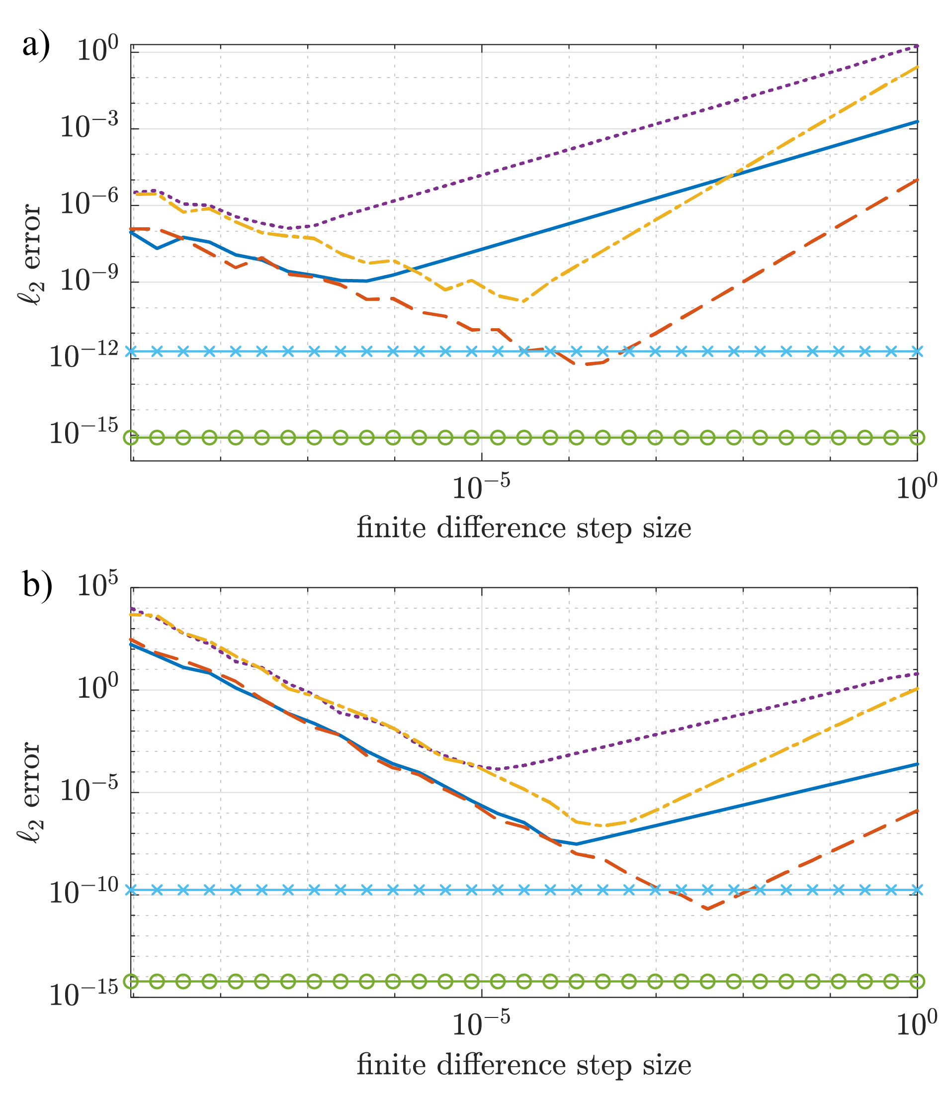
Figure 1: Accuracy and stability of forward differences and central differences approximation to (a) the gradient ($\partial U_{n}/\partial\theta_{n,k}$), and (b) the Hessian ($\partial^{2}U_{n}/\partial\theta_{n,k}^{2}$) of a single step propagator $U_{n}$. The behaviour is shown for two different time steps, $\Delta t=10^{-6}$ (forward difference [solid blue], central difference [dotted purple], analytic [solid green with circles]) and $\Delta t=10^{-4}$ (forward difference [dashed orange], central difference [densely dashed yellow], analytic [solid light blue with crosses]).

3.2 Example for pulse design in magnetic resonance

Here we demonstrate one of the applications of the proposed method for the design of broadband excitation pulses in magnetic resonance spectroscopy. The simplest case would be control of an ensemble of non-interacting spin-$\nicefrac{{1}}{{2}}$ particles. Conventional instantaneous radio-frequency or microwave pulses have limited bandwidth due to high power requirements that cannot be afforded on most instruments; therefore they can only satisfy the desired state manipulation in a rather limited range of frequencies close to the transmitter offset of the pulse, i.e. they are only effective for spins with relatively small frequency offsets; additionally, the performance of these pulses can be considerably affected by instrumental imperfections or instabilities. The goal here is to circumvent these problems by designing a pulse propagator that satisfies certain objectives for all spins within the desired frequency range, with a robust performance that does not depend on frequency offset of spins or instrumental imperfections.

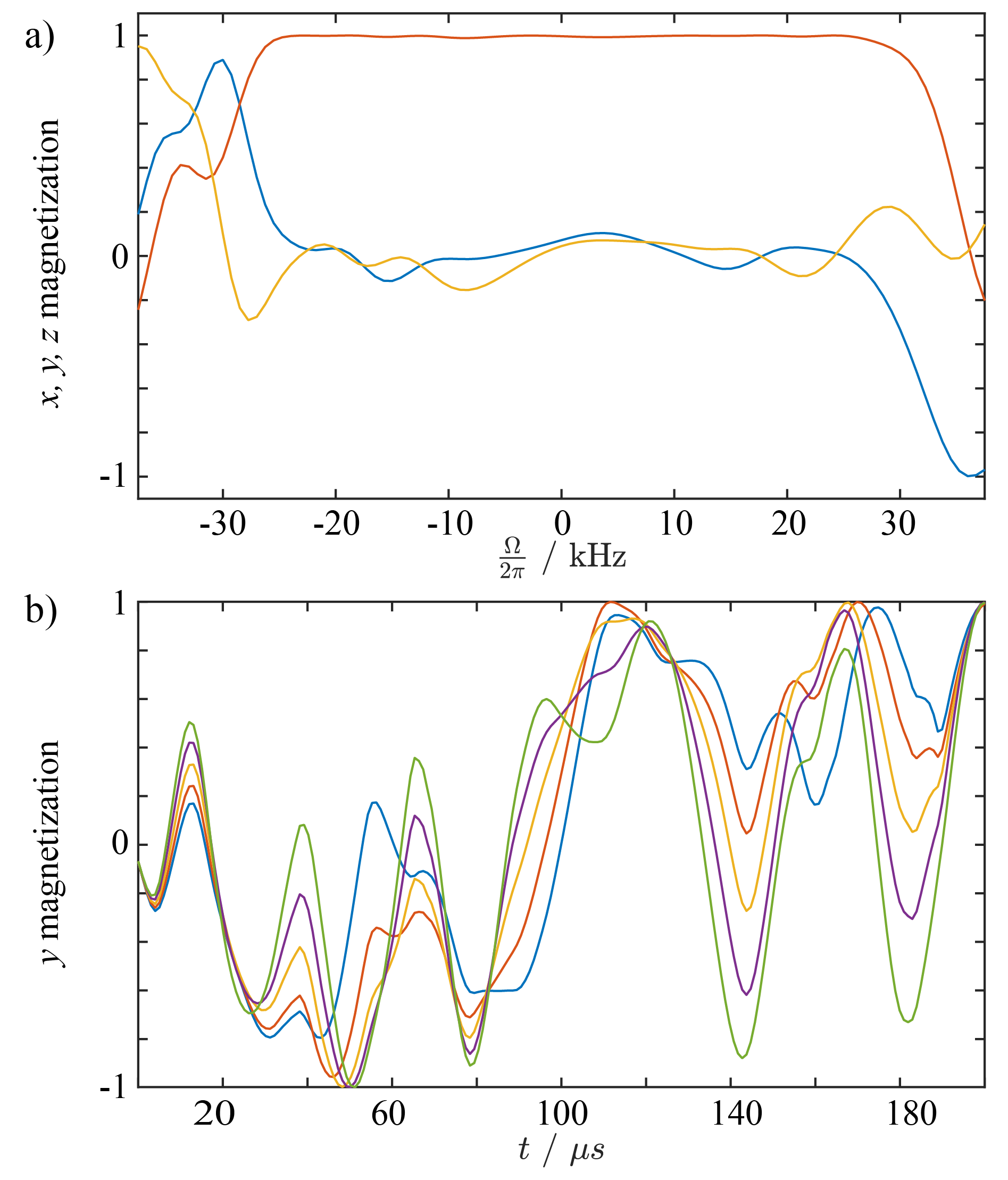
Figure 2: (a) calculated excitation profiles for different component of density operator, $x$ (blue), $y$ (red), and $z$ (orange) at $\omega_{1}=\omega_{1}^{0}$ (20 kHz) for a 200 $\mu$s pulse acting on 101 non-interacting spin-$\nicefrac{{1}}{{2}}$ over a 50 kHz frequency range; (b) variations of $y$ component of spin trajectories during the pulse for five different frequencies.

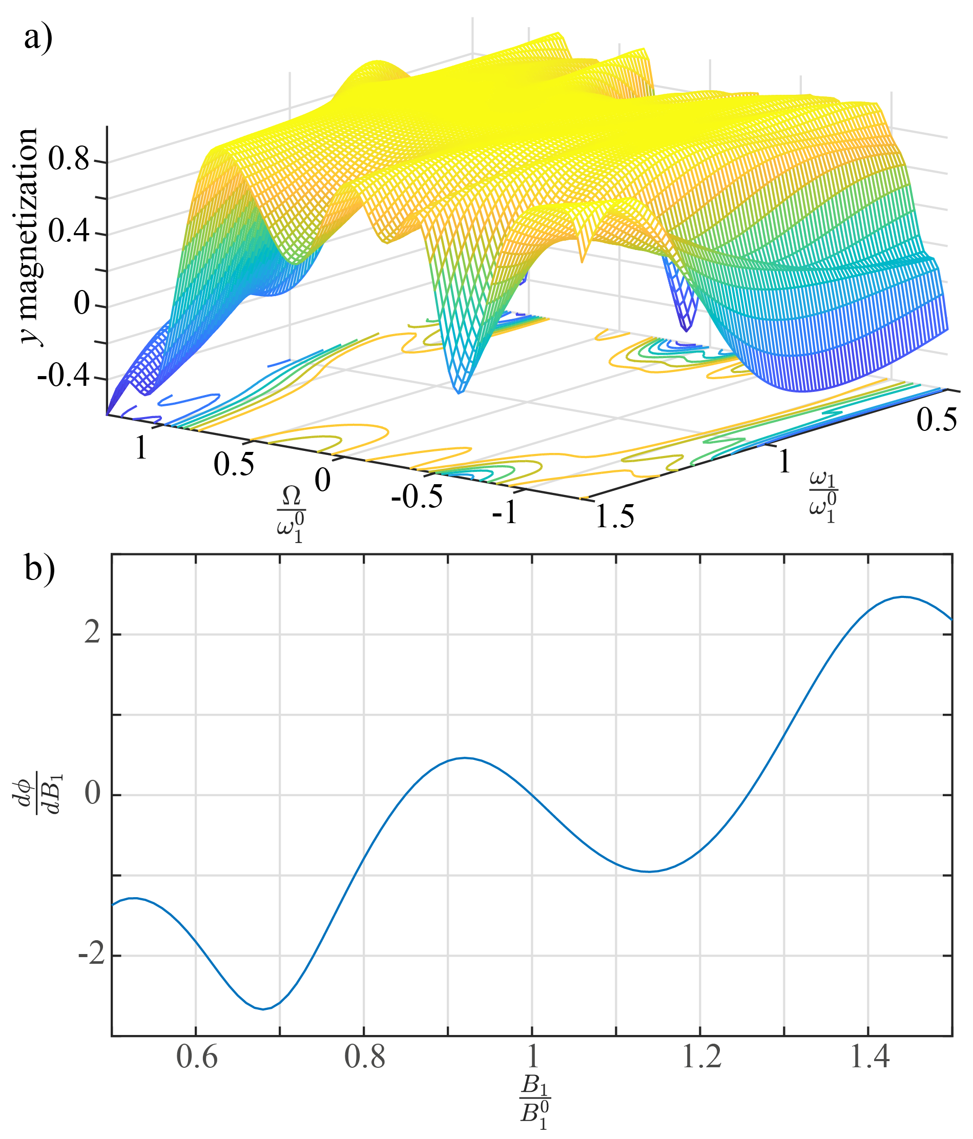
Figure 3: (a) 3D plot and projection showing the $y$-magnetization excited as a function of relative resonance offset ($\frac{\Omega}{\omega_{1}^{0}}$) and relative RF amplitude $\frac{\omega_{1}}{\omega_{1}^{0}}$; (b) Sensitivity of signal phase to field strength ($\frac{\mathrm{d}\phi}{\mathrm{d}B_{1}}$) as a function of relative field strength ($\frac{B_{1}}{B_{1}^{0}}$).

The example here demonstrates an excitation pulse designed using the proposed method to bring all spins in the ensemble from $z$ to $y$. Figure 2 (a) shows the final state of spin across the frequency range of interest (50 kHz here), and figure 2 (a) shows variations of one of the components, $y$, for five different offset frequencies during the 200 $\mu$s pulse. Additionally, we can incorporate an additional optimization step that significantly reduces the sensitivity of the pulse to instrumental imperfections. Here this was considered as reducing the sensitivity of the pulse performance to unknown variations of radio-frequency (RF), or microwave (MW) amplitudes. Figure 3 (a) shows corresponding graphs for the variations of the target state, $y$, versus RF field, $B_{1}$. One common example of such imperfection is the position-dependent $B_{1}$ field across an RF coil used to generate the pulse. These variations introduce position-dependent phase of the signal across the ensemble of spins and therefore results in significant signal loss and non-uniform excitation profile of the pulse. Here an additional objective is to minimize the variation of signal phase with respect to the variation of $B_{1}$ field ($\frac{\mathrm{d}\phi}{\mathrm{d}B_{1}}$), figure 3 (b) shows that for a given nominal RF amplitude with $\pm 20\%$ variations in the amplitude of $B_{1}$ field, $\frac{\mathrm{d}\phi}{\mathrm{d}B_{1}}$ is zero for all frequencies in the desired range.

4 Conclusion

In the present work, we have introduced a new approach, ESCALADE, for computation of derivatives of the cost function in optimal control of spin systems. We demonstrated that using the proposed mathematical framework, derivatives (gradient and Hessian) can be computed analytically using Lie algebraic techniques. The proposed method is very general and can be adapted to and used in many potential applications where efficient optimal control of spin systems is required. A numerical implementation of the proposed method in MATLAB along with additional functions for optimization and visualization of the performance are freely available via the following DOI: 10.17632/8zz84359m5.1.

References

- [1] S. J. Glaser, U. Boscain, T. Calarco, C. P. Koch, W. Köckenberger, R. Kosloff, I. Kuprov, B. Luy, S. Schirmer, T. Schulte-Herbrüggen, D. Sugny, F. K. Wilhelm, Training schrödinger’s cat: quantum optimal control, Eur. Phys. J. D 69 (12) (2015).
- [2] N. Khaneja, T. Reiss, C. Kehlet, T. Schulte-Herbruggen, S. J. Glaser, Optimal control of coupled spin dynamics: design of nmr pulse sequences by gradient ascent algorithms, J. Magn. Reson. 172 (2) (2005) 296–305.
- [3] E. Rasanen, A. Castro, J. Werschnik, A. Rubio, E. K. Gross, Optimal control of quantum rings by terahertz laser pulses, Phys. Rev. Lett. 98 (15) (2007) 157404.
- [4] L. H. Coudert, Optimal control of the orientation and alignment of an asymmetric-top molecule with terahertz and laser pulses, J. Chem. Phys. 148 (9) (2018).
- [5] M. Zhao, D. Babikov, Coherent and optimal control of adiabatic motion of ions in a trap, Phys. Rev. A 77 (1) (2008).
- [6] J. C. Saywell, I. Kuprov, D. L. Goodwin, M. Carey, T. Freegarde, Optimal control of mirror pulses for cold-atom interferometry, Phys. Rev. A 98 (2) (2018).
- [7] Y. Chou, S. Huang, H. Goan, Optimal control of fast and high-fidelity quantum gates with electron and nuclear spins of a nitrogen-vacancy center in diamond, Phys. Rev. A 91 (5) (2015).
- [8] J. Tian, T. Du, Y. Liu, H. Liu, F. Jin, R. S. Said, J. Cai, Optimal quantum optical control of spin in diamond, Phys. Rev. A 100 (1) (2019).
- [9] D. Lu, K. Li, J. Li, H. Katiyar, A. J. Park, G. Feng, T. Xin, H. Li, G. Long, A. Brodutch, J. Baugh, B. Zeng, R. Laflamme, Enhancing quantum control by bootstrapping a quantum processor of 12 qubits, Npj Quantum Inf. 3 (1) (2017) 45.
- [10] M. H. Levitt, R. R. Ernst, Composite pulses constructed by a recursive expansion procedure, J. Magn. Reson. 55 (2) (1983) 247–254.
- [11] A. J. Shaka, R. Freeman, Composite pulses with dual compensation, J. Magn. Reson. 55 (3) (1983) 487–493.
- [12] M. H. Levitt, D. Suter, R. R. Ernst, Composite pulse excitation in three-level systems, J. Chem. Phys. 80 (7) (1984) 3064–3068.
- [13] R. Tycko, H. M. Cho, E. Schneider, A. Pines, Composite pulses without phase distortion, J. Magn. Reson. 61 (1) (1985) 90–101.
- [14] M. H. Levitt, Composite pulses, Prog. NMR Spectrosc. 18 (2) (1986) 61–122.
- [15] A. J. Shaka, A. Pines, Symmetric phase-alternating composite pulses, J. Magn. Reson. 71 (3) (1987) 495–503.
- [16] N. Khaneja, R. Brockett, S. J. Glaser, Time optimal control in spin systems, Phys. Rev. A 63 (3) (2001) 1–13.
- [17] N. Khaneja, T. Reiss, B. Luy, S. J. Glaser, Optimal control of spin dynamics in the presence of relaxation, J. Magn. Reson. 162 (2) (2003) 311–319.
- [18] K. Kobzar, B. Luy, N. Khaneja, S. J. Glaser, Pattern pulses: design of arbitrary excitation profiles as a function of pulse amplitude and offset, J. Magn. Reson. 173 (2) (2005) 229–35.
- [19] Z. Tosner, T. Vosegaard, C. Kehlet, N. Khaneja, S. J. Glaser, N. C. Nielsen, Optimal control in nmr spectroscopy: numerical implementation in simpson, J. Magn. Reson. 197 (2) (2009) 120–34.
- [20] K. Kobzar, S. Ehni, T. E. Skinner, S. J. Glaser, B. Luy, Exploring the limits of broadband 90 degrees and 180 degrees universal rotation pulses, J. Magn. Reson. 225 (2012) 142–60.
- [21] I. Kuprov, Spin system trajectory analysis under optimal control pulses, J. Magn. Reson. 233 (2013) 107–12.
- [22] E. Van Reeth, H. Rafiney, M. Tesch, S. J. Glaser, D. Sugny, Optimizing mri contrast with b1 pulses using optimal control theory, in: Proc. IEEE Int. Symp. Biomed. Imaging, 2016, pp. 310–313.
- [23] T. Kato, On the adiabatic theorem of quantum mechanics, J. Phys. Soc. Jpn. 5 (6) (1950) 435–439.
- [24] J. Baum, R. Tycko, A. Pines, Broadband population inversion by phase modulated pulses, J. Chem. Phys. 79 (9) (1983) 4643–4644.
- [25] J. Baum, R. Tycko, A. Pines, Broadband and adiabatic inversion of a two-level system by phase-modulated pulses, Phys. Rev. A 32 (6) (1985) 3435–3447.
- [26] D. Kunz, Use of frequency-modulated radiofrequency pulses in mr imaging experiments, Magn. Reson. Med. 3 (3) (1986) 377–84.
- [27] T. Fujiwara, K. Nagayama, Optimized frequency/phase-modulated broadband inversion pulses, J. Magn. Reson. 86 (3) (1990) 584–592.
- [28] R. Fu, G. Bodenhausen, Broadband decoupling in nmr with frequency-modulated ‘chirp’ pulses, Chem. Phys. Lett. 245 (4-5) (1995) 415–420.
- [29] Ē. Kupče, R. Freeman, Adiabatic pulses for wideband inversion and broadband decoupling, J. Magn. Reson. A 115 (2) (1995) 273–276.
- [30] A. Doll, G. Jeschke, Fourier-transform electron spin resonance with bandwidth-compensated chirp pulses, J. Magn. Reson. 246 (2014) 18–26.
- [31] J. E. Power, M. Foroozandeh, R. W. Adams, M. Nilsson, S. R. Coombes, A. R. Phillips, G. A. Morris, Increasing the quantitative bandwidth of nmr measurements, Chem. Commun. 52 (14) (2016) 2916–9.
- [32] N. Khaneja, Chirp excitation, J. Magn. Reson. 282 (2017) 32–36.
- [33] M. Foroozandeh, M. Nilsson, G. A. Morris, Improved ultra-broadband chirp excitation, J. Magn. Reson. 302 (2019) 28–33.
- [34] C. Cartis, J. Fiala, B. Marteau, L. Roberts, Improving the flexibility and robustness of model-based derivative-free optimization solvers, ACM Trans. Math. Softw. 45 (3) (2019) 1–41.
- [35] D. L. Goodwin, W. K. Myers, C. R. Timmel, I. Kuprov, Feedback control optimisation of esr experiments, J. Magn. Reson. 297 (2018) 9–16.
- [36] R. Eitan, M. Mundt, D. J. Tannor, Optimal control with accelerated convergence: Combining the krotov and quasi-newton methods, Phys. Rev. A 83 (5) (2011).
- [37] S. G. Schirmer, P. de Fouquieres, Efficient algorithms for optimal control of quantum dynamics: the krotov method unencumbered, New J. Phys. 13 (7) (2011).
- [38] P. de Fouquieres, S. G. Schirmer, S. J. Glaser, I. Kuprov, Second order gradient ascent pulse engineering, J. Magn. Reson. 212 (2) (2011) 412–7.
- [39] D. L. Goodwin, I. Kuprov, Modified newton-raphson grape methods for optimal control of spin systems, J. Chem. Phys. 144 (20) (2016) 204107.
- [40] J. Nocedal, S. J. Wright, Numerical Optimization, 2nd Edition, Springer, New York, NY, USA, 2006.
- [41] V. Jurdjevic, Optimal control on lie groups and integrable hamiltonian systems, Regul. Chaotic Dyn. 16 (5) (2011) 514–535.
- [42] G. C. Walsh, R. Montgomery, S. S. Sastry, Optimal path planning on matrix lie groups, in: Proc. IEEE Conf. Decis. Control, Vol. 2, 1994, pp. 1258–1263.
- [43] S. Amari, Natural gradient works efficiently in learning, Neural Comput. 10 (2) (1998) 251–276.
- [44] Y. Nishimori, Learning algorithm for independent component analysis by geodesic flows on orthogonal group, in: Proc. Int. Jt. Conf. Neural Netw., Vol. 2, 1999, pp. 933–938.
- [45] M. D. Plumbley, Lie group methods for optimization with orthogonality constraints, in: C. G. Puntonet, A. Prieto (Eds.), Independent Component Analysis and Blind Signal Separation, Springer Berlin Heidelberg, Berlin, Heidelberg, 2004, pp. 1245–1252.
- [46] G. Dirr, U. Helmke, K. Hüper, M. Kleinsteuber, Y. Liu, Spin dynamics: A paradigm for time optimal control on compact lie groups, J. Global Optim. 35 (3) (2006) 443–474.
- [47] K. Spindler, Optimal control on lie groups: Theory and applications, WSEAS Trans. Math. 12 (5) (2013) 531–542.
- [48] T. Drummond, R. Cipolla, Application of lie algebras to visual servoing, Int. J. Comput. Vis. 37 (1) (2000) 21–41.
- [49] O. Tuzel, R. Subbarao, P. Meer, Simultaneous multiple 3d motion estimation via mode finding on lie groups, in: Tenth IEEE International Conference on Computer Vision (ICCV’05) Volume 1, Vol. 1, 2005, pp. 18–25 Vol. 1.
- [50] C. J. Taylor, D. J. Kriegman, Minimization on the lie group so(3) and related manifolds, Tech. Rep. 9405, Yale University (1994).
- [51] Y. Kosmann-Schwarzbach, Groups and Symmetries, Springer, 2010. doi:10.1007/978-0-387-78866-1.
- [52] P. Woit, Quantum Theory, Groups and Representations, Springer, 2017. doi:10.1007/978-3-319-64612-1.
- [53] Rodrigues, Des lois géométriques qui régissent les déplacements d’un système solide dans l’espace, et de la variation des coordonnées provenant de ces déplacements considérés indépendamment des causes qui peuvent les produire., J. Math. Pures Appl. (1840) 380–440.
- [54] G. Gallego, A. Yezzi, A compact formula for the derivative of a 3-d rotation in exponential coordinates., J. Math. Imaging Vis. 51 (2015) 378–384.
- [55] G. Terzakis, M. Lourakis, D. Ait-Boudaoud, Modified rodrigues parameters: An efficient representation of orientation in 3d vision and graphics, J. Math. Imaging Vis. 60 (3) (2018) 422–442.
- [56] N. Khaneja, S. J. Glaser, R. Brockett, Sub-riemannian geometry and time optimal control of three spin systems: Quantum gates and coherence transfer, Phys. Rev. A 65 (3) (2002) 1–11.
- [57] N. Khaneja, S. Glaser, R. Brockett, Subriemannian geodesics and optimal control of spin systems, Proc. Am. Control Conf. 4 (2002) 2806–2811.
- [58] B. Bonnard, S. J. Glaser, D. Sugny, A review of geometric optimal control for quantum systems in nuclear magnetic resonance, Adv. Math. Phys. 2012 (2012) 1–29.
- [59] B. Bonnard, O. Cots, S. J. Glaser, M. Lapert, D. Sugny, Z. Yun, Geometric optimal control of the contrast imaging problem in nuclear magnetic resonance, IEEE Trans. Autom. Control 57 (8) (2012) 1957–1969.
- [60] C. Brif, M. D. Grace, M. Sarovar, K. C. Young, Exploring adiabatic quantum trajectories via optimal control, New J. Phys. 16 (6) (2014) 065013.
- [61] S. Meister, J. T. Stockburger, R. Schmidt, J. Ankerhold, Optimal control theory with arbitrary superpositions of waveforms, J. Phys. A 47 (49) (2014).
- [62] N. Augier, U. Boscain, M. Sigalotti, Adiabatic ensemble control of a continuum of quantum systems, SIAM J. Control Optim. 56 (6) (2018) 4045–4068.
- [63] F. Schur, Zur theorie der endlichen transformationsgruppen, Abh. Math. Sem. Univ. Hamburg 4 (1891) 15–32.
- [64] W. Rossmann, Lie Groups: An Introduction Through Linear Groups, Oxford University Press, 2006.