Flow Computation in Temporal Interaction Networks

Abstract

Temporal interaction networks capture the history of activities between entities along a timeline. At each interaction, some quantity of data (money, information, kbytes, etc.) flows from one vertex of the network to another. Flow-based analysis can reveal important information. For instance, financial intelligent units (FIUs) are interested in finding subgraphs in transactions networks with significant flow of money transfers. In this paper, we introduce the flow computation problem in an interaction network or a subgraph thereof. We propose and study two models of flow computation, one based on a greedy flow transfer assumption and one that finds the maximum possible flow. We show that the greedy flow computation problem can be easily solved by a single scan of the interactions in time order. For the harder maximum flow problem, we propose graph precomputation and simplification approaches that can greatly reduce its complexity in practice. As an application of flow computation, we formulate and solve the problem of flow pattern search, where, given a graph pattern, the objective is to find its instances and their flows in a large interaction network. We evaluate our algorithms using real datasets. The results show that the techniques proposed in this paper can greatly reduce the cost of flow computation and pattern enumeration.

1 Introduction

Temporal interaction networks model the transfer of data quantities between entities along a timeline. At each interaction, a quantity (money, messages, kbytes etc.) flows from one network vertex (entity) to another. Analyzing interaction networks can reveal important information (e.g., cyclic transactions, message interception). For instance, financial intelligent units (FIUs) are often interested in finding subgraphs of a transaction network, wherein vertices (financial entities) have exchanged a significant amount of money directly or through intermediaries (e.g., multiple small-volume transactions through a subnetwork that aggregate to large amounts). Such exchanges may be linked to criminal behavior (e.g., money laundering). In addition, significant money flow in the bitcoin transaction network has been associated to theft [23].

Problem. In this paper, we study the problem of computing the flow through an interaction network (or a sub-network thereof), from a designated vertex $s$, called source to a designated vertex $t$, called sink. As an example, Figure 1(a) shows a toy interaction network, where vertices are bank accounts and each edge is a sequence of interactions in the form $(t_{i},q_{i})$, where $t_{i}$ is a timestamp and $q_{i}$ is the transferred quantity (money). To model and solve the flow computation problem from $s$ to $t$, we assume that throughout the history of interactions, each vertex $v$ has a buffer $B_{v}$. Since we are interested in measuring the flow from $s$ to $t$, we assume that initially $s$ has infinite buffer and that the buffers of all other vertices are $0$. Interactions are examined in order of time and, as a result of an interaction $(t_{i},q_{i})$ on edge $(v,u)$, vertex $v$ may transfer from $B_{v}$ to $u$’s buffer $B_{u}$ a quantity in $[0,q_{i}]$. For example, if interaction $(1,\$3)$ on edge $(s,x)$ transfers $\$3$ from $B_{s}$ to $B_{x}$, interaction $(5,\$5)$ on edge $(x,z)$ can transfer at most $\$3$ from $B_{x}$ to $B_{z}$. After the end of the timeline, the buffered quantity at the sink vertex $t$ models the flow that has been transferred from $s$ to $t$.

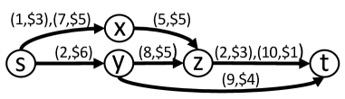
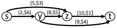
(a) interaction network	(b) simplified network

Figure 1: A toy interaction network

We study two models of flow transfer as an effect of an interaction $(t_{i},q_{i})$ on an edge $(v,u)$. The first one is based on a greedy flow transfer assumption, where $v$ transfers to $u$ the maximum possible quantity, i.e., $\min\{q_{i},B_{v}\}$. According to the second model, $v$ may transfer to $u$ any quantity in $[0,\min\{q_{i},B_{v}\}]$, reserving the remaining quantity for future outgoing interactions from $v$ (to any vertex). The objective is then to compute the maximum flow that can be transferred from $s$ to $t$. In our running example, as a result of interaction $(2,\$6)$ on edge $(s,y)$, $\$6$ are transferred from $B_{s}$ to $B_{y}$. As a result of interaction $(8,\$5)$ on edge $(y,z)$, the greedy model transfers $\$5$ (i.e., the maximum possible amount) from $B_{y}$ to $B_{z}$, leaving only $\$1$ to $B_{y}$ for future interactions. Hence, interaction $(9,\$4)$ on edge $(y,t)$ may only transfer $\$1$ to the buffer $B_{t}$ of the sink. Had interaction $(8,\$5)$ transferred only $\$2$ from $B_{y}$ to $B_{z}$, interaction $(9,\$4)$ would be able to transfer $\$4$ from $B_{y}$ to $B_{t}$. This decision would maximize the flow that reaches $t$.

Applications. Flow computation in interaction networks finds application in different domains. As already discussed, computing the flow of money from one financial entity (e.g., back customer, cryptocurrency user) to another can help in defining their relationship and the roles of any intermediaries in them [16]. As another application, consider a transportation network (e.g., flights network, road network) and the problem of computing the maximum flow (e.g., of vehicles or passengers) from a source to a destination. Identifying cases of heavy flow transfer can help in improving the scheduling or redesigning the network. Similarly, in a communications network, measuring the flow between vertices (e.g., routers) can help in identifying abnormalities (e.g., attacks) or bad design. Recent studies in cognitive science [4] associate the information flow in the human brain with the embedded network topology and the interactions between different (possibly distant) regions.

Contributions. We show that the greedy flow computation problem can be solved very fast by performing only a linear scan of all interactions in order of time and updating two buffers at each interaction. However, greedy flow computation is of less interest and has fewer applications compared to the more challenging maximum flow computation problem. The latter is not always solved by greedy flow computation, as we have shown with the example of Figure 1(a). We show how the maximum flow problem can be formulated and solved using linear programming (LP). In a nutshell, we can define one variable for each interaction (except from those originating from the source vertex $s$, which always transfer the maximum possible flow) and find the values of the variables that maximize the total flow that ends up at the sink.

Flow computation in networks is not a new problem, however, previous work has mainly focused on the classic maximum flow problem in a static graph, where vertices are junctions and edges have capacities [6]. Our problem setup is quite different, since our vertices model entities and edges are time-series of interactions, each of which happens at a specific timestamp. However, as we show, our problem turns out to be equivalent to a temporal flow computation problem, where the edges (and their capacities) are ephemeral. Akrida et al. [2] show that this temporal flow computation problem is equivalent to flow computation in a static graph, where an edge is defined for each ephemeral edge, meaning that the complexity of our problem is quadratic to the number of interactions (e.g., if Edmonds–Karp algorithm [7] is used).

Hence, solving the maximum flow problem on a network with numerous interactions can be quite expensive. We propose a set of techniques that reduce the cost in practice. First, we show that for certain classes of networks (such as simple paths), the greedy algorithm can compute (exactly) the maximum flow in linear time to the number of interactions. Verifying whether greedy can compute the maximum flow costs only a single pass over the vertices. Second, we propose a preprocessing algorithm that eliminates interactions, edges and vertices that cannot contribute to the maximum flow, with a potential to greatly reduce the problem size and complexity. For example, interaction $(2,\$3)$ on edge $(z,t)$ of the network in Figure 1(a) can be eliminated because all incoming interactions to $z$ have timestamps greater than $2$; hence, interaction $(2,\$3)$ cannot transfer any incoming quantity to $z$. Third, we design an algorithm that performs greedy flow computation on a part of the graph, simplifying the graph on which LP has to be eventually applied. For example, the path formed by edges $(s,x)$ and $(x,z)$ can be reduced to a single edge $(s,z)$ as shown in Figure 1(b), because not propagating the maximum possible flow through this path to $z$ and reserving flow at $s$ or $x$ cannot increase the maximum flow that eventually reaches $t$. We conduct an experimental evaluation, where we compute the flow on subgraphs of three large real networks and show that our maximum flow computation approach is very effective, achieving at least one order of magnitude cost reduction compared to the baseline LP algorithm.

As an application of flow computation, we also formulate and study the problem of flow pattern search in large interaction networks. These patterns as small graphs that repeat themselves in the network. The problem is to find the instances and compute the flow for each of them. We propose a graph preprocessing approach that facilitates the enumeration of certain classes of patterns and their maximum flows. As we show experimentally, enumerating the instances of flow patterns and computing their flow can greatly benefit from the precomputed data.

The contributions of this paper can be summarized as follows:

• This is the first work, to our knowledge, which studies flow computation in temporal interaction networks. We propose two models for flow computation and analyze their complexities. The first model comes together with a greedy computation algorithm, while maximum flow computation can be formulated and solved as a linear programming problem.

• For maximum flow computation, which can be expensive, we propose (i) an efficient check for verifying if it can be solved exactly by the greedy algorithm, (ii) a graph preprocessing technique, which can eliminate interactions, vertices and edges from the graph, (iii) a graph simplification approach, which reduces part of the graph to edges, the flow of which can be derived using the greedy algorithm.

• We formulate and study a flow pattern enumeration problem which computes instances of graph patterns in a large graph and their flows. We show that a graph preprocessing technique can accelerate pattern enumeration.

• We conduct experiments using data from three real interaction networks to evaluate our techniques.

Outline. The rest of the paper is organized as follows. Section 2 reviews work related to flow computation on static and temporal graphs and to pattern enumeration on large networks. Section 3 defines basic concepts and Section 4 defines flow computation models and algorithms. In Section 5, we study the problem of flow pattern search. A thorough experimental evaluation on real data is presented in Section 6. Finally, Section 7 concludes the paper with directions for future work.

2 Related Work

There have been numerous studies that investigate the problems of flow computation in networks and enumeration of patterns in graphs. In this section, we summarize the most representative works for the above problems and discuss their relation to our study.

2.1 Flow Computation

Ford and Fulkerson [8] were the first who tracked the max-flow problem. Given a DAG, with a source node $s$ with no incoming edges and a sink node $t$ with no outgoing edges and assuming that each edge has a capacity, the Ford-Fulkerson algorithm finds the maximum flow that can be transferred from $s$ to $t$ through the edges of the network, assuming that each edge has a maximum capacity for flow transfer. The algorithm applies on static networks, in which the existence of edges and their capacities do not change over time. In addition, the flow is assumed to be transferred instantly from one vertex to another and to be constant over time. Since then, a number of models and algorithms for maximum flow computation have been developed [1, 11].

Skutella [31] surveyed temporal maximum flow computation problems. In these problems, each edge, besides having a capacity, is characterized by a transit time, i.e., the time needed to transfer flow equal to its capacity [15]. The general problem is to find the maximum flow that can be transferred from $s$ to $t$ within a time horizon $T$ [3, 29]. In another model for temporal flow computation, each edge is assumed to be ephemeral, i.e., it cannot be used to transfer flow at any time. Akrida et al. [2] studied the max-flow problem in such networks. They assume that each edge is valid at certain days (e.g., day 5 and day 8). Similar to [31], the problem is to find the maximum flow that can be transferred from $s$ to $t$ by the end of day $l$. The capacity of an edge is the amount of flow that it can transfer each day that it is valid. The vertices of the network have a buffer, meaning that they can hold a maximum amount of flow before this can be transferred by an outgoing edge that will become available in the future. Flow computation when the capacities of the edges are time-varying was also studied in [13].

As opposed to all temporal flow computation problems studied in previous work [31, 2] we do not consider networks where edges have capacities (variable or constant), but edges having sequences of instantaneous interactions with flow, which take place at specific timestamps. Our objective is to compute the flow from a given source to a given sink vertex considering all interactions on the edges. Still, as we show in Section 4.2.1, the maximum flow version of our problem is equivalent to the problem formulated and studied in [2], if we consider the interactions as ephemeral capacities of the edges. Besides showing this equivalence, in Section 4.2, we propose novel graph preprocessing and simplification techniques that greatly reduce the worst-case cost of maximum flow computation in practice.

Flow computation in temporal networks is also related to similar problems, but with a quite different formulation and goal. For instance, Kumar et al. [19] study the identification of interaction sequences between nodes forming paths in the network, which model potential pathways for information spread.

2.2 Network Patterns

A number of works in the literature study the enumeration of graph patterns in static and temporal networks. One of the earliest works is on motifs search [24]. Motifs are small patterns that repeat themselves in a network much more frequently than expected. Paranjape et al. [26] define motifs in temporal networks [14], by extending the definition of [24], to consider the temporal information of the interactions between the graph vertices. Specifically, such motifs are small connected graphs whose edges are temporally ordered. An instance of a motif is a sequence of interactions which have the structure of the motif and respect the time order of the motif’s edges. In addition, the time difference between the first and the last interaction in the instance should not exceed a maximum threshold. The objective of motif search is to count the instances of one or more motifs in a large network.

Kosyfaki et al. [18] defined and studied the enumeration of flow motifs in interaction networks, considering both the time and the flow on the interactions. Such motifs come with two constraints: the maximum possible duration a motif instance and the minimum possible flow of the motif. Although we also study the enumeration of flow patterns in Section 5, (i) our flow computation model is very different compared to the one in [18], as we consider maximum flow computation and also allow time-interleaving sequences of interactions, (ii) we study patterns that are not limited to simple paths, (iii) we propose precomputation approaches for pattern enumeration.

Pattern matching and enumeration in general graphs and temporal networks is a well-studied problem [9, 30, 32, 27, 28, 33]. Sun et al. study the problem of pattern matching in large networks [32]. They propose STwig, an algorithm that combines graph exploration and joining intermediate results. Moreover, their algorithm can adapted to work in parallel. An older work [5] formulates and solves the pattern matching problem by joining the edges of the graph in a systematic way. The enumeration of cyclic patterns in a temporal network was recently studied in [20]. Züfle et al. [34] study the temporal relations between entities in social networks. For this purpose, they enumerate temporal patterns with the help of a data structure that indexes small pattern instances. Mining frequent patterns in static and temporal networks has also been studied in previous work [12, 21, 22].

For graphs, where vertices (and/or edges) of the graph and the patterns are labeled, pattern matching is relatively easy, as vertex labels (or small subgraphs) can be indexed and search/join algorithms can be used to accelerate search. The flow pattern search problem that we study in Section 5 is more challenging, because there are no constraints as to which vertices of the graph can match the vertices of a pattern. In addition, there is no previous work on enumerating pattern instances and their maximum flows, i.e., the problem that we study in Section 5.

3 Definitions

In this section, we define basic concepts and summarize the most frequently used notation. We begin by formally defining an interaction network.

Definition 1 (Interaction Network)

An interaction network is a directed graph $G(V,E)$. For each edge $e=(v,u)$ of the network, there is a sequence $e_{S}=\{(t_{1},q_{1}),(t_{2},q_{2}),\dots\}$ of interactions from node $v$ to node $u$. Each interaction $(t_{i},q_{i})$ has a quantity $q_{i}$, which is transferred from $v$ to $u$ at timestamp $t_{i}$.

Figure 2(a) shows an example of a network, where edges are annotated with the corresponding sequences of interactions.

In practice, an data analyst would be interested in measuring the total flow from a specific source vertex of the network to a specific sink vertex of the network. The source and the sink might coincide. In addition, the analyst might only want to include certain vertices and edges in the subgraph for which the flow is to be measured.

One way to select interesting subgraphs on which the flow should be measured is by specifying a network pattern, i.e., the structure that the interesting subgraphs should conform to, and identify their instances in the interaction network. We now provide definitions for a network pattern and its instances.

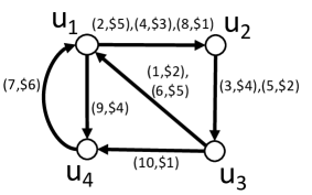
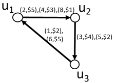
(a) interaction network	(b) pattern	(c) instance

Figure 2: Network, pattern, and instance

Definition 2 (Network Pattern)

A network pattern $G_{P}(V_{P},E_{P})$ is a directed acyclic graph, where each vertex $v\in V_{P}$ has a label $\ell(v)$.

Definition 3 (Instance)

An instance of pattern $G_{P}$ in graph $G$ is a subgraph $G_{M}(V_{M},E_{M})$ of $G_{T}$, such that

• there is a surjection $\mu:V_{P}\to V_{M}$ from the vertex set $V_{P}$ of the pattern $G_{P}$ to the vertex set $V_{M}$ of $G_{M}$;

• for two vertices $v,u$ of $G_{P}$, $\mu(v)=\mu(u)$ iff $\ell(v)=\ell(u)$;

• $(v,u)\in E_{P}$ iff $(\mu(v),\mu(u))\in E_{M}$.

We assume that the network $G$, in which we search for pattern instances is not labeled. The labels on the vertices of a pattern are only used to indicate that pattern vertices having the same labels should be mapped to the same graph vertex in a pattern instance. Continuing the example of Figure 2, consider the network pattern $G_{P}$ shown in Figure 2(b) which includes 4 nodes connected in a chain. Since the first and the last vertex of $G_{P}$ have the same label, this pattern corresponds to a cyclic transaction (i.e., $a$ transfers some quantity to $b$, then $b$ transfers to $c$, then $c$ transfers to $a$). Figure 2(c) shows an instance of this pattern, which is a subgraph of the interaction network that satisfies Definition 3 (i.e., $a$ is mapped to $u_{1}$, $b$ to $u_{2}$, and $c$ to $u_{3}$).

In the next section, we define and study the problem of computing the total quantity that flows throughout an interaction network or a subgraph thereof, from a given source to a given sink vertex, before studying the problem of enumerating network patterns and their flows in Section 5. Table 1 summarizes the notation used frequently in the paper.

Table 1: Table of notations

Notations	Description
$G(V,E)$	input graph
$(t_{i},q_{i})$	an interaction with quantity $q_{i}$ at time $t_{i}$
$src_{i}$ ($dest_{i}$)	source (destination) vertex of interaction $(t_{i},q_{i})$
$e_{S}=\{(t_{1},q_{1}),(t_{2},q_{2}),\dots\}$	sequence of interactions on edge $e$
$B_{v}$	total quantity buffered at node $v$
$B^{t_{i}}_{v}$	buffer at node $v$ by time $t_{i}$
$G_{P}(V_{P},E_{P})$	network pattern
$G_{M}(V_{M},E_{M})$	instance a network pattern
$\mu(v)$	vertex of $V_{M}$ mapped to vertex $v\in V_{P}$

4 Flow Computation

Here, we focus on the problem of flow computation from a given source to a given sink vertex, in an interaction (sub-)network. Figure 3 illustrates an example of such a network, consisting of four vertices and five edges. Each edge has a sequence $\{(t_{i},q_{i})\}$ of interactions; in this example, each sequence has only one interaction.

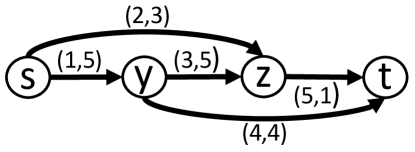
Figure 3: Example of a graph

We consider two definitions of the flow computation problem and how they relate to each other. First, in greedy flow computation, we take interactions in order of time and assume that every interaction $(t_{i},q_{i})$ greedily transfers the maximum possible quantity to the target vertex, given the quantity accumulated until time $t_{i}$ to the source vertex of the interaction. For example, in the graph of Figure 3, interaction $(t_{i},q_{i})=(3,5)$ on edge $(y,z)$ transfers a quantity of $q_{i}=5$ from $y$ to $z$, because $y$ has received $5$ due to interaction $(t_{j},q_{j})=(1,5)$ on edge $(s,y)$ which happened before ($t_{j}<t_{i}$). On the other hand, in maximum flow computation, we consider the case where a vertex may reserve some quantity for future interactions, if that could maximize the maximum overall flow that can be transferred throughout the DAG. For example, in Figure 3, interaction $(t_{i},q_{i})=(3,5)$ on edge $(y,z)$ may transfer any quantity in $[0,5]$, since vertex $y$ has accumulated $5$ units, by time $3$. Both definitions comply to the principle that a interaction $(t_{i},q_{i})$ on an edge $(v,u)$ cannot transfer a larger quantity than what the source vertex $v$ has received from its incoming interactions before time $t_{i}$ and was not yet transferred via its outgoing interactions before time $t_{i}$.

In both definitions of flow computation, we consider connected graphs which have just one source node (with no incoming edges) and just one sink node with no outgoing edges (like the graph of Figure 3). Our methods and algorithms can easily be extended for graphs with multiple sources. In this case, we can add a synthetic source vertex $s$ and an edge from $s$ to each original source. Similarly, if there are multiple sinks, we can add a synthetic sink vertex $t$ and an edge from each original sink to the synthetic one. Each of the outgoing edges from the synthetic source are given a single interaction with the smallest possible timestamp and an infinite quantity (in order for the original sources to be able to transfer any quantity via their outgoing edges). Each of the incoming edges of the synthetic sink are given a single interaction with the largest possible timestamp and an infinite quantity (in order for the original sinks to be able to absorb any quantity via their incoming edges; these are eventually accumulated at the synthetic sink). Figure 4 shows an example of a graph before and after adding the source and the sink. In the rest of the paper, we assume that each input graph to our flow computation problem is connected and has a single source vertex $s$ with no incoming edges and a single sink vertex $t$ with no outgoing edges. The objective is to compute the flow from $s$ to $t$.

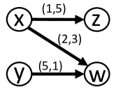
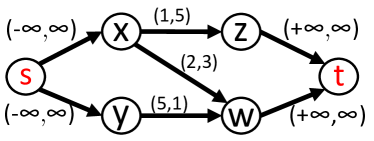
(a) Example of a DAG	(b) Additional source and sink

Figure 4: Example of synthetic source and sink addition

4.1 Greedy flow computation

In this section, we define and solve the greedy flow computation problem in a graph $G$. To compute the flow $f(G)$ throughout $G$, we assume that each vertex $v\in G$ keeps, in a buffer $B_{v}$, the total quantity received from its incoming interactions. We denote by $B^{t_{i}}_{v}$ the value of the buffer by time $t_{i}$. The source vertex $s$ of $G$ is assumed to constantly have infinite quantity in its buffer, i.e., $B^{t_{i}}_{s}=\infty,\forall t$. This means that for each interaction $(t_{i},q_{i})$ that comes out of $s$, the entire quantity $q_{i}$ is transferred to the buffer of the destination vertex. Before the temporally first interaction in $G$, the buffers of all nodes (except for the source) are $0$. The flow computation process considers all interactions at the edges of $E$ in order of time. Each interaction, say from vertex $v$ to vertex $u$ greedily transfers the maximum possible quantity from $B_{v}$ to $B_{u}$. We do not set a bound on how much a node can buffer and buffered quantities do not expire. Formally, flow computation is based on the following definition of greedy flow transfer.

Definition 4 (Greedy Flow Transfer)

As an effect of interaction $(t_{i},q_{i})$ on edge $(v,u)\in G$, $v$ transfers to $u$ at time $t_{i}$, a quantity $q=\min\{q_{i},B^{t_{i}}_{v}\}$, where $B^{t_{i}}_{v}$ is the total quantity buffered in $v$ by time $t_{i}$. As a result of the flow transfer, $B^{t_{i}}_{v}$ is reduced by $q$ and $B^{t_{i}}_{u}$ is increased by $q$.

In simple words, as a result of a interaction, a node transfers as much as possible from its buffered quantity via the interaction. After the last interaction in $G$, the total quantity buffered at the sink vertex of $G$ is the flow $f(G)$. Formally,

Definition 5 (Greedy flow of graph $G$)

The flow $f(G)$ of a graph $G$ is the total quantity buffered at the sink of $G$ after processing all interactions in $G$ in temporal order and applying for each interaction Definition 4 to update the buffered quantities of nodes.

Table 2 shows the steps of computing $f(G)$ of the graph shown in 3. Since $s$ is the source node of the graph, $B_{s}$ is always $\infty$. In addition, $t$ is the sink, hence, $f(G)$ will be equal to $B_{t}$, after processing all interactions. The first column shows the currently examined interaction, the second column the edge where it belongs and the last four columns the changes in the buffers of the vertices after the interaction is processed. In the beginning, $B_{s}=\infty$ and the buffers of all other vertices are $0$. The temporally first interaction $(1,5)$ on edge $(s,y)$ transfers $5$ units from $B_{s}$ to $B_{y}$. Then, $(2,3)$ on edge $(s,z)$ transfers $3$ units from $B_{s}$ to $B_{z}$. Then, $(3,5)$ on edge $(y,z)$ transfers $\min\{B_{y},5\}=5$ units from $B_{y}$ to $B_{z}$, which results in $B_{y}=0$ and $B_{z}=8$. Interaction $(4,4)$ on edge $(y,t)$ transfers no units, as $\min\{B_{y},4\}=0$. Finally, interaction $(5,1)$ on edge $(z,t)$ transfers $\min\{B_{z},1\}=1$ units from $B_{z}$ to $B_{t}$ and the total flow of the DAG is considered to be $B_{t}=1$.

Table 2: Example of greedy flow computation

$(t_{i},q_{i})$	$(v,u)$	$B_{s}$	$B_{y}$	$B_{z}$	$B_{t}$
$(1,5)$	$(s,y)$	$\infty$	$5$	$0$	$0$
$(2,3)$	$(s,z)$	$\infty$	$5$	$3$	$0$
$(3,5)$	$(y,z)$	$\infty$	$0$	$8$	$0$
$(4,4)$	$(y,t)$	$\infty$	$0$	$8$	$0$
$(5,1)$	$(z,t)$	$\infty$	$0$	$7$	$1$

Complexity analysis. It is easy to show that the flow $f(G)$ of a graph $G$ can be computed in time linear to the number of interactions on the edges of $G$, assuming that these can be accessed in order of time. This is due to the fact that each interaction causes the update of at most two vertex buffers, hence, processing an interaction takes constant time.

4.2 Maximum Flow computation

The flow transfer definition of the previous section (Definition 4) does not consider the case where, as a result of an interaction on edge $(v,u)$, $v$ does not transfer the maximum possible quantity to $u$, but reserves quantity for future interactions. As a result, the quantity $f(G)$ computed by Definition 5 might not be the maximum possible. To illustrate this, consider again the graph of Figure 3. As shown in Table 2, due to interaction $(3,5)$, vertex $y$ transfers all its buffered quantity (i.e., $5$) to $z$, hence $B_{y}$ becomes 0 and $B_{z}$ becomes 8. As a result, at the temporally next interaction $(4,4)$, which is on edge $(y,t)$, $y$ cannot transfer any quantity to $t$ because $B_{y}=0$ at that time. Had $y$ transferred to $z$ a quantity of $1$ unit (instead of $5$) at the interaction $(3,5)$, $y$ would have saved $4$ units in its buffer to use at interaction $(4,4)$. This change maximizes the total flow that is transferred throughout the graph, as shown in Table 3. In general, the flow computed by the greedy algorithm can be arbitrarily smaller than the maximum possible flow.

Table 3: Example of maximum flow computation

$(t_{i},q_{i})$	$(v,u)$	$B_{s}$	$B_{y}$	$B_{z}$	$B_{t}$
$(1,5)$	$(s,y)$	$\infty$	$5$	$0$	$0$
$(2,3)$	$(s,z)$	$\infty$	$5$	$3$	$0$
$(3,5)$	$(y,z)$	$\infty$	$4$	$4$	$0$
$(4,4)$	$(y,t)$	$\infty$	$0$	$4$	$4$
$(5,1)$	$(z,t)$	$\infty$	$0$	$3$	$5$

Hence, assuming that vertices can transfer any portion of their reserved quantity at an interaction, an interesting problem is finding the maximum flow that can be transferred from the source to the sink of the graph $G$. In this section, we analyze this problem and show that it is equivalent to a maximum flow computation problem in temporal graphs [2], which can be solved by linear programming (LP). We show that for specific classes of graphs $G$ (e.g., chains), greedy flow computation gives us the solution to the maximum flow problem. In addition, to reduce the cost of maximum flow computation, we propose a preprocessing approach, which eliminates interactions (and possibly edges and vertices of the graph) which are guaranteed do not affect the solution. Finally, we present a graph simplification approach, which computes part of the solution using the greedy algorithm and, consequently, reduce the overall cost maximum flow computation.

4.2.1 Formulation as an LP problem and equivalence to a known problem

We first formulate the maximum flow computation problem as a linear programming (LP) problem. The problem includes one variable $x_{i}$ for each interaction $(t_{i},q_{i})$ at any edge. Variable $x_{i}$ corresponds to the quantity that will be transferred as a result of the interaction. Since the transferred quantity cannot be negative and cannot exceed $q_{i}$, we have:

$$0\leq x_{i}\leq q_{i}$$ (1)

For the special case, where the interaction originates from the source vertex, we have $x_{i}=q_{i}$, since we assume that the source has infinite buffer (i.e., reducing the units transferred from the source vertex cannot increase the total quantity that reaches the sink). Hence, the number of variables can be reduced to the number of interactions that do not originate from the source. In addition, we have the constraint that an interaction $(t_{i},q_{i})$ on edge $(src_{i},dest_{i})$ cannot transfer more than the total incoming units to $src_{i}$ minus the total outgoing units from $src_{i}$, up to timestamp $t_{i}$:

$$x_{i}\leq\sum_{dest_{j}=src_{i}\land t_{j}<t_{i}}x_{j}-\sum_{src_{j}=src_{i}\land t_{j}<t_{i}}x_{j}$$ (2)

The objective of the LP problem is to find the values of all variables $x_{i}$, which will maximize the quantity that will arrive at the sink vertex. Hence, the objective is:

$$\textrm{maximize~{}}\sum_{dest_{i}=sink(G)}{x_{i}}$$ (3)

We will now show that our problem is equivalent to the maximum flow computation problem in temporal graphs, studied in [2]. Specifically, a temporal flow network, as defined in [2], each edge has a capacity and the edge contains a set of time moments during which the edge can transfer flow up to its capacity (until the next time moment). Assuming that infinite quantity is available at the source vertex at time zero, the objective is to find the maximum total flow that can reach the sink vertex of the network after all time moments of edge availabilities have passed. It is not hard to see that this problem is equivalent to our problem if we set as time moments the times of the interactions and as capacities the corresponding quantities $q_{i}$. As shown in [2], the problem can be solved in PTIME and can be converted to a classic max-flow computation problem in static networks. In the equivalent static network, for each time moment of edge activity one edge is added linking versions of the corresponding vertices. Hence, the complexity of the problem is quadratic to the total number of activity time moments on the edges. Equivalently, computing the maximum flow on a temporal interaction network (i.e., our problem) has quadratic cost to the number of interactions on the edges.

4.2.2 Graphs for which the greedy algorithm solves the maximum flow problem

Solving our problem directly using LP (or any other max-flow algorithm) is not as efficient as applying the greedy algorithm, which computes the flow in time linear to the number of interactions. However, the greedy algorithm does not always compute the maximum flow, as we have shown already. We will now show that for special cases of graphs, the greedy flow computation algorithm indeed computes the maximum flow. This means that for such networks, maximum flow computation can be done in time linear to the number of interactions (assuming that these are sorted by time).

Chains are the first class of graphs where this applies. A chain is a connected directed acyclic graph (DAG) for which (i) the source node $s$ has just one outgoing edge, (ii) the sink node $t$ has just one incoming edge, (iii) every other node has only one incoming and only one outgoing edge. In simple words, a chain is a DAG in which all edges form a single path that connects all nodes. For example, Figure 5(a) shows a chain DAG consisting of four nodes ($s,y,z,t$) and three edges having in total 7 interactions on them.

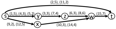
(a) chain DAG	(b) non-chain DAG

Figure 5: Maximum flow computation by greedy

Lemma 1

If $G$ is a chain, the greedy algorithm computes the maximum flow in $G$.

Proof 4.1 (Sketch).

We will prove the lemma by induction. The lemma trivially holds for the base case, when $G$ is a simple edge $(s,t)$. In this case, the greedy algorithm sends to buffer $B_{t}$ the total quantity from all interactions on the edge $(s,t)$ (since $B_{s}=\infty$). Hence, $B_{t}$ has received the maximum possible flow at every time moment. For the inductive step, consider a chain $G$ with the last edge of the chain being $(v,t)$. We will assume that $B_{v}$ has received the maximum possible flow (from the previous vertices of the chain) at any timestamp and prove that $B_{t}$ will receive the maximum possible flow from its incoming edges (i.e., from $v$) at any timestamp. Assume that due to an interaction $(t_{i},q_{i})$ on edge $(v,t)$, instead of applying the greedy algorithm to transfer the maximum possible flow $q=\min\{q_{i},B^{t_{i}}_{v}\}$ from $B^{t_{i}}_{v}$ to $B^{t_{i}}_{t}$, we transfer a smaller quantity $q^{\prime}<q$. We can easily prove that, as a result of this change, the accumulated flow $B_{t}$ at $t$, after processing all interactions cannot increase. The reason is that $t$ receives flow only from $v$, hence, flow reservation by $v$ cannot increase the total flow which will be sent from $v$ to $t$.

We can generalize Lemma 1 and show that the greedy algorithm computes the maximum flow for DAGs where the source is the only vertex which may have more than one outgoing edges.

Lemma 4.2.

Let $G(V,E)$ be a DAG where the source vertex is $s$ and the sink vertex is $t$. The greedy algorithm computes the maximum flow throughout $G$ if for every vertex $v\in V\backslash\{s,t\}$, $v$ has exactly one outgoing edge.

Proof 4.3 (Sketch).

Similarly to the proof of Lemma 1, assume that a vertex $v\in V\backslash\{s,t\}$ having outgoing edge $(v,u)$ does not transfer the maximum possible flow as a result of an interaction $(t_{i},q_{i})$ on $(v,u)$, but retains some quantity. This cannot increase the total quantity that reaches $u$ (and eventually $t$) via $v$ in future interactions $(t_{j},q_{j}),t_{j}>t_{i}$ stemming from $v$ because $(v,u)$ is the only outgoing edge from $v$ and $t$ can be reached from $v$ only via $u$. In addition, there is no benefit in retaining quantities at the source vertex $s$. Hence, greedily transferring the maximum possible quantity at every interaction, results in accumulating the maximum flow at the sink $t$.

Figure 5(b) shows an example, where the Greedy algorithm computes the maximum flow ($=14$). Note that all vertices except for the source $s$ and the sink $t$ have just one outgoing edge. Checking whether the graph satisfies this condition costs just $O(V)$ time, i.e., examining the out-degree of each vertex. On the other hand, we can easily construct examples of graphs that do not satisfy this condition and for which Greedy does not compute the maximum flow (like the graph in Figure 3).

4.2.3 Graph preprocessing

Before applying LP to compute the maximum flow on a DAG for which the Greedy algorithm is not guaranteed to find the maximum flow, i.e., a DAG that does not satisfy the condition of Lemma 4.2, we can reduce the complexity of the problem by removing interactions that do not affect the solution. For example, consider the pattern instance of Figure 2(c) and the last edge $(u_{3},u_{1})$ of this DAG. On this edge, there is an interaction $(1,\$2)$ which obviously does not account in the flow computation and can be ignored. The reason is that the timestamp of this interaction is smaller than all the timestamps of all interactions that enter $u_{3}$, i.e., the source node of interaction $(1,\$2)$. In simple words, it is impossible for $u_{3}$ to transfer $\$2$ at timestamp 1 to $u_{1}$, because by that time it is not possible to have received any money from its incoming interactions. Removing interactions can be crucial to the performance of LP because there are as many variables as the number of interactions in the DAG (except those originating from the source vertex).

Hence, based on the observation above, before applying LP, we perform a preprocessing step on the DAG $G$, where we eliminate interactions that cannot contribute to the maximum flow. Specifically, we consider all vertices of $G$ in a topological order and for each vertex, which is not the source or the sink of the DAG, we examine its outgoing edges and remove from them all interactions with a smaller timestamp than the smallest incoming timestamp to the vertex. The reason of examining the vertices in a topological order is that the deletion of an interaction may trigger the deletion of interactions in edges that follow. Examining the vertices in this order guarantees updating the graph by a single pass over its vertices.

For example, consider the DAG $G_{1}$ shown in Figure 6(a). To preprocess $G_{1}$, we consider its vertices a topological order, i.e., $\{s,x,y,z,t\}$. For each vertex having both incoming and outgoing edges we attempt to delete transactions from its outgoing edges. The first such vertex is $x$. First, we find the minumum timestamp of any incoming interaction to $x$, which is $5$. Then, we examine the interactions on outgoing edge $(x,y)$. From them, interaction $(2,7)$ is deleted because $2<5$. Then, we examine the interactions on outgoing edge $(x,z)$. From them, interaction $(1,2)$ is deleted because $1<5$. We move on to vertex $y$. The minimum timestamp of any interaction entering $y$ is now $9$ (recall that interaction $(2,7)$ on edge $(x,y)$ has been deleted). This causes interaction $(3,3)$ on outgoing edge $(y,t)$ from $y$ to be deleted. Finally, we move on to vertex $z$; the incoming interaction to $z$ with the minimum timestamp is $(10,5)$. This causes interaction $(4,2)$ on outgoing edge $(z,t)$ from $z$ to be deleted. The DAG after preprocessing is shown in Figure 6(b).

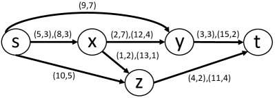
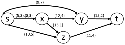
(a) DAG $G_{1}$ before	(b) DAG $G_{1}$ after
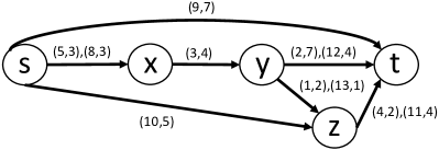
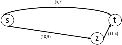
(a) DAG $G_{2}$ before	(b) DAG $G_{2}$ after

Figure 6: DAG preprocessing examples

The DAG preprocessing procedure described above may cause all interactions on an edge to be deleted. In this case, the edge cannot transfer any flow and hence should be deleted. The deletions of edges may result in deletion of nodes and, in turn, trigger the deletion of other edges and nodes. We will now see how the deletion of edges can trigger the simplification of the graph, which can greatly reduce the cost of maximum flow computation.

The deletion of an edge $(v,u)$ may have two effects: (i) the number of incoming edges to vertex $u$ becomes 0, (ii) the number of outgoing edges from vertex $v$ becomes 0. As described above, the deletion of edge $(v,u)$ may happen when we examine vertex $u$. Hence, case (i) can be handled when we examine vertex $u$, which follows $v$ in the topological order. Specifically, if the currently examined vertex $u$ has no incoming edges (the DAG’s source vertex is not examined, hence it is an exception here), then this means that no quantity from the source of the DAG can flow through $u$ to the sink vertex of the DAG. Hence, $u$ and all its outgoing edges should be removed from the DAG. If the removal of an edge $(u,u^{\prime})$ makes its destination vertex $u^{\prime}$ to have no incoming edges, then this outcome will be handled when $u^{\prime}$ will be examined ($u^{\prime}$ must follow $u$ in the topological order).

If, after the deletion of an edge $(v,u)$, case (ii) applies, i.e., $v$ has no more outgoing edges, then this means that no flow can reach the sink of the DAG via $v$. Hence, $v$ and all its incoming edges should be deleted. The deletion of an incoming edge $(w,v)$ may cause vertex $w$ to have no outgoing edges, in which case $w$ should also be deleted. The deletion of $w$ should be done immediately, because $w$ precedes $v$ in the topological order and will not be examined later. The deletion may trigger the deletion of other nodes and edges recursively.

Figures 6(c) and 6(d) show an example of a DAG $G_{2}$ before and after preprocessing. The vertices are examined in topological order $\{s,x,y,z,t\}$. Since $s$ is the source and $t$ is the sink, only vertices $\{x,y,z\}$ are examined in this order. We first examine $x$ and remove the single interaction $(3,4)$ from its outgoing edge $(x,y)$, since $3<\min\{5,8\}$. This causes edge $(x,y)$ to be deleted, which makes $x$ having no outgoing edges. Hence, $x$ and all its incoming edges should be deleted as well. The next vertex to be examined is $y$, which has no incoming edges (since edge $(x,y)$ has been deleted). Hence, $y$ and its outgoing edges are deleted. The next vertex to be examined is $z$ and interaction $(4,2)$ is removed from edge $(z,t)$. The final graph is shown in 6(d). Note that this graph is soluble by Greedy; hence, if DAG preprocessing removes edges from the graph, we apply again the condition of Lemma 4.2 to check if the resulting DAG is soluble by Greedy.

A pseudocode for this DAG preprocessing procedure is Algorithm 1. The algorithm can significantly reduce the size of the problem, by removing interactions, edges, and nodes. In the case where the source or the sink of the DAG is removed, the DAG has 0 flow, which means that we can avoid running the flow computation algorithm. The source vertex can be deleted in the case where the deletion of a vertex propagates upwards until the source. The sink node can be deleted if all its incoming edges are deleted. In any case, after preprocessing, the resulting DAG should be connected and all vertices which are not the source and the sink should have at least one incoming and at least one outgoing edge. The complexity of Algorithm 1 is linear to the number of interactions, as for each examined edge its interactions are processed at most once (from the temporally earliest to the latest) [6]. Each edge is checked for deletion at most twice (once as an outgoing edge and at most once as an incoming edge). Topological sorting of the vertices (in the beginning of the algorithm) examines each edge of the DAG once. Hence, the algorithm is very fast and can potentially result in significant cost savings in maximum flow computation, as we demonstrate in Section 6.

1:DAG $G(V,E)$

2:define topological order for $G$’s vertices

3:for each vertex $v\in V\backslash\{s,t\}$ in topological order do

4:    if $v$ has no incoming edges then

5:         delete all outgoing edges from $v$

6:         delete $v$ from $V$

7:    else

8:         $mintime=\min_{(w,v)\in E}\{\min_{(t,q)\in(w,v)_{S}}t\}$

9:         for each $(v,u)\in E$ do

10:             for each $(t,q)\in(v,u)_{S}$ do

11:                 if $t<mintime$ then

12:                     delete $(t,q)$ from $(v,u)_{S}$

13:                 end if

14:             end for

15:             if $(v,u)_{S}=\emptyset$ then $\triangleright$ all interactions deleted

16:                 delete $(v,u)$ from $E$

17:             end if

18:         end for

19:         if $v$ has no outgoing edges then

20:             delete $v$ from $V$

21:             delete from $E$ all edges $(w,v)$ incoming to $v$ and

22:             recursively delete all $w\in V$ with no outgoing edges

23:         end if

24:    end if

25:end for

Algorithm 1 DAG preprocessing algorithm

4.2.4 Graph simplification

Before applying LP, we also propose a graph simplification approach that can reduce the cost of maximum flow computation. This approach is based on our observation that chains which originate from the source vertex can be reduced to single edges. In a nutshell, graph simplification iteratively identifies and reduces such chains by applying the greedy algorithm on them, until no further reduction can be performed. The resulting graph is then solved using LP.

We start by showing that any chain that starts from the source of the graph can be converted to a single edge without affecting the correctness of maximum flow computation in the graph. The interactions on the single edge that replaces the chain are all interactions that enter the sink (i.e., the destination vertex) of the chain and result in increasing its buffered quantity. For example, the entire chain of Figure 5(a) can be reduced to a single edge $(s,t)$ with interactions $\{(6,3),(8,4)\}$. To derive this edge, we have to run the greedy algorithm on the graph and define one interaction on $(s,t)$ for each interaction $(t_{i},q_{i})$ in $(y,t)$ that increases buffer $B_{t}$. The defined interaction on is $(t_{i},\min\{q_{i},B_{y}^{t_{i}}\})$. Each such interaction corresponds to transferring a quantity from $s=source(G)$ to $t$ through the other nodes. Hence, at any time moment, $B_{t}$ in $G$ is equivalent to $B_{t}$ in the transformed graph. In general, the following lemma holds.

Lemma 4.4.

Let $G$ be an interaction network and let $s$ be the source node of $G$. Assume a chain of $k$ vertices $sv_{1}v_{2}\dots v_{k}$, i.e., for each $v_{i},i<k$, the in- and out-degree of $v_{i}$ is 1. Then, $G$ can then be reduced to a graph $G^{\prime}(V^{\prime},E^{\prime})$, where $V^{\prime}=V-\{v_{1},v_{2},\dots,v_{k-1}\}$ and $E^{\prime}=E-\{(s,v_{1}),(v_{1},v_{2}),\dots,$$(v_{k-1},v_{k})\}+(s,v_{k})$. The interactions on the new edge $(s,v_{k})$ are those that determine the total quantity buffered at $v_{k}$ after running the greedy algorithm on chain $sv_{1}v_{2}\dots v_{k}$. Then, the maximum flow throughout $G$ is equal to the maximum flow throughout $G^{\prime}$.

Proof 4.5 (Sketch).

Recall that reserving flow in the source vertex $s$ of $G$ cannot increase the maximum flow that reaches its sink. The same holds for all vertices $\{v_{1},v_{2},\dots,v_{k-1}\}$ in a chain $sv_{1}v_{2}\dots v_{k}$ that originates from the source $s$, except from the last vertex $v_{k}$. Hence, by running the greedy algorithm and replacing chain$sv_{1}v_{2}\dots v_{k}$ by an edge $(s,v_{k})$ having all interactions that increase buffer $B_{v_{k}}$ does not affect the correctness of maximum flow computation in $G$, as the quantity received by $v_{k}$ via chain $sv_{1}v_{2}\dots v_{k}$ at any time is equivalent to the quantity received by $v_{k}$ via the new edge $(s,v_{k})$ at any time.

Figure 7 illustrates the effect of Lemma 4.4 and exemplifies our simplification approach. Assume that the initial graph is shown in Figure 7(a). After reducing the two chains that originate from the sink to edges, the graph is simplified as shown in Figure 7(b). Note that the reduction of chain $syx$ introduces a new edge $(s,z)$ with interactions $\{(3,2),(7,1)\}$, however, an edge $(s,z)$ already exists in the graph with interactions $\{(2,5),(11,2)\}$. In such a case, the two edges are merged to a single edge with all four interactions as shown in Figure 7(c). After the merging, a new chain $szw$ that originates from the source $s$ is created. This chain is then reduced to single edge $(s,w)$ as shown in Figure 7(d). At this stage the graph cannot be simplified any further, so we compute its maximum flow using LP. Note that the LP optimization problem of the initial graph in Figure 7(a) has 9 variables (as many as the interactions that do not originate from $s$), whereas the reduced graph in Figure 7(d) has only 3 variables. This demonstrates the reduction to the cost of solving the problem achieved by our graph simplification approach.

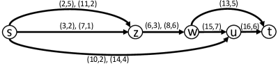
(a) initial graph	(b) first chain reduction
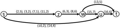
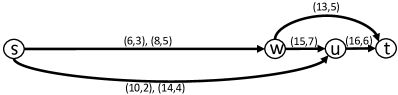
(a) edge merging	(b) second chain reduction

Figure 7: Example of graph simplification

A pseudocode for the proposed graph simplification approach is Algorithm 2. Since each edge is examined just once before being reduced, the complexity of the algorithm is linear to the number of interactions on all edges that are removed (i.e., those processed by executions of the greedy algorithm) and, overall, linear to the number of interactions in the graph. On the other hand, simplification can result in significant cost savings in maximum flow computation, as already discussed and as we demonstrate in Section 6.

1:Graph $G(V,E)$

2:while $G$ contains a chain $C$ originating from source $s$ do

3:    run Greedy to simplify chain $C$ to interaction set $I$

4:    remove edges $\{(s,v_{1}),(v_{1},v_{2}),\dots(v_{2},v_{k})\}$ from $E$

5:    if $\ \textbf{then}(s,v_{k})\notin E$ $\triangleright$ edge $(s,v_{k})$ does not exist

6:         add edge $(s,v_{k})$ to $E$

7:    end if

8:    add $I$ to interaction set of edge $(s,v_{k})$

9:end while

Algorithm 2 Graph simplification algorithm

5 Flow Pattern Enumeration

In the previous section, we have discussed the problem of computing the flow throughout a subgraph of the interaction network. We now turn our attention to flow pattern search in large graphs. As defined in Section 3, a pattern $G_{P}(V_{P},E_{P})$ is a DAG and its instances are subgraphs of the input graph $G(V,E)$. To compute the flow throughout an instance of a pattern, we can use the algorithms presented in Section 4. In this section, we present techniques for finding the pattern instances and their flows. As discussed in Section 2, pattern matching is a well-studied problem, but most previously proposed techniques apply on labeled graphs and all of them disregard flow computation. Our goal here is to demonstrate that the enumeration of pattern instances and their flows in an interaction network can greatly benefit from a simple graph preprocessing technique. Before discussing it, we present a baseline graph browsing approach.

5.1 A graph browsing approach

A direct approach to solve the pattern search problem traverses the graph, trying to identify matches of the pattern $G_{P}$ by expanding partial matches of $G_{P}$. As discussed in previous work [32], graph browsing could be the most efficient approach, especially for pattern search in unlabeled graphs, where the number of instances can be numerous. Specifically, in graph browsing, the vertices of $G_{P}$ are considered in a topological order. Starting from the source vertex of $G_{P}$, for each vertex $v_{P}\in G_{P}$, $v_{P}$ is mapped to a vertex $v\in G$, making sure that all structural and mapping ($\mu$) constraints w.r.t. all previously instantiated vertices are satisfied. For example, consider the pattern $G_{P}$ of Figure 2(b) and the graph $G$ of Figure 2(a). To find all matches of $G_{P}$ in $G$, we instantiate the first vertex $a$ of $G_{P}$ to each of the four vertices of $G$ and for each instance of $a$, we perform graph browsing to gradually “complete” possible matches (using a backtracking algorithm). That is, from $a=u_{1}$, we follow the outgoing edge of $u_{1}$ to instantiate $b=u_{2}$; then, the outgoing edge of $b=u_{2}$ to instantiate $c=u_{3}$; then, the first outgoing edge of $c=u_{3}$ to instantiate the sink vertex $a=u_{1}$, which gives us the pattern match $u_{1}u_{2}u_{3}u_{1}$. Then, we backtrack and try the instantiation $a=u_{4}$, which fails, because $u_{4}\neq u_{1}$ (recall that $u_{1}$ is already mapped to the source $a$ of $G_{M}$). For each pattern instance computed by this method, we can use the approaches proposed in Section 4 to compute the corresponding flow.

Note that for certain patterns, like the chain pattern of Figure 2(b), for which the maximum flow can be computed by the greedy algorithm, we can compute the maximum flows of their instances by gradually computing the interactions that determine the maximum flows of their partial matches (similarly to the simplification approach that we have proposed in Section 4.2.4). For example, after finding the partial match $u_{1}u_{2}u_{3}$, we apply the greedy approach to derive the set of interactions $\{(3,\$4),(5,\$2)\}$, which determine the maximum flow into $u_{3}$ originating from $u_{1}$ at any time moment. After we expand to complete the match $u_{1}u_{2}u_{3}u_{1}$, we can compute its flow incrementally, from the set of interactions $\{(3,\$4),(5,\$2)\}$ into $u_{3}$, by using only this set and the interactions on edge $u_{3}u_{1}$ in the greedy algorithm. If $u_{1}u_{2}u_{3}$ was expanded to another pattern match, we could still use the same set $\{(3,\$4),(5,\$2)\}$ to compute its flow incrementally, without having to run the greedy algorithm for the entire set of interactions in the new instance.

The advantage of the graph browsing pattern enumeration approach is that it is a general method that does not require any precomputed information. At the same time, it is expected to be reasonably efficient, because there is not much room for pruning vertices as not being candidates to be mapped to pattern vertices (recall that graph vertices are unlabeled and mapping is only based on equality/inequality constraints to other mapped vertices). In the next subsection, we propose a graph preprocessing approach that facilitates faster pattern enumeration.

5.2 A preprocessing-based approach

We assume that the graph $G$ is static (i.e., it contains historical data). We propose the preprocessing of $G$ and the extraction from it instances of certain subgraphs that can help in identifying instances of larger patterns that include the subgraphs. The intuition behind this approach is that we can avoid searching for subgraphs of the pattern from scratch; instead, we can retrieve the pattern’s structural components (and precomputed flow data) and then “stitch” them together using join algorithms. This is not a new idea, as the extraction and indexing of subgraphs in order to facilitate graph pattern search has been used in several studies [32, 5]. Here, we employ the idea in the context of flow pattern enumeration.

Path Precomputation. The subgraphs we precompute are paths up to a certain length (i.e., up to $k$ hops). We form one table for each length, holding all paths of that length. That is, for each path, we store: (i) the sequence of vertex-ids that form the path, (ii) the sequence of interactions $e_{S}$ that enter the buffer $B_{t}$ of the sink $t$ of the path, after applying the greedy algorithm; $e_{S}$ determines the flow from the source of the path to the sink at any time moment.

Enumeration of Pattern Instances. To enumerate all pattern instances using the precomputed tables, the first step is to identify precomputed path subpatterns in $G_{P}$ and access and join the corresponding tables, in order to form either complete instances of $G_{P}$, or partial ones if complete instances cannot be derived simply by combining paths from the accessed tables. In the latter case, we use the graph representation to verify the existence of any missing edges in the partial instance and/or to expand from the partial instances and include missing vertices and edges (or determine that the partial instance cannot be expanded to a complete one). As soon as a complete pattern match is identified, we compute the flow of the graph. While doing so, we use any precomputed flows from the tables wherever possible to avoid flow computations.

Consider, for example, the flow pattern $G_{P}$ shown in Figure 8(a). Assume that we have preprocessed and have available all instances of two-hop and three-hop cyclic paths that start from and end to the same node $a$ in two tables $L_{2}$ and $L_{3}$, respectively. In this case, we can easily compute all instances of $G_{P}$, by only accessing and using preprocessed data. Specifically, if the preprocessed paths are sorted by vertex-id, it suffices to scan $L_{2}$ and $L_{3}$ and merge-join them, in order to find all pairs of paths from $L_{2}$ and $L_{3}$ that have the same start (and hence end) vertex. For each such pair, we verify the remaining constraint (that $b$ and $c$ are mapped to vertices different than the one whereto $e$ is mapped). Finally, to compute the total flow of the resulting pattern instance, we sum up all precomputed incoming flows to the sinks of the two paths.

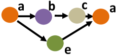
(a) easy pattern	(b) hard pattern

Figure 8: Examples of flow patterns

On the other hand, the precomputed data may not be fully utilizable, when computing the instances of patterns such as the one in Figure 8(b). To enumerate the instances of such a pattern, we can first scan the $L_{3}$ table and for each accessed 3-hop cycle $\mu(a)\to\mu(b)\to\mu(c)\to\mu(a)$, access the input graph $G(V,E)$ to verify whether there is an edge that connects the vertex $\mu(a)\in V$ mapped to $a$ to the vertex $\mu(c)\in V$ mapped to $c$ and whether there is an edge that connects the vertex $\mu(b)\in V$ mapped to $b$ to the vertex $\mu(a)\in V$ mapped to $a$. If these edges do exist, they are retrieved and combined with the edges along the path $\mu(a)\to\mu(b)\to\mu(c)\to\mu(a)$ to form an instance, which is then passed to the algorithms of Section 4 for flow computation. In this case, the precomputed flows of paths in $L_{3}$ cannot be used because the paths are not isolated in the instances of the pattern.

In general, precomputed flows along paths can be useful only for pattern instances wherein these paths are independent and can be progressively simplified using the technique proposed in Section 4.2.4. Still, even when precomputed flows are not useful, the precomputed paths can be used to accelerate finding the instances of the patterns.

We have assumed so far that the precomputed path tables are sorted by starting vertex (and by prefix in general). This helps to reduce the cost of pattern matching by merge-joining the tables. If the number of path instances is not extreme, tables can also be sorted by other columns or column indices can be used to accelerate other cases of joins. In addition, it is possible to use hash tables for each of the columns and replace joins by lookups.

5.3 Non-rigid patterns

The patterns that we have defined so far have a rigid structure which is determined by a DAG. In some applications, however, certain patterns with more relaxed structure could be of interest. Consider, for example, a money-laundering pattern where a source node $a$ is sending payments to recipients (which do not have a fixed number) and then these recipients send money back to $a$. We might be interested in identifying instances of such patterns and their corresponding flows. Right now, we could only define a set of different patterns and measure their flows independently, as shown in Figure 9(a). Then, we could aggregate the flows of all instances of the different patterns that correspond to the same node $a$ in order to compute the total flow from $a$ to $a$ via other nodes.

This approach has several shortcomings. First, we would have to compute and merge the results of multiple pattern queries. Second, there is no limit on how many patterns we should use. Third, the final result might not be correct, as the flows of subpatterns could be included in the flows of superpatterns (for example, an instance of the 2nd pattern in Figure 9(a) includes two instances of the first pattern).

In order to avoid these issues, we can define a relaxed pattern as shown in Figure 9(b), which links $a$ to $a$ by parallel paths via any number of intermediate nodes. Finding the instances of this pattern and measuring their flows is very easy using our precomputation approach, as we only have to scan the 2-hop cycle table $L_{2}$ and, for each instance of $a$, we have to aggregate the flows of the corresponding rows of the table. We can also set constraints to the number of paths in a non-rigid pattern. For example, we may be interested in instances of the pattern shown in Figure 9(b) which include at least 10 cycles.

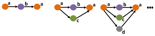
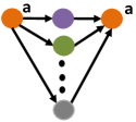
(a) 2-hop rigid patterns	(b) relaxed pattern

Figure 9: 2-hop nonrigid pattern

6 Experimental Evaluation

In this section, we evaluate the performance of the flow computation techniques proposed in Section 4. In addition, we evaluate the efficiency of the preprocessing-based approach for flow pattern enumeration proposed in Section 5. All methods were implemented in C and the experiments were run on a MacBook Pro with an 2.3 GHz Quad-Core Intel Core i5 and 8GB memory. For the implementation of LP, we used the lpsolve library (version 5.5.2.5). The source code of the paper is publicly available.

6.1 Description of Datasets

We used three real datasets, generated from real interaction networks: the Bitcoin transactions network, an internet traffic network and a loans exchange network. We now provide details about the data. Table 4 summarizes statistics about them.

Bitcoin: We downloaded all transactions in the bitcoin network [25] up to 2013.12.28 from http://www.vo.elte.hu/bitcoin/. The data were collected and formatted by the authors of [17]. We joined tables ‘txedge.txt’ with ‘txout.txt’ to create a single table with transactions of the form (sender, recipient, timestamp, amount). We also used table ‘contraction.txt’ to merge addresses which belong to the same user. Addresses were mapped to integers in a continuous range starting from 0. Finally, we converted all amounts to B    (originally in Satoshis, where 1 Satoshi=$10^{-8}$ B   ) and removed all insignificant transactions with amounts less than 10000 Satoshis.

CTU-13: We extracted data from a botnet traffic network , created in CTU University[10]. Hence, the vertices of the graph are IP addresses and the interactions are data exchanges between them at different timestamps. We consider as flow the total amount of bytes transferred between IP addresses.

Prosper Loans: Prosper is an online peer-to-peer loan service. We consider Prosper as an interaction network between users who lend money to each other. Each record includes the lender, the borrower, the time of the transaction and the loan amount. We disregarded the tax that the borrower paid for the transaction and considered only the net loan amount. The data were downloaded from http://konect.uni-koblenz.de.

Table 4: Characteristics of Datasets

Dataset	#nodes	#edges	#interactions	avg. flow
Bitcoin	12M	27.7M	45.5M	34.4 B
CTU-13	607K	697K	2.8M	19.2KB
Prosper Loans	88K	3M	3.04M	$\$$76

6.2 Flow Computation

In the first set of experiments, we evaluate the flow computation techniques discussed in Section 4. For this purpose, we extracted a number of subgraphs from each network and we applied flow computation on each of them. Specifically, we identified seed vertices in the networks from which there are paths (up to three hops) that pass through other vertices and then return to the origin. For each seed vertex, we merged all edges along these paths to form a single subgraph of the network. Figure 10 shows an example of such a subgraph, formed by merging all paths that start from vertex 143 and end at the same vertex.

Figure 10: Example of a subgraph extracted from Bitcoin

We discarded subgraphs with more than 10K interactions because the LP algorithm for maximum flow computation was too slow on them. The number of tested subgraphs extracted from each dataset and their statistics are shown in Table 5. The subgraphs are relatively small in terms of vertices and edges, but they have a large average number of interactions (compared to the expected number derived from Table 4). Hence, (i) these subgraphs are statistically interesting, because they have many interactions and relatively large flow and (ii) computing the maximum flow through them is relatively expensive (again, due to the large number of interactions).

Table 5: Statistics of subgraphs

Dataset	#subgraphs	avg #vertices	avg #edges	avg #interactions
Bitcoin	48.7K	5.16	6.42	448.4
CTU-13	9235	3.24	2.49	15.9
Prosper Loans	137	6.1	8	611.5

Compared methods. We applied the following methods to compute the flow on the extracted subgraphs from each dataset.

• The greedy algorithm presented in Section 4.1. This algorithm is naturally the fastest one, but computes the flow based on the greedy transfer assumption, i.e., it does not (always) find the maximum flow that can be transferred from the source to the sink of the graph.

• LP solves the maximum flow problem using linear programming, as discussed in Section 4.2, using a direct application of the LP solver.

• Pre first applies the greedy solubility test on the subgraph (explained in Section 4.2.2) to test whether the maximum flow can be computed using the greedy algorithm. In this case, it uses the greedy algorithm instead of LP. Otherwise, it applies the graph preprocessing approach (Section 4.2.3) to remove any interactions, edges, or vertices that do not contribute to flow computation. If any edges and/or vertices are removed, it checks again for solubility by greedy. In the end, if the maximum flow is not guaranteed to be computed by greedy, it applies LP.

• PreSim follows the steps of Pre and if, in the end, LP has to be applied, PreSim attempts to further simplify the graph by applying the method presented in Section 4.2.4 which computes part of the maximum flow using the greedy algorithm. PreSim is our complete solution for maximum flow computation in temporal interaction networks.

Results. The second rows of Tables 6, 7, and 8 show the average runtime (in msec) of the compared flow computation methods per tested subgraph. The greedy algorithm is lightning fast, as its cost is linear to the number of interactions. Its running time in all cases is in the order of microseconds. For the maximum flow problem, the baseline LP approach is very slow especially on the Bitcoin subgraphs, which contain the largest number of interactions on average (see Table 5). With the help of the preprocessing approach (Pre), the graphs are simplified and the cost of maximum flow computation is reduced up to 14 times compared to LP. Note that the time for preprocessing the graphs is included in the measured runtimes. Finally, the graph simplification method (PreSim) further reduces the cost at least two times compared to Pre. On average, the speedup of our proposed maximum flow computation approach (PreSim) over LP is 11x, 13x, and 32x on three networks.

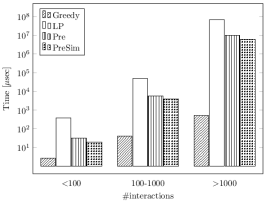
(a) Bitcoin Network

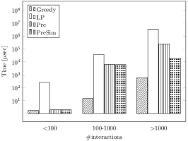
(b) Botnet Network

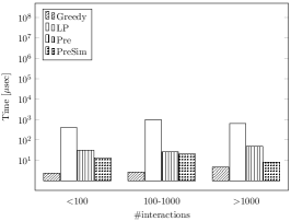
(c) Prosper Loans Network

​​​​ ​​​​

Figure 11: Runtime of algorithms as a function of the number of interactions

For a more detailed analysis of the results, we divided the tested subgraphs in three classes. Class A contains the easiest subgraphs, which are found to be soluble by the greedy method. As explained before, the cost of verifying whether a graph is soluble is very low, so the cost of computing the maximum flow on these graphs equals the cost of running the greedy algorithm. Class B contains the subgraphs, which are found to be soluble by greedy after they have been simplified by preprocessing. The cost for computing the maximum flow on these graphs is again close to that of the greedy algorithm. Finally, class C contains the hardest graphs, which even after preprocessing cannot be solved using the greedy algorithm. The last three rows of Tables 6–8 average the runtimes of the tested methods on each of the three classes of subgraphs.

We also divided the tested subgraphs into three categories based on the number of interactions they include (less than 100 interactions, between 100 and 1000 interactions, more than 1000 interactions). Figure 11 compares the average performance of all methods on each category of subgraphs at each dataset. As expected, the costs of all methods increase with the number of interactions. In general, the savings of PreSim and Pre over LP are not affected by the magnitude of the problem size. Overall, the experiments confirm the efficiency of the proposed techniques in Section 4 for greedy and maximum flow computation.

Table 6: Runtime (msec) for Bitcoin subgraphs

	Greedy	LP	Pre	PreSim
All (48.7K)	0.0491	5775	838.8	524.5
Class A (35.4K)	0.0074	2667.18	0.0078	0.0078
Class B (7891)	0.295	7179.39	0.575	0.575
Class C (5366)	0.353	24248	7615.8	4762.43

Table 7: Runtime (msec) for CTU-13 subgraphs

	Greedy	LP	Pre	PreSim
All (9235)	0.0035	10.313	6.314	0.7902
Class A (9199)	0.0032	3.835	0.0033	0.0033
Class B (3)	0.0037	71.07	0.0074	0.0074
Class C (33)	0.0757	1810.38	1767.5	220.2

Table 8: Runtime (msec) for Prosper Loans subgraphs

	Greedy	LP	Pre	PreSim
All (137)	0.0027	0.5105	0.0352	0.0157
Class A (94)	0.0015	0.5072	0.0016	0.0016
Class B (25)	0.004	0.5646	0.008	0.008
Class C (18)	0.0067	0.4527	0.2373	0.0889

6.3 Pattern Search

We now evaluate the flow pattern enumeration approaches presented in Section 5. Specifically, we compare the time that the graph browsing (GB) approach (Section 5.1) and the preprocessing-based (PB) approach (Section 5.2) need to find the instances of several simple graph patterns and to compute the maximum flow of each instance. We constructed main-memory representations of the three interaction networks that facilitate graph browsing (i.e., we can navigate to the neighbors of each vertex with the help of adjacency lists).

Due to the high precomputation and storage cost, from datasets Bitcoin and CTU-13, we were able to precompute and store only paths up to 3 hops where the start and the end vertex are the same (i.e., cycles). Paths of longer sizes and of arbitrary nature are multiple times larger than the original datasets. On the other hand, the precomputed cycles up to three hops require at most 20% space compared to the size of the entire graphs. For the Prosper Loans dataset, we also precomputed 2-hop chains (i.e., paths of three different nodes) which could easily be accommodated in the main memory of our machine.

Figure 12 shows the set of patterns that we tested in the experiments. We experimented with six rigid patterns (P1–P6) and three relaxed (non-rigid) patterns (RP1–RP3). In the non-rigid patterns (see Section 5.3), all vertices in the parallel paths (except for the source and the sink) are required to be different.

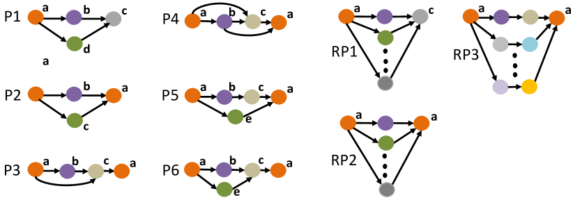
Figure 12: Set of tested patterns

Tables 9, 10, and 11 compare the performance of GB to that of PB on enumerating the instances of the various patterns and computing their maximum flow. Note that for Bitcoin and CTU-13 datasets, the processing times for P1 and RP1 were not included because PB was not applicable in this case (we have not precomputed any path that would be useful). In general, we observe that preprocessing pays off in most of the tested patterns, as the runtimes of PB in most cases are at least one order of magnitude lower than the corresponding ones of GB.

For some patterns and networks, prepcocessing (PB) does not give much benefit compared to GB. For example, for pattern P4 on the Bitcoin network (marked with *), search by both GB and PB was terminated after finding the first 3000 instances, because both methods are extremely slow. The preprocessed flows cannot be used and the maximum flow of the instances must be computed by LP. Hence, on the Bitcoin network, PB has a similar cost as GB, as the instances contain numerous interactions and maximum flow computation dominates the overall cost of pattern enumeration. The same holds for P6 (again on Bitcoin), which was terminated earlier because both methods were quite slow.

Table 9: Pattern Search on Bitcoin

Pattern	Instances	Average flow	GB	PB
P2	22.3G	56.15	23.2 hours	30.59 sec
P3	2.8M	4786.18	3155.96 sec	179.70 sec
P4*	3000	697.04	446.73 sec	421.85 sec
P5	577.5M	8069.2	15 days (est.)	179.74 sec
P6*	2.04T	2.81	1445 sec	1059 sec
RP2	655K	39.86	422.79 sec	53.273 msec
RP3	1.2M	1.86	306 min	13.53 msec

Table 10: Pattern Search on CTU-13

Pattern	Instances	Average flow	GB	PB
P2	709M	2888.90	1952.61 sec	762.65 msec
P3	182	528.5K	55.71 sec	8.61 msec
P4	91	1.56M	58.564 sec	2.518 sec
P5	208K	13116.5	443.97 sec	4.73 msec
P6	586	52892	410.4 sec	14.87 msec
RP2	51266	11942.65	24.15 sec	0.63 msec
RP3	91	61485.58	375.39 sec	0.035 msec

Table 11: Pattern Search on Prosper Loans

Pattern	Instances	Average flow	GB	PB
P1	5.12M	45.89	119.08 sec	2.80 sec
P2	201	223.23	88.66 msec	0.004 msec
P3	268	100.44	3.57 sec	1.3 msec
P4	98	299.55	3.54 sec	0.723 msec
P5	1833	121.47	605.67 msec	0.021 msec
P6	1296	43.55	474.61 msec	11.13 msec
RP1	25.5M	25.12	133.37 sec	3.01 sec
RP2	260	58.061	0.016 msec	0.004 msec
RP3	532	10.94	503.89 msec	0.040 msec

7 Conclusions

In this paper we defined and studied the problem of flow computation in interaction networks. We defined two models for flow computation, one based on greedy flow transfer between vertices and one that assumes arbitrary flow transfer and the objective is to compute the maximum flow. We showed that flow computation based on the first model can be conducted very efficiently, whereas the more interesting maximum flow computation is more expensive. In view of this, we proposed and evaluated a number of techniques to reduce the cost of maximum flow computation by at least one order of magnitude. Note that our techniques are readily applicable for the time-restricted version of the problem, where we are only interested in interactions that happen within a time window (i.e., by simply disregarding all interactions that happened outside the window). Finally, we studied the problem of pattern enumeration in large graphs, where for each pattern instance, we also have to compute the maximum flow. For this problem we proposed a technique that precomputes the instances of simple subgraphs and their flows and uses them to accelerate the finding of more complex patterns that have these subgraphs as components.

Directions for future work include (i) the investigation of additional techniques for reducing the cost of the maximum flow problem, (ii) the investigation of similar simplification techniques to other flow computation problems, and (iii) the automatic identification of interesting patterns and subgraphs that have significantly more flow than expected.

References

- [1] R. K. Ahuja, T. L. Magnanti, and J. B. Orlin. Network Flows: Theory, Algorithms, and Applications. Prentice hall, 1993.
- [2] E. C. Akrida, J. Czyzowicz, L. Gasieniec, L. Kuszner, and P. G. Spirakis. Temporal flows in temporal networks. In CIAC, pages 43–54, 2017.
- [3] N. Baumann and M. Skutella. Earliest arrival flows with multiple sources. Mathematics of Operations Research, 34(2):499–512, 2009.
- [4] O. Y. Chén, H. Cao, J. M. Reinen, T. Qian, J. Gou, H. Phan, M. D. Vos, and T. D. Cannon. Resting-state brain information flow predicts cognitive flexibility in humans. Nature Scientific Reports, 9(3879), 2019.
- [5] J. Cheng, J. X. Yu, B. Ding, P. S. Yu, and H. Wang. Fast graph pattern matching. In ICDE, pages 913–922, 2008.
- [6] T. H. Cormen, C. E. Leiserson, R. L. Rivest, and C. Stein. Introduction to algorithms. MIT press, 2009.
- [7] J. Edmonds and R. M. Karp. Theoretical improvements in algorithmic efficiency for network flow problems. J. ACM, 19(2):248–264, 1972.
- [8] L. R. Ford and D. R. Fulkerson. Maximal flow through a network. Canadian Journal of Mathematics, (8):399–404, 1956.
- [9] B. Gallagher. Matching structure and semantics: A survey on graph-based pattern matching. In AAAI Fall Symposium: Capturing and Using Patterns for Evidence Detection, pages 45–53, 2006.
- [10] S. Garcia, M. Grill, J. Stiborek, and A. Zunino. An empirical comparison of botnet detection methods. Computers & Security, 45:100–123, 2014.
- [11] A. V. Goldberg and R. E. Tarjan. Efficient maximum flow algorithms. Communications of the ACM, 57(8):82–89, 2014.
- [12] S. Gurukar, S. Ranu, and B. Ravindran. COMMIT: A scalable approach to mining communication motifs from dynamic networks. In SIGMOD, pages 475–489, 2015.
- [13] H. W. Hamacher and S. A. Tjandra. Earliest arrival flows with time-dependent data. Technische Universität Kaiserslautern, 2003.
- [14] P. Holme and J. Saramäki. Temporal networks. CoRR, abs/1108.1780, 2011.
- [15] B. Hoppe. Efficient dynamic network flow algorithms. Technical report, Cornell University, 1995.
- [16] D. Kondor, I. Csabai, J. Szüle, M. Pósfai, and G. Vattay. Inferring the interplay between network structure and market effects in bitcoin. New Journal of Physics, 16(12):125003, 2014.
- [17] D. Kondor, M. Pósfai, I. Csabai, and G. Vattay. Do the rich get richer? an empirical analysis of the bitcoin transaction network. PLoS ONE, 9(2):e86197, 2013.
- [18] C. Kosyfaki, N. Mamoulis, E. Pitoura, and P. Tsaparas. Flow motifs in interaction networks. In EDBT, pages 241–252, 2019.
- [19] R. Kumar and T. Calders. Information propagation in interaction networks. In EDBT, pages 270–281, 2017.
- [20] R. Kumar and T. Calders. 2scent: An efficient algorithm to enumerate all simple temporal cycles. PVLDB, 11(11):1441–1453, 2018.
- [21] M. Kuramochi and G. Karypis. Frequent subgraph discovery. In IEEE International Conference on Data Mining, pages 313–320, 2001.
- [22] M. Kuramochi and G. Karypis. Finding frequent patterns in a large sparse graph. Data mining and knowledge discovery, 11(3):243–271, 2005.
- [23] S. Meiklejohn, M. Pomarole, G. Jordan, K. Levchenko, D. McCoy, G. M. Voelker, and S. Savage. A fistful of bitcoins: characterizing payments among men with no names. In IMC 2013,, pages 127–140. ACM, 2013.
- [24] R. Milo, S. Shen-Orr, S. Itzkovitz, N. Kashtan, D. Chklovskii, and U. Alon1. Network motifs: Simple building blocks of complex networks. Science, 298(5594):824–827, 2004.
- [25] S. Nakamoto. Bitcoin: A peer-to-peer electronic cash system http://bitcoin.org/bitcoin.pdf, 2007.
- [26] A. Paranjape, A. R. Benson, and J. Leskovec. Motifs in temporal networks. In WSDM, pages 601–610, 2017.
- [27] S. Ranu and A. K. Singh. Graphsig: A scalable approach to mining significant subgraphs in large graph databases. In ICDE, pages 844–855, 2009.
- [28] U. Redmond and P. Cunningham. Subgraph isomorphism in temporal networks. CoRR, abs/1605.02174, 2016.
- [29] S. Ruzika, H. Sperber, and M. Steiner. Earliest arrival flows on series-parallel graphs. Networks, 57(2):169–173, 2011.
- [30] K. Semertzidis and E. Pitoura. Durable graph pattern queries on historical graphs. In ICDE, pages 541–552, 2016.
- [31] M. Skutella. An introduction to network flows over time. In Bonn Workshop of Combinatorial Optimization, 2008.
- [32] Z. Sun, H. Wang, H. Wang, B. Shao, and J. Li. Efficient subgraph matching on billion node graphs. PVLDB, 5(9):788–799, 2012.
- [33] L. Zou, L. Chen, and M. T. Özsu. Distance-join: Pattern match query in a large graph database. Proceedings of the VLDB Endowment, 2(1):886–897, 2009.
- [34] A. Züfle, M. Renz, T. Emrich, and M. Franzke. Pattern search in temporal social networks. In EDBT, pages 289–300, 2018.