A Mean Field Game price model with noise

Abstract.

In this paper, we propose a mean-field game model for the price formation of a commodity whose production is subjected to random fluctuations. The model generalizes existing deterministic price formation models.

Agents seek to minimize their average cost by choosing their trading rates with a price that is characterized by a balance between supply and demand. The supply and the price processes are assumed to follow stochastic differential equations.

Here, we show that, for linear dynamics and quadratic costs, the optimal trading rates are determined in feedback form. Hence, the price arises as the solution to a stochastic differential equation, whose coefficients depend on the solution of a system of ordinary differential equations.

1. Introduction

Mean-field games (MFG) is a tool to study the Nash equilibrium of infinite populations of rational agents. These agents select their actions based on their state and the statistical information about the population. Here, we study a price formation model for a commodity traded in a market under uncertain supply, which is a common noise shared by the agents. These agents are rational and aim to minimize the average trading cost by selecting their trading rate. The distribution of the agents solves a stochastic partial differential equation. Finally, a market-clearing condition characterizes the price.

We consider a commodity whose supply process is described by a stochastic differential equation; that is, we are given a drift $b^{S}:[0,T]\times{\mathbb{R}}^{2}\to{\mathbb{R}}$ and volatility $\sigma^{S}:[0,T]\times{\mathbb{R}}^{2}\to{\mathbb{R}}^{+}_{0}$, which are smooth functions, and the supply $Q_{s}$ is determined by the stochastic differential equation

$$dQ_{s}=b^{S}(Q_{s},\varpi_{s},s)ds+\sigma^{S}(Q_{s},\varpi_{s},s)dW_{s}\quad\mbox{ in }[0,T]$$ (1.1)

with the initial condition $\bar{q}$. We would like to determine the drift $b^{P}:[0,T]\times{\mathbb{R}}^{2}\to{\mathbb{R}}$, the volatility $\sigma^{P}:[0,T]\times{\mathbb{R}}^{2}\to{\mathbb{R}}^{+}_{0}$, and $\bar{w}$ such that the price $\varpi_{s}$ solves

$$d\varpi_{s}=b^{P}(Q_{s},\varpi_{s},s)ds+\sigma^{P}(Q_{s},\varpi_{s},s)dW_{s}\quad\mbox{ in }[0,T]$$ (1.2)

with initial condition $\bar{w}$ and such that it ensures a market clearing condition. It may not be possible to find $b^{P}$ and $\sigma^{P}$ in a feedback form. However, for linear dynamics, as we show here, we can solve quadratic models, which are of great interest in applications.

Let ${\bf X}_{s}$ be the quantity of the commodity held by an agent at time $s$ for $t\leqslant s\leqslant T$. This agent trades this commodity, controlling its rate of change, ${\bf v}$, thus

$$d{\bf X}_{s}={\bf v}(s)ds~{}~{}\mbox{ in }[t,T].$$ (1.3)

At time $t$, an agent who holds $x$ and observes $q$ and $w$ chooses a progressively measurable control process ${\bf v}$ to minimize the expected cost functional

$$J(x,q,w,t;{\bf v})={\mathds{E}}\left[\int_{t}^{T}L({\bf X}_{s},{\bf v}(s))+\varpi_{s}{\bf v}(s)ds+\Psi\left({\bf X}_{T},Q_{T},\varpi_{T}\right)\right],$$ (1.4)

subject to the dynamics (1.1), (1.2), and (1.3) with initial condition ${\bf X}_{t}=x$, and the expectation is taken w.r.t. the standard filtration generated by the Brownian motion. The Lagrangian, $L$, takes into account costs such as market impact or storage, and the terminal cost $\Psi$ stands for the terminal preferences of the agent.

This control problem determines a Hamilton-Jacobi equation addressed in Section 2.1. In turn, each agent selects an optimal control and uses it to adjust its holdings. Because the source of noise in $Q_{t}$ is common to all agents, the evolution of the probability distribution of agents is not deterministic. Instead, it is given by a stochastic transport equation derived in Section 2.2. Finally, the price is determined by a market-clearing condition that ensures that supply meets demand. We study this condition in Section 2.3.

Mathematically, the price model corresponds to the following problem.

Problem 1.

Given a Hamiltonian, $H:{\mathbb{R}}^{2}\to{\mathbb{R}}$, $H\in C^{\infty}$, a commotity’s supply initial value, $\bar{q}\in{\mathbb{R}}$, supply drift, $b^{S}:{\mathbb{R}}^{2}\times[0,T]\to{\mathbb{R}}$, and supply volatility, $\sigma^{S}:{\mathbb{R}}^{2}\times[0,T]\to{\mathbb{R}}$, a terminal cost, $\Psi:{\mathbb{R}}^{3}\to{\mathbb{R}}$, $\Psi\in C^{\infty}({\mathbb{R}}^{3})$, and an initial distribution of agents, $\bar{m}\in C^{\infty}_{c}({\mathbb{R}})\cap{\mathcal{P}}({\mathbb{R}})$, find $u:{\mathbb{R}}^{3}\times[0,T]\to{\mathbb{R}}$, $\mu\in C([0,T],{\mathcal{P}}({\mathbb{R}}^{3}))$, $\bar{w}\in{\mathbb{R}}$, the price at $t=0$, the price drift $b^{P}:{\mathbb{R}}^{2}\times[0,T]\to{\mathbb{R}}$, and the price volatility $\sigma^{P}:{\mathbb{R}}^{2}\times[0,T]\to{\mathbb{R}}$ solving

$$\begin{cases}-u_{t}+H(x,w+u_{x})=b^{S}u_{q}+b^{P}u_{w}+\tfrac{1}{2}(\sigma^{S})^{2}u_{qq}+\sigma^{S}\sigma^{P}u_{qw}+\tfrac{1}{2}(\sigma^{P})^{2}u_{ww}\\ d\mu_{t}=\left(\left(\mu\tfrac{(\sigma^{S})^{2}}{2}\right)_{qq}+(\mu\sigma^{S}\sigma^{P})_{qw}+\left(\mu\tfrac{(\sigma^{P})^{2}}{2}\right)_{ww}-\operatorname{div}(\mu{\bf b})\right)dt-\operatorname{div}(\mu{\boldsymbol{\sigma}})dW_{t}\\ \int_{{\mathbb{R}}^{3}}q+D_{p}H(x,w+u_{x}(x,q,w,t))\mu_{t}(dx\times dq\times dw)=0,\end{cases}$$ (1.5)

and the terminal-initial conditions

$$\begin{cases}u(x,q,w,T)=\Psi(x,q,w)\\ \mu_{0}=\bar{m}\times\delta_{\bar{q}}\times\delta_{\bar{w}},\end{cases}$$ (1.6)

where ${\bf b}=(-D_{p}H(x,w+u_{x}),b^{S},b^{P})$, ${\boldsymbol{\sigma}}=(0,\sigma^{S},\sigma^{P})$, and the divergence is taken w.r.t. $(x,q,w)$.

Given a solution to the preceding problem, we construct the supply and price processes

$$Q_{t}=\int_{{\mathbb{R}}^{3}}q~{}\mu_{t}(dx\times dq\times dw)$$

and

$$\varpi_{t}=\int_{{\mathbb{R}}^{3}}w~{}\mu_{t}(dx\times dq\times dw),$$

which also solve

$$\begin{cases}dQ_{t}&=b^{S}(Q_{t},\varpi_{t},t)dt+\sigma^{S}(Q_{t},\varpi_{t},t)dW_{t}\quad\mbox{ in }[0,T]\\ d\varpi_{t}&=b^{P}(Q_{t},\varpi_{t},t)dt+\sigma^{P}(Q_{t},\varpi_{t},t)dW_{t}\quad\mbox{ in }[0,T]\end{cases}$$

with initial conditions

$$\begin{cases}Q_{0}=\bar{q}\\ \varpi_{0}=\bar{w}\end{cases}$$ (1.7)

and satisfy the market-clearing condition

$$Q_{t}=\int_{{\mathbb{R}}}-D_{p}H(x,\varpi_{t}+u_{x}(x,Q_{t},\varpi_{t},t))\mu_{t}(dx).$$

In [10], the authors presented a model where the supply for the commodity was a given deterministic function, and the balance condition between supply and demand gave rise to the price as a Lagrange multiplier. Price formation models were also studied by Markowich et al. [18], Caffarelli et al. [2], and Burger et al. [1]. The behavior of rational agents that control an electric load was considered in [17, 16]. For example, turning on or off space heaters controls the electric load as was discussed in [14, 15, 13]. Previous authors addressed price formation when the demand is a given function of the price [12] or that the price is a function of the demand, see, for example [6], [5], [7], [8], and [11]. An $N$-player version of an economic growth model was presented in [9].

Noise in the supply together with a balance condition is a central issue in price formation that could not be handled directly with the techniques in previous papers. A probabilistic approach of the common noise is discussed in Carmona et al. in [4]. Another approach is through the master equation, involving derivatives with respect to measures, which can be found in [3]. None of these references, however, addresses problems with integral constraints such as (1.7).

Our model corresponds to the one in [10] for the deterministic setting when we take the volatility for the supply to be 0. Here, we study the linear-quadratic case, that is, when the cost functional is quadratic, and the dynamics (1.1) and (1.2) are linear. In Section 3.2, we provide a constructive approach to get semi-explicit solutions of price models for linear dynamics and quadratic cost. This approach avoids the use of the master equation. The paper ends with a brief presentation of simulation results in Section 4.

2. The Model

In this section, we derive Problem 1 from the price model. We begin with standard tools of optimal control theory. Then, we derive the stochastic transport equation, and we end by introducing the market-clearing (balance) condition.

2.1. Hamilton-Jacobi equation and verification theorem

The value function for an agent who at time $t$ holds an amount $x$ of the commodity, whose instantaneous supply and price are $q$ and $w$, is

$$u(x,q,w,t)=\inf_{{\bf v}}J(x,q,w,t;{\bf v})$$ (2.1)

where $J$ is given by (1.4) and the infimum is taken over the set ${\mathcal{A}}\left((t,T]\right)$ of all progressively measurable functions $v:[t,T]\to{\mathbb{R}}$. Consider the Hamiltonian, $H$, which is the Legendre transform of $L$; that is, for $p\in{\mathbb{R}}$,

$$H(x,p)=\sup_{v\in{\mathbb{R}}}[-pv-L(x,v)].$$ (2.2)

Then, from standard stochastic optimal control theory, whenever $L$ is strictly convex, if $u$ is $C^{2}$, it solves the Hamilton-Jacobi equation in ${\mathbb{R}}^{3}\times[0,T)$

$$-u_{t}+H(x,w+u_{x})-b^{P}u_{w}-b^{S}u_{q}-\tfrac{(\sigma^{P})^{2}}{2}u_{ww}-\tfrac{(\sigma^{S})^{2}}{2}u_{qq}-\sigma^{P}\sigma^{S}u_{wq}=0$$ (2.3)

with the terminal condition

$$u(x,q,w,T)=\Psi\left(x,q,w\right).$$ (2.4)

Moreover, as the next verification theorem establishes, any $C^{2}$ solution of (2.3) is the value function.

Theorem 2.1 (Verification).

Let $\tilde{u}:[0,T]\times{\mathbb{R}}^{3}\to{\mathbb{R}}$ be a smooth solution of (2.3) with terminal condition (2.4). Let $({\bf X}^{*},Q,\varpi)$ solve (1.3), (1.1) and (1.2), where ${\bf X}^{*}$ is driven by the progressively measurable control

$${\bf v}^{*}(s):=-D_{p}H({\bf X}^{*}_{s},\varpi_{s}+\tilde{u}_{x}({\bf X}^{*}_{s},Q_{s},\varpi_{s},s)).$$

Then

1. ${\bf v}^{*}$ is an optimal control for (2.1)

2. $\tilde{u}=u$, the value function.

2.2. Stochastic transport equation

Theorem 2.1 provides an optimal feedback strategy. As usual in MFG, we assume that the agents are rational and, hence, choose to follow this optimal strategy. This behavior gives rise to a flow that transports the agents and induces a random measure that encodes their distribution. Here, we derive a stochastic PDE solved by this random measure. To this end, let $u$ solve (2.3) and consider the random flow associated with the diffusion

$$\begin{cases}d{\bf X}_{s}=-D_{p}H({\bf X}_{s},\varpi_{s}+u_{x}({\bf X}_{s},Q_{s},\varpi_{s},s))ds\\ dQ_{s}=b^{S}(Q_{s},\varpi_{s},s)ds+\sigma^{S}(Q_{s},\varpi_{s},s)dW_{s}\\ d\varpi_{s}=b^{P}(Q_{s},\varpi_{s},s)ds+\sigma^{P}(Q_{s},\varpi_{s},s)dW_{s}\end{cases}$$ (2.5)

with initial conditions

$$\begin{cases}{\bf X}_{0}=x\\ Q_{0}=\bar{q}\\ \varpi_{0}=\bar{w}.\end{cases}$$

That is, for a given realization $\omega$ of the common noise, the flow maps the initial conditions $(x,\bar{q},\bar{w})$ to the solution of (2.5) at time $t$, which we denote by $\left({\bf X}_{t}^{\omega}(x,\bar{q},\bar{w}),Q_{t}^{\omega}(\bar{q},\bar{w}),\varpi_{t}^{\omega}(\bar{q},\bar{w})\right)$. Using this map, we define a measure-valued stochastic process $\mu_{t}$ as follows:

Definition 2.2.

Let $\omega$ denote a realization of the common noise $W$ on $0\leqslant s\leqslant T$. Given a measure $\bar{m}\in{\mathcal{P}}({\mathbb{R}})$ and initial conditions $\bar{q},\bar{w}\in{\mathbb{R}}$ take $\bar{\mu}\in{\mathcal{P}}({\mathbb{R}}^{3})$ by $\bar{\mu}=\bar{m}\times\delta_{\bar{q}}\times\delta_{\bar{w}}$ and define a random measure $\mu_{t}$ by the mapping $\omega\mapsto\mu^{\omega}_{t}\in{\mathcal{P}}({\mathbb{R}}^{3})$, where $\mu_{t}^{\omega}$ is characterized as follows: for any bounded and continuous function $\psi:{\mathbb{R}}^{3}\to{\mathbb{R}}$

$$\int_{{\mathbb{R}}^{3}}\psi(x,q,w)\mu_{t}^{\omega}(dx\times dq\times dw)$$

$$=\int_{{\mathbb{R}}^{3}}\psi\left({\bf X}_{t}^{\omega}(x,q,w),Q_{t}^{\omega}(q,w),\varpi_{t}^{\omega}(q,w)\right)\bar{\mu}(dx\times dq\times dw).$$

Remark 2.3.

Because $\bar{\mu}=\bar{m}\times\delta_{\bar{q}}\times\delta_{\bar{w}}$, we have

$$\int_{{\mathbb{R}}^{3}}\psi\left({\bf X}_{t}^{\omega}(x,q,w),Q_{t}^{\omega}(q,w),\varpi_{t}^{\omega}(q,w)\right)\bar{\mu}(dx\times dq\times dw)$$

$$=\int_{{\mathbb{R}}}\psi\left({\bf X}_{t}^{\omega}(x,\bar{q},\bar{w}),Q_{t}^{\omega}(\bar{q},\bar{w}),\varpi_{t}^{\omega}(\bar{q},\bar{w})\right)\bar{m}(dx).$$

Moreover, due to the structure of (2.5),

$$\mu_{t}^{\omega}=({\bf X}_{t}^{\omega}(x,\bar{q},\bar{w})\#\bar{m})\times\delta_{Q_{t}^{\omega}(\bar{q},\bar{w})}\times\delta_{\varpi^{\omega}_{t}(\bar{q},\bar{w})}.$$

Definition 2.4.

Let $\bar{\mu}\in{\mathcal{P}}({\mathbb{R}}^{3})$ and write

$${\bf b}(x,q,w,s) =(-D_{p}H(x,w+u_{x}(x,q,w,s)),b^{S}(q,w,s),b^{P}(q,w,s)),$$

$${\boldsymbol{\sigma}}(q,w,s) =(0,\sigma^{S}(q,w,s),\sigma^{P}(q,w,s)).$$

A measure-valued stochastic process $\mu=\mu(\cdot,t)=\mu_{t}(\cdot)$ is a weak solution of the stochastic PDE

$$d\mu_{t}=\left(-\operatorname{div}(\mu{\bf b})+\left(\mu\tfrac{(\sigma^{S})^{2}}{2}\right)_{qq}+(\mu\sigma^{S}\sigma^{P})_{qw}+\left(\mu\tfrac{(\sigma^{P})^{2}}{2}\right)_{ww}\right)dt-\operatorname{div}(\mu{\boldsymbol{\sigma}})dW_{t},$$ (2.6)

with initial condition $\bar{\mu}$ if for any bounded smooth test function $\psi:{\mathbb{R}}^{3}\times[0,T]\to{\mathbb{R}}$

$$\int_{{\mathbb{R}}^{3}}\psi(x,q,w,t)\mu_{t}(dx\times dq\times dw)=\int_{{\mathbb{R}}^{3}}\psi(x,q,w,0)\bar{\mu}(dx\times dq\times dw)$$ (2.7)

$$+\int_{0}^{t}\int_{{\mathbb{R}}^{3}}\partial_{t}\psi+D\psi\cdot{\bf b}+\tfrac{1}{2}\operatorname{tr}\left({\boldsymbol{\sigma}}^{T}{\boldsymbol{\sigma}}D^{2}\psi\right)\mu_{s}(dx\times dq\times dw)ds$$ (2.8)

$$+\int_{0}^{t}\int_{{\mathbb{R}}^{3}}D\psi\cdot{\boldsymbol{\sigma}}\mu_{s}(dx\times dq\times dw)dW_{s},$$ (2.9)

where the arguments for ${\bf b}$, ${\boldsymbol{\sigma}}$ and $\psi$ are $(x,q,w,s)$ and the differential operators $D$ and $D^{2}$ are taken w.r.t. the spatial variables $x,q,w$.

Theorem 2.5.

Let $\bar{m}\in{\mathcal{P}}({\mathbb{R}})$ and $\bar{q},\bar{w}\in{\mathbb{R}}$. The random measure from Definition 2.2 is a weak solution of the stochastic partial differential equation (2.6) with initial condition $\bar{\mu}=\bar{m}\times\delta_{\bar{q}}\times\delta_{\bar{w}}$.

Proof.

Let $\psi:{\mathbb{R}}^{3}\times[0,T]\to{\mathbb{R}}$ be a bounded smooth test function. Consider the stochastic process $s\mapsto\int_{{\mathbb{R}}^{3}}\psi(x,q,w,s)\mu^{\omega}_{s}(dx\times dq\times dw)$. Let

$$({\bf X}_{t}(x,\bar{q},\bar{w}),Q_{t}(\bar{q},\bar{w}),\varpi_{t}(\bar{q},\bar{w}))$$

be the flow induced by (2.5). By the definition of $\mu^{\omega}_{t}$,

$$\int_{{\mathbb{R}}^{3}}\psi(x,q,w,t)\mu_{t}^{\omega}(dx\times dq\times dw)-\int_{{\mathbb{R}}^{3}}\psi(x,q,w,0)\bar{\mu}(dx\times dq\times dw)$$

$$=\int_{{\mathbb{R}}}\left[\psi({\bf X}^{\omega}_{t}(x,\bar{q},\bar{w}),Q^{\omega}_{t}(\bar{q},\bar{w}),\varpi^{\omega}_{t}(\bar{q},\bar{w}),t)-\psi(x,\bar{q},\bar{w},0)\right]\bar{m}(dx).$$

Then, applying Ito’s formula to the stochastic process

$$s\mapsto\int_{{\mathbb{R}}}\psi({\bf X}_{s}(x,\bar{q},\bar{w}),Q_{s}(\bar{q},\bar{w}),\varpi_{s}(\bar{q},\bar{w}),s)\bar{m}(dx),$$

the preceding expression becomes

$$\int_{0}^{t}d\Big{(}\int_{{\mathbb{R}}}\psi({\bf X}_{s}(x,\bar{q},\bar{w}),Q_{s}(\bar{q},\bar{w}),\varpi_{s}(\bar{q},\bar{w}),s)\bar{m}(dx)\Big{)}ds$$

$$=\int_{0}^{t}\int_{{\mathbb{R}}}\left[D_{t}\psi+D\psi\cdot{\bf b}+\tfrac{1}{2}\operatorname{tr}({\boldsymbol{\sigma}}^{T}{\boldsymbol{\sigma}}D^{2}\psi)\right]\bar{m}(dx)ds$$

$$+\int_{0}^{t}\int_{{\mathbb{R}}}D\psi\cdot{\boldsymbol{\sigma}}\bar{m}(dx)dW_{s}$$

$$=\int_{0}^{t}\int_{{\mathbb{R}}^{3}}\left[D_{t}\psi+D\psi\cdot{\bf b}+\tfrac{1}{2}\operatorname{tr}({\boldsymbol{\sigma}}^{T}{\boldsymbol{\sigma}}D^{2}\psi)\right]\mu_{s}(dx\times dq\times dw)ds$$

$$+\int_{0}^{t}\int_{{\mathbb{R}}^{3}}D\psi\cdot{\boldsymbol{\sigma}}\mu_{s}(dx\times dq\times dw)dW_{s},$$

where arguments of ${\bf b}$, ${\boldsymbol{\sigma}}$ and the partial derivatives of $\psi$ in the integral with respect to $\bar{m}(dx)$ are $({\bf X}_{s}(x,\bar{q},\bar{w}),Q_{s}(\bar{q},\bar{w}),\varpi_{s}(\bar{q},\bar{w}),s)$, and in the integral with respect to $\mu_{t}(dx\times dq\times dw)$ are $(x,q,w,t)$. Therefore,

$$\int_{{\mathbb{R}}^{3}}\psi(x,q,w,t)\mu_{t}^{\omega}(dx\times dq\times dw)-\int_{{\mathbb{R}}^{3}}\psi(x,q,w,0)\bar{\mu}(dx\times dq\times dw)$$

$$=\int_{0}^{t}\int_{{\mathbb{R}}^{3}}\left[D_{t}\psi+D\psi\cdot{\bf b}+\tfrac{1}{2}\operatorname{tr}(D^{2}\psi:({\boldsymbol{\sigma}},{\boldsymbol{\sigma}}))\right]\mu^{\omega}_{s}(dx\times dq\times dw)ds$$

$$+\int_{0}^{t}\int_{{\mathbb{R}}^{3}}D\psi\cdot{\boldsymbol{\sigma}}\mu^{\omega}_{s}(dx\times dq\times dw)dW_{s}.$$

Hence, (2.7) holds. ∎

2.3. Balance condition

The balance condition requires the average trading rate to be equal to the supply. Because agents are rational and, thus, use their optimal strategy, this condition takes the form

$$Q_{t} =\int_{{\mathbb{R}}^{3}}-D_{p}H(x,w+u_{x}(x,q,w,t))\mu^{\omega}_{t}(dx\times dq\times dw),$$ (2.10)

where $\mu_{t}^{\omega}$ is given by Definition 2.2. Because $Q_{t}$ satisfies a stochastic differential equation, the previous can also be read in differential form as

$$b^{S}(Q_{t},\varpi_{t},t)dt+\sigma^{S}(Q_{t},\varpi_{t},t)dW_{t}=d\int_{{\mathbb{R}}^{3}}-D_{p}H(x,w+u_{x}(x,q,w,t))\mu^{\omega}_{t}(dx\times dq\times dw).$$ (2.11)

The former condition determines $b^{P}$ and $\sigma^{P}$. In general, $b^{P}$ and $\sigma^{P}$ are only progressively measurable and not in feedback form. In this case, the Hamilton–Jacobi (2.3) must be replaced by either a stochastic partial differential equation or the problem must be modeled by the master equation. However, as we discuss next, in the linear-quadratic case, we can find $b^{P}$ and $\sigma^{P}$ in feedback form.

3. Potential-free Linear-quadratic price model

Here, we consider a price model for linear dynamics and quadratic cost. The Hamilton-Jacobi equation admits quadratic solutions. Then, the balance equation determines the dynamics of the price, and the model is reduced to a first-order system of ODE.
Suppose that $L(x,v)=\tfrac{c}{2}v^{2}$ and, thus, $H(x,p)=\tfrac{1}{2c}p^{2}$. Accordingly, the corresponding MFG model is

$$\begin{cases}-u_{t}+\tfrac{1}{2c}(w+u_{x})^{2}-b^{P}u_{w}-b^{S}u_{q}-\tfrac{1}{2}(\sigma^{P})^{2}u_{ww}-\tfrac{1}{2}(\sigma^{S})^{2}u_{qq}-\sigma^{P}\sigma^{S}u_{wq}=0\\ d\mu_{t}=\left(\left(\mu\tfrac{(\sigma^{S})^{2}}{2}\right)_{qq}+(\mu\sigma^{S}\sigma^{P})_{qw}+\left(\mu\tfrac{(\sigma^{P})^{2}}{2}\right)_{ww}-\operatorname{div}(\mu{\bf b})\right)dt-\operatorname{div}(\mu{\boldsymbol{\sigma}})dW_{t}\\ Q_{t}=-\tfrac{1}{c}\varpi_{t}+\int_{{\mathbb{R}}}-\tfrac{1}{c}u_{x}(x,q,w,t)\mu_{t}^{\omega}(dx\times dq\times dw).\end{cases}$$ (3.1)

Assume further that $\Psi$ is quadratic; that is,

$$\Psi(x,q,w)=c_{0}+c_{1}^{1}x+c_{1}^{2}q+c_{1}^{3}w+c_{2}^{1}x^{2}+c_{2}^{2}xq+c_{2}^{3}xw+c_{2}^{4}q^{2}+c_{2}^{5}qw+c_{2}^{6}w^{2}.$$

3.1. Balance condition

Let

$$\Pi_{t}=\int_{{\mathbb{R}}^{3}}u_{x}(x,q,w,t)\mu_{t}(dx\times dq\times dw).$$

The balance condition is $Q_{t}=-\tfrac{1}{c}\left(\varpi_{t}+\Pi_{t}\right)$. Furthermore, Definition 2.2 provides the identity

$$\Pi_{t}=\int_{{\mathbb{R}}}u_{x}({\bf X}_{t}^{*}(x,\bar{q},\bar{w}),Q_{t}(\bar{q},\bar{w}),\varpi_{t}(\bar{q},\bar{w}),t)\bar{m}(dx).$$

Lemma 3.1.

Let $({\bf X}^{*},Q,\varpi)$ solve (1.3), (1.1) and (1.2) with ${\bf v}={\bf v}^{*}$, the optimal control, and initial conditions $\bar{q},\bar{w}\in{\mathbb{R}}$. Let $u\in C^{3}({\mathbb{R}}^{3}\times[0,T])$ solve the Hamilton-Jacobi equation (2.3). Then

$$d\Pi_{t}= \int_{{\mathbb{R}}}\left(u_{xq}\sigma^{S}+u_{xw}\sigma^{P}\right)\bar{m}(dx)dW_{t},$$ (3.2)

where the arguments for the partial derivatives of $u$ are $({\bf X}_{t}^{*}(x,\bar{q},\bar{w}),Q_{t}(\bar{q},\bar{w}),\varpi_{t}(\bar{q},\bar{w}),t)$.

Proof.

By Itô’s formula, the process $t\mapsto u_{x}({\bf X}^{*}_{t},Q_{t},\varpi_{t},t)$ solves

$$d\big{(}u_{x}({\bf X}^{*}_{t},Q_{t},\varpi_{t},t)\Big{)}$$

$$=\Big{(}u_{xt}+u_{xx}{\bf v}^{*}+u_{xq}b^{S}+u_{xw}b^{P}+u_{xqq}\tfrac{1}{2}(\sigma^{S})^{2}+u_{xqw}\sigma^{S}\sigma^{P}+u_{xww}\tfrac{1}{2}(\sigma^{P})^{2}\Big{)}dt+$$

$$+\Big{(}u_{xq}\sigma^{S}+u_{xw}\sigma^{P}\Big{)}dW_{t},$$ (3.3)

with ${\bf v}^{*}(t)=-\tfrac{1}{c}(\varpi_{t}+u_{x}({\bf X}^{*}_{t},Q_{t},\varpi_{t},t))$. By differentiating the Hamilton-Jacobi equation, we get

$$-u_{tx}+\tfrac{1}{c}(\varpi_{t}+u_{x})u_{xx}-b^{P}u_{wx}-b^{S}u_{qx}-\tfrac{(\sigma^{P})^{2}}{2}u_{wwx}-\tfrac{(\sigma^{S})^{2}}{2}u_{qqx}-\sigma^{P}\sigma^{S}u_{wqx}=0.$$

Substituting the previous expression in (3.1), we have

$$d\Big{(}\int_{{\mathbb{R}}}u_{x}({\bf X}^{*}_{t}(x,\bar{q},\bar{w}),Q_{t}(\bar{q},\bar{w}),\varpi_{t}(\bar{q},\bar{w}),t)\bar{m}(dx)\Big{)}$$

$$=\int_{{\mathbb{R}}}\left(\tfrac{1}{c}(\varpi_{t}+u_{x})u_{xx}+u_{xx}{\bf v}^{*}\right)\bar{m}(dx)dt+\int_{{\mathbb{R}}}\left(u_{xq}\sigma^{S}+u_{xw}\sigma^{P}\right)\bar{m}(dx)dW_{t}.$$

The preceding identity simplifies to

$$\int_{{\mathbb{R}}}\left(u_{xq}\sigma^{S}+u_{xw}\sigma^{P}\right)\bar{m}(dx)dW_{t}.\qed$$

Using Lemma 3.1, we have

$$-cdQ_{t}=\int_{\mathbb{R}}\left(u_{xq}\sigma^{S}+u_{xw}\sigma^{P}\right)\bar{m}(dx)dW_{t}+d\varpi_{t};$$

that is,

$$-cb^{S}dt-c\sigma^{S}dW_{t}=\left(\sigma^{S}\int_{\mathbb{R}}u_{xq}\bar{m}(dx)+\sigma^{P}\int_{\mathbb{R}}u_{xw}\bar{m}(dx)\right)dW_{t}+d\varpi_{t}$$

$$=b^{P}dt+\left(\sigma^{S}\int_{\mathbb{R}}u_{xq}\bar{m}(dx)+\sigma^{P}\int_{\mathbb{R}}u_{xw}\bar{m}(dx)+\sigma^{P}\right)dW_{t}.$$

Thus,

$$b^{P}=-cb^{S},$$ (3.4)

$$\sigma^{P}=-\sigma^{S}\dfrac{c+\int_{\mathbb{R}}u_{xq}\bar{m}(dx)}{1+\int_{\mathbb{R}}u_{xw}\bar{m}(dx)}.$$

3.2. Quadratic solutions to the Hamilton Jacobi equation

If $u$ is a second-degree polynomial with time-dependent coefficients, then

$$\int_{\mathbb{R}}u_{xq}({\bf X}_{t}^{*}(x,\bar{q},\bar{w}),Q_{t}(\bar{q},\bar{w}),\varpi_{t}(\bar{q},\bar{w}),t)\bar{m}(dx)$$

and

$$\int_{\mathbb{R}}u_{xw}({\bf X}_{t}^{*}(x,\bar{q},\bar{w}),Q_{t}(\bar{q},\bar{w}),\varpi_{t}(\bar{q},\bar{w}),t)\bar{m}(dx)$$

are deterministic functions of time. Accordingly, $b^{P}$ and $\sigma^{P}$ are given in feedback form by (3.4), thus, consistent with the original assumption. Here, we investigate the linear-quadratic case that admits solutions of this form.
Now, we assume that the dynamics are affine; that is,

$$\begin{cases}b^{P}(t,q,w)=b_{0}^{P}(t)+qb_{1}^{P}(t)+wb_{2}^{P}(t)\\ b^{S}(t,q,w)=b_{0}^{S}(t)+qb_{1}^{S}(t)+wb_{2}^{S}(t)\\ \sigma^{P}(t,q,w)=\sigma_{0}^{P}(t)+q\sigma_{1}^{P}(t)+w\sigma_{2}^{P}(t)\\ \sigma^{S}(t,q,w)=\sigma_{0}^{S}(t)+q\sigma_{1}^{S}(t)+w\sigma_{2}^{S}(t).\end{cases}$$ (3.5)

Then, (3.4) gives

$$b^{P}_{0} =-cb_{0}^{S}, \sigma^{P}_{0} =-\sigma_{0}^{S}\dfrac{c+\int_{\mathbb{R}}u_{xq}\bar{m}(dx)}{1+\int_{\mathbb{R}}u_{xw}\bar{m}(dx)}$$

$$b^{P}_{1} =-cb_{1}^{S}, \sigma^{P}_{1} =-\sigma_{1}^{S}\dfrac{c+\int_{\mathbb{R}}u_{xq}\bar{m}(dx)}{1+\int_{\mathbb{R}}u_{xw}\bar{m}(dx)}$$

$$b^{P}_{2} =-cb_{2}^{S}, \sigma^{P}_{2} =-\sigma_{2}^{S}\dfrac{c+\int_{\mathbb{R}}u_{xq}\bar{m}(dx)}{1+\int_{\mathbb{R}}u_{xw}\bar{m}(dx)}.$$

Because all the terms in the Hamilton Jacobi equation are at most quadratic, we seek for solutions of the form

$$u(t,x,q,w)= a_{0}(t)+a_{1}^{1}(t)x+a_{1}^{2}(t)q+a_{1}^{3}(t)w$$

$$+a_{2}^{1}(t)x^{2}+a_{2}^{2}(t)xq+a_{2}^{3}(t)xw+a_{2}^{4}(t)q^{2}+a_{2}^{5}(t)qw+a_{2}^{6}(t)w^{2},$$

where $a_{i}^{j}:[0,T]\to{\mathbb{R}}$. Therefore, the previous identities reduce to

$$b^{P}_{0} =-cb_{0}^{S}, \sigma^{P}_{0} =-\sigma_{0}^{S}\dfrac{c+a_{2}^{2}}{1+a_{2}^{3}}$$

$$b^{P}_{1} =-cb_{1}^{S}, \sigma^{P}_{1} =-\sigma_{1}^{S}\dfrac{c+a_{2}^{2}}{1+a_{2}^{3}}$$

$$b^{P}_{2} =-cb_{2}^{S}, \sigma^{P}_{2} =-\sigma_{2}^{S}\dfrac{c+a_{2}^{2}}{1+a_{2}^{3}}.$$ (3.6)

Using (3.2) and grouping coefficients in the Hamilton Jacobi PDE, we obtain the following ODE system

$$\dot{a}_{2}^{1}= \tfrac{2\left(a_{2}^{1}\right)^{2}}{c}$$

$$\dot{a}_{2}^{2}= \tfrac{c^{2}a_{2}^{3}b_{1}^{S}-ca_{2}^{2}b_{1}^{S}+2a_{2}^{1}a_{2}^{2}}{c}$$

$$\dot{a}_{2}^{3}= \tfrac{c^{2}a_{2}^{3}b_{2}^{S}-ca_{2}^{2}b_{2}^{S}+2a_{2}^{1}+2a_{2}^{1}a_{2}^{3}}{c}$$

$$\dot{a}_{1}^{1}= \tfrac{c^{2}a_{2}^{3}b_{0}^{S}-ca_{2}^{2}b_{0}^{S}+2a_{1}^{1}a_{2}^{1}}{c}$$

$$\dot{a}_{2}^{4}= ca_{2}^{5}b_{1}^{S}-2a_{2}^{4}b_{1}^{S}+\tfrac{a_{2}^{5}\left(a_{2}^{2}+c\right)\left(\sigma_{1}^{S}\right)^{2}}{a_{2}^{3}+1}+\tfrac{1}{4}\left(-\tfrac{4a_{2}^{6}\left(a_{2}^{2}+c\right)^{2}\left(\sigma_{1}^{S}\right)^{2}}{\left(a_{2}^{3}+1\right)^{2}}-4a_{2}^{4}\left(\sigma_{1}^{S}\right)^{2}\right)+\tfrac{\left(a_{2}^{2}\right)^{2}}{2c}$$

$$\dot{a}_{2}^{5}= 2ca_{2}^{6}b_{1}^{S}+ca_{2}^{5}b_{2}^{S}-a_{2}^{5}b_{1}^{S}-2a_{2}^{4}b_{2}^{S}+\tfrac{1}{2}\left(-\tfrac{4a_{2}^{6}\left(a_{2}^{2}+c\right)^{2}\sigma_{1}^{S}\sigma_{2}^{S}}{\left(a_{2}^{3}+1\right)^{2}}-4a_{2}^{4}\sigma_{1}^{S}\sigma_{2}^{S}\right)$$

$$+\tfrac{2a_{2}^{5}\left(a_{2}^{2}+c\right)\sigma_{1}^{S}\sigma_{2}^{S}}{a_{2}^{3}+1}+\tfrac{a_{2}^{2}\left(a_{2}^{3}+1\right)}{c}$$

$$\dot{a}_{2}^{6}= 2ca_{2}^{6}b_{2}^{S}-a_{2}^{5}b_{2}^{S}+\tfrac{1}{4}\left(-\tfrac{4a_{2}^{6}\left(a_{2}^{2}+c\right)^{2}\left(\sigma_{2}^{S}\right)^{2}}{\left(a_{2}^{3}+1\right)^{2}}-4a_{2}^{4}\left(\sigma_{2}^{S}\right)^{2}\right)$$

$$+\tfrac{a_{2}^{5}\left(a_{2}^{2}+c\right)\left(\sigma_{2}^{S}\right)^{2}}{a_{2}^{3}+1}+\tfrac{\left(a_{2}^{3}+1\right)^{2}}{2c}$$

$$\dot{a}_{0}= ca_{1}^{3}b_{0}^{S}-a_{1}^{2}b_{0}^{S}+\tfrac{a_{2}^{5}\left(a_{2}^{2}+c\right)\left(\sigma_{0}^{S}\right)^{2}}{a_{2}^{3}+1}+\tfrac{1}{2}\left(-\tfrac{2a_{2}^{6}\left(a_{2}^{2}+c\right)^{2}\left(\sigma_{0}^{S}\right)^{2}}{\left(a_{2}^{3}+1\right)^{2}}-2a_{2}^{4}\left(\sigma_{0}^{S}\right)^{2}\right)+\tfrac{\left(a_{1}^{1}\right)^{2}}{2c}$$

$$\dot{a}_{1}^{2}= ca_{2}^{5}b_{0}^{S}+ca_{1}^{3}b_{1}^{S}-2a_{2}^{4}b_{0}^{S}-a_{1}^{2}b_{1}^{S}+\tfrac{2a_{2}^{5}\left(a_{2}^{2}+c\right)\sigma_{0}^{S}\sigma_{1}^{S}}{a_{2}^{3}+1}$$

$$+\tfrac{1}{2}\left(-\tfrac{4a_{2}^{6}\left(a_{2}^{2}+c\right)^{2}\sigma_{0}^{S}\sigma_{1}^{S}}{\left(a_{2}^{3}+1\right)^{2}}-4a_{2}^{4}\sigma_{0}^{S}\sigma_{1}^{S}\right)+\tfrac{a_{1}^{1}a_{2}^{2}}{c}$$

$$\dot{a}_{1}^{3}= 2ca_{2}^{6}b_{0}^{S}+ca_{1}^{3}b_{2}^{S}-a_{2}^{5}b_{0}^{S}-a_{1}^{2}b_{2}^{S}+\tfrac{1}{2}\left(-\tfrac{4a_{2}^{6}\left(a_{2}^{2}+c\right)^{2}\sigma_{0}^{S}\sigma_{2}^{S}}{\left(a_{2}^{3}+1\right)^{2}}-4a_{2}^{4}\sigma_{0}^{S}\sigma_{2}^{S}\right)$$

$$+\tfrac{2a_{2}^{5}\left(a_{2}^{2}+c\right)\sigma_{0}^{S}\sigma_{2}^{S}}{a_{2}^{3}+1}+\tfrac{a_{1}^{1}\left(a_{2}^{3}+1\right)}{c},$$

with terminal conditions

$$a_{0}(T) =\Psi(0,0,0)=c_{0} a_{1}^{1}(T) =D_{x}\Psi(0,0,0)=c_{1}^{1}$$

$$a_{1}^{2}(T) =D_{q}\Psi(0,0,0)=c_{1}^{2} a_{1}^{3}(T) =D_{w}\Psi(0,0,0)=c_{1}^{3}$$

$$a_{2}^{1}(T) =\tfrac{1}{2}D_{xx}\Psi(0,0,0)=c_{2}^{1} a_{2}^{2}(T) =D_{xq}\Psi(0,0,0)=c_{2}^{2}$$

$$a_{2}^{3}(T) =D_{xw}\Psi(0,0,0)=c_{2}^{3} a_{2}^{4}(T) =\tfrac{1}{2}D_{qq}\Psi(0,0,0)=c_{2}^{4}$$

$$a_{2}^{5}(T) =D_{qw}\Psi(0,0,0)=c_{2}^{5} a_{2}^{6}(T) =\tfrac{1}{2}D_{ww}\Psi(0,0,0)=c_{2}^{6}.$$

While this system has a complex structure, it admits some simplifications. For example, the equation for $a_{2}^{1}$ is independent of other terms and has the solution

$$a_{2}^{1}(t)=\tfrac{cc_{2}^{1}}{c+2c_{2}^{1}(T-t)}.$$

Moreover, we can determine $a_{2}^{2}$ and $a_{2}^{3}$ from the linear system

$$\tfrac{d}{dt}\begin{bmatrix}a_{2}^{2}\\ a_{2}^{3}\end{bmatrix}=\begin{bmatrix}-b_{1}^{S}+\tfrac{2}{c}a_{2}^{1}&cb_{1}^{S}\\ -b_{2}^{S}&cb_{2}^{S}+\tfrac{2}{c}a_{2}^{1}\end{bmatrix}\begin{bmatrix}a_{2}^{2}\\ a_{2}^{3}\end{bmatrix}+\begin{bmatrix}0\\ \tfrac{2}{c}a_{2}^{1}\end{bmatrix}.$$

Lemma 3.1 takes the form

$$d\Pi_{t}=\Big{(}a_{2}^{2}(t)\sigma^{S}(Q_{t},\varpi_{t},t)+a_{2}^{3}(t)\sigma^{P}(Q_{t},\varpi_{t},t)\Big{)}dW_{t}.$$

Therefore,

$$\Pi_{t}=\Pi_{0}+\int_{0}^{t}\Big{(}a_{2}^{2}(r)\sigma^{S}(Q_{r},\varpi_{r},r)+a_{2}^{3}(r)\sigma^{P}(Q_{r},\varpi_{r},r)\Big{)}dW_{r}$$

where

$$\Pi_{0}=a_{1}^{1}(0)+2a_{2}^{1}(0)\int_{{\mathbb{R}}}x\bar{m}(dx)+a_{2}^{2}(0)\bar{q}+a_{2}^{3}(0)\bar{w}.$$

Replacing the above in the balance condition at the initial time, that is $\bar{w}=-c\bar{q}-\Pi_{0}$, we obtain the initial condition for the price

$$\bar{w}=\tfrac{-1}{1+a_{2}^{3}(0)}\Big{(}a_{1}^{1}(0)+2a_{2}^{1}(0)\int_{{\mathbb{R}}}x\bar{m}(dx)+(a_{2}^{2}(0)+c)\bar{q}\Big{)}.$$ (3.7)

where $a_{1}^{1}$ can be obtained after solving for $a_{2}^{1}$, $a_{2}^{2}$ and $a_{2}^{3}$.
Now, we proceed with the price dynamics using the balance condition. Under linear dynamics, we have

$$Q_{t} =-\tfrac{1}{c}\left(\varpi_{t}+\Pi_{0}\right)$$

$$-\tfrac{1}{c}\int_{0}^{t}a_{2}^{2}(r)\Big{(}\sigma_{0}^{S}(r)+Q_{r}\sigma_{1}^{S}(r)+\varpi_{r}\sigma_{2}^{S}(r)\Big{)}+a_{2}^{3}(r)\Big{(}\sigma_{0}^{P}(r)+Q_{r}\sigma_{1}^{P}(r)+\varpi_{r}\sigma_{2}^{P}(r)\Big{)}dW_{r}.$$

Thus, replacing the price coefficients for (3.2), we obtain

$$d\varpi_{t}= -c\left(b_{0}^{S}(t)+b_{1}^{S}(t)Q_{t}+b_{2}^{S}(t)\varpi_{t}\right)dt$$

$$-\tfrac{c+a_{2}^{2}(t)}{1+a_{2}^{3}(t)}\left(\sigma_{0}^{S}(t)+\sigma_{1}^{S}(t)Q_{t}+\sigma_{2}^{S}(t)\varpi_{t}\right)dW_{t},$$

$$dQ_{t}= b^{S}dt+\sigma^{S}dW_{t},$$

which determines the dynamics for the price.

4. Simulation results

In this section, we consider the running cost corresponding to $c=1$; that is,

$$L({\bf v})=\tfrac{1}{2}{\bf v}^{2}$$

and terminal cost at time $T=1$

$$\Psi(x)=(x-\alpha)^{2}.$$

We take $\bar{m}$ to be a normal standard distribution; that is, with zero-mean and unit variance. We assume the dynamics for the normalized supply is mean-reverting

$$dQ_{t}=(1-Q_{t})dt+Q_{t}dW_{t},$$

with initial condition $\bar{q}=1$. Therefore, the dynamics for the price becomes

$$d\varpi_{t}=-(1-Q_{t})dt-\tfrac{1+a_{2}^{2}}{1+a_{2}^{3}}Q_{t}dW_{t},$$

with initial condition $\bar{w}$ given by (3.7), and $a_{2}^{2}$ and $a_{2}^{3}$ solve

$$\dot{a}_{2}^{2}= -a_{2}^{3}+a_{2}^{2}(1+2a_{2}^{1})$$

$$\dot{a}_{2}^{3}= 2a_{2}^{1}(1+a_{2}^{3}),$$

with terminal conditions $a_{2}^{2}(1)=0$ and $a_{2}^{3}(1)=0$. We observe that the coefficient multiplying $Q_{t}$ in the volatility of the price is now time-dependent.

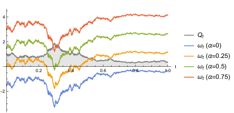
Fig. 1. Supply vs. Price for the values $\alpha=0$, $\alpha=0.1$, $\alpha=0.25$, $\alpha=0.5$

For a fixed simulation of the supply, we compute the price for different values of $\alpha$. Agents begin with zero energy average. The results are displayed in Figure 1. As expected, the price is negatively correlated with the supply. Moreover, as the storage target increases, prices increase, which reflects the competition between agents who, on average, want to increase their storage.

References

- [1] M. Burger, L. A. Caffarelli, P. A. Markowich, and Marie-Therese Wolfram. On a Boltzmann-type price formation model. Proc. R. Soc. Lond. Ser. A Math. Phys. Eng. Sci., 469(2157):20130126, 20, 2013.
- [2] L. A. Caffarelli, P. A. Markowich, and J.-F. Pietschmann. On a price formation free boundary model by Lasry and Lions. C. R. Math. Acad. Sci. Paris, 349(11-12):621–624, 2011.
- [3] René Carmona and Francois Delarue. The master equation for large population equilibriums. 2014.
- [4] René Carmona, François Delarue, and Daniel Lacker. Mean field games with common noise. Ann. Probab., 44(6):3740–3803, 11 2016.
- [5] A. Clemence, B. Tahar Imen, and M. Anis. An Extended Mean Field Game for Storage in Smart Grids. ArXiv e-prints, October 2017.
- [6] R. Couillet, S.M. Perlaza, H. Tembine, and M. Debbah. Electrical vehicles in the smart grid: A mean field game analysis. IEEE Journal on Selected Areas in Communications, 30(6):1086–1096, 2012. cited By 56.
- [7] A. De Paola, D. Angeli, and G. Strbac. Distributed control of micro-storage devices with mean field games. IEEE Transactions on Smart Grid, 7(2):1119–1127, 2016.
- [8] A. De Paola, V. Trovato, and D. Angeli. A mean field game approach for distributed control of thermostatic loads acting in simultaneous energy-frequency response markets. IEEE Transactions on Smart Grid, 2019.
- [9] D. Gomes, L. Lafleche, and L. Nurbekyan. A mean-field game economic growth model. Proceedings of the American Control Conference, 2016-July:4693–4698, 2016.
- [10] D. Gomes and J. Saúde. A mean-field game approach to price formation. To appear in Dynamic Games and Applications, 2019.
- [11] J. Graber and C. Mouzouni. Variational mean field games for market competition. arXiv e-prints, page arXiv:1707.07853, Jul 2017.
- [12] O. Guéant, J.-M. Lasry, and P.-L Lions. Mean field games and applications. In Paris-Princeton Lectures on Mathematical Finance 2010, volume 2003 of Lecture Notes in Math., pages 205–266. Springer, Berlin, 2011.
- [13] A.C. Kizilkale and R.P. Malhame. A class of collective target tracking problems in energy systems: Cooperative versus non-cooperative mean field control solutions. Proceedings of the IEEE Conference on Decision and Control, 2015-February(February):3493–3498, 2014.
- [14] A.C. Kizilkale and R.P. Malhame. Collective target tracking mean field control for electric space heaters. 2014 22nd Mediterranean Conference on Control and Automation, MED 2014, pages 829–834, 2014.
- [15] A.C. Kizilkale and R.P. Malhame. Collective target tracking mean field control for markovian jump-driven models of electric water heating loads. IFAC Proceedings Volumes (IFAC-PapersOnline), 19:1867–1872, 2014.
- [16] R. Malhamé and C.-Y. Chong. On the statistical properties of a cyclic diffusion process arising in the modeling of thermostat-controlled electric power system loads. SIAM J. Appl. Math., 48(2):465–480, 1988.
- [17] R. Malhamé, S. Kamoun, and D. Dochain. On-line identification of electric load models for load management. In Advances in computing and control (Baton Rouge, LA, 1988), volume 130 of Lect. Notes Control Inf. Sci., pages 290–304. Springer, Berlin, 1989.
- [18] P. A. Markowich, N. Matevosyan, J.-F. Pietschmann, and M.-T. Wolfram. On a parabolic free boundary equation modeling price formation. Math. Models Methods Appl. Sci., 19(10):1929–1957, 2009.