Hypergraph Motifs: Concepts, Algorithms, and Discoveries

Abstract

Hypergraphs naturally represent group interactions, which are omnipresent in many domains: collaborations of researchers, co-purchases of items, joint interactions of proteins, to name a few. In this work, we propose tools for answering the following questions in a systematic manner: (Q1) what are structural design principles of real-world hypergraphs? (Q2) how can we compare local structures of hypergraphs of different sizes? (Q3) how can we identify domains which hypergraphs are from? We first define hypergraph motifs (h-motifs), which describe the connectivity patterns of three connected hyperedges. Then, we define the significance of each h-motif in a hypergraph as its occurrences relative to those in properly randomized hypergraphs. Lastly, we define the characteristic profile (CP) as the vector of the normalized significance of every h-motif. Regarding Q1, we find that h-motifs’ occurrences in $11$ real-world hypergraphs from $5$ domains are clearly distinguished from those of randomized hypergraphs. In addition, we demonstrate that CPs capture local structural patterns unique to each domain, and thus comparing CPs of hypergraphs addresses Q2 and Q3. Our algorithmic contribution is to propose MoCHy, a family of parallel algorithms for counting h-motifs’ occurrences in a hypergraph. We theoretically analyze their speed and accuracy, and we show empirically that the advanced approximate version MoCHy-A⁺ is up to $25\times$ more accurate and $32\times$ faster than the basic approximate and exact versions, respectively.

1 Introduction

Complex systems consisting of pairwise interactions between individuals or objects are naturally expressed in the form of graphs. Nodes and edges, which compose a graph, represent individuals (or objects) and their pairwise interactions, respectively. Thanks to their powerful expressiveness, graphs have been used in a wide variety of fields, including social network analysis, web, bioinformatics, and epidemiology. Global structural patterns of real-world graphs, such as power-law degree distribution [10, 24] and six degrees of separation [33, 66], have been extensively investigated.

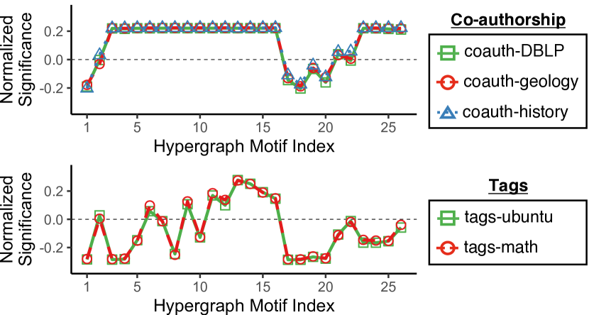
Figure 1: Distributions of h-motifs’ instances precisely characterize local structural patterns of real-world hypergraphs. Note that the hypergraphs from the same domains have similar distributions, while the hypergraphs from different domains do not. See Section 4.3 for details.

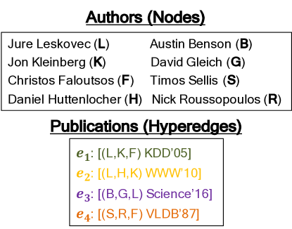
(a) Example data: coauthorship relations

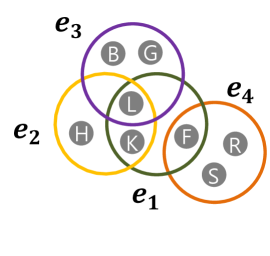
(b) Hypergraph representation

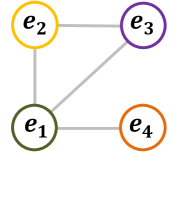
(c) Projected graph

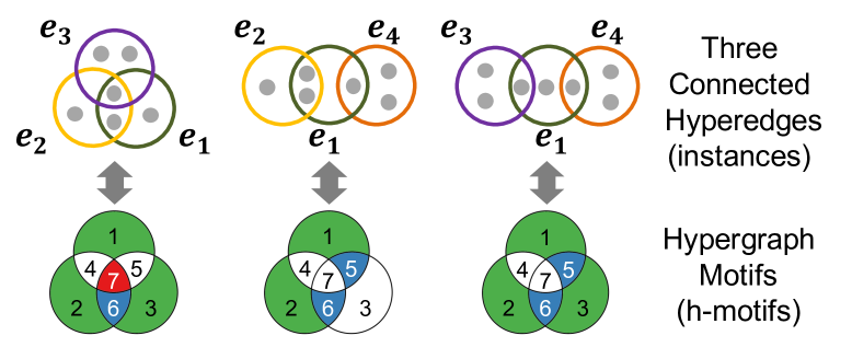
(d) H-motifs and instances

Figure 2: (a) Example: co-authorship relations. (b) Hypergraph: the hypergraph representation of (a). (c) Projected Graph: the projected graph of (b). (d) Hypergraph Motifs: example h-motifs and their instances in (b).

In addition to global patterns, real-world graphs exhibit patterns in their local structures, which differentiate graphs in the same domain from random graphs or those in other domains. Local structures are revealed by counting the occurrences of different network motifs [45, 46], which describe the patterns of pairwise interactions between a fixed number of connected nodes (typically $3$, $4$, or $5$ nodes). As a fundamental building block, network motifs have played a key role in many analytical and predictive tasks, including community detection [13, 43, 62, 68], classification [20, 39, 45], and anomaly detection [11, 57].

Despite the prevalence of graphs, interactions in many complex systems are groupwise rather than pairwise: collaborations of researchers, co-purchases of items, joint interactions of proteins, tags attached to the same web post, to name a few. These group interactions cannot be represented by edges in a graph. Suppose three or more researchers coauthor a publication. This co-authorship cannot be represented as a single edge, and creating edges between all pairs of the researchers cannot be distinguished from multiple papers coauthored by subsets of the researchers.

This inherent limitation of graphs is addressed by hypergraphs, which consist of nodes and hyperedges. Each hyperedge is a subset of any number of nodes, and it represents a group interaction among the nodes. For example, the coauthorship relations in Figure 2(a) are naturally represented as the hypergraph in Figure 2(b). In the hypergraph, seminar work [40] coauthored by Jure Leskovec (L), Jon Kleinberg (K), and Christos Faloutsos (F) is expressed as the hyperedge $e_{1}=\{L,K,F\}$, and it is distinguished from three papers coauthored by each pair, which, if they exist, can be represented as three hyperedges $\{K,L\}$, $\{F,L\}$, and $\{F,K\}$.

Table 1: Frequently-used symbols.

Notation	Definition
$G=(V,E)$	hypergraph with nodes $V$ and hyperedges $E$
$E=\{e_{1},...,e_{|E|}\}$	set of hyperedges
$E_{v}$	set of hyperedges that contains a node $v$
$\wedge$	set of hyperwedges in $G$
$\wedge_{ij}$	hyperwedge consisting of $e_{i}$ and $e_{j}$
$\bar{G}=(E,\wedge,\omega)$	projected graph of $G$
$\omega(\wedge_{ij})$	the number of nodes shared between $e_{i}$ and $e_{j}$
$N_{e_{i}}$	set of neighbors of $e_{i}$ in $\bar{G}$
$h(\{e_{i},e_{j},e_{k}\})$	h-motif corresponding to an instance $\{e_{i},e_{j},e_{k}\}$
$M[t]$	count of h-motif $t$’s instances

The successful investigation and discovery of local structural patterns in real-world graphs motivate us to explore local structural patterns in real-world hypergraphs. However, network motifs, which proved to be useful for graphs, are not trivially extended to hypergraphs. Due to the flexibility in the size of hyperedges, there can be infinitely many patterns of interactions among a fixed number of nodes, and other nodes can also be associated with these interactions.

In this work, taking these challenges into consideration, we define $26$ hypergraph motifs (h-motifs) so that they describe connectivity patterns of three connected hyperedges (rather than nodes). As seen in Figure 2(d), h-motifs describe the connectivity pattern of hyperedges $e_{1}$, $e_{2}$, and $e_{3}$ by the emptiness of seven subsets: $e_{1}\setminus e_{2}\setminus e_{3}$, $e_{2}\setminus e_{3}\setminus e_{1}$, $e_{3}\setminus e_{1}\setminus e_{2}$, $e_{1}\cap e_{2}\setminus e_{3}$, $e_{2}\cap e_{3}\setminus e_{1}$, $e_{3}\cap e_{1}\setminus e_{2}$, and $e_{1}\cap e_{2}\cap e_{3}$. As a result, every connectivity pattern is described by a unique h-motif, independently of the sizes of hyperedges. While this work focuses on connectivity patterns of three hyperedges, h-motifs are easily extended to four or more hyperedges.

We count the number of each h-motif’s instances in $11$ real-world hypergraphs from $5$ different domains. Then, we measure the significance of each h-motif in each hypergraph by comparing the count of its instances in the hypergraph against the counts in properly randomized hypergraphs. Lastly, we compute the characteristic profile (CP) of each hypergraph, defined as the vector of the normalized significance of every h-motif. Comparing the counts and CPs of different hypergraphs leads to the following observations:

• Structural design principles of real-world hypergraphs that are captured by frequencies of different h-motifs are clearly distinguished from those of randomized hypergraphs.

• Hypergraphs from the same domains have similar CPs, while hypergraphs from different domains have distinct CPs (see Figure 1). In other words, CPs successfully capture local structure patterns unique to each domain.

Our algorithmic contribution is to design MoCHy (Motif Counting in Hypergraphs), a family of parallel algorithms for counting h-motifs’ instances, which is the computational bottleneck of the aforementioned process. Note that since non-pairwise interactions are taken into consideration, counting the instances of h-motifs is more challenging than counting the instances of network motifs, which are defined solely based on pairwise interactions. We provide one exact version, named MoCHy-E, and two approximate versions, named MoCHy-A and MoCHy-A⁺. Empirically, MoCHy-A⁺ is up to $25\times$ more accurate than MoCHy-A, and it is up to $32\times$ faster than MoCHy-E, with little sacrifice of accuracy. These empirical results are consistent with our theoretical analyses.

In summary, our contributions are summarized as follow:

• Novel Concepts: We propose h-motifs, the counts of whose instances capture local structures of hypergraphs, independently of the sizes of hyperedges or hypergraphs.

• Fast and Provable Algorithms: We develop MoCHy, a family of parallel algorithms for counting h-motifs’ instances. We show theoretically and empirically that the advanced version significantly outperforms the basic ones, providing a better trade-off between speed and accuracy.

• Discoveries in $11$ Real-world Hypergraphs: We show that h-motifs and CPs reveal local structural patterns that are shared by hypergraphs from the same domains but distinguished from those of random hypergraphs and hypergraphs from other domains (see Figure 1).

Reproducibility: The code and datasets used in this work are available at https://github.com/geonlee0325/MoCHy.

In Section 2, we introduce h-motifs and characteristic profiles. In Section 3, we present exact and approximate algorithms for counting instances of h-motifs, and we analyze their theoretical properties. In Section 4, we provide experimental results. After discussing related work in Section 5, we offer conclusions in Section 6.

2 Proposed Concepts

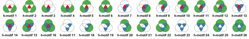
Figure 3: The 26 h-motifs studied in this work. Note that h-motifs 17 - 22 are open, while the others are closed.

In this section, we introduce the proposed concepts: hypergraph motifs and characteristic profiles. Refer Table 1 for the notations frequently used throughout the paper.

2.1 Preliminaries and Notations

We define some preliminary concepts and their notations.

Hypergraph Consider a hypergraph $G=(V,E)$, where $V$ and $E:=\{e_{1},e_{2},...,e_{|E|}\}$ are sets of nodes and hyperedges, respectively. Each hyperedge $e_{i}\in E$ is a non-empty subset of $V$, and we use $|e_{i}|$ to denote the number of nodes in it. For each node $v\in V$, we use $E_{v}:=\{e_{i}\in E:v\in e_{i}\}$ to denote the set of hyperedges that include $v$. We say two hyperedges $e_{i}$ and $e_{j}$ are adjacent if they share any member, i.e., if $e_{i}\cap e_{j}\neq\varnothing$. Then, for each hyperedge $e_{i}$, we denote the set of hyperedges adjacent to $e_{i}$ by $N_{e_{i}}:=\{e_{j}\in E:e_{i}\cap e_{j}\neq\varnothing\}$ and the number of such hyperedges by $|N_{e_{i}}|$. Similarly, we say three hyperedges $e_{i}$, $e_{j}$, and $e_{k}$ are connected if one of them is adjacent to two the others.

Hyperwedges: We define a hyperwedge as an unordered pair of adjacent hyperedges. We denote the set of hyperwedges in $G$ by $\wedge:=\{\{e_{i},e_{j}\}\in{E\choose 2}:e_{i}\cap e_{j}\neq\varnothing\}$. We use $\wedge_{ij}\in\wedge$ to denote the hyperwedge consisting of $e_{i}$ and $e_{j}$. In the example hypergraph in Figure 2(b), there are four hyperwedges: $\wedge_{12}$, $\wedge_{13}$, $\wedge_{23}$, and $\wedge_{14}$.

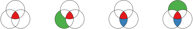
Figure 4: The h-motifs whose instances contain duplicated hyperedges.

Projected Graph: We define the projected graph of $G=(V,E)$ as $\bar{G}=(E,\wedge,\omega)$ where $\wedge$ is the set of hyperwedges and $\omega(\wedge_{ij}):=|e_{i}\cap e_{j}|$. That is, in the projected graph $\bar{G}$, hyperedges in $G$ act as nodes, and two of them are adjacent if and only if they share any member. Note that for each hyperedge $e_{i}\in E$, $N_{e_{i}}$ is the set of neighbors of $e_{i}$ in $\bar{G}$, and $|N_{e_{i}}|$ is its degree in $\bar{G}$. Figure 2(c) shows the projected graph of the example hypergraph in Figure 2(b).

2.2 Hypergraph Motifs

We introduce hypergraph motifs, which are basic building blocks of hypergraphs, with related concepts. Then, we discuss their properties and generalization.

Definition and Representation: Hypergraph motifs (or h-motifs in short) are for describing the connectivity patterns of three connected hyperedges. Specifically, given a set $\{e_{i},e_{j},e_{k}\}$ of three connected hyperedges, h-motifs describe its connectivity pattern by the emptiness of the following seven sets: (1) $e_{i}\setminus e_{j}\setminus e_{k}$, (2) $e_{j}\setminus e_{k}\setminus e_{i}$, (3) $e_{k}\setminus e_{i}\setminus e_{j}$, (4) $e_{i}\cap e_{j}\setminus e_{k}$, (5) $e_{j}\cap e_{k}\setminus e_{i}$, (6) $e_{k}\cap e_{i}\setminus e_{j}$, and (7) $e_{i}\cap e_{j}\cap e_{k}$. Formally, a h-motif is defined as a binary vector of size $7$ whose elements represent the emptiness of the above sets, respectively, and as seen in Figure 2(d), h-motifs are naturally represented in the Venn diagram. While there can be $2^{7}$ h-motifs, $26$ h-motifs remain once we exclude symmetric ones, those with duplicated hyperedges (see Figure 4), and those cannot be obtained from connected hyperedges. The 26 cases, which we call h-motif 1 through h-motif 26, are visualized in the Venn diagram in Figure 3.

Instances, Open h-motifs, and Closed h-motifs: Consider a hypergraph $G=(V,E)$. A set of three connected hyperedges is an instance of h-motif $t$ if their connectivity pattern corresponds to h-motif $t$. The count of each h-motif’s instances is used to characterize the local structure of $G$, as discussed in the following sections. A h-motif is closed if all three hyperedges in its instances are adjacent to (i.e., overlapped with) each other. If its instances contain two non-adjacent (i.e., disjoint) hyperedges, a h-motif is open. In Figure 3, h-motifs $17$ - $22$ are open; the others are closed.

Properties of h-motifs: From the definition of h-motifs, the following desirable properties are immediate:

• Exhaustive: h-motifs capture connectivity patterns of all possible three connected hyperedges.

• Unique: connectivity pattern of any three connected hyperedges is captured by at most one h-motif.

• Size Independent: h-motifs capture connectivity patterns independently of the sizes of hyperedges. Note that there can be infinitely many combinations of sizes of three connected hyperedges.

Note that the exhaustiveness and the uniqueness imply that connectivity pattern of any three connected hyperedges is captured by exactly one h-motif.

Why Non-pairwise Relations?: Non-pairwise relations
(e.g., the emptiness of $e_{1}\cap e_{2}\cap e_{3}$ and $e_{1}\setminus e_{2}\setminus e_{3}$) play a key role in capturing the local structural patterns of real-world hypergraphs. Taking only the pairwise relations (e.g., the emptiness of $e_{1}\cap e_{2}$, $e_{1}\setminus e_{2}$, and $e_{2}\setminus e_{1}$) into account limits the number of possible connectivity patterns of three distinct hyperedges to just eight, significantly limiting their expressiveness and thus usefulness. Specifically, $12$ (out of $26$) h-motifs have the same pairwise relations, while their occurrences and significances vary substantially in real-world hypergraphs. For example, in Figure 2, $\{e_{1},e_{2},e_{4}\}$ and $\{e_{1},e_{3},e_{4}\}$ have the same pairwise relations, while their connectivity patterns are distinguished by h-motifs.

Generalization to More than $3$ Hyperedges: The concept of h-motifs is easily generalized to four or more hyperedges. For example, a h-motif for four hyperedges can be defined as a binary vector of size $15$ indicating the emptiness of each region in the Venn diagram for four sets. After excluding disconnected ones, symmetric ones, and those with duplicated hyperedges, there remain $1,853$ and $18,656,322$ h-motifs for four and five hyperedges, respectively, as discussed in detail in Appendix F of [1]. This work focuses on the h-motifs for three hyperedges, which are already capable of characterizing local structures of real-world hypergraphs, as shown empirically in Section 4.

2.3 Characteristic Profile (CP)

What are the structural design principles of real-world hypergraphs distinguished from those of random hypergraphs? Below, we introduce the characteristic profile (CP), which is a tool for answering the above question using h-motifs.

Randomized Hypergraphs: While one might try to characterize the local structure of a hypergraph by absolute counts of each h-motif’s instances in it, some h-motifs may naturally have many instances. Thus, for more accurate characterization, we need random hypergraphs to be compared against real-world hypergraphs. We obtain such random hypergraphs by randomizing the compared real-world hypergraph. To this end, we represent the hypergraph $G=(V,E)$ as the bipartite graph $G^{\prime}$ where $V$ and $E$ are the two subsets of nodes, and there exists an edge between $v\in V$ and $e\in E$ if and only if $v\in e$ That is, $G^{\prime}=(V^{\prime},E^{\prime})$ where $V^{\prime}:=V\cup E$ and $E^{\prime}:=\{(v,e)\in V\times E:v\in e\}$. Then, we use the Chung-Lu model to generate bipartite graphs where the degree distribution of $G^{\prime}$ is well preserved [6]. Reversely, from each of the generated bipartite graphs, we can obtain a randomized hypergraph where the degree (i.e., the number of hyperedges that each node belongs to) distribution of nodes and the size distribution of hyperedges in $G$ are well preserved. We provide the pseudocode and the distributions in the randomized hypergraphs in Appendix D of [1].

Significance of H-motifs: We measure the significance of each h-motif in a hypergraph by comparing the count of its instances against the count of them in randomized hypergraphs. Specifically, the significance of a h-motif $t$ in a hypergraph $G$ is defined as

$$\Delta_{t}:=\frac{M[t]-M_{rand}[t]}{M[t]+M_{rand}[t]+\epsilon},\vspace{-1mm}$$ (1)

where $M[t]$ is the number of instances of h-motif $t$ in $G$, and $M_{rand}[t]$ is the average number of instances of h-motif $t$ in randomized hypergraphs. We fixed $\epsilon$ to $1$ throughout this paper. This way of measuring significance was proposed for network motifs as an alternative of normalized Z scores, which heavily depend on the graph size [45].

Characteristic Profile (CP): By normalizing and concatenating the significances of all h-motifs in a hypergraph, we obtain the characteristic profile (CP), which summarizes the local structural pattern of the hypergraph. Specifically, the characteristic profile of a hypergraph $G$ is a vector of size $26$, where each $t$-th element is

$$CP_{t}:=\frac{\Delta_{t}}{\sqrt{\sum_{t=1}^{26}\Delta_{t}^{2}}}.\vspace{-1mm}$$ (2)

Note that, for each $t$, $CP_{t}$ is between $-1$ and $1$. The CP is used in Section 4.3 to compare the local structural patterns of real-world hypergraphs from diverse domains.

3 Proposed Algorithms

Given a hypergraph, how can we count the instances of each h-motif? Once we count them in the original and randomized hypergraphs, the significance of each h-motif and the CP are obtained immediately by Eq. (1) and Eq. (2).

In this section, we present MoCHy (Motif Counting in Hypergraphs), which is a family of parallel algorithms for counting the instances of each h-motif in the input hypergraph. We first describe hypergraph projection, which is a preprocessing step of every version of MoCHy. Then, we present MoCHy-E, which is for exact counting. After that, we present two different versions of MoCHy-A, which are sampling-based algorithms for approximate counting. Lastly, we discuss parallel and on-the-fly implementations.

Throughout this section, we use $h(\{e_{i},e_{j},e_{k}\})$ to denote the h-motif that describes the connectivity pattern of an h-motif instance $\{e_{i},e_{j},e_{k}\}$. We also use $M[t]$ to denote the count of instances of h-motif $t$.

Input : input hypergraph: $G=(V,E)$

Output : projected graph: $\bar{G}=(E,\wedge,\omega)$

$\wedge\leftarrow\varnothing$

1 $\omega\leftarrow$ map whose default value is $0$

2 for each hyperedge $e_{i}\in E$  do

3       for each node $v\in e_{i}$  do

4             for each hyperedge $e_{j}\in E_{v}$ where $j>i$  do

5                   $\wedge\leftarrow\wedge\cup\{\wedge_{ij}\}$

6                   $\omega(\wedge_{ij})=\omega(\wedge_{ij})+1$

return $\bar{G}=(E,\wedge,\omega)$

Algorithm 1 Hypergraph Projection (Preprocess)

Remarks: The problem of counting h-motifs’ occurrences bears some similarity to the classic problem of counting network motifs’ occurrences. However, different from network motifs, which are defined solely based on pairwise interactions, h-motifs are defined based on triple-wise interactions (e.g., $e_{i}\cap e_{j}\cap e_{k}$). One might hypothesize that our problem can easily be reduced to the problem of counting the occurrences of network motifs, and thus existing solutions (e.g., [18, 50]) are applicable to our problem. In order to examine this possibility, we consider the following two attempts:

1. Represent pairwise relations between hyperedges using the projected graph, where each edge $\{e_{i},e_{j}\}$ indicates $e_{i}\cap e_{j}\neq\emptyset$.

2. Represent pairwise relations between hyperedges using the directed projected graph where each directed edge $e_{i}\rightarrow e_{j}$ indicates $e_{i}\cap e_{j}\neq\emptyset$ and at the same time $e_{i}\not\subset e_{j}$.

The number of possible connectivity patterns (i.e., network motifs) among three distinct connected hyperedges is just two (i.e., closed and open triangles) and eight in (a) and (b), respectively. In both cases, instances of multiple h-motifs are not distinguished by network motifs, and the occurrences of h-motifs can not be inferred from those of network motifs.

In addition, another computational challenge stems from the fact that triple-wise and even pair-wise relations between hyperedges need to be computed from the input hypergraph, while pairwise relations between edges are given in graphs. This challenge necessitates the precomputation of partial relations, described in the next subsection.

3.1 Hypergraph Projection (Algorithm 1)

As a preprocessing step, every version of MoCHy builds the projected graph $\bar{G}=(E,\wedge,\omega)$ (see Section 2.1) of the input hypergraph $G=(V,E)$, as described in Algorithm 1. To find the neighbors of each hyperedge $e_{i}$ (line 1), the algorithm visits each hyperedge $e_{j}$ that contains $v$ and satisfies $j>i$ (line 1) for each node $v\in e_{i}$ (line 1). Then for each such $e_{j}$, it adds $\wedge_{ij}=\{e_{i},e_{j}\}$ to $\wedge$ and increments $\omega(\wedge_{ij})$ (lines 1 and 1). The time complexity of this preprocessing step is given in Lemma 1.

Lemma 1 (Complexity of Hypergraph Projection).

The time complexity of Algorithm 1 is $O(\sum_{\wedge_{ij}\in\wedge}|e_{i}\cap e_{j}|)$.

Proof.

If all sets and maps are implemented using hash tables, lines 1 and 1 take $O(1)$ time, and they are executed $|e_{i}\cap e_{j}|$ times for each $\wedge_{ij}\in\wedge$. ∎

Since $|\wedge|<\sum_{e_{i}\in E}|{N}_{e_{i}}|$ and $|e_{i}\cap e_{j}|\leq|e_{i}|$, Eq. (3) holds.

$$\sum\nolimits_{\wedge_{ij}\in\wedge}|e_{i}\cap e_{j}|<\sum\nolimits_{e_{i}\in E}(|e_{i}|\cdot|N_{e_{i}}|).\vspace{-1mm}$$ (3)

Input :    (1) input hypergraph: $G=(V,E)$

(2) projected graph: $\bar{G}=(E,\wedge,\omega)$

Output : exact count of each h-motif $t$’s instances: $M[t]$

$M\leftarrow$ map whose default value is $0$

1 for each hyperedge $e_{i}\in E$  do

2       for each unordered hyperedge pair $\{e_{j},e_{k}\}\in$ $N_{e_{i}}\choose 2$ do

3             if $e_{j}\cap e_{k}=\varnothing$ or $i<\min(j,k)$ then

4                   $M[h(\{e_{i},e_{j},e_{k}\})]\mathrel{+}=1$

return $M$

Algorithm 2 MoCHy-E: Exact H-motif Counting

3.2 Exact H-motif Counting (Algorithm 2)

We present MoCHy-E (MoCHy Exact), which counts the instances of each h-motif exactly. The procedures of MoCHy-E are described in Algorithm 2. For each hyperedge $e_{i}\in E$ (line 2), each unordered pair $\{e_{j},e_{k}\}$ of its neighbors, where $\{e_{i},e_{j},e_{k}\}$ is an h-motif instance, is considered (line 2). If $e_{j}\cap e_{k}=\varnothing$ (i.e., if the corresponding h-motif is open), $\{e_{i},e_{j},e_{k}\}$ is considered only once. However, if $e_{j}\cap e_{k}\neq\varnothing$ (i.e., if the corresponding h-motif is closed), $\{e_{i},e_{j},e_{k}\}$ is considered two more times (i.e., when $e_{j}$ is chosen in line 2 and when $e_{k}$ is chosen in line 2). Based on these observations, given an h-motif instance $\{e_{i},e_{j},e_{k}\}$, the corresponding count $M[h(\{e_{i},e_{j},e_{k}\})]$ is incremented (line 2) only if $e_{j}\cap e_{k}=\varnothing$ or $i<\min(j,k)$ (line 2). This guarantees that each instance is counted exactly once. The time complexity of MoCHy-E is given in Theorem 1, which uses Lemma 2.

Lemma 2 (Time Complexity of Computing $h(\{e_{i},e_{j},e_{k}\})$).

Given the input hypergraph $G=(V,E)$ and its projected graph $\bar{G}=(E,\wedge,\omega)$, for each h-motif instance $\{e_{i},e_{j},e_{k}\}$, computing $h(\{e_{i},e_{j},e_{k}\})$ takes $O(\min(|e_{i}|,|e_{j}|,|e_{k}|))$ time.

Proof.

Assume $|e_{i}|=\min(|e_{i}|,|e_{j}|,|e_{k}|)$, without loss of generality, and all sets and maps are implemented using hash tables. As defined in Section 2.2, $h(\{e_{i},e_{j},e_{k}\})$ is computed in $O(1)$ time from the emptiness of the following sets: (1) $e_{i}\setminus e_{j}\setminus e_{k}$, (2) $e_{j}\setminus e_{k}\setminus e_{i}$, (3) $e_{k}\setminus e_{i}\setminus e_{j}$, (4) $e_{i}\cap e_{j}\setminus e_{k}$, (5) $e_{j}\cap e_{k}\setminus e_{i}$, (6) $e_{k}\cap e_{i}\setminus e_{j}$, and (7) $e_{i}\cap e_{j}\cap e_{k}$. We check their emptiness from their cardinalities. We obtain $e_{i}$, $e_{j}$, and $e_{k}$, which are stored in $G$, and their cardinalities in $O(1)$ time. Similarly, we obtain $|e_{i}\cap e_{j}|$, $|e_{j}\cap e_{k}|$, and $|e_{k}\cap e_{i}|$, which are stored in $\bar{G}$, in $O(1)$ time. Then, we compute $|e_{i}\cap e_{j}\cap e_{k}|$ in $O(|e_{i}|)$ time by checking for each node in $e_{i}$ whether it is also in both $e_{j}$ and $e_{k}$. From these cardinalities, we obtain the cardinalities of the six other sets in $O(1)$ time as follows:

$$(1)\ |e_{i}\setminus e_{j}\setminus e_{k}|=|e_{i}|-|e_{i}\cap e_{j}|-|e_{k}\cap e_{i}|+|e_{i}\cap e_{j}\cap e_{k}|,$$

$$(2)\ |e_{j}\setminus e_{k}\setminus e_{i}|=|e_{j}|-|e_{i}\cap e_{j}|-|e_{j}\cap e_{k}|+|e_{i}\cap e_{j}\cap e_{k}|,$$

$$(3)\ |e_{k}\setminus e_{i}\setminus e_{j}|=|e_{k}|-|e_{k}\cap e_{i}|-|e_{j}\cap e_{k}|+|e_{i}\cap e_{j}\cap e_{k}|,$$

$$(4)\ |e_{i}\cap e_{j}\setminus e_{k}|=|e_{i}\cap e_{j}|-|e_{i}\cap e_{j}\cap e_{k}|,$$

$$(5)\ |e_{j}\cap e_{k}\setminus e_{i}|=|e_{j}\cap e_{k}|-|e_{i}\cap e_{j}\cap e_{k}|,$$

$$(6)\ |e_{k}\cap e_{i}\setminus e_{j}|=|e_{k}\cap e_{i}|-|e_{i}\cap e_{j}\cap e_{k}|.$$

Hence, the time complexity of computing $h(\{e_{i},e_{j},e_{k}\})$ is $O(|e_{i}|)=O(\min(|e_{i}|,|e_{j}|,|e_{k}|))$. ∎

Theorem 1 (Complexity of MoCHy-E).

The time complexity of Algorithm 2 is $O(\sum_{e_{i}\in E}(|N_{e_{i}}|^{2}\cdot|e_{i}|))$.

Proof.

Assume all sets and maps are implemented using hash tables. The total number of triples $\{e_{i},e_{j},e_{k}\}$ considered in line 2 is $O(\sum_{e_{i}\in E}|N_{e_{i}}|^{2})$. By Lemma 2, for such a triple $\{e_{i},e_{j},e_{k}\}$, computing $h(\{e_{i},e_{j},e_{k}\})$ takes $O(|e_{i}|)$ time. Thus, the total time complexity of Algorithm 2 is $O(\sum_{e_{i}\in E}(|e_{i}|\cdot|N_{e_{i}}|^{2}))$, which dominates that of the preprocessing step (see Lemma 1 and Eq. (3)). ∎

Extension of MoCHy-E to H-motif Enumeration:
Since MoCHy-E visits all h-motif instances to count them, it is extended to the problem of enumerating every h-motif instance (with its corresponding h-motif), as described in Algorithm 3. The time complexity remains the same.

Input :    (1) input hypergraph: $G=(V,E)$

(2) projected graph: $\bar{G}=(E,\wedge,\omega)$

Output : h-motif instances and their corresponding h-motifs

for each hyperedge $e_{i}\in E$  do

1       for each unordered hyperedge pair $\{e_{j},e_{k}\}\in$ $N_{e_{i}}\choose 2$ do

2             if $e_{j}\cap e_{k}=\varnothing$ or $i<\min(j,k)$ then

3                   write($e_{i}$, $e_{j}$, $e_{k}$, $h(\{e_{i},e_{j},e_{k}\})$)

Algorithm 3 MoCHy-E_ENUM for H-motif Enumeration

Input :    (1) input hypergraph: $G=(V,E)$

(2) projected graph: $\bar{G}=(E,\wedge,\omega)$

(3) number of samples: $s$

Output : estimated count of each h-motif $t$’s instances: $\bar{M}[t]$

$\bar{M}[t]\leftarrow$ map whose default value is $0$

1 for $n\leftarrow 1...s$ do

2       $e_{i}\leftarrow$ sample a uniformly random hyperedge

3       for each hyperedge $e_{j}\in N_{e_{i}}$ do

4             for each hyperedge $e_{k}\in(N_{e_{i}}\cup N_{e_{j}}\setminus\{e_{i},e_{j}\})$ do

5                   if $e_{k}\not\in N_{e_{i}}$ or $j<k$ then

6                         $\bar{M}[h(\{e_{i},e_{j},e_{k}\})]\mathrel{+}=1$

7 for each h-motif $t$ do

8       $\bar{M}[t]\leftarrow\bar{M}[t]\cdot\tfrac{|E|}{3s}$

return $\bar{M}$

Algorithm 4 MoCHy-A: Approximate H-motif Counting Based on Hyperedge Sampling

3.3 Approximate H-motif Counting

We present two different versions of MoCHy-A (MoCHy Approximate), which approximately count the instances of each h-motif. Both versions yield unbiased estimates of the counts by exploring the input hypergraph partially through hyperedge and hyperwedge sampling, respectively.

MoCHy-A: Hyperedge Sampling (Algorithm 4):

MoCHy-A (Algorithm 4) is based on hyperedge sampling. It repeatedly samples $s$ hyperedges from the hyperedge set $E$ uniformly at random with replacement (line 4). For each sampled hyperedge $e_{i}$, the algorithm searches for all h-motif instances that contain $e_{i}$ (lines 4-4), and to this end, the $1$-hop and $2$-hop neighbors of $e_{i}$ in the projected graph $\bar{G}$ are explored. After that, for each such instance $\{e_{i},e_{j},e_{k}\}$ of h-motif $t$, the corresponding count $\bar{M}[t]$ is incremented (line 4). Lastly, each estimate $\bar{M}[t]$ is rescaled by multiplying it with $\frac{|E|}{3s}$ (lines 4-4), which is the reciprocal of the expected number of times that each of the h-motif $t$’s instances is counted. This rescaling makes each estimate $\bar{M}[t]$ unbiased, as formalized in Theorem 2.

Theorem 2 (Bias and Variance of MoCHy-A).

For every h-motif t, Algorithm 4 provides an unbiased estimate $\bar{M}[t]$ of the count $M[t]$ of its instances, i.e.,

$$\mathbb{E}[\bar{M}[t]]=M[t].\vspace{-1mm}$$ (4)

The variance of the estimate is

$$\mathbb{V}\mathrm{ar}[\bar{M}[t]]=\frac{1}{3s}\cdot M[t]\cdot(|E|-3)+\frac{1}{9s}\sum_{l=0}^{2}p_{l}[t]\cdot(l|E|-9),\vspace{-1mm}$$ (5)

where $p_{l}[t]$ is the number of pairs of h-motif $t$’s instances that share $l$ hyperedges.

Proof.

See Appendix A. ∎

The time complexity of MoCHy-A is given in Theorem 3.

Theorem 3 (Complexity of MoCHy-A).

The average time complexity of Algorithm 4 is $O(\frac{s}{|E|}\sum_{e_{i}\in E}(|e_{i}|\cdot|N_{e_{i}}|^{2}))$.

Proof.

Assume all sets and maps are implemented using hash tables. For a sample hyperedge $e_{i}$, computing $N_{e_{i}}\cup N_{e_{j}}$ for every $e_{j}\in N_{e_{i}}$ takes $O(\sum_{e_{j}\in N_{e_{i}}}(|N_{e_{i}}\cup N_{e_{j}}|))$ time, and by Lemma 2, computing $h(\{e_{i},e_{j},e_{k}\})$ for all considered h-motif instances takes $O(\min(|e_{i}|,|e_{j}|)\cdot\sum_{e_{j}\in N_{e_{i}}}|N_{e_{i}}\cup N_{e_{j}}|)$ time. Thus, from $|N_{e_{i}}\cup N_{e_{j}}|\leq|N_{e_{i}}|+|N_{e_{j}}|$, the time complexity for processing a sample $e_{i}$ is

$$O(\min(|e_{i}|,|e_{j}|)\cdot\sum\nolimits_{e_{j}\in N_{e_{i}}}(|N_{e_{i}}|+|N_{e_{j}}|))\\ =O(|e_{i}|\cdot|N_{e_{i}}|^{2}+\sum\nolimits_{e_{j}\in N_{e_{i}}}(|e_{j}|\cdot|N_{e_{j}}|)),\vspace{-1mm}$$

which can be written as

$$O(\sum\nolimits_{e_{i}\in E}(\mathbb{1}(e_{i}\text{ is sampled})\cdot|e_{i}|\cdot|N_{e_{i}}|^{2})\\ +\sum\nolimits_{e_{j}\in E}(\mathbb{1}(e_{j}\text{ is adjacent to the sample})\cdot|e_{j}|\cdot|N_{e_{j}}|)).\vspace{-1mm}$$

From this, linearity of expectation, $\mathbb{E}[\mathbb{1}(e_{i}$ is sampled$)]=\frac{1}{|E|}$, and $\mathbb{E}[\mathbb{1}(e_{j}$ is adjacent to the sample$)]=\frac{|N_{e_{j}}|}{|E|}$, the average time complexity per sample hyperedge becomes $O(\frac{1}{|E|}$ $\sum_{e_{i}\in E}(|e_{i}|\cdot|N_{e_{i}}|^{2}))$. Hence, the total time complexity for processing $s$ samples is $O(\frac{s}{|E|}\sum_{e_{i}\in E}(|e_{i}|\cdot|N_{e_{i}}|^{2}))$.∎

Input :    (1) input hypergraph: $G=(V,E)$

(2) projected graph: $\bar{G}=(E,\wedge,\omega)$

(3) number of samples: $r$

Output : estimated count of each h-motif $t$’s instances: $\hat{M}[t]$

$\hat{M}\leftarrow$ map whose default value is $0$

1 for $n\leftarrow 1...r$ do

2       $\wedge_{ij}\leftarrow$ a uniformly random hyperwedge

3       for each hyperedge $e_{k}\in(N_{e_{i}}\cup N_{e_{j}}\setminus\{e_{i},e_{j}\})$ do

4             $\hat{M}[h(\{e_{i},e_{j},e_{k}\})]\mathrel{+}=1$

5      

6for each h-motif $t$ do

7       if 17 $\leq$ t $\leq$ 22 then $\triangleright$ open h-motifs

8             $\hat{M}[t]\leftarrow\hat{M}[t]\cdot\tfrac{|\wedge|}{2r}$

9      else $\triangleright$ closed h-motifs

10             $\hat{M}[t]\leftarrow\hat{M}[t]\cdot\tfrac{|\wedge|}{3r}$

return $\hat{M}$

Algorithm 5 MoCHy-A⁺: Approximate H-motif Counting Based on Hyperwedge Sampling

MoCHy-A⁺: Hyperwedge Sampling (Algorithm 5):

MoCHy-A⁺ (Algorithm 5) provides a better trade-off between speed and accuracy than MoCHy-A. Different from MoCHy-A, which samples hyperedges, MoCHy-A⁺ is based on hyperwedge sampling. It selects $r$ hyperwedges uniformly at random with replacement (line 5), and for each sampled hyperwedge $\wedge_{ij}\in\wedge$, it searches for all h-motif instances that contain $\wedge_{ij}$ (lines 5-5). To this end, the hyperedges that are adjacent to $e_{i}$ or $e_{j}$ in the projected graph $\bar{G}$ are considered (line 5). For each such instance $\{e_{i},e_{j},e_{k}\}$ of h-motif $t$, the corresponding estimate $\hat{M}[t]$ is incremented (line 5). Lastly, each estimate $\hat{M}[t]$ is rescaled so that it unbiasedly estimates $M[t]$, as formalized in Theorem 4. To this end, it is multiplied by the reciprocal of the expected number of times that each instance of h-motif $t$ is counted.

Theorem 4 (Bias and Variance of MoCHy-A⁺).

For every h-motif t, Algorithm 5 provides an unbiased estimate $\hat{M}[t]$ of the count $M[t]$ of its instances, i.e.,

$$\mathbb{E}[\hat{M}[t]]=M[t].\vspace{-1mm}$$ (6)

For every closed h-motif $t$, the variance of the estimate is

$$\mathbb{V}\mathrm{ar}[\hat{M}[t]]=\frac{1}{3r}\cdot M[t]\cdot(|\wedge|-3)+\frac{1}{9r}\sum_{n=0}^{1}q_{n}[t]\cdot(n|\wedge|-9),\vspace{-1mm}$$ (7)

where $q_{n}[t]$ is the number of pairs of h-motif $t$’s instances that share $n$ hyperwedges. For every open h-motif $t$, the variance is

$$\mathbb{V}\mathrm{ar}[\hat{M}[t]]=\frac{1}{2r}\cdot M[t]\cdot(|\wedge|-2)+\frac{1}{4r}\sum_{n=0}^{1}q_{n}[t]\cdot(n|\wedge|-4).\vspace{-2mm}$$ (8)

Proof.

See Appendix B. ∎

The time complexity of MoCHy-A⁺ is given in Theorem 5.

Theorem 5 (Complexity of MoCHy-A⁺).

The average time complexity of Algorithm 5 is $O(\frac{r}{|\wedge|}\sum_{e_{i}\in E}(|e_{i}|\cdot|N_{e_{i}}|^{2}))$.

Proof.

Assume all sets and maps are implemented using hash tables. For a sample hyperwedge $\wedge_{ij}$, computing $N_{e_{i}}\cup N_{e_{j}}$ takes $O(|N_{e_{i}}\cup N_{e_{j}}|)$ time, and by Lemma 2, computing $h(\{e_{i},e_{j},e_{k}\})$ for all considered h-motif instances takes $O(\min(|e_{i}|,|e_{j}|)\cdot|N_{e_{i}}\cup N_{e_{j}}|)$ time. Thus, from $|N_{e_{i}}\cup N_{e_{j}}|\leq|N_{e_{i}}|+|N_{e_{j}}|$, the time complexity for processing a sample $\wedge_{ij}$ is $O(\min(|e_{i}|,|e_{j}|)\cdot(|N_{e_{i}}|+|N_{e_{j}}|))=O(|e_{i}|\cdot|N_{e_{i}}|+|e_{j}|\cdot|N_{e_{j}}|),$ which can be written as

$$O(\sum\nolimits_{e_{i}\in E}(\mathbb{1}(e_{i}\text{ is included in the sample})\cdot|e_{i}|\cdot|N_{e_{i}}|)\\ +\sum\nolimits_{e_{j}\in E}(\mathbb{1}(e_{j}\text{ is included in the sample})\cdot|e_{j}|\cdot|N_{e_{j}}|)).\vspace{-1mm}$$

From this, linearity of expectation, $\mathbb{E}[\mathbb{1}(e_{i}$ is included in the sample$)]=\frac{|N_{e_{i}}|}{|\wedge|}$, and $\mathbb{E}[\mathbb{1}(e_{j}$ is included in the sample$)]=\frac{|N_{e_{j}}|}{|\wedge|}$, the average time complexity per sample hyperwedge is $O(\frac{1}{|\wedge|}\sum_{e_{i}\in E}(|e_{i}|\cdot|N_{e_{i}}|^{2}))$. Hence, the total time complexity for processing $r$ samples is $O(\frac{r}{|\wedge|}\sum_{e_{i}\in E}(|e_{i}|\cdot|N_{e_{i}}|^{2}))$.∎

Comparison of MoCHy-A and MoCHy-A⁺: Empirically, MoCHy-A⁺ provides a better trade-off between speed and accuracy than MoCHy-A, as presented in Section 4.5. We provide an analysis that supports this observation. Assume that the numbers of samples in both algorithms are set so that $\alpha=\frac{s}{|E|}=\frac{r}{|\wedge|}$. For each h-motif $t$, since both estimates $\bar{M}[t]$ of MoCHy-A and $\hat{M}[t]$ of MoCHy-A⁺ are unbiased (see Eqs. (4) and (6)), we only need to compare their variances. By Eq. (5), $\mathbb{V}\mathrm{ar}[\bar{M}[t]]=O(\frac{M[t]+p_{1}[t]+p_{2}[t]}{\alpha})$, and by Eq. (7) and Eq. (8), $\mathbb{V}\mathrm{ar}[\hat{M}[t]]=O(\frac{M[t]+q_{1}[t]}{\alpha})$. By definition, $q_{1}[t]\leq p_{2}[t]$, and thus $\frac{M[t]+q_{1}[t]}{\alpha}\leq\frac{M[t]+p_{1}[t]+p_{2}[t]}{\alpha}$. Moreover, in real-world hypergraphs, $p_{1}[t]$ tends to be several orders of magnitude larger than the other terms (i.e., $p_{2}[t]$, $q_{1}[t]$, and $M[t]$), and thus $\bar{M}[t]$ of MoCHy-A tends to have larger variance (and thus larger estimation error) than $\hat{M}[t]$ of MoCHy-A⁺. Despite this fact, as shown in Theorems 3 and 5, MoCHy-A and MoCHy-A⁺ have the same time complexity, $O(\alpha\cdot\sum_{e_{i}\in E}(|e_{i}|\cdot|N_{e_{i}}|^{2}))$. Hence, MoCHy-A⁺ is expected to give a better trade-off between speed and accuracy than MoCHy-A, as confirmed empirically in Section 4.5.

Table 2: Statistics of 11 real hypergraphs from 5 domains.

Dataset	$|V|$	$|E|$	$|\bar{e}|$*	$|\wedge|$	# H-motifs
coauth-DBLP	1,924,991	2,466,792	25	125M	26.3B $\pm$ 18M
coauth-geology	1,256,385	1,203,895	25	37.6M	6B $\pm$ 4.8M
coauth-history	1,014,734	895,439	25	1.7M	83.2M
contact-primary	242	12,704	5	2.2M	617M
contact-high	327	7,818	5	593K	69.7M
email-Enron	143	1,512	18	87.8K	9.6M
email-EU	998	25,027	25	8.3M	7B
tags-ubuntu	3,029	147,222	5	564M	4.3T $\pm$ 1.5B
tags-math	1,629	170,476	5	913M	9.2T $\pm$ 3.2B
threads-ubuntu	125,602	166,999	14	21.6M	11.4B
threads-math	176,445	595,749	21	647M	2.2T $\pm$ 883M
$*$ The maximum size of a hyperedge.

3.4 Parallel and On-the-fly Implementations

We discuss parallelization of MoCHy and then on-the-fly computation of projected graphs.

Parallelization: All versions of MoCHy and hypergraph projection are easily parallelized. Specifically, we can parallelize hypergraph projection and MoCHy-E by letting multiple threads process different hyperedges (in line 1 of Algorithm 1 and line 2 of Algorithm 2) independently in parallel. Similarly, we can parallelize MoCHy-A and MoCHy-A⁺ by letting multiple threads sample and process different hyperedges (in line 4 of Algorithm 4) and hyperwedges (in line 5 of Algorithm 5) independently in parallel. The estimated counts of the same h-motif obtained by different threads are summed up only once before they are returned as outputs. We present some empirical results in Section 4.5.

H-motif Counting without Projected Graphs: If the input hypergraph $G$ is large, computing its projected graph $\bar{G}$ (Algorithm 1) is time and space consuming. Specifically, building $\bar{G}$ takes $O(\sum_{\wedge_{ij}\in\wedge}|e_{i}\cap e_{j}|)$ time (see Lemma 1) and requires $O(|E|+|\wedge|)$ space, which often exceeds $O(\sum_{e_{i}\in E}$ $|e_{i}|)$ space required for storing $G$. Thus, instead of precomputing $\bar{G}$ entirely, we can build it incrementally while memoizing partial results within a given memory budget. For example, in MoCHy-A⁺ (Algorithm 5), we compute the neighborhood of a hyperedge $e_{i}\in E$ in $\bar{G}$ (i.e., $\{(k,\omega(\wedge_{ik})):k\in N_{e_{i}}\}$) only if (1) a hyperwedge with $e_{i}$ (e.g., $\wedge_{ij}$) is sampled (in line 5) and (2) its neighborhood is not memoized, as described in the pseudocode in Appendix G of [1]. Whether they are computed on the fly or read from memoized results, we always use exact neighborhoods, and thus this change does not affect the accuracy of the considered algorithm.

This incremental computation of $\bar{G}$ can be beneficial in terms of speed since it skips projecting the neighborhood of a hyperedge if no hyperwedge containing it is sampled. However, it can also be harmful if memoized results exceed the memory budget and some parts of $\bar{G}$ need to be rebuilt multiple times. Then, given a memory budget in bits, how should we prioritize hyperedges if all their neighborhoods cannot be memoized? According to our experiments, despite their large size, memoizing the neighborhoods of hyperedges with high degree in $\bar{G}$ makes MoCHy-A⁺ faster than memoizing the neighborhoods of randomly chosen hyperedges or least recently used (LRU) hyperedges. We experimentally examine the effects of the memory budget in Section 4.5.

4 Experiments

Table 3: Real-world and random hypergraphs have distinct distributions of h-motif instances. We report the absolute counts of each h-motif’s instances in a real-world hypergraph from each domain and its corresponding random hypergraph. To compare the counts in both hypergraphs, we measure the relative count (RC) of each h-motif. We also rank the counts, and we report each h-motif’s rank difference (RD) in the real-world and corresponding random hypergraphs.

In this section, we review our experiments that we design for answering the following questions:

• Q1. Comparison with Random: Does counting instances of different h-motifs reveal structural design principles of real-world hypergraphs distinguished from those of random hypergraphs?

• Q2. Comparison across Domains: Do characteristic profiles capture local structural patterns of hypergraphs unique to each domain?

• Q3. Observations and Applications: What are interesting discoveries and applications of h-motifs in real-world hypergraphs?

• Q4. Performance of Counting Algorithms: How fast and accurate are the different versions of MoCHy? Does the advanced version outperform the basic ones?

4.1 Experimental Settings

Machines: We conducted all the experiments on a machine with an AMD Ryzen 9 3900X CPU and 128GB RAM.

Implementations: We implemented all versions of MoCHy using C++ and OpenMP.

Datasets: We used the following eleven real-world hypergraphs from five different domains:

• co-authorship (coauth-DBLP, coauth-geology [58], and coauth-history [58]): A node represents an author. A hyperedge represents all authors of a publication.

• contact (contact-primary [59] and contact-high [44]): A node represents a person. A hyperedge represents a group interaction among individuals.

• email (email-Enron [37] and email-EU [40, 68]): A node represents an e-mail account. A hyperedge consists of the sender and all receivers of an email.

• tags (tags-ubuntu and tags-math): A node represents a tag. A hyperedge represents all tags attached to a post.

• threads (threads-ubuntu and threads-math): A node represents a user. A hyperedge groups all users participating in a thread.

These hypergraphs are made public by the authors of [12], and in Table 2 we provide some statistics of the hypergraphs after removing duplicated hyperedges. We used MoCHy-E for the coauth-history dataset, the threads-ubuntu dataset, and all datasets from the contact and email domains. For the other datasets, we used MoCHy-A⁺ with $r=2,000,000$, unless otherwise stated. We used a single thread unless otherwise stated. We computed CPs based on five hypergraphs randomized as described in Section 2.2.

4.2 Q1. Comparison with Random

We analyze the counts of different h-motifs’ instances in real and random hypergraphs. In Table 3, we report the (approximated) count of each h-motif $t$’s instances in each real hypergraph with the corresponding count averaged over five random hypergraphs obtained as described in Section 2.2. For each h-motif $t$, we measure its relative count, which we define as $\frac{M[t]-M_{rand}[t]}{M[t]+M_{rand}[t]}.$ We also rank h-motifs by the counts of their instances and examine the difference between the ranks in real and corresponding random hypergraphs. As seen in the table, the count distributions in real hypergraphs are clearly distinguished from those of random hypergraphs.

H-motifs in Random Hypergraphs: We notice that instances of h-motifs $17$ and $18$ appear much more frequently in random hypergraphs than in real hypergraphs from all domains. For example, instances of h-motif $17$ appear only about $510$ thousand times in the tags-math dataset, while they appear about $500$ million times (about $\mathbf{980\times}$ more often) in the corresponding randomized hypergraph. In the threads-math dataset, instances of h-motif $18$ appear about $830$ thousand times, while they appear about $13$ billion times (about $\mathbf{15,660\times}$ more often) in the corresponding randomized hypergraph. Instances of h-motifs $17$ and $18$ consist of a hyperedge and its two disjoint subsets (see Figure 3).

H-motifs in Co-authorship Hypergraphs: We observe that instances of h-motifs $10$, $11$ and $12$ appear more frequently in all three hypergraphs from the co-authorship domain than in the corresponding random hypergraphs. Although there are only about $190$ instances of h-motif $12$ in the corresponding random hypergraphs, there are about $64$ million such instances (about $\mathbf{337,000\times}$ more instances) in the coauth-DBLP dataset. As seen in Figure 3, in instances of h-motifs $10$, $11$, and $12$, a hyperedge is overlapped with the two other overlapped hyperedges in three different ways.

H-motifs in Contact Hypergraphs: Instances of h-motifs $9$, $13$, and $14$ are noticeably more common in both contact datasets than in the corresponding random hypergraphs. As seen in Figure 3, in instances of h-motifs $9$, $13$ and $14$, hyperedges are tightly connected and nodes are mainly located in the intersections of all or some hyperedges.

H-motifs in Email Hypergraphs: Both email datasets contain particularly many instances of h-motifs $8$ and $10$, compared to the corresponding random hypergraphs. As seen in Figure 3, instances of h-motifs $8$ and $10$ consist of three hyperedges one of which contains most nodes.

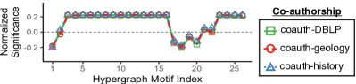
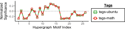
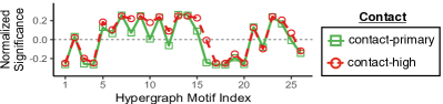
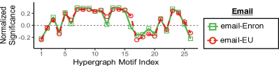
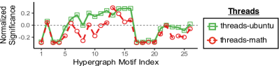
Figure 5: Characteristic profiles (CPs) capture local structural patterns of real-world hypergraphs accurately. The CPs are similar within domains but different across domains. Note that the significance of h-motif 3 distinguishes the contact hypergraphs from the email hypergraphs.

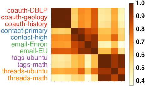
(a) Similarity matrix based on hypergraph motifs

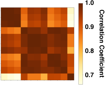
(b) Similarity matrix based on network motifs

Figure 6: Characteristic profiles (CPs) based on hypergraph motifs (h-motifs) capture local structural patterns more accurately than CPs based on network motifs. The CPs based on h-motifs distinguishes the domains of the real-world hypergraphs better than the CPs based on network motifs.

H-motifs in Tags Hypergraphs: In addition to instances of h-motif $11$, which are common in most real hypergraphs, instances of h-motif $16$, where all seven regions are not empty (see Figure 3), are particularly frequent in both tags datasets than in corresponding random hypergraphs.

H-motifs in Threads Hypergraphs: Lastly, in both data sets from the threads domain, instances of h-motifs $12$ and $24$ are noticeably more frequent than expected from the corresponding random hypergrpahs.

In Appendix C.1 of [1], we analyze how the significance of each h-motif and the rank difference for it are related to global structural properties of hypergraphs.

4.3 Q2. Comparison across Domains

We compare the characteristic profiles (CPs) of the real-world hypergraphs. In Figure 5, we present the CPs (i.e., the significances of the $26$ h-motifs) of each hypergraph. As seen in the figure, hypergraphs from the same domains have similar CPs. Specifically, all three hypergraphs from the co-authorship domain share extremely similar CPs, even when the absolute counts of h-motifs in them are several orders of magnitude different. Similarly, the CPs of both hypergraphs from the tags domain are extremely similar. However, the CPs of the three hypergraphs from the co-authorship domain are clearly distinguished by them of the hypergraphs from the tags domain. While the CPs of the hypergraphs from the contact domain and the CPs of those from the email domain are similar for the most part, they are distinguished by the significance of h-motif 3. These observations confirm that CPs accurately capture local structural patterns of real-world hypergraphs. In Appendix LABEL:appendix:addExp-motifSignificance of [1], we analyze the importance of each h-motif in terms its contribution to distinguishing the domains.

To further verify the effectiveness of CPs based on h-motifs, we compare them with CPs based on network motifs. Specifically, we represent each hypergraph $G=(V,E)$ as a bipartite graph $G^{\prime}=(V^{\prime},E^{\prime})$ where $V^{\prime}:=V\cup E$ and $E^{\prime}:=\{(v,e)\in V\times E:v\in e\}$, which is also known as star expansion [60]. That is, the two types of nodes in the transformed bipartite graph $G^{\prime}$ represent the nodes and hyperedges, respectively, in the original hypergraph $G$, and each edge $(v,e)$ in $G^{\prime}$ indicates that the node $v$ belongs to the hyperedge $e$ in $G$. Then, we compute the CPs based on the network motifs consisting of $3$ to $5$ nodes, using [18]. Lastly, based on both CPs, we compute the similarity matrices (specifically, correlation coefficient matrices) of the real-world hypergraphs. As seen in Figure 6, the domains of the real-world hypergraphs are distinguished more clearly by the CPs based on h-motifs than by the CPs based on network motifs. Numerically, when the CPs based on h-motifs are used, the average correlation coefficient is $0.978$ within domains and $0.654$ across domains, and the gap is $0.324$. However, when the CPs based on network motifs are used, the average correlation coefficient is $0.988$ within domains and $0.919$ across domains, and the gap is just $0.069$. These results support that h-motifs play a key role in capturing local structural patterns of real-world hypergraphs.

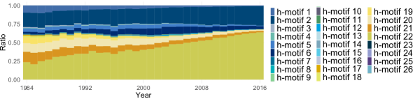
(a) Fraction of the instances of each h-motif in the coauth-DBLP dataset over time.

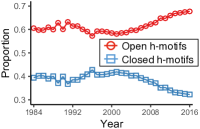
(b) Open and closed h-motifs.

Figure 7: Trends in the formation of collaborations are captured by h-motifs. (a) The fractions of the instances of h-motifs 2 and 22 have increased rapidly. (b) The fraction of the instances of open h-motifs has increased steadily since 2001.

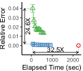
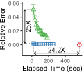
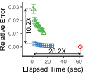
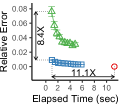
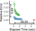
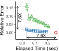
(a) threads-ubuntu

(b) email-Eu

(c) contact-primary

(d) coauth-history

(e) contact-high

(f) email-Enron

Figure 8: MoCHy-A⁺ gives the best trade-off between speed and accuracy. It yields up to $25\times$ more accurate estimation than MoCHy-A, and it is up to $32.5\times$ faster than MoCHy-E. The error bars indicate $\pm$ $1$ standard error over $20$ trials.

Table 4: H-motifs give informative features. Using them in HM26 or HM7 yields more accurate hyperedge predictions than using the baseline features in HC.

		HM26	HM7	HC
Logistic Regression	ACC$*$	0.754	0.656	0.636
	AUC$\dagger$	0.813	0.693	0.691
Random Forest	ACC	0.768	0.741	0.639
	AUC	0.852	0.779	0.692
Decision Tree	ACC	0.731	0.684	0.613
	AUC	0.732	0.685	0.616
K-Nearest Neighbors	ACC	0.694	0.689	0.640
	AUC	0.750	0.743	0.684
MLP Classifier	ACC	0.795	0.762	0.646
	AUC	0.875	0.841	0.701
$*$ acuracy, $\dagger$ area under the ROC curve.

4.4 Q3. Observations and Applications

We conduct two case studies on the coauth-DBLP dataset, which is a co-authorship hypergraph.

Evolution of Co-authorship Hypergraphs: The data-set contains bibliographic information of computer science publications. Using the publications in each year from $1984$ to $2016$, we create $33$ hypergraphs where each node corresponds to an author, and each hyperedge indicates the set of the authors of a publication. Then, we compute the fraction of the instances of each h-motif in each hypergraph to analyze patterns and trends in the formation of collaborations. As shown in Figure 7, over the 33 years, the fractions have changed with distinct trends. First, as seen in Figure 7(b), the fraction of the instances of open h-motifs has increased steadily since 2001, indicating that collaborations have become less clustered, i.e., the probability that two collaborations intersecting with a collaboration also intersect with each other has decreased. Notably, the fractions of the instances of h-motif $2$ (closed) and h-motif $22$ (open) have increased rapidly, accounting for most of the instances.

Hyperedge Prediction: As an application of h-motifs, we consider the problem of predicting publications (i.e., hyperedges) in $2016$ based on the publications from $2013$ to $2015$. As in [69], we formulate this problem as a binary classification problem where we aim to classify real hyperedges and fake ones. To this end, we create fake hyperedges in both training and test sets by replacing some fraction of nodes in each real hyperedge with random nodes (see Appendix E of [1] for details). Then, we train five classifiers using the following three different sets of input hyperedge features:

• HM26 ($\in\mathbb{R}^{26}$): The number of each h-motif’s instances that contain each hyperedge.

• HM7 ($\in\mathbb{R}^{7}$): The seven features with the largest variance among those in HM26.

• HC ($\in\mathbb{R}^{7}$): The mean, maximum, and minimum degree and the mean, maximum, and minimum number of neighbors of the nodes in each hyperedge and its size.

We report the accuracy (ACC) and the area under the ROC curve (AUC) in each setting in Table 4. Using HM7, which is based on h-motifs, yields consistently better predictions than using an equal number of baseline features in HC. Using HM26 yields the best predictions. These results indicate informative features can be obtained from h-motifs.

4.5 Q4. Performance of Counting Algorithms

We test the speed and accuracy of all versions of MoCHy under various settings. To this end, we measure elapsed time and relative error defined as

$$\frac{\sum_{t=1}^{26}|M[t]-\bar{M}[t]|}{\sum_{t=1}^{26}M[t]}\text{ and }\frac{\sum_{t=1}^{26}|M[t]-\hat{M}[t]|}{\sum_{t=1}^{26}M[t]},$$

for MoCHy-A and MoCHy-A⁺, respectively.

Speed and Accuracy: In Figure 8, we report the elapsed time and relative error of all versions of MoCHy on the $6$ different datasets where MoCHy-E terminates within a reasonable time. The numbers of samples in MoCHy-A and MoCHy-A⁺ are set to $\{2.5\times k:1\leq k\leq 10\}$ percent of the counts of hyperedges and hyperwedges, respectively. MoCHy-A⁺ provides the best trade-off between speed and accuracy. For example, in the threads-ubuntu dataset, MoCHy-A⁺ provides $24.6\times$ lower relative error than MoCHy-A, consistently with our theoretical analysis (see the last paragraph of Section 3.3). Moreover, in the same dataset, MoCHy-A⁺ is $32.5\times$ faster than MoCHy-E with little sacrifice on accuracy.

Effects of the Sample Size on CPs: In Figure 9, we report the CPs obtained by MoCHy-A⁺ with different numbers of hyperwedge samples on $3$ datasets. Even with a smaller number of samples, the CPs are estimated near perfectly.

Parallelization: We measure the running times of MoCHy-E and MoCHy-A⁺ with different numbers of threads on the threads-ubuntu dataset. As seen in Figure 10, both algorithms achieve significant speedups with multiple threads. Specifically, with $8$ threads, MoCHy-E and MoCHy-A⁺ ($r=1M$) achieve speedups of $5.4$ and $6.7$, respectively.

Effects of On-the-fly Computation on Speed: We analyze the effects of the on-the-fly computation of projected graphs (discussed in Section 3.4) on the speed of MoCHy-A⁺ under different memory budgets for memoization. To this end, we use the threads-ubuntu dataset, and we set the memory budgets so that up to $\{0\%,0.1\%,1\%,10\%,100\%\}$ of the edges in the projected graph can be memoized. The results are shown in Figure 11. As the memory budget increases, MoCHy-A⁺ becomes faster, avoiding repeated computation. Due to our careful prioritization scheme based on degree, memoizing $1\%$ of the edges achieves speedups of about $2$.

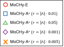
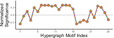
(a) email-EU

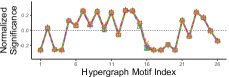
(b) contact-primary

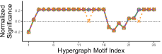
(c) coauth-history

Figure 9: Using MoCHy-A⁺, characteristic profiles (CPs) can be estimated accurately from a small number of samples.

5 Related Work

We review prior work on network motifs, algorithms for counting them, and hypergraphs. While the definition of a network motif varies among studies, here we define it as a connected graph composed by a predefined number of nodes.

Network Motifs. Network motifs were proposed as a tool for understanding the underlying design principles and capturing the local structural patterns of graphs [26, 55, 46]. The occurrences of motifs in real-world graphs are significantly different from those in random graphs [46], and they vary also depending on the domains of graphs [45]. The concept of network motifs has been extended to various types of graphs, including dynamic [49], bipartite [16], and heterogeneous [51] graphs. The occurrences of network motifs have been used in a wide range of graph applications: community detection [13, 68, 43, 62], ranking [73], graph embedding [52, 71], and graph neural networks [39], to name a few.

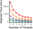
(a) Elapsed Time

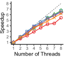
(b) Speedup

Figure 10: Both MoCHy-E and MoCHy-A⁺ achieve significant speedups with multiple threads.

Algorithms for Network Motif Counting. We focus on algorithms for counting the occurrences of every network motif whose size is fixed or within a certain range [4, 5, 9, 18, 21, 25, 50], while many are for a specific motif (e.g., the clique of size $3$) [3, 22, 27, 28, 31, 36, 38, 48, 54, 56, 57, 61, 63, 65]. Given a graph, they aim to count rapidly and accurately the instances of motifs with $4$ or more nodes, despite the combinatorial explosion of the instances, using the following techniques:

1. Combinatorics: For exact counting, [4, 50, 49] employ combinatorial relations between counts. That is, they deduce the counts of the instances of motifs from those of other smaller or equal-size motifs.

2. MCMC: Most approximate algorithms sample motif instances from which they estimate the counts. Employed MCMC sampling, [15, 21, 25, 53, 64] perform a random walk over instances (i.e, connected subgraphs) until it reaches the stationarity to sample an instance from a fixed probability distribution (e.g., uniform).

3. Color Coding: Instead of MCMC, [17, 18] employ color coding [7]. Specifically, they color each node uniformly at random among $k$ colors, count the number of $k$-trees with $k$ colors rooted at each node, and use them to sample instances from a fixed probability distribution.

In our problem, which focuses on h-motifs with only $3$ hyperedges, sampling instances with fixed probabilities is straightforward without (2) or (3), and the combinatorial relations on graphs in (1) are not applicable. In algorithmic aspects, we address the computational challenges discussed at the beginning of Section 3 by answering (a) what to precompute (Section 3.1), (b) how to leverage it (Sections 3.2 and 3.3), and (c) how to prioritize it (Sections 3.4 and 4.5), with formal analyses (Lemma 2; Theorems 1, 3, and 5).

Hypergraph. Hypergraphs naturally represent group interactions occurring in a wide range of fields, including computer vision [29, 70], bioinformatics [30], circuit design [34, 47], social network analysis [41, 67], and recommender systems [19, 42]. There also has been considerable attention on machine learning on hypergraphs, including clustering [2, 8, 35, 74], classification [32, 60, 70] and hyperedge prediction [12, 69, 72]. Recent studies on real-world hypergraphs revealed interesting patterns commonly observed across domains, including global structural properties (e.g., giant connected components and small diameter) [23] and temporal patterns regarding arrivals of the same or similar hyperedges [14]. Notably, Benson et al. [12] studied how several local features, including edge density, average degree, and probabilities of simplicial closure events for $4$ or less nodes, differ across domains. Our analysis using h-motifs is complementary to these approaches in that it (1) captures local patterns systematically without hand-crafted features, (2) captures static patterns without relying on temporal information, and (3) naturally uses hyperedges with any number of nodes without decomposing them into small ones.

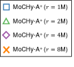
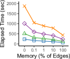
(a) Elapsed Time

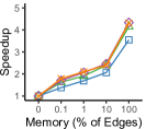
(b) Speedup

Figure 11: Memoizing a small fraction of projected graphs leads to significant speedups of MoCHy-A⁺.

6 Conclusions

In this work, we introduce hypergraph motifs (h-motifs), and using them, we investigate the local structures of $11$ real-world hypergraphs from $5$ different domains. We summarize our contributions as follows:

• Novel Concepts: We define 26 h-motifs, which describe connectivity patterns of three connected hyperedges in a unique and exhaustive way, independently of the sizes of hyperedges (Figure 3).

• Fast and Provable Algorithms: We propose $3$ parallel algorithms for (approximately) counting every h-motif’s instances, and we theoretically and empirically analyze their speed and accuracy. Both approximate algorithms yield unbiased estimates (Theorems 2 and 4), and especially the advanced one is up to $32\times$ faster than the exact algorithm, with little sacrifice on accuracy (Figure 8).

• Discoveries in $11$ Real-world Hypergraphs: We confirm the efficacy of h-motifs by showing that local structural patterns captured by them are similar within domains but different across domains (Figures 5 and 6).

Reproducibility: The code and datasets used in this work are available at https://github.com/geonlee0325/MoCHy.

Future directions include extending h-motifs to rich hypergraphs, such as temporal or heterogeneous hypergraphs, and incorporating h-motifs into various tasks, such as hypergraph embedding, ranking, and clustering.

Acknowledgements. This work was supported by National Research Foundation of Korea (NRF) grant funded by the Korea government (MSIT) (No. NRF-2020R1C1C1008296). This work was also supported by Institute of Information & Communications Technology Planning & Evaluation (IITP) grant funded by the Korea government (MSIT) (No. 2019-0-00075, Artificial Intelligence Graduate School Program (KAIST)) and supported by the National Supercomputing Center with supercomputing resources including technical support (KSC-2020-INO-0004).

Appendix A Proof of Theorem 2

We let $X_{ij}[t]$ be a random variable indicating whether the $i$-th sampled hyperedge (in line 4 of Algorithm 4) is included in the $j$-th instance of h-motif $t$ or not. That is, $X_{ij}[t]=1$ if the hyperedge is included in the instance, and $X_{ij}[t]=0$ otherwise. We let $\bar{m}[t]$ be the number of times that h-motif $t$’s instances are counted while processing $s$ sampled hyperedges. That is,

$$\bar{m}[t]:=\sum_{i=1}^{s}\sum_{j=1}^{M[t]}X_{ij}[t].\vspace{-1.5mm}$$ (9)

Then, by lines 4-4 of Algorithm 4,

$$\bar{M}[t]=\bar{m}[t]\cdot\tfrac{|E|}{3s}.\vspace{-1mm}$$ (10)

Proof of the Bias of $\bar{M}[t]$ (Eq. (4)): Since each h-motif instance contains three hyperedges, the probability that each $i$-th sampled hyperedge is contained in each $j$-th instance of h-motif $t$ is

$$P[X_{ij}[t]=1]=\mathbb{E}[X_{ij}[t]]=\tfrac{3}{|E|}.\vspace{-0.5mm}$$ (11)

From linearity of expectation,

$$\mathbb{E}[\bar{m}[t]]=\sum_{i=1}^{s}\sum_{j=1}^{M[t]}\mathbb{E}[X_{ij}[t]]=\sum_{i=1}^{s}\sum_{j=1}^{M[t]}\frac{3}{|E|}=\frac{3s\cdot M[t]}{|E|}.\vspace{-0.5mm}$$

Then, by Eq. (10), $\mathbb{E}[\bar{M}[t]]=\tfrac{|E|}{3s}\cdot\mathbb{E}[\bar{m}[t]]=M[t]$. ∎

Proof of the Variance of $\bar{M}[t]$ (Eq. (5)): From Eq. (11) and $X_{ij}[t]=X_{ij}[t]^{2}$, the variance of $X_{ij}[t]$ is

$$\mathbb{V}\mathrm{ar}[X_{ij}[t]]=\mathbb{E}[X_{ij}[t]^{2}]-\mathbb{E}[X_{ij}[t]]^{2}=\frac{3}{|E|}-\frac{9}{|E|^{2}}.\vspace{-1mm}$$ (12)

Consider the covariance between $X_{ij}[t]$ and $X_{i^{\prime}j^{\prime}}[t]$. If $i=i^{\prime}$, then from Eq. (11),

$$\mathbb{C}\mathrm{ov}(X_{ij}[t],X_{i^{\prime}j^{\prime}}[t])=\mathbb{E}[X_{ij}[t]\cdot X_{ij^{\prime}}[t]]-\mathbb{E}[X_{ij}[t]]\mathbb{E}[X_{ij^{\prime}}[t]]$$

$$=P[X_{ij}[t]=1,X_{ij^{\prime}}[t]=1]-\mathbb{E}[X_{ij}[t]]\mathbb{E}[X_{ij^{\prime}}[t]]$$

$$=P[X_{ij}[t]=1]\cdot P[X_{ij^{\prime}}[t]=1|X_{ij}[t]=1]$$

$$\hskip 10.0pt-\mathbb{E}[X_{ij}[t]]\mathbb{E}[X_{ij^{\prime}}[t]]$$

$$=\frac{3}{|E|}\cdot\frac{l_{jj^{\prime}}}{3}-\frac{9}{|E|^{2}}=\frac{l_{jj^{\prime}}}{|E|}-\frac{9}{|E|^{2}},\vspace{-1mm}$$ (13)

where $l_{jj^{\prime}}$ is the number of hyperedges that the $j$-th and $j^{\prime}$-th instances share. However, since hyperedges are sampled independently (specifically, uniformly at random with replacement), if $i\neq i^{\prime}$, then $\mathbb{C}\mathrm{ov}(X_{ij}[t],X_{i^{\prime}j^{\prime}}[t])=0$. This observation, Eq. (9), Eq. (12), and Eq. (13) imply

$$\mathbb{V}\mathrm{ar}[\bar{m}[t]]=\mathbb{V}\mathrm{ar}[\sum_{i=1}^{s}\sum_{j=1}^{M[t]}X_{ij}[t]]$$

$$=\sum_{i=1}^{s}\sum_{j=1}^{M[t]}\mathbb{V}\mathrm{ar}[X_{ij}[t]]+\sum_{i=1}^{s}\sum_{j\neq j^{\prime}}\mathbb{C}\mathrm{ov}(X_{ij}[t],X_{ij^{\prime}}[t])$$

$$=s\cdot M[t]\cdot(\frac{3}{|E|}-\frac{9}{|E|^{2}})+s\sum_{l=0}^{2}p_{l}[t](\frac{l}{|E|}-\frac{9}{|E|^{2}}),\vspace{-1mm}$$

where $p_{l}[t]$ is the number of pairs of h-motif $t$’s instances sharing $l$ hyperedges. This and Eq. (10) imply Eq. (5). ∎

Appendix B Proof of Theorem 4

A random variable $Y_{ij}[t]$ denotes whether the $i$-th sampled hyperwedge (in line 5 of Algorithm 5) is included in the $j$-th instance of h-motif $t$. That is, $Y_{ij}[t]=1$ if the sampled hyperwedge is included in the instance, and $Y_{ij}[t]=0$ otherwise. We let $\hat{m}[t]$ be the number of times that h-motif $t$’ instances are counted while processing $r$ sampled hyperwedges. That is,

$$\hat{m}[t]:=\sum_{i=1}^{r}\sum_{j=1}^{M[t]}Y_{ij}[t]$$ (14)

We use $w[t]$ to denote the number of hyperwedges included in each instance of h-motif $t$. That is,

$$w[t]:=\begin{cases}2&\text{if h-motif $t$ is open,}\\ 3&\text{if h-motif $t$ is closed.}\end{cases}\vspace{-0.5mm}$$ (15)

Then, by lines 5-5 of Algorithm 5,

$$\hat{M}[t]=\hat{m}[t]\cdot\tfrac{1}{w[t]}\cdot\tfrac{|\wedge|}{r}.\vspace{-1mm}$$ (16)

Proof of the Bias of $\hat{M}[t]$ (Eq. (6)): Since each instance of h-motif $t$ contains $w[t]$ hyperwedges, the probability that each $i$-th sampled hyperwedge is contained in each $j$-th instance of h-motif $t$ is

$$P[Y_{ij}[t]=1]=\mathbb{E}[Y_{ij}[t]]=\tfrac{w[t]}{|\wedge|}.\vspace{-1mm}$$ (17)

From linearity of expectation,

$$\mathbb{E}[\hat{m}[t]]=\sum_{i=1}^{r}\sum_{j=1}^{M[t]}\mathbb{E}[Y_{ij}[t]]=\sum_{i=1}^{r}\sum_{j=1}^{M[t]}\frac{w[t]}{|\wedge|}=\frac{w[t]\cdot r\cdot M[t]}{|\wedge|}.\vspace{-0.5mm}$$

Then, by Eq. (16), $\mathbb{E}[\hat{M}[t]]=\mathbb{E}[\hat{m}[t]]\cdot\tfrac{1}{w[t]}\cdot\tfrac{|\wedge|}{r}=M[t]$. ∎

Proof of the Variance of $\hat{M}[t]$ (Eq. (7) and Eq. (8):
From Eq. (17) and $Y_{ij}[t]=Y_{ij}[t]^{2}$, the variance of each random variable $Y_{ij}[t]$ is

$$\mathbb{V}\mathrm{ar}[Y_{ij}[t]]=\mathbb{E}[Y_{ij}[t]^{2}]-\mathbb{E}[Y_{ij}[t]]^{2}=\frac{w[t]}{|\wedge|}-\frac{w[t]^{2}}{|\wedge|^{2}}.\vspace{-1mm}$$ (18)

Consider the covariance between $Y_{ij}[t]$ and $Y_{i^{\prime}j^{\prime}}[t]$. If $i=i^{\prime}$, then from Eq. (17),

$$\mathbb{C}\mathrm{ov}(Y_{ij}[t],Y_{i^{\prime}j^{\prime}}[t])=\mathbb{E}[Y_{ij}[t]\cdot Y_{ij^{\prime}}[t]]-\mathbb{E}[Y_{ij}[t]]\mathbb{E}[Y_{ij^{\prime}}[t]]$$

$$=P[Y_{ij}[t]=1,Y_{ij^{\prime}}[t]=1]-\mathbb{E}[Y_{ij}[t]]\mathbb{E}[Y_{ij^{\prime}}[t]]$$

$$=P[Y_{ij}[t]=1]\cdot P[Y_{ij^{\prime}}[t]=1|Y_{ij}[t]=1]-\mathbb{E}[Y_{ij}[t]]\mathbb{E}[Y_{ij^{\prime}}[t]]$$

$$=\frac{w[t]}{|\wedge|}\cdot\frac{n_{jj^{\prime}}}{w[t]}-\frac{w[t]^{2}}{|\wedge|^{2}}=\frac{n_{jj^{\prime}}}{|\wedge|}-\frac{w[t]^{2}}{|\wedge|^{2}},\vspace{-0.5mm}$$ (19)

where $n_{jj^{\prime}}$ is the number of hyperwedges that the $j$-th and $j^{\prime}$-th instances share. However, since hyperwedges are sampled independently (specifically, uniformly at random with replacement), if $i\neq i^{\prime}$, then $\mathbb{C}\mathrm{ov}(Y_{ij}[t],Y_{i^{\prime}j^{\prime}}[t])=0$. This observation, Eq. (14), Eq. (18), and Eq. (19) imply

$$\mathbb{V}\mathrm{ar}[\hat{m}[t]]=\mathbb{V}\mathrm{ar}[\sum_{i=1}^{r}\sum_{j=1}^{M[t]}Y_{ij}[t]]$$

$$=\sum_{i=1}^{r}\sum_{j=1}^{M[t]}\mathbb{V}\mathrm{ar}[Y_{ij}[t]]+\sum_{i=1}^{r}\sum_{j\neq j^{\prime}}\mathbb{C}\mathrm{ov}(Y_{ij}[t],Y_{ij^{\prime}}[t])$$

$$=r\cdot M[t]\cdot(\frac{w[t]}{|\wedge|}-\frac{w[t]^{2}}{|\wedge|^{2}})+r\sum_{n=0}^{1}q_{n}[t]\cdot(\frac{n}{|\wedge|}-\frac{w[t]^{2}}{|\wedge|^{2}}),\vspace{-1mm}$$

where $q_{n}[t]$ is the number of pairs of h-motif $t$’s instances that share $n$ hyperwedges. This and Eq. (16) imply Eq. (7) and Eq. (8). ∎

References

- [1] Supplementary document. Available online: https://github.com/geonlee0325/MoCHy, 2020.
- [2] S. Agarwal, J. Lim, L. Zelnik-Manor, P. Perona, D. Kriegman, and S. Belongie. Beyond pairwise clustering. In CVPR, 2005.
- [3] N. K. Ahmed, N. Duffield, T. L. Willke, and R. A. Rossi. On sampling from massive graph streams. PVLDB, 10(11):1430–1441, 2017.
- [4] N. K. Ahmed, J. Neville, R. A. Rossi, and N. Duffield. Efficient graphlet counting for large networks. In ICDM, 2015.
- [5] N. K. Ahmed, J. Neville, R. A. Rossi, N. G. Duffield, and T. L. Willke. Graphlet decomposition: Framework, algorithms, and applications. Knowledge and Information Systems, 50(3):689–722, 2017.
- [6] S. G. Aksoy, T. G. Kolda, and A. Pinar. Measuring and modeling bipartite graphs with community structure. Journal of Complex Networks, 5(4):581–603, 2017.
- [7] N. Alon, R. Yuster, and U. Zwick. Color-coding. JACM, 42(4):844–856, 1995.
- [8] I. Amburg, N. Veldt, and A. R. Benson. Hypergraph clustering with categorical edge labels. In WWW, 2020.
- [9] C. Aslay, M. A. U. Nasir, G. De Francisci Morales, and A. Gionis. Mining frequent patterns in evolving graphs. In CIKM, 2018.
- [10] A.-L. Barabási and R. Albert. Emergence of scaling in random networks. science, 286(5439):509–512, 1999.
- [11] L. Becchetti, P. Boldi, C. Castillo, and A. Gionis. Efficient algorithms for large-scale local triangle counting. TKDD, 4(3):1–28, 2010.
- [12] A. R. Benson, R. Abebe, M. T. Schaub, A. Jadbabaie, and J. Kleinberg. Simplicial closure and higher-order link prediction. PNAS, 115(48):E11221–E11230, 2018.
- [13] A. R. Benson, D. F. Gleich, and J. Leskovec. Higher-order organization of complex networks. Science, 353(6295):163–166, 2016.
- [14] A. R. Benson, R. Kumar, and A. Tomkins. Sequences of sets. In KDD, 2018.
- [15] M. A. Bhuiyan, M. Rahman, M. Rahman, and M. Al Hasan. Guise: Uniform sampling of graphlets for large graph analysis. In ICDM, 2012.
- [16] S. P. Borgatti and M. G. Everett. Network analysis of 2-mode data. Social networks, 19(3):243–270, 1997.
- [17] M. Bressan, F. Chierichetti, R. Kumar, S. Leucci, and A. Panconesi. Counting graphlets: Space vs time. In WSDM, 2017.
- [18] M. Bressan, S. Leucci, and A. Panconesi. Motivo: fast motif counting via succinct color coding and adaptive sampling. PVLDB, 12(11):1651–1663, 2019.
- [19] J. Bu, S. Tan, C. Chen, C. Wang, H. Wu, L. Zhang, and X. He. Music recommendation by unified hypergraph: combining social media information and music content. In MM, 2010.
- [20] L. Chen, X. Qu, M. Cao, Y. Zhou, W. Li, B. Liang, W. Li, W. He, C. Feng, X. Jia, et al. Identification of breast cancer patients based on human signaling network motifs. Scientific reports, 3:3368, 2013.
- [21] X. Chen, Y. Li, P. Wang, and J. C. Lui. A general framework for estimating graphlet statistics via random walk. PVLDB, 10(3):253–264, 2016.
- [22] L. De Stefani, A. Epasto, M. Riondato, and E. Upfal. Trièst: Counting local and global triangles in fully-dynamic streams with fixed memory size. In KDD, 2016.
- [23] M. T. Do, S.-e. Yoon, B. Hooi, and K. Shin. Structural patterns and generative models of real-world hypergraphs. In KDD, 2020.
- [24] M. Faloutsos, P. Faloutsos, and C. Faloutsos. On power-law relationships of the internet topology. ACM SIGCOMM computer communication review, 29(4):251–262, 1999.
- [25] G. Han and H. Sethu. Waddling random walk: Fast and accurate mining of motif statistics in large graphs. In ICDM, 2016.
- [26] P. W. Holland and S. Leinhardt. A method for detecting structure in sociometric data. In Social Networks, pages 411–432. Elsevier, 1977.
- [27] X. Hu, Y. Tao, and C.-W. Chung. Massive graph triangulation. In SIGMOD, 2013.
- [28] X. Hu, Y. Tao, and C.-W. Chung. I/o-efficient algorithms on triangle listing and counting. TODS, 39(4):1–30, 2014.
- [29] Y. Huang, Q. Liu, S. Zhang, and D. N. Metaxas. Image retrieval via probabilistic hypergraph ranking. In CVPR, 2010.
- [30] T. Hwang, Z. Tian, R. Kuangy, and J.-P. Kocher. Learning on weighted hypergraphs to integrate protein interactions and gene expressions for cancer outcome prediction. In ICDM, 2008.
- [31] M. Jha, C. Seshadhri, and A. Pinar. A space efficient streaming algorithm for triangle counting using the birthday paradox. In KDD, 2013.
- [32] J. Jiang, Y. Wei, Y. Feng, J. Cao, and Y. Gao. Dynamic hypergraph neural networks. In IJCAI, 2019.
- [33] U. Kang, C. E. Tsourakakis, A. P. Appel, C. Faloutsos, and J. Leskovec. Radius plots for mining tera-byte scale graphs: Algorithms, patterns, and observations. In SDM, 2010.
- [34] G. Karypis, R. Aggarwal, V. Kumar, and S. Shekhar. Multilevel hypergraph partitioning: applications in vlsi domain. TVLSI, 7(1):69–79, 1999.
- [35] G. Karypis and V. Kumar. Multilevel k-way hypergraph partitioning. VLSI design, 11(3):285–300, 2000.
- [36] J. Kim, W.-S. Han, S. Lee, K. Park, and H. Yu. Opt: a new framework for overlapped and parallel triangulation in large-scale graphs. In SIGMOD, 2014.
- [37] B. Klimt and Y. Yang. The enron corpus: A new dataset for email classification research. In ECML PKDD, 2004.
- [38] S. Ko and W.-S. Han. Turbograph++ a scalable and fast graph analytics system. In SIGMOD, 2018.
- [39] J. B. Lee, R. A. Rossi, X. Kong, S. Kim, E. Koh, and A. Rao. Graph convolutional networks with motif-based attention. In CIKM, 2019.
- [40] J. Leskovec, J. Kleinberg, and C. Faloutsos. Graphs over time: densification laws, shrinking diameters and possible explanations. In KDD, 2005.
- [41] D. Li, Z. Xu, S. Li, and X. Sun. Link prediction in social networks based on hypergraph. In WWW, 2013.
- [42] L. Li and T. Li. News recommendation via hypergraph learning: encapsulation of user behavior and news content. In WSDM, 2013.
- [43] P.-Z. Li, L. Huang, C.-D. Wang, and J.-H. Lai. Edmot: An edge enhancement approach for motif-aware community detection. In KDD, 2019.
- [44] R. Mastrandrea, J. Fournet, and A. Barrat. Contact patterns in a high school: a comparison between data collected using wearable sensors, contact diaries and friendship surveys. PloS one, 10(9), 2015.
- [45] R. Milo, S. Itzkovitz, N. Kashtan, R. Levitt, S. Shen-Orr, I. Ayzenshtat, M. Sheffer, and U. Alon. Superfamilies of evolved and designed networks. Science, 303(5663):1538–1542, 2004.
- [46] R. Milo, S. Shen-Orr, S. Itzkovitz, N. Kashtan, D. Chklovskii, and U. Alon. Network motifs: simple building blocks of complex networks. Science, 298(5594):824–827, 2002.
- [47] M. Ouyang, M. Toulouse, K. Thulasiraman, F. Glover, and J. S. Deogun. Multilevel cooperative search for the circuit/hypergraph partitioning problem. TCAD, 21(6):685–693, 2002.
- [48] R. Pagh and C. E. Tsourakakis. Colorful triangle counting and a mapreduce implementation. Information Processing Letters, 112(7):277–281, 2012.
- [49] A. Paranjape, A. R. Benson, and J. Leskovec. Motifs in temporal networks. In WSDM, 2017.
- [50] A. Pinar, C. Seshadhri, and V. Vishal. Escape: Efficiently counting all 5-vertex subgraphs. In WWW, 2017.
- [51] R. A. Rossi, N. K. Ahmed, A. Carranza, D. Arbour, A. Rao, S. Kim, and E. Koh. Heterogeneous network motifs. arXiv preprint arXiv:1901.10026, 2019.
- [52] R. A. Rossi, N. K. Ahmed, and E. Koh. Higher-order network representation learning. In WWW Companion, 2018.
- [53] T. K. Saha and M. Al Hasan. Finding network motifs using mcmc sampling. In Complex Networks VI, pages 13–24. Springer, 2015.
- [54] S.-V. Sanei-Mehri, A. E. Sariyuce, and S. Tirthapura. Butterfly counting in bipartite networks. In KDD, 2018.
- [55] S. S. Shen-Orr, R. Milo, S. Mangan, and U. Alon. Network motifs in the transcriptional regulation network of escherichia coli. Nature genetics, 31(1):64–68, 2002.
- [56] K. Shin. Wrs: Waiting room sampling for accurate triangle counting in real graph streams. In ICDM, 2017.
- [57] K. Shin, S. Oh, J. Kim, B. Hooi, and C. Faloutsos. Fast, accurate and provable triangle counting in fully dynamic graph streams. TKDD, 14(2):1–39, 2020.
- [58] A. Sinha, Z. Shen, Y. Song, H. Ma, D. Eide, B.-J. Hsu, and K. Wang. An overview of microsoft academic service (mas) and applications. In WWW, 2015.
- [59] J. Stehlé, N. Voirin, A. Barrat, C. Cattuto, L. Isella, J.-F. Pinton, M. Quaggiotto, W. Van den Broeck, C. Régis, B. Lina, et al. High-resolution measurements of face-to-face contact patterns in a primary school. PloS one, 6(8), 2011.
- [60] L. Sun, S. Ji, and J. Ye. Hypergraph spectral learning for multi-label classification. In KDD, 2008.
- [61] C. E. Tsourakakis, U. Kang, G. L. Miller, and C. Faloutsos. Doulion: counting triangles in massive graphs with a coin. In KDD, 2009.
- [62] C. E. Tsourakakis, J. Pachocki, and M. Mitzenmacher. Scalable motif-aware graph clustering. In WWW, 2017.
- [63] P. Wang, P. Jia, Y. Qi, Y. Sun, J. Tao, and X. Guan. Rept: A streaming algorithm of approximating global and local triangle counts in parallel. In ICDE, 2019.
- [64] P. Wang, J. C. Lui, B. Ribeiro, D. Towsley, J. Zhao, and X. Guan. Efficiently estimating motif statistics of large networks. TKDD, 9(2):1–27, 2014.
- [65] P. Wang, Y. Qi, Y. Sun, X. Zhang, J. Tao, and X. Guan. Approximately counting triangles in large graph streams including edge duplicates with a fixed memory usage. PVLDB, 11(2):162–175, 2017.
- [66] D. J. Watts and S. H. Strogatz. Collective dynamics of ‘small-world’networks. nature, 393(6684):440, 1998.
- [67] D. Yang, B. Qu, J. Yang, and P. Cudre-Mauroux. Revisiting user mobility and social relationships in lbsns: A hypergraph embedding approach. In WWW, 2019.
- [68] H. Yin, A. R. Benson, J. Leskovec, and D. F. Gleich. Local higher-order graph clustering. In KDD, 2017.
- [69] S.-e. Yoon, H. Song, K. Shin, and Y. Yi. How much and when do we need higher-order information in hypergraphs? a case study on hyperedge prediction. In WWW, 2020.
- [70] J. Yu, D. Tao, and M. Wang. Adaptive hypergraph learning and its application in image classification. TIP, 21(7):3262–3272, 2012.
- [71] Y. Yu, Z. Lu, J. Liu, G. Zhao, and J.-r. Wen. Rum: Network representation learning using motifs. In ICDE, 2019.
- [72] M. Zhang, Z. Cui, S. Jiang, and Y. Chen. Beyond link prediction: Predicting hyperlinks in adjacency space. In AAAI, 2018.
- [73] H. Zhao, X. Xu, Y. Song, D. L. Lee, Z. Chen, and H. Gao. Ranking users in social networks with higher-order structures. In AAAI, 2018.
- [74] D. Zhou, J. Huang, and B. Schölkopf. Learning with hypergraphs: Clustering, classification, and embedding. In NIPS, 2007.