Generalized Gumbel-Softmax Gradient Estimator for Generic Discrete Random Variables

Abstract

Estimating the gradients of stochastic nodes in stochastic computational graphs is one of the crucial research questions in the deep generative modeling community, which enables the gradient descent optimization on neural network parameters. Stochastic gradient estimators of discrete random variables are widely explored, for example, Gumbel-Softmax reparameterization trick for Bernoulli and categorical distributions. Meanwhile, other discrete distribution cases such as the Poisson, geometric, binomial, multinomial, negative binomial, etc. have not been explored. This paper proposes a generalized version of the Gumbel-Softmax estimator, which is able to reparameterize generic discrete distributions, not restricted to the Bernoulli and the categorical. The proposed estimator utilizes the truncation of discrete random variables, the Gumbel-Softmax trick, and a special form of linear transformation. Our experiments consist of (1) synthetic examples and applications on VAE, which show the efficacy of our methods; and (2) topic models, which demonstrate the value of the proposed estimation in practice.

1 Introduction

Stochastic computational graphs, including variational autoencoders (VAEs) [1], are widely used for probabilistic modeling, representation learning, and generating data in the deep generative model (DGM) society. Optimizing the network parameters through back-propagating gradients requires an estimation of the gradient values. However, the stochasticity requires the computation of expectation, which differentiates this problem from the deterministic gradient of ordinary neural networks. Regarding such a perspective, there are two common ways of estimating the gradients from stochastic nodes: score function (SF) methods and reparameterization methods. The SF-based estimators tend to result in unbiased gradients with high variances, hence, the SF-based estimators aim to reduce the variances of gradients for stable and fast optimizations. Meanwhile, the reparameterization estimators result in biased gradients with low variances [2], but they require the differentiable non-centered parameterization [3] of random variables.

For continuous random variables such as the Gaussian, the reparameterization estimators are widely utilized due to the nature of the differentiability of the typical continuous distributions [1, 4, 5]. Nowadays, it is feasible to estimate gradients for continuous cases with automatic differentiation [6, 7] in TensorFlow [8] or PyTorch [9]. Meanwhile, for the discrete random variables which follow Bernoulli or categorical distributions, the SF-based methods are widely explored since the reparameterization method can not directly work due to the non-differentiability. Alternatively, the Gumbel-Softmax trick [10, 11] overcomes this difficulty through the reparameterization with continuous relaxation of one-hot selection values. Also, a line of works [12, 13] utilizes both the SF-based method and the reparameterization method.

While the Bernoulli and the categorical cases have been studied deeply, the gradient estimators for other discrete distributions have hardly been explored. There are several gradient estimators which are specialized in discrete distributions on combinatorial spaces, such as $k$-hot vector, permutation, and spanning trees on graphs [14, 15]. However, other renowned discrete distribution cases, such as Poisson, binomial, multinomial, geometric, negative binomial distributions, etc., have not been explored, which we mainly focus on in this paper. Prior works on probabilistic graphical models, such as Ranganath et al. [16, 17], adopted Poisson latent variables for latent counting. Another line of work [18] utilized the Gaussian approximation on the Poisson to count the number of words in deep generative modeling, which can be a poor approximation when the rate parameter is small. Regarding those perspectives, the stochastic gradient estimator for the discrete distribution needs to be studied further to extend the choice of prior assumptions.

This paper proposes a generalized version of the Gumbel-Softmax trick, which can reparameterize the broader ranges of discrete distributions, not limited to the Bernoulli and the categorical. The proposed Generalized Gumbel-Softmax (GenGS) is probabilistically grounded, and it utilizes (1) a truncation to finitize the infinite supports of the discrete distributions; and (2) a transformation that enables the generalization of the Gumbel-Softmax trick. Moreover, through the truncation, GenGS provides a posterior inference procedure that can be either explicit or implicit as a practical implementation. Our experiments show the efficacy with synthetic examples and VAEs, as well as the usability in topic model applications.

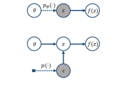
(a) Reparameterization trick.

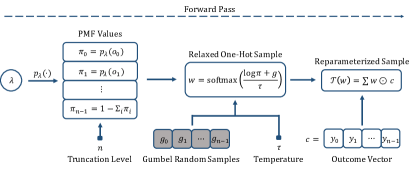
(b) Visualization of GenGS reparameterization trick.

Figure 1: Visualization of reparameterization trick. The shaded nodes indicate random nodes, and the dotted lines denote sampling processes. The auxiliary random variables enable the back-propagation flow of the gradients.

2 Preliminary

2.1 Back-propagation through Stochastic Nodes

In the stochastic computational graph, assume that there is an intermediate stochastic node or a latent variable $z\sim p(z|\theta)$, where the distribution depends on the parent node $\theta$ as a distribution parameter. The goal is optimizing the objective function $\mathcal{L(\theta,\eta)}=\mathds{E}_{z\sim p(z|\theta)}[f_{\eta}(z)]$, where $f_{\eta}$ is a differentiable function with respect to $\eta$, i.e., the neural networks. To optimize the objective function with respect to the parameter $\theta$ through the gradient methods, we need to compute $\nabla_{\theta}\mathcal{L(\theta,\eta)}=\nabla_{\theta}\mathds{E}_{z\sim p(z|\theta)}[f_{\eta}(z)]$, which is intractable with its original form.

SF-based estimator utilizes a score function $\nabla_{\theta}\log p(z|\theta)$ by utilizing log-derivative trick to compute the gradient $\nabla_{\theta}\mathcal{L(\theta,\eta)}$ [19]. Then, the gradient $\nabla_{\theta}\mathcal{L(\theta,\eta)}$ can be derived as the below:

$$\nabla_{\theta}\mathcal{L}(\theta,\eta)=\mathds{E}_{z\sim p(z|\theta)}[f_{\eta}(z)\nabla_{\theta}\log p(z|\theta)]~{}.$$ (1)

The SF methods compute exact gradients due to the unbiasedness with the Monte Carlo property. However, those methods suffer from the high variance of gradients, which results in the slow and unstable convergence of the objective function. To reduce the variance of gradients, the control variate methods [20, 21] or the RaoBlackwellization [22, 23] are widely used.

Reparameterization trick, illustrated in Figure 1(a), introduces an auxiliary variable $\epsilon\sim p(\epsilon)$, which takes over all randomness of the latent variable $z$, to compute $\nabla_{\theta}\mathcal{L(\theta,\eta)}$. Then, the sampled value $z$ can be re-written as $z=g(\theta,\epsilon)$, with a deterministic and differentiable function $g$ in terms of $\theta$. Here, the gradient $\nabla_{\theta}\mathcal{L(\theta,\eta)}$ is derived as the below:

$$\nabla_{\theta}\mathcal{L}(\theta,\eta)=\mathds{E}_{\epsilon\sim p(\epsilon)}[\nabla_{g}f_{\eta}(g(\theta,\epsilon))\nabla_{\theta}g(\theta,\epsilon)]~{}.$$ (2)

Equation (2) is computable, however, the differentiability requires the continuity of the random variable $z$, so the distribution of $z$ is limited to the continuous distributions.

2.2 Gumbel Tricks

To utilize the differentiable reparameterization trick on discrete random variables, continuous relaxation can be applied. A Gumbel-Softmax (GS) trick [10, 11] is an approximation of a Gumbel-Max (GM) trick, which are alternatives of a one-hot categorical sampling. The categorical random variable $Z\sim\text{Cat}(\pi)$, where $\pi$ in the $(n-1)$-simplex $\Delta^{n-1}$, can be reparameterized by the GM trick: (1) draw $u_{j}\sim\text{Uniform}(0,1)$ to generate a Gumbel sample $g_{j}=-\log(-\log{u_{j}})$ for $j=1,\cdots,n$; and (2) compute $k=\texttt{argmax}_{j=1}^{n}{[g_{j}+\log{\pi_{j}}]}$. This procedure generates a one-hot sample $z$ such that $z_{k}=1$ with $P(Z_{k}=1)=\pi_{k}$, and zeros in other entries. Instead of the argmax in the GM, the GS utilizes the softmax with a temperature $\tau>0$, i.e., $z\approx\texttt{softmax}\big{(}\frac{g+\log{\pi}}{\tau}\big{)}$. This substitution relaxes the discreteness of the categorical random variable to the one-hot-like form in the continuous domain. In other words, if we denote $\text{GM}(\pi)$ and $\text{GS}(\pi,\tau)$ as the distribution generated by the GM trick and the GS trick, respectively, then $\text{GS}(\pi,\tau)\rightarrow\text{GM}(\pi)$ as $\tau\rightarrow 0$.

3 Methodology

3.1 Problem Setting

We begin an explanation on GenGS with discrete distribution having finite support. Assume that a random variable $Z$ follows a discrete distribution $\text{Q}(\lambda)$ with explicit probability mass function (PMF) and a finite support $C=\{c_{1},\cdots,c_{n}\}$. Next, define an outcome vector $c=(c_{1},\cdots,c_{n})$ and the corresponding PMF value vector $\pi=(\pi_{1},\cdots,\pi_{n})$ in the same index order. Here, each sample $c_{k}$ can be either scalar or vector (or, even matrix) by the choice of distribution Q. Finally, for $w=(w_{1},\cdots,w_{n})\in\Delta^{n-1}$, introduce a transformation $\mathcal{T}$ as follows:

$$\textstyle\mathcal{T}(w)=\sum_{k=1}^{n}w_{k}c_{k}:=\sum w\odot c~{}.$$ (3)

3.2 Sampling through Generalized Gumbel Tricks

We claim that the sampling process of $Z$ can be derived by the one-hot categorical selection process, i.e., the GM process. Suppose that we draw a sample $Z=c_{k}\in C$, then the sampled value $c_{k}$ can be alternatively selected as follows. Since we fix the index order of the outcome vector $c$ and its corresponding PMF vector $\pi$, the one-hot indicating vector of the sample $c_{k}$ can be regarded as $w=\texttt{one\_hot}(c_{k}|c)$, which can be alternatively sampled from $\text{GM}(\pi)$. Then, the remaining step is a conversion of $w=\texttt{one\_hot}(c_{k}|c)$ to $c_{k}$, and this step can be done by the linear transformation $\mathcal{T}$ in Equation (3). Hence, we can reparameterize the original sample value $c_{k}$ as $\mathcal{T}(\text{GM}(\pi))$, as stated in Proposition 1.

Proposition 1.

For the transformation $\mathcal{T}$, if a discrete random variable $Z\sim\text{Q}(\lambda)$ has a finite support with known PMF values, $Z$ can be reparameterized by $\mathcal{T}(\text{GM}(\pi))$ where $\pi_{k}=P(Z=c_{k})$.

Proof.

With the transformation $\mathcal{T}$ and the constant outcome vector $c=(c_{1},\cdots,c_{n})$, the following holds:

$$c_{m}=\textstyle\sum_{k=1}^{n}c_{k}e_{k}=\mathcal{T}(e_{m})~{}.$$

Since the transformation $\mathcal{T}$ is a deterministic function, by introducing the auxiliary Gumbel random variable, we can remove the randomness of $Z$ from $\lambda$. Hence, the discrete random variable $Z$ with finite support can be reparameterized by the GM trick and the transformation $\mathcal{T}$. ∎

3.3 Relaxation of One-Hot Sample

Replacing the argmax in the GM trick to the softmax enables differentiation, which is a key point of the GS reparameterization. In Proposition 2, we claim that the same argument still holds under the transformation $\mathcal{T}$: if $W\sim\textsc{GS}(\pi,\tau)$ where $\pi$ is a PMF vector of discrete random variable $Z\sim\text{Q}(\lambda)$ with finite support, then $Z$ can be continuously relaxed and reparameterized as $\mathcal{T}(\textsc{GS}(\pi,\tau))$, which we define as $\textsc{GenGS}(\pi,\tau)$.

Proposition 2.

For the transformation $\mathcal{T}$ and a categorical parameter $\pi\in\Delta^{n-1}$, the convergence property of GS to GM still holds under the linear transformation $\mathcal{T}$, i.e., $\text{GS}(\pi,\tau)\rightarrow\text{GM}(\pi)$ as $\tau\rightarrow 0$ implies $\textsc{GenGS}(\pi,\tau)\rightarrow\mathcal{T}(\text{GM}(\pi))$ as $\tau\rightarrow 0$.

Proof.

Define $f_{M}$ and $f_{S}^{\tau}$ be GM reparameterization and GS reparameterization with a temperature $\tau>0$, respectively, where the both take the categorical parameter $\pi\in\Delta^{n-1}$ and a Gumbel sample as inputs. For the Gumbel sample $g$, if we assume $g_{m}+\log\pi_{m}>g_{j}+\log\pi_{j}$ for all $j\neq m$, then the following holds:

$$\mathcal{T}(f_{M}(\pi,g))=\textstyle\sum_{k=1}^{n}[e_{m}]_{k}\cdot c_{k}=\textstyle\sum_{k=1}^{n}e_{m}\odot c=c_{m}$$

where $e_{j}$ is a $n$-dimensional one-hot vector, which has $1$ in the $j^{\text{th}}$ entry and $0$ in all other entries. As $\tau\rightarrow 0$, the statement $\text{GS}(\pi,\tau)\rightarrow\text{GM}(\pi)$ implies $f_{S}^{\tau}(\pi,g)\rightarrow f_{M}(\pi,g)$, i.e.,

$$\big{[}f_{S}^{\tau}(\pi,g)\big{]}_{j} =\frac{\exp\big{(}\frac{g_{j}+\log\pi_{j}}{\tau}\big{)}}{\sum_{k=1}^{n}\exp\big{(}\frac{g_{k}+\log\pi_{k}}{\tau}\big{)}}\rightarrow\begin{cases}1&~{}\text{if}~{}j=m\\ 0&~{}\text{if}~{}j\neq m\end{cases}\quad\text{as}~{}\tau\rightarrow 0~{}.$$

Hence, $f_{S}^{\tau}(\pi,g)=\tilde{e}_{m}$ holds for some relaxed one-hot vector of $e_{m}$ by introducing the softmax relaxation. As a consequence,

$$\big{[}f_{S}^{\tau}(\pi,g)\big{]}_{j}\times c_{j} =\Big{[}\sum\frac{\exp\big{(}\frac{g_{i}+\log\pi_{i}}{\tau}\big{)}}{\sum_{k=1}^{n}\exp\big{(}\frac{g_{k}+\log\pi_{k}}{\tau}\big{)}}\Big{]}_{j}\times c_{j}$$

$$\rightarrow\begin{cases}c_{m}&~{}\text{if}~{}j=m\\ 0&~{}\text{if}~{}j\neq m\end{cases}\quad\text{as}~{}\tau\rightarrow 0~{}.$$

Hence, by taking the summation, the following holds:

$$\mathcal{T}(f_{S}^{\tau}(\pi,g))=\textstyle\sum_{k=1}^{n}[\tilde{e}_{m}]_{k}\cdot c_{k}\rightarrow c_{m}=\mathcal{T}(f_{M}(\pi,g))~{}.$$

∎

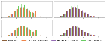
(a) Effects of truncation level and temperature

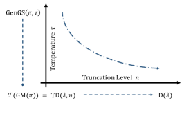
(b) Concept of GenGS approximation

Figure 2: (a) Approximation of GenGS in terms of choices of the truncation level $n$ and the temperature $\tau$ in $\text{Poisson}(7)$. As sub-figures go from left to right, the truncation level grows. Hence, the popped-out sticks, implying remaining probability of the right side, disappears if the truncation level is large enough. As sub-figures go from top to bottom, the temperature decreases, and the PMF of truncated distributions and the original distributions becomes similar. (b) On the $y$-axis, as temperature $\tau\downarrow 0$, $\textsc{GenGS}(\pi,\tau)\rightarrow\text{TD}(\lambda,n)$, where $\pi$ is a computed PMF value of $\text{TD}(\lambda,n)$, according to Proposition 2. $\text{TD}(\lambda,n)$ can be reparameterized by the GM trick with a linear transformation $\mathcal{T}$ as in Proposition 1. On the $x$-axis, $\text{TD}(\lambda,n)\rightarrow\text{D}(\lambda)$ as truncation level $n\uparrow\infty$, according to Proposition 4.

3.4 Finitizing Support by Truncation

In Section 3.1, we assumed that the support of the distribution to be finite. Without the finite assumption, the Gumbel tricks cannot be applied since it requires a limited number of categories. Hence, for the discrete distributions with infinite support, we truncate tails of the distributions to approximate the original distribution. In that manner, we can extend GenGS to the discrete distribution with infinite support. Definition 3 utilizes truncation range to truncate the non-negative discrete random variable.

Definition 3.

For a non-negative discrete random variable $X\sim\text{D}(\lambda)$, define $Z_{n}=X$ if $X\leq n-1$, and $Z_{n}=n-1$ if $X>n$. The random variable $Z_{n}$ is said to follow a truncated discrete distribution $\text{TD}(\lambda,R)$ with a parameter $\lambda$ and a truncation range $R=[0,n)$. Alternatively, we write as truncation level $R=n$ if the left truncation is at zero in the non-negative case.

Definition 3 not only finitizes the support but also provides the modification of the PMF: $\pi_{k}=P(Z_{n}=c_{k})=P(X=c_{k})$ for $k=1,\cdots,n-1$, and $\pi_{n}=P(Z_{n}=c_{n})=1-\sum_{k=1}^{n-1}\pi_{k}$. For the truncated random variable $Z_{n}\sim\text{TD}(\lambda,R)$ having an outcome vector $c=(c_{1},\cdots,c_{n})$, the ordering of $c_{k}$ is not significant, as long as the index of the outcome vector $c$ and the PMF vector $\pi$ are aligned. Proposition 4 provides a theoretical basis that $Z_{n}$ approximates $X$ as the truncation range widens enough. Hence, the truncation enables GenGS to be extendedly applied to the discrete distributions with infinite support such as the Poisson, geometric, negative binomial, etc. Similarly, Definition 3 and Proposition 4 can be generalized to general discrete distribution as Proposition 5 which we omit the proof.

Proposition 4.

$Z_{n}$ converges to $X$ almost surely as $n\rightarrow\infty$.

Proof.

Note that $\{\omega\in\Omega|Z_{n}(\omega)=X(\omega)\}=\{\omega\in\Omega|X(\omega)<n\}$. Then, we have the following:

$$P(\lim_{n\rightarrow\infty}Z_{n}=X) =P(\{\omega\in\Omega|\lim_{n\rightarrow\infty}Z_{n}(\omega)=X(\omega)\})$$

$$=P(\{\omega\in\Omega|\lim_{n\rightarrow\infty}Z_{n}(\omega)=\lim_{n\rightarrow\infty}X(\omega)<\lim_{n\rightarrow\infty}n\}\})$$

$$=P(\{\omega\in\Omega|X(\omega)<\infty\})=P(X<\infty)=1$$

since $X$ is a non-negative discrete random variable.∎

Proposition 5.

For a discrete random variable $X\sim\text{D}(\lambda)$, define (1) $Z_{m,n}=X$ if $m<X<n$; (2) $Z_{m,n}=n-1$ if $X\geq n$; and (3) $Z_{m,n}=m+1$ if $X\leq m$. Then, $Z_{m,n}$ converges to $X$ almost surely as $m\rightarrow-\infty$ and $n\rightarrow\infty$.

4 Hyper-Parameters & Variations of GenGS

Figure 1(b) illustrates the full steps of the GenGS trick, and Algorithm 1 shows the alternative sampling process of GenGS. Figure 2 describes how the GenGS trick approximates the original distribution by adjusting the temperature and the truncation range. The following are the hyper-parameter and the variations of the proposed GenGS.

Algorithm 1 Alternative sampling of GenGS with explicit PMF.

1:  Input: Distribution $\text{D}(\lambda)$ with PMF $p_{\lambda}(\cdot)$, finite possible outcome vector $c$ within truncation range $R$, temperature $\tau$.

2:  $\pi_{k}=p_{\lambda}(c_{k})$ for $k=1$ to $n-1$

3:  $\pi_{n}=1-\sum_{k=1}^{n-1}\pi_{k}$

4:  Draw Gumbel samples $g_{1},\cdots,g_{n}$.

5:  Compute ralaxed one-hot sample $w$ with $\textsc{GS}(\pi,\tau)$.

6:  Compute $z=\mathcal{T}(w)=\sum_{k=1}^{n}w\odot c$.

7:  return $z$

Temperature

Since GenGS utilizes the GS, GenGS inherits the temperature as a hyper-parameter. The decrement of temperature $\tau$ from results in the closer distribution to the original distribution. However, the initially small $\tau$ leads to high bias and variance of gradients, which becomes problematic at the learning stage on $\pi$. Hence, the annealing of $\tau$ from a large value to a small value is necessary to provide a learning chance of $\pi$.

Truncation Range

The truncated distribution becomes closer to the original distribution as we widen the truncation range $R$, and the choice of truncation range is crucial in terms of covering many probable samples or the modes of the distribution. Hence, we can set the truncation range to cover most of the support through a certain threshold. Also, for the popular discrete distributions such as Poisson, geometric, negative binomial, etc. which have a single mode in the PMF, we can use the mode as a criterion. Alternatively, we can set non-parameteric truncation range by thresholding, as in Algorithm 2.

Algorithm 2 GenGS NP: Computing PMF values without pre-defined truncation range.

1:  Input: Distribution $\text{D}(\lambda)$ with and PMF $p_{\lambda}(\cdot)$, temperature $\tau$, threshold $\eta\lesssim 1$.

2:  k, prob$\_$sum $=0,0$

3:  pi, c = list(), list()

4:  while prob$\_$sum $<\eta$ do

5:      pi.append($p_{\lambda}(\texttt{k})$), c.append(k)

6:      prob$\_$sum, k +=  $p_{\lambda}(\texttt{k}),1$

7:  pi.append(1-sum(pi)), c.append(k)

8:  return pi, c

Algorithm 3 GenGS Imp: GenGS with implicit PMF.

1:  Input: Distribution $\text{D}(\hat{\lambda})$ with inferred $\hat{\lambda}$, finite possible outcome vector $c$ within truncation range $R$, temperature $\tau$.

2:  $\hat{\pi}=\texttt{softmax}(\hat{\lambda})$

3:  Compute $z=\textsc{GenGS}(\hat{\pi},\tau)$.

4:  return $z$

5:  $\hat{\lambda}$ is further optimized by Proposition 6.

Implicit Inference

The stochastic gradient estimators or the alternative sampling with the reparameterization tricks are widely utilized for the sampling from some distribution after infering the distribution parameter. In such cases, there are distribution regularizer in the objective function, for example in VAEs, the KL divergence between the prior distribution and the approximate posterior distribution. To do so, we first infer the distribution parameter $\lambda$, and then the proposed GenGS can be utilized by computing the PMF values $\pi$ explicitly. However, we can instead directly infer the PMF values $\pi$ with softmax function, not through the distribution parameter $\lambda$. We name the two cases as explicit inference and implicit inference (GenGS Imp), respectively, and GenGS Imp becomes possible by truncating distribution due to the finiteness of the dimension in the softmax function with the neural networks. Although the implicit inference cannot directly infer the distribution parameter $\lambda$, we found that loosening the posterior shape leads to a significant performance gain in our VAE examples. Algorithm 3 presents GenGS Imp process.

Discretization

Straight-Through (ST) method [24, 10] can be applied to GenGS for drawing discrete samples. This variation samples discrete values in the feed-forward step, but utilizes the estimated gradient from the continuously relaxed and reparameterized GenGS in the back-propagation step. However, as in the original GS with the ST technique, GenGS with ST results in significant performance degradation in our synthetic examples.

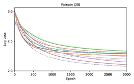
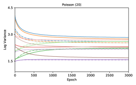
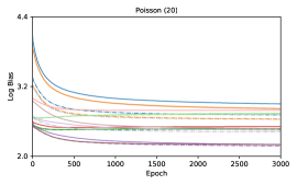
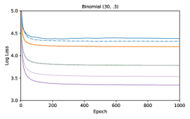
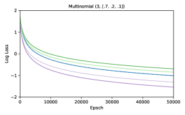
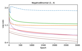
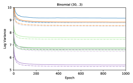
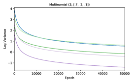
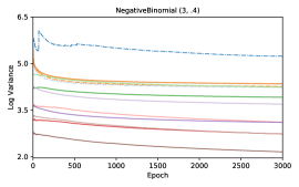
Figure 3: Synthetic example performance curves in log scale: (Top Row) losses, variances, and biases of gradients for Poisson; (Middle Row) losses for Binomial, Multinomial, and NegativeBinomial; (Bottom Row) variances of gradients for Binomial, Multinomial, and NegativeBinomial. We utilize the cumulative average for smoothing the curves following from Kool et al. [23].

5 Related Work

RF denotes the basic REINFORCE [19]. NVIL [20] utilizes a neural network to introduce the optimal control variate. MuProp [21] utilizes the first-order Taylor expansion on the objective function as a control variate. VIMCO [25] is designed as multi-sample gradient estimator. REBAR [12] and RELAX [13] utilize reparameterization trick for constructing the control variate. DetRB [22] uses the weighted value of the fixed gradients from $m$-selected categories and the estimated gradients from the remaining categories with respect to their odds to reduce the variance. The idea of StoRB [23] is essentially same as that of DetRB, but StoRB randomly chooses the categories at each step. Kool et al. [23] also suggested UnOrd, utilizing samples without replacements. Hence, DetRB, StoRB, and UnOrd can be considered as multi-sample gradient estimators. The ^∗ symbol denotes a built-in control variate introduced in the work of Kool et al. [23]. IRG [26] is an alternative of the GS and its variations can be applied to approximate the PMF including the Poisson, etc. However, IRG does not infer the distribution parameter as GenGS Imp, and the paper mainly focuses on replacing the GS rather than reparameterizing the general class of the discrete random variables.

Table 1: Training negative ELBO on MNIST and OMNIGLOT datasets. The lower is better for the negative ELBO, and the best and the second best results are marked in bold and underline, repecitvely. The symbol “—” indicates no convergence.

	Single-Sample Gradient Estimators								Multi-Sample (10) Gradient Estimators
MNIST	RF∗	NVIL	MuProp	REBAR	RELAX	GenGS	GenGS Imp	GenGS NP	VIMCO	StoRB∗	UnOrd	GenGS	GenGS Imp	GenGS NP
Pois(2)	$122.81_{\pm{2.41}}$	$129.34_{\pm{4.72}}$	$125.43_{\pm{2.27}}$	$123.44_{\pm{2.54}}$	$122.71_{\pm{1.92}}$	$\underline{103.18}_{\pm{0.92}}$	$\textbf{96.04}_{\pm{1.44}}$	$104.98_{\pm{1.19}}$	$122.13_{\pm{3.02}}$	$122.71_{\pm{3.83}}$	$130.95_{\pm{4.66}}$	$\underline{99.28}_{\pm{1.36}}$	$\textbf{94.78}_{\pm{1.17}}$	$102.59_{\pm{1.32}}$
Pois(3)	$123.12_{\pm{2.21}}$	$130.24_{\pm{3.32}}$	$125.92_{\pm{1.81}}$	$120.62_{\pm{2.31}}$	$119.84_{\pm{2.18}}$	$105.15_{\pm{1.71}}$	$\textbf{96.01}_{\pm{1.27}}$	$\underline{104.25}_{\pm{1.56}}$	$120.93_{\pm{2.48}}$	$121.92_{\pm{3.12}}$	$119.97_{\pm{5.38}}$	$\underline{100.17}_{\pm{1.73}}$	$\textbf{94.57}_{\pm{1.35}}$	$105.51_{\pm{1.80}}$
Geom(.25)	$127.90_{\pm{1.97}}$	$135.90_{\pm{2.38}}$	$137.90_{\pm{2.14}}$	$135.12_{\pm{2.74}}$	$136.80_{\pm{3.06}}$	$\underline{98.43}_{\pm{0.81}}$	$\textbf{92.52}_{\pm{1.62}}$	$101.77_{\pm{1.47}}$	$126.46_{\pm{2.22}}$	$130.96_{\pm{3.36}}$	—	$\underline{92.59}_{\pm{1.07}}$	$\textbf{92.06}_{\pm{0.78}}$	$100.34_{\pm{1.77}}$
Geom(.5)	$129.20_{\pm{2.03}}$	$138.47_{\pm{2.30}}$	$136.40_{\pm{1.78}}$	$138.37_{\pm{2.98}}$	$139.41_{\pm{3.59}}$	$100.92_{\pm{1.24}}$	$\textbf{93.81}_{\pm{1.60}}$	$\underline{97.29}_{\pm{1.89}}$	$128.71_{\pm{2.81}}$	$134.10_{\pm{4.65}}$	—	$98.27_{\pm{1.22}}$	$\textbf{91.46}_{\pm{0.95}}$	$\underline{96.44}_{\pm{1.38}}$
NB(3,.5)	$116.67_{\pm{5.97}}$	$119.28_{\pm{7.80}}$	$131.96_{\pm{6.49}}$	—	—	$\underline{98.58}_{\pm{1.27}}$	$\textbf{94.52}_{\pm{1.52}}$	$107.14_{\pm{2.14}}$	$112.11_{\pm{3.19}}$	$110.52_{\pm{2.21}}$	—	$\underline{96.83}_{\pm{1.63}}$	$\textbf{93.66}_{\pm{1.03}}$	$99.85_{\pm{1.91}}$
NB(5,.3)	$130.03_{\pm{3.99}}$	$133.44_{\pm{4.27}}$	$144.05_{\pm{8.15}}$	—	—	$\underline{100.88}_{\pm{2.35}}$	$\textbf{95.37}_{\pm{1.43}}$	$110.41_{\pm{2.81}}$	$121.29_{\pm{2.93}}$	$127.32_{\pm{4.79}}$	—	$\underline{97.29}_{\pm{1.87}}$	$\textbf{94.29}_{\pm{1.28}}$	$105.52_{\pm{2.53}}$
OMNIGLOT	RF∗	NVIL	MuProp	REBAR	RELAX	GenGS	GenGS Imp	GenGS NP	VIMCO	StoRB∗	UnOrd	GenGS	GenGS Imp	GenGS NP
Pois(2)	$139.47_{\pm{3.29}}$	$148.01_{\pm{4.19}}$	$142.95_{\pm{1.32}}$	$138.12_{\pm{3.26}}$	$137.56_{\pm{2.94}}$	$127.89_{\pm{1.44}}$	$\textbf{118.17}_{\pm{2.22}}$	$\underline{123.40}_{\pm{1.71}}$	$138.21_{\pm{3.29}}$	$137.87_{\pm{4.31}}$	$146.60_{\pm{4.97}}$	$\underline{120.42}_{\pm{2.21}}$	$\textbf{116.92}_{\pm{1.52}}$	$121.81_{\pm{2.47}}$
Pois(3)	$140.54_{\pm{2.36}}$	$148.13_{\pm{3.98}}$	$143.85_{\pm{1.54}}$	$137.92_{\pm{3.07}}$	$137.42_{\pm{2.96}}$	$131.53_{\pm{1.76}}$	$\textbf{119.15}_{\pm{1.92}}$	$\underline{126.03}_{\pm{2.16}}$	$138.84_{\pm{2.69}}$	$139.89_{\pm{3.98}}$	$147.18_{\pm{5.23}}$	$\underline{121.93}_{\pm{2.49}}$	$\textbf{117.71}_{\pm{1.28}}$	$124.71_{\pm{2.16}}$
Geom(.25)	$142.68_{\pm{2.96}}$	$153.69_{\pm{2.52}}$	$152.17_{\pm{1.77}}$	$146.78_{\pm{3.62}}$	$148.91_{\pm{4.03}}$	$\underline{115.23}_{\pm{2.00}}$	$\textbf{107.79}_{\pm{2.84}}$	$116.75_{\pm{1.90}}$	$142.42_{\pm{3.61}}$	$142.54_{\pm{3.21}}$	—	$\underline{113.49}_{\pm{1.95}}$	$\textbf{105.38}_{\pm{1.13}}$	$115.69_{\pm{2.03}}$
Geom(.5)	$142.70_{\pm{1.77}}$	$153.20_{\pm{1.49}}$	$149.76_{\pm{2.19}}$	$149.63_{\pm{3.49}}$	$151.97_{\pm{3.90}}$	$115.14_{\pm{2.43}}$	$\textbf{108.48}_{\pm{2.78}}$	$\underline{112.76}_{\pm{2.57}}$	$141.52_{\pm{3.38}}$	$140.68_{\pm{4.61}}$	—	$\underline{108.91}_{\pm{1.89}}$	$\textbf{105.97}_{\pm{1.30}}$	$112.41_{\pm{1.85}}$
NB(3,.5)	$141.44_{\pm{2.20}}$	$144.44_{\pm{2.78}}$	$147.78_{\pm{4.49}}$	—	—	$\underline{118.57}_{\pm{2.71}}$	$\textbf{117.02}_{\pm{2.18}}$	$123.96_{\pm{2.38}}$	$141.22_{\pm{3.42}}$	$128.66_{\pm{3.88}}$	—	$\underline{116.55}_{\pm{2.23}}$	$\textbf{114.20}_{\pm{1.61}}$	$120.92_{\pm{2.34}}$
NB(5,.3)	$145.16_{\pm{3.83}}$	$159.40_{\pm{5.13}}$	$152.81_{\pm{3.34}}$	—	—	$\underline{119.57}_{\pm{2.02}}$	$\textbf{117.54}_{\pm{2.76}}$	$127.46_{\pm{3.51}}$	$148.89_{\pm{4.51}}$	—	—	$\underline{118.37}_{\pm{2.51}}$	$\textbf{114.77}_{\pm{1.47}}$	$124.98_{\pm{2.95}}$

6 Experiment

6.1 Synthetic Example

Experimental Setting

This experiment expands the toy experiments from Tucker et al. [12], Grathwohl et al. [13] to diverse discrete distributions. We optimize the objective function $\mathds{E}_{z\sim p(z|\lambda)}\big{[}\sum_{i=1}^{k}(z_{i}-t_{i})^{2}\big{]}$ with respect to parameter $\lambda$ for fixed constants $t_{1},\cdots,t_{k}$. Here, we set distribution $p(z|\lambda)$ as $\text{Poisson}(\lambda)$, $\text{Binomial}(20,\lambda)$, $\text{Multinomial}(3,\lambda)$, and $\text{NegativeBinomial}(3,\lambda)$. For the Poisson and the negative binomial, which have infinite supports, we also applied Algorithm 2 to search the full range of support without pre-defined truncation range. Since the GenGSes are basically a single-sample gradient estimator, we utilize a single sample of $z$ for the fundamental comparison among the gradient estimators in the toy example.

Experimental Result

Figure 3 compares the log-loss and the log-variance of estimated gradients from various estimators. The log-loss needs to be minimized with the estimated gradient value in the learning process by back-propagation. Additionally, the log-variance requires being minimized to maintain the consistency of the gradients, so the gradient descent can be efficient. The GenGSes show the best log-loss and the best log-variance if the GenGSes keep the continuous relaxation of the modeled discrete random variable. For the Poisson, the exact gradient can be computed in closed-form, and the GenGSes show the lowest bias among all gradient estimators.

6.2 VAE: Synthetic Experiment on DGMs

Experimental Setting

To test the performance of the gradient estimators in DGMs, we adopt VAE which is one of the simplest DGMs. We follow the VAE experiment scheme of Figurnov et al. [6] which utilizes various prior distributions. In our discrete case, we utilize the Poisson (Pois), the geometric (Geom), and the negative binomial (NB) distributions, as the latent factor count. Note that the purpose of the VAE experiments is not to compare the performance across various prior distributions such as the categorical or the Gaussian, but to compare the performance across gradient estimators within the same prior distributions. The VAE is considered as a more challenging task than the synthetic example, since (1) this task requires computing the gradients of the encoder network parameters through the latent distribution parameter $\lambda$; and (2) each stochastic gradient of the latent dimension affects every encoder parameter since we are utilizing the fully-connected layers. Hence, a single poorly estimated gradient of the latent distribution parameter $\lambda$ could harm the learning of encoder parameters, so the VAE experiment can dynamically show the performance of the gradient estimators. Objective function of the VAE is the evidence lower bound (ELBO) $\mathcal{L}=\mathbb{E}_{q_{\phi(\mathbb{z}|\mathbb{x})}}[\log p_{\theta}(\mathbb{x}|\mathbb{z})]-\text{KL}(q_{\phi}(\mathbb{z}|\mathbb{x})||p_{\theta}(\mathbb{z}))$. In the GenGSes, by truncating the original distribution, the KL divergence between the approximate posterior and the prior distributions becomes the derivation with categorical distributions.

Proposition 6.

Assume two truncated distributions $X\sim\text{TD}(\lambda,n)$ and $Y\sim\text{TD}(\hat{\lambda},n)$ where $\pi_{k}=P(X=k)$, $\hat{\pi}_{k}=P(Y=k)$. Then, the KL divergence between $X$ and $Y$ can be represented in the KL divergence between the categorical distributions where $\text{KL}(Y||X)=\text{KL}(\text{Categorical}(\hat{\pi})||\text{Categorical}(\pi))$.

Proof.

$$\text{KL}(Y||X) =\textstyle\sum_{k}P(Y=k)\log{\bigg{(}\frac{P(Y=k)}{P(X=k)}\bigg{)}}=\textstyle\sum_{k}\hat{\pi}_{k}\log{\Big{(}\frac{\hat{\pi}_{k}}{\pi_{k}}\Big{)}}$$

$$=\text{KL}(\text{Categorical}(\hat{\pi})||\text{Categorical}(\pi))$$

∎

We separately compare the performance of the single-sample and multi-sample estimators with $10$ samples. For the GenGSes, we anneal the temperature from $1.$ to $.1$, and set truncation levels $12$ for $\text{Pois}(2)$; $15$ for $\text{Pois}(3)$; $25$ for $\text{Geom}(.25)$; $15$ for $\text{Geom}(.5)$; $30$ for $\text{NB}(3,.5)$; and $30$ for $\text{NB}(5,.3)$.

Experimental Result

To compare the estimators in the optimization perspective, Table 1 provides the training negative ELBO curves on MNIST and OMNIGLOT. DetRB, DetRB^∗, and StoRB are not listed since they hardly lead to the optimal point. The variants of GenGS showed the lowest negative ELBO in general for both the single and the multi cases. Also, loosening the PMF condition (i.e., the implicit inference) reached the better optimal points. The empirical reason why the implicit version is better than the explicit version is that the posterior PMF shape in the implicit case is thinner. Hence, the implicit distribution has a lower variance than the explicit one, and samples consistent values that lead to better trained neural network parameters, although it loses the original PMF shape.

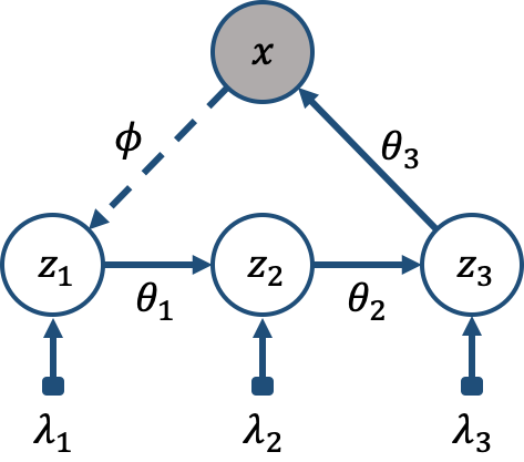
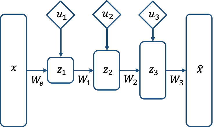
Figure 4: (Left) A graphical notation of NVPDEF with the generative ($\theta$) and the inference ($\phi$) processes. (Right) A neural network view of NVPDEF: diamond nodes indicate the auxiliary random variable for the reparameterization trick.

6.3 Application on Topic Model

Experimental Setting

This experiment shows practical usage of discrete distribution with GenGS in the deep generative topic modeling. The authors of Deep Exponential Families (DEFs) [16] utilized the exponential family on the stacked latent layers. We focus on the Poisson DEF, which assumes the Poisson latent layers to capture the count of latent super-topics and sub-topics. We convert the Poisson DEF into a neural variational form, which resembles NVDM [27], namely NVPDEF.

The generative and the inference process are

$$\text{Gen: }z_{k}\sim\text{Pois}(\lambda_{k-1})\text{ for }k=1,\cdots,K,\text{ and }x\sim\text{MLR}(\lambda_{K})$$

$$\text{Inf: }\hat{\lambda}_{0}=\text{MLP}(x),~{}\hat{\lambda}_{1}=W_{1}\hat{\lambda}_{0},~{}\cdots,~{}\hat{\lambda}_{K}=W_{K-1}\hat{\lambda}_{K-1}~{},$$

where MLR stands for multinomial logistic regression adopted from Miao et al. [27]. Each $z_{k}\sim\text{Poisson}(\lambda_{k-1})$ represents the count distribution of sub-topics from the super-topic, which is approximated by posterior $q(z_{k}|z_{k-1})=\text{Pois}(\hat{\lambda}_{k})$. Each component of $W_{k}$, $w_{k,i,j}$ is positive, and $w_{k,i,j}$ captures the positive weight of relationship between super-topic $i$ of the $k^{\text{th}}$ layer and sub-topic $j$ of the $(k+1)^{\text{th}}$ layer. Finally, NVPDEF optimizes

$$\mathcal{L}=\mathds{E}_{q(z_{1:K})}[\log p(x|z_{1:K})]\textstyle-\sum_{k=1}^{K}\text{KL}(q(z_{k}|z_{k-1})||p(z_{k}))$$ (4)

where $z_{0}=x$ for simplifying the equation. Figure 4 shows the graphical notation and the neural network structure.

For the single-stacked version of NVPDEF, we set $\lambda_{1}=.75$ with truncation level $15$ and fix the temperature as $\tau=.5$. For the multi-stacked version of NVPDEF, we set $\lambda_{1}=1.1,\lambda_{2}=1.$ with truncation level $15$. To have better chances of learning during the training period in the multi case, we utilize temperature annealing from $\tau=3.$ to $\tau=.5$, and multi-sample on the latent layers for the stable optimization of consecutive sampling. We compare the estimators by perplexity $\exp(-\frac{1}{D}\sum_{d}\frac{\log p(d)}{N_{d}})$ where $N_{d}$ is the number of words in document $d$, and $D$ is the total number of documents.

Table 2: NVPDEF test perplexity on 20Newsgroups and RCV1. $(m)$ in the model name indicates that $m$ samples are used for estimating the gradients. The lower is better for the perplexity, and the best results are marked in bold. The symbol “—” indicates no convergence.

Gradient Estimator	1-Stacked (Dim.)		Gradient Estimator	2-Stacked (Dim.)
	20News ($50$)	RCV1 ($200$)		20News ($50$)	RCV1 ($200$)
RF	$1227_{\pm{33.4}}$	$1182_{\pm{27.8}}$	RF$(10)$	—	—
RF∗	$944_{\pm{17.7}}$	$708_{\pm{15.6}}$	RF∗$(10)$	$1221_{\pm{19.6}}$	$2190_{\pm{30.9}}$
NVIL	$1077_{\pm{22.5}}$	$1191_{\pm{25.8}}$	NVIL$(10)$	—	—
MuProp	$1045_{\pm{20.1}}$	$935_{\pm{19.3}}$	MuProp$(10)$	—	—
VIMCO$(10)$	$958_{\pm{17.1}}$	$741_{\pm{16.2}}$	VIMCO$(20)$	—	—
REBAR	$934_{\pm{27.6}}$	$716_{\pm{25.9}}$	REBAR$(10)$	$1136_{\pm{26.3}}$	$2075_{\pm{43.6}}$
RELAX	$932_{\pm{31.1}}$	$717_{\pm{29.4}}$	RELAX$(10)$	$1116_{\pm{23.1}}$	—
StoRB∗$(10)$	$919_{\pm{16.2}}$	$701_{\pm{14.7}}$	StoRB∗$(20)$	$1094_{\pm{35.7}}$	—
UnOrd$(10)$	$1206_{\pm{24.3}}$	$1188_{\pm{22.1}}$	UnOrd$(20)$	—	—
GenGS	$\textbf{759}_{\pm{13.1}}$	$\textbf{562}_{\pm{11.5}}$	GenGS$(10)$	$\textbf{783}_{\pm{17.6}}$	$\textbf{576}_{\pm{18.8}}$

Experimental Result

We enumerate the results of NVPDEF with various gradient estimators in Table 2, and we confirmed that GenGS gives the lowest perplexity with 20Newsgroups and RCV1, which is aligned with the VAE results. Especially, the multi-stacked RCV1 case extremely shows the performance of the gradient estimators that many of the gradient estimators fail to reach the optimal point and GenGS gives the lowest perplexity.

7 Conclusion

This paper suggests variants of GenGS, a generalized version of the Gumbel-Softmax estimator, with the theoretical background. The synthetic analysis and the VAE experiment demonstrate the efficacy of GenGS, and the topic model application shows the usage of GenGS. The proposed GenGSes can be simply implemented, and the experimental result shows that the variants of GenGS lead to the better optimal point compared to existing stochastic gradient estimators. With the generalization, we expect that GenGS can diversify the options of distributions in the deep generative model community.

Declaration of Competing Interest

The authors declare that there are no conflicts of interest.

References

- Kingma and Welling [2014] D. P. Kingma, M. Welling, Auto-encoding variational bayes, International Conference on Learning Representations (2014).
- Xu et al. [2019] M. Xu, M. Quiroz, R. Kohn, S. A. Sisson, Variance reduction properties of the reparameterization trick, International Conference on Artificial Intelligence and Statistics (2019).
- Kingma and Welling [2014] D. P. Kingma, M. Welling, Efficient gradient-based inference through transformations between bayes nets and neural nets, International Conference on Machine Learning (2014).
- Nalisnick and Smyth [2017] E. Nalisnick, P. Smyth, Stick-breaking variational autoencoders, International Conference on Learning Representations (2017).
- Joo et al. [2020] W. Joo, W. Lee, S. Park, I. C. Moon, Dirichlet variational autoencoder, Pattern Recognition, 107, 107514 (2020).
- Figurnov et al. [2018] M. Figurnov, S. Mohamed, A. Mnih, Implicit reparameterization gradients, Advances in Neural Information Processing Systems (2018).
- Jankowiak and Obermeyer [2018] M. Jankowiak, F. Obermeyer, Pathwise derivatives beyond the reparameterization trick, International Conference on Machine Learning (2018).
- Abadi et al. [2016] M. Abadi, P. Barham, J. Chen, Z. Chen, A. Davis, J. Dean, M. Devin, S. Ghemawat, G. Irving, M. Isard, et al., Tensorflow: A system for large-scale machine learning, USENIX Symposium on Operating Systems Design and Implementation (2016).
- Paszke et al. [2019] A. Paszke, S. Gross, F. Massa, A. Lerer, J. Bradbury, G. Chanan, T. Killeen, Z. Lin, N. Gimelshein, L. Antiga, A. Desmaison, A. Kopf, E. Yang, Z. DeVito, M. Raison, A. Tejani, S. Chilamkurthy, B. Steiner, L. Fang, J. Bai, S. Chintala, Pytorch: An imperative style, high-performance deep learning library, Advances in Neural Information Processing Systems (2019).
- Jang et al. [2017] E. Jang, S. Gu, B. Poole, Categorical reparameterization with gumbel-softmax, International Conference on Learning Representations (2017).
- Maddison et al. [2017] C. J. Maddison, A. Mnih, Y. W. Teh, The concrete distribution: A continuous relaxation of discrete random variables, International Conference on Learning Representations (2017).
- Tucker et al. [2017] G. Tucker, A. Mnih, C. J. Maddison, J. Lawson, J. Sohl-Dickstein, Rebar: Low-variance, unbiased gradient estimates for discrete latent variable models, Advances in Neural Information Processing Systems (2017).
- Grathwohl et al. [2017] W. Grathwohl, D. Choi, Y. Wu, G. Roeder, D. Duvenaud, Backpropagation through the void: Optimizing control variates for black-box gradient estimation, International Conference on Learning Representations (2017).
- Gadetsky et al. [2020] A. Gadetsky, K. Struminsky, C. Robinson, N. Quadrianto, D. P. Vetrov, Low-variance black-box gradient estimates for the plackett-luce distribution, The Association for the Advancement of Artificial Intelligence (2020).
- Paulus et al. [2020] M. B. Paulus, D. Choi, D. Tarlow, A. Krause, C. J. Maddison, Gradient estimation with stochastic softmax tricks, Advances in Neural Information Processing Systems (2020).
- Ranganath et al. [2015] R. Ranganath, L. Tang, L. Charlin, D. Blei, Deep exponential families, Artificial Intelligence and Statistics (2015).
- Ranganath et al. [2016] R. Ranganath, A. Perotte, N. Elhadad, D. Blei, Deep survival analysis, Machine Learning for Healthcare Conference, PMLR (2016).
- Wu et al. [2020] J. Wu, Y. Rao, Z. Zhang, H. Xie, Q. Li, F. L. Wang, Z. Chen, Neural mixed counting models for dispersed topic discovery, Annual Meeting of the Association for Computational Linguistics (2020).
- Williams [1992] R. J. Williams, Simple statistical gradient-following algorithms for connectionist reinforcement learning, Machine Learning, 8(3-4), 229-256 (1992).
- Mnih and Gregor [2014] A. Mnih, K. Gregor, Neural variational inference and learning in belief networks, International Conference on Machine Learning (2014).
- Gu et al. [2016] S. Gu, S. Levine, I. Sutskever, A. Mnih, Muprop: Unbiased backpropagation for stochastic neural networks, International Conference on Learning Representations (2016).
- Liu et al. [2019] R. Liu, J. Regier, N. Tripuraneni, M. I. Jordan, J. McAuliffe, Rao-blackwellized stochastic gradients for discrete distributions, International Conference on Machine Learning (2019).
- Kool et al. [2020] W. Kool, H. van Hoof, M. Welling, Estimating gradients for discrete random variables by sampling without replacement, International Conference on Learning Representations (2020).
- Bengio et al. [2013] Y. Bengio, N. Leonard, A. Courville, Estimating or propagating gradients through stochastic neurons for conditional computation, arXiv preprint arXiv:1308.3432, (2013).
- Mnih and Rezende [2016] A. Mnih, D. J. Rezende, Variational inference for monte carlo objectives, International Conference on Machine Learning (2016).
- Potapczynski et al. [2020] A. Potapczynski, G. Loaiza-Ganem, J. P. Cunningham, Invertible gaussian reparameterization: Revisiting the gumbel-softmax, Advances in Neural Information Processing Systems (2020).
- Miao et al. [2016] Y. Miao, L. Yu, P. Blunsom, Neural variational inference for text processing, International Conference on Machine Learning (2016).