Robust Market Making via Adversarial Reinforcement Learning

Abstract

We show that adversarial reinforcement learning (ARL) can be used to produce market marking agents that are robust to adversarial and adaptively-chosen market conditions. To apply ARL, we turn the well-studied single-agent model of Avellaneda and Stoikov Avellaneda and Stoikov (2008) into a discrete-time zero-sum game between a market maker and adversary. The adversary acts as a proxy for other market participants that would like to profit at the market maker’s expense. We empirically compare two conventional single-agent RL agents with ARL, and show that our ARL approach leads to: 1) the emergence of risk-averse behaviour without constraints or domain-specific penalties; 2) significant improvements in performance across a set of standard metrics, evaluated with or without an adversary in the test environment, and; 3) improved robustness to model uncertainty. We empirically demonstrate that our ARL method consistently converges, and we prove for several special cases that the profiles that we converge to correspond to Nash equilibria in a simplified single-stage game.

1 Introduction

Market making refers to the act of providing liquidity to a market by continuously quoting prices to buy and sell a given financial instrument. The difference between these prices is called a spread, and the goal of a market maker (MM) is to repeatedly earn a spread by transacting in both directions. However, this is not done without risk. Market makers expose themselves to adverse selection, where toxic agents exploit their technological or informational edge, transacting with and thereby changing the MM’s inventory before an adverse price move causes them a loss. This is known as inventory risk, and has been the subject of a great deal of research in optimal control, artificial intelligence, and reinforcement learning (RL) literature.

A standard assumption in existing work has been that the MM has perfect knowledge of market conditions. Robustness of market making strategies to model ambiguity has only recently received attention - Cartea et al. (2017) extend optimal control approaches for the market making problem to address the risk of model misspecification. In this paper, we deal with this type of risk by taking an adversarial approach. We design market making agents that are robust to adversarial and adaptively chosen market conditions by applying adversarial RL. Our starting point is a well-known single-agent mathematical model of market making of Avellaneda and Stoikov (2008), which has been used extensively in the quantitative finance  Cartea et al. (2015, 2017); Guéant et al. (2011); Guéant (2017). We convert this into a discrete-time game, with a new “market player”, the adversary, that can be thought of as a proxy for other market participants that would like to profit at the expense of the market maker. The adversary controls dynamics of the market environment in a zero-sum game against the market maker.

We evaluate the sensitivity of RL-based strategies to three core parameters of the market model dynamics that affect prices and execution, where each of these parameters naturally varies over time in real markets. We thus go beyond the fixed parametrisation of existing models — henceforth called the Fixed setting — with two extended learning settings. The Random setting initialises each instance of the model (that is, episode in RL terminology) with values for the three parameters that are chosen independently and uniformly at random from three appropriate intervals. The Strategic setting features an adversary – an independent “market” learner whose objective is to choose the parameters from these same intervals so as to minimise the cumulative reward of the market maker in a zero-sum game. The Random and Strategic settings are, on the one hand, more realistic than the Fixed setting, but on the other hand, significantly more complex for the market making agent. We show that market making strategies trained in each of these settings yield significantly different behaviour, and we demonstrate striking benefits of our Strategic setting.

1.1 Contributions

The key contributions of this paper are as follows:

• We introduce a game-theoretic adaptation of a standard mathematical model of market making. Our adaption is useful to train robust MMs, and evaluate their performance in the presence of epistemic risk (Sections 2 and 3).

• We propose an algorithm for adversarial reinforcement learning in the spirit of RARL Pinto et al. (2017), and demonstrate its effectiveness in spite of the well known challenges associated with finding Nash equilibria of stochastic games Littman (1994) (Sections 4 and 5).

• We thoroughly investigate the impact of three environmental settings (one adversarial) on learning market making. We show that training against a Strategic adversary strictly dominates the other two settings (Fixed and Random) in terms of a set of standard desiderata, including the Sharpe ratio (Section 5).

• We prove that, in several key instances of the Strategic setting, the single-stage instantiation of our game has a Nash equilibrium resembling that found by our ARL algorithm for the multi-stage game. We then confirm broader existence of (approximate) equilibria in the multi-stage game by empirical best response computations (Sections 3 and 5).

1.2 Related Work

Optimal control and market making.

The theoretical study of market making originated from the pioneering work of Ho and Stoll (1981), Glosten and Milgrom (1985) and Grossman and Miller (1988), among others. Subsequent work focused on characterising optimal behaviour under different market dynamics and contexts. Most relevant is the work of Avellaneda and Stoikov (2008), who incorporated new insights into the dynamics of the limit order book to give a new market model, which is the one used in this paper. They derived closed-form expressions for the optimal strategy of an MM with an exponential utility function when the MM has perfect knowledge of the model and its parameters. This same problem was then studied for other utility functions Fodra and Labadie (2012); Guéant et al. (2011); Cartea et al. (2015); Cartea and Jaimungal (2015); Guéant (2017). As mentioned above, Cartea et al. (2017) study the impact of uncertainty in the model of Avellaneda and Stoikov Avellaneda and Stoikov (2008): they drop the assumption of perfect knowledge of market dynamics, and consider how an MM should optimally trade while being robust to possible misspecification. This type of epistemic risk is the primary focus of our paper.

Machine learning and market making.

Several papers have applied AI techniques to design automated market makers for financial markets. Chan and Shelton Chan and Shelton (2001) focussed on the impact of noise from uninformed traders on the quoting behaviour of a market maker trained with reinforcement learning. Abernethy and Kale Abernethy and Kale (2013) used an online learning approach. Spooner et al. Spooner et al. (2018) later explored the use of reinforcement learning to train inventory-sensitive market making agents in a fully data-driven limit order book model. Most recently, Guéant and Manziuk Guéant and Manziuk (2019) addressed scaling issues of finite difference approaches for high-dimensional, multi-asset market making using model-based RL. While the approach taken in this paper is also based on RL, unlike the majority of these works, our underlying market model is taken from the mathematical finance literature. There, models are typically analysed using methods from optimal control. We justify this choice in Section 2. To the best of our knowledge, we are the first to apply ARL to derive trading strategies that are robust to epistemic risk.

Risk-sensitive reinforcement learning.

Risk-sensitivity and safety in RL has been a highly active topic for some time. This is especially true in robotics where exploration is very costly. For example, Tamar et al. Tamar et al. (2012) studied policy search in the presence of variance-based risk criteria, and Bellemare et al. Bellemare et al. (2017) presented a technique for learning the full distribution of (discounted) returns; see also Garcıa and Fernández Garcıa and Fernández (2015). These techniques are powerful, but can be complex to implement and can suffer from numerical instability. This is especially true when using exponential utility functions which, without careful consideration, may diverge early in training due to large negative rewards Maddison et al. (2017). An alternative approach is to train agents in an adversarial setting Pinto et al. (2017); Pérolat et al. (2018) in the form of a zero-sum game. These methods tackle the problem of epistemic risk by explicitly accounting for the misspecification between train- and test-time simulations. This robustness to test conditions and adversarial disturbances is especially relevant in financial problems and motivated the approach taken in this paper.

2 Trading Model

We consider a standard model of market making as introduced by Avellaneda and Stoikov Avellaneda and Stoikov (2008) and studied by many others including Cartea et al. Cartea et al. (2017). The MM trades a single asset for which the price, $Z_{n}$, evolves stochastically. In discrete-time,

$$Z_{n+1}=Z_{n}+b_{n}\Delta t+\sigma_{n}W_{n},$$ (1)

where $b_{n}$ and $\sigma_{n}$ are the drift and volatility coefficients, respectively. The randomness comes from the sequence of independent, Normally-distributed random variables, $W_{n}$, each with mean zero and variance $\Delta t$. The process begins with initial value $Z_{0}=z$ and continues until step $N$ is reached.

The market maker interacts with the environment at each step by placing limit orders around $Z_{n}$ to buy or sell a single unit of the asset. The prices at which the MM is willing to buy (bid) and sell (ask) are denoted by $p_{n}^{+}$ and $p_{n}^{-}$, respectively, and may be expressed as offsets from $Z_{n}$:

$$\delta_{n}^{\pm}=\pm[Z_{n}-p_{n}^{\pm}]\geq 0;$$ (2)

these may be updated at each timestep at no cost to the agent. Equivalently, we may define:

$$\psi_{n} =\delta_{n}^{+}+\delta_{n}^{-}>0,$$ (3)

$$p_{n} =\frac{1}{2}(p_{n}^{+}+p_{n}^{-})=Z_{n}+\frac{1}{2}(\delta_{n}^{-}-\delta_{n}^{+}),$$

called the quoted spread and reservation price, respectively. These relate to the agent’s need for immediacy and bias in execution, amongst other things.

In a given time step, the probability that one or both of the agent’s limit orders are executed depends on the liquidity in the market and the values $\delta_{n}^{\pm}$. Transactions occur when market orders, which arrive at random times, have sufficient size to consume one of the agent’s limit orders. These interactions are modelled by independent Poisson processes, denoted by $N_{n}^{+}$ and $N_{n}^{-}$ for the bid and ask sides, respectively, with intensities $\lambda_{n}^{\pm}$; not to be confused with the terminal timestep $N$. The dynamics of the agent’s inventory process, or holdings, $H_{n}$, are then captured by the difference between these two terms,

$$H_{n}=(N_{n}^{+}-N_{n}^{-})\in[\underline{H},\overline{H}],$$ (4)

where $H_{0}$ is known and the values of $H_{n}$ are constrained so that trading stops on the opposing side of the book when either limit is reached. The order arrival intensities are given by:

$$\lambda_{n}^{\pm}=A_{n}^{\pm}e^{-k_{n}^{\pm}\delta_{n}^{\pm}},$$ (5)

where $A_{n}^{\pm},k_{n}^{\pm}>0$ describe the rate of arrival of market orders and distribution of volume in the book, respectively. This particular form derives from assumptions and observations on the structure and behaviour of limit order books which we omit here for simplicity; see Avellaneda and Stoikov (2008), Gould et al. (2013), and Abergel et al. (2016) for more details.

In this framework, the evolution of the market maker’s cash is given by the difference relation,

$$\begin{split}X_{n+1}&=X_{n}+p_{n}^{-}\Delta N_{n}^{-}-p_{n}^{+}\Delta N_{n}^{+},\\ &=X_{n}+\delta_{n}^{-}\Delta N_{n}^{-}+\delta_{n}^{+}\Delta N_{n}^{+}-Z_{n}\Delta H_{n},\end{split}$$ (6)

where $\Delta N_{n}^{\pm}\equiv N_{n+1}^{\pm}-N_{n}^{\pm}$. The cash flow is a combination of: the profit due to executing at the premium $\delta_{n}^{\pm}$, and the change in value of the agent’s holdings. The total value accumulated by the agent by timestep $n$ may thus be expressed as the sum of the cash held and value invested: $\Pi(X_{n},H_{n},Z_{n})$, where

$$\Pi(X,H,Z)=X+HZ,$$ (7)

and $\Pi_{n}\equiv\Pi(X_{n},H_{n},Z_{n})$. This is known as the mark-to-market (MtM) value of the agent’s portfolio.

Why not use a data driven approach?

Previous research into the use of RL for market making — and trading more generally — has focussed on data-driven limit order book models; see Nevmyvaka et al. (2006), Spooner et al. (2018), and Vyetrenko and Xu (2019). These methods, however, are not amenable to the type of analysis presented in Section 3. Using an analytical model allows us to examine the characteristics of adversarial training in isolation while minimising systematic error due to bias often present in historical data.

3 Game Formulation and Single-Stage Analysis

We use the market dynamics above to define a zero-sum stochastic game between a market maker and an adversary that acts as a proxy for all other market participants.

Definition 1.

[Market Making Game] The game between MM and an adversary has $N$ stages. At each stage, MM chooses $\delta^{\pm}$ and the adversary $\{b,A^{\pm},k^{\pm}\}$. The resulting stage payoff is given by expected change in MtM value of the MM’s portfolio, i.e., $\mathbb{E}[\Delta\Pi]$, see (7). The total payoff paid by the adversary to MM is the sum of the stage payoffs.

In the remainder of this section, we study theoretically the game when $N=1$, i.e., when there is a single stage. Later, in Section 5, we analyse empirically the game for $N=200$.

Single-stage analysis.

At each stage, the MM’s payoff may be unrolled to give:

$$f(\delta^{\pm};b,A^{\pm},k^{\pm})=\lambda^{+}\cdot(\delta^{+}+b)+\lambda^{-}\cdot(\delta^{-}-b)+bH.$$ (8)

For certain parameter ranges, this equation is concave in $\delta^{\pm}$.

Lemma 1 (Payoff Concavity in $\delta^{\pm}$).

The payoff (8) is a concave function of $\delta^{\pm}$ on the intervals $[0,\nicefrac{{2}}{{k}}-b]$, and $[0,\nicefrac{{2}}{{k}}+b]$, respectively.

Proof.

The first derivative of the payoff w.r.t. $\delta^{\pm}$ is given by:

$$\frac{\partial f}{\partial\delta^{\pm}}=\lambda^{\pm}\left[1-k(\delta^{\pm}\mp b)\right].$$ (9)

The Hessian matrix is thus given by,

$$\left\{\begin{matrix}k^{+}\lambda^{+}\left[k^{+}(\delta^{+}+b)-2\right]&0\\ 0&k^{-}\lambda^{-}\left[k^{-}(\delta^{-}-b)-2\right]\end{matrix}\right\},$$

which is negative semi-definite iff $\delta^{\pm}\leq\frac{2}{k^{\pm}}\mp b$. ∎

Note that (8) is linear in both $b$ and $A^{\pm}$. From this, we next show that there exists a Nash equilibrium (NE) when $\delta^{\pm}$ and $b$ are controlled, and $k^{\pm}$ and $A^{\pm}$ are fixed.

Theorem 1 (NE for fixed $A^{\pm},k^{\pm}$).

There is a pure strategy Nash equilibrium $(\delta^{\pm}_{\star},b_{\star})$ for $(\delta^{+},\delta^{-})\in[0,\nicefrac{{2}}{{k}}-b]\times[0,\nicefrac{{2}}{{k}}+b]$ and $b\in[\underline{b},\overline{b}]$ (with finite $\underline{b},\overline{b}$),

$$\delta_{\star}^{\pm}=\frac{1}{k}\pm b_{\star};\quad b_{\star}=\begin{cases}\underline{b}&\quad H>0,\\ \overline{b}&\quad H<0,\end{cases}$$ (10)

which is unique for $|H|>0$. When $H=0$, there is an equilibrium for every value $b_{\star}\in[\underline{b},\overline{b}]$.

Proof.

Equating (9) to zero and solving gives (10). To prove that these correspond to a pure strategy Nash Equilibrium of the game we show that the payoff is quasi-concave (resp. quasi-convex) in the MM’s (resp. adversary’s) strategy and then apply Sion’s minimax theorem Sion (1958). This follows from Lemma 1 for MM, and by the linearity of the adversary’s payoff w.r.t. $b$. For $|H|>0$, there is a unique solution. When $H=0$, there exists a continuum of solutions, all with equal payoff. ∎

The solution (10) has a similar form to that of the optimal strategy for linear utility with terminal inventory penalty Fodra and Labadie (2012), or equivalently that of a myopic agent with running penalty Cartea and Jaimungal (2015). Interestingly, the extension of Theorem 1 to an adversary with control over all three model parameters $\{b,A^{\pm},k^{\pm}\}$ yields a similar result. In this case we refer the reader the extended version of the paper spooner2020robust for a proof, and leave uniqueness to future work.

Theorem 2 (NE for general case).

There exists a pure strategy Nash equilibrium $(\delta^{\pm}_{\star},\{b_{\star},A^{\pm}_{\star},k^{\pm}_{\star}\})$ of the MM game for (10), $A^{\pm}_{\star}=\underline{A}$ and $k^{\pm}_{\star}=\overline{k}$.

4 Adversarial Training

The single-stage setting is informative but unrealistic. Next we investigate a range of multi-stage settings with various different restrictions on the adversary, and explore how adversarial training can improve the robustness of MM strategies. The following three types of adversary in turn increase the freedom of the adversary to control the market’s dynamics:

Fixed.

The simplest possible adversary always plays the same fixed strategy, for us: $b_{n}=0$, $A_{n}^{\pm}=140$ and $k_{n}^{\pm}=1.5$; these values match those originally used by Avellaneda and Stoikov Avellaneda and Stoikov (2008). This amounts to a single-agent learning setting with stationary transition dynamics.

Random.

The second type of adversary instantiates each episode with parameters chosen independently and uniformly at random from the following ranges: $b_{n}=b\in[-5,5]$, $A_{n}^{\pm}=A\in[105,175]$ and $k_{n}^{\pm}=k\in[1.125,1.875]$. These are chosen at the start of each episode and remain fixed until the terminal timestep $N$. This is analogous to single-agent RL with non-stationary transition dynamics.

Strategic.

The final type of adversary chooses the model parameters $b_{n},A_{n},k_{n}$ (bounded as in the previous setting) at each step of the game. This represents a fully-adversarial and adaptive learning environment, and unlike the models presented in related work Cartea et al. (2017), the source of risk here is exogenous and reactive to the quotes of the MM.

The principle of adversarial learning here — as with other successful applications Goodfellow et al. (2014) — is that if the MM plays a strategy that is not robust, then this can (and ideally will) be exploited by the adversary. If a Nash equilibrium (NE) strategy is played by MM then their strategy is robust and cannot be exploited. While there are no guarantees that a NE will be reached in our case, we show in Section 5 via empirical best response computations that our ARL method does consistently converge to reasonable approximate NE. Moreover, we show that we consistently outperform previous approaches in terms of absolute performance and robustness to model ambiguity.

Robustness through ARL was first introduced by Pinto et al. (2017) who demonstrated its effectiveness across a number of standard OpenAI gym domains. We adapt their RARL algorithm to support incremental actor-critic based methods and facilitate asynchronous training; though many of the features remain the same. The adversary is trained in parallel with the market maker, is afforded the same access to state — including MM’s inventory $H_{n}$ — and uses the same method for learning, which is described below.

4.1 Learning Configuration

Both agents use the NAC-S($\lambda$) algorithm, a natural actor-critic method Thomas (2014) for stochastic policies (i.e., mixed strategies) using semi-gradient SARSA($\lambda)$ Rummery and Niranjan (1994) for policy evaluation. The value functions are represented by compatible Peters and Schaal (2008) radial basis function networks of 100 Gaussian prototypes with accumulating eligibility traces Sutton and Barto (2018).

States.

The state of the environment $s_{n}=(t_{n},H_{n})$ contains only the current time $t_{n}=\frac{nT}{N}=n\Delta t$ and the agent’s inventory $H_{n}$, where the transition dynamics are governed by the definitions introduced in Section 2.

Policies.

The market maker learns a bivariate Normal policy for $\widetilde{p}_{n}\equiv p_{n}-S_{n}$ and $\psi_{n}$ with diagonal covariance matrix. The mean and variance vectors are modelled by linear function approximators using 3^rd-order polynomial bases Lagoudakis and Parr (2003). Both variances and the mean of the spread term, $\psi_{n}$, are kept positive via a softplus transformation. The adversary learns a Beta policy Chou et al. (2017), shifted and scaled to cover the market parameter intervals. The two shape parameters are learnt the same as for the variance of the Normal distribution above, with a translation of $+1$ to ensure unimodality and concavity.

Rewards.

The reward function is an adaptation of the optimisation objective of Cartea et al. (2017) and others, for the RL setting of incremental, discrete-time feedback:

$$R_{n}=\Delta\Pi_{n}-\zeta H_{n}^{2}-\begin{cases}0&\enskip\text{for }t<T,\\ \eta H_{n}^{2}&\enskip\text{otherwise},\end{cases}$$ (11)

where $\Pi_{n}$ refers to the MtM value of the agent’s holdings (Eq. 7). This formulation can be either risk-neutral (RN) or risk-adverse (RA). For example, if $\eta>0$ and $\zeta=0$, then the agent is punished if the terminal inventory $H_{N}$ is non-zero, and the solution becomes time-dependent. We refer to this case as RA and the case of $\eta=\zeta=0$ as RN.

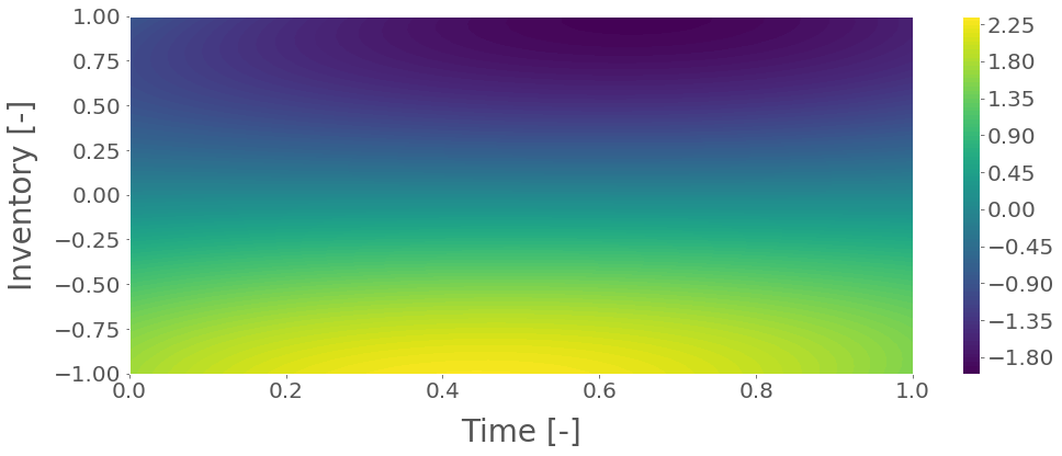
(a) Reservation price offset, $\widetilde{p}(t,H)$.

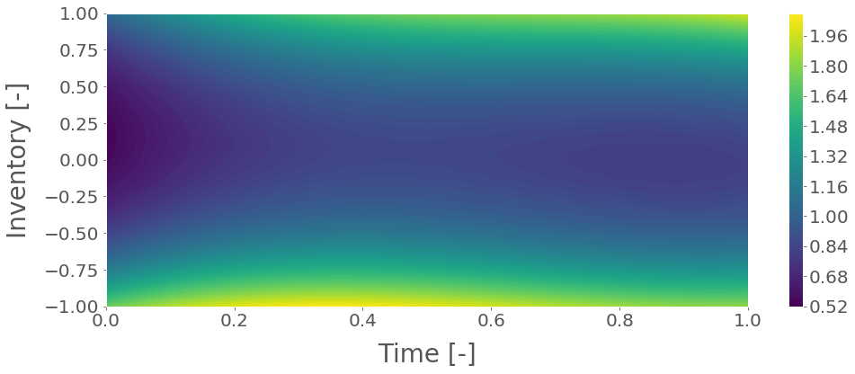
(b) Quoted spread, $\psi(t,H)$.

Figure 1: Most probable action for the risk-averse Gaussian policy learnt using NAC-S($\lambda$) with $\eta=0$ and $\zeta=0.01$.

$\eta$	$\zeta$	Term. wealth	Sharpe	Term. inventory	Avg. spread
0.0	0.0	$67.0\pm 12.0$	$5.57$	$0.56\pm 7.55$	$1.42\pm 0.02$
1.0	0.0	$61.3\pm 8.5$	$7.25$	$-0.04\pm 1.19$	$1.76\pm 0.02$
0.5	0.0	$63.0\pm 9.9$	$6.34$	$0.03\pm 1.24$	$1.67\pm 0.03$
0.1	0.0	$66.4\pm 9.4$	$7.06$	$-0.16\pm 1.86$	$1.42\pm 0.02$
0.01	0.0	$66.8\pm 11.1$	$6.00$	$0.87\pm 4.38$	$1.42\pm 0.02$
0.0	0.01	$63.4\pm 6.8$	$9.36$	$0.01\pm 1.45$	$1.60\pm 0.02$
0.0	0.001	$66.1\pm 7.4$	$8.94$	$0.15\pm 2.97$	$1.44\pm 0.02$

(a) Market makers trained against the Fixed adversary.

$\eta$	$\zeta$	Term. wealth	Sharpe	Term. inventory	Avg. spread
0.0	0.0	$66.7\pm 11.8$	$5.65$	$0.38\pm 7.14$	$1.36\pm 0.05$
1.0	0.0	$59.4\pm 7.6$	$7.79$	$0.02\pm 1.09$	$1.87\pm 0.02$
0.5	0.0	$62.9\pm 8.4$	$7.51$	$-0.04\pm 1.21$	$1.68\pm 0.02$
0.1	0.0	$65.8\pm 9.3$	$7.07$	$-0.18\pm 1.57$	$1.46\pm 0.03$
0.01	0.0	$66.6\pm 9.9$	$6.69$	$-0.65\pm 3.92$	$1.47\pm 0.02$
0.0	0.01	$64.0\pm 6.7$	$9.54$	$-0.06\pm 1.31$	$1.60\pm 0.02$
0.0	0.001	$65.9\pm 7.2$	$9.11$	$-0.07\pm 2.62$	$1.44\pm 0.02$

(b) Market makers trained against the Random adversary.

		Term. wealth	Sharpe	Term. inventory	Avg. spread
RN	$b$	$65.5\pm 6.9$	$9.51$	$0.04\pm 2.14$	$1.43\pm 0.01$
	$A^{\pm}$	$66.9\pm 13.1$	$5.11$	$2.45\pm 7.76$	$1.46\pm 0.02$
	$k^{\pm}$	$66.9\pm 12.7$	$5.27$	$0.52\pm 7.92$	$1.45\pm 0.02$
	$b,A^{\pm},k^{\pm}$	$65.1\pm 6.7$	$9.78$	$-0.05\pm 1.94$	$1.44\pm 0.02$
Full	$\eta=1.0$	$60.5\pm 6.8$	$8.88$	$-0.02\pm 0.97$	$1.75\pm 0.02$
	$\eta=0.5$	$63.3\pm 6.8$	$9.32$	$-0.07\pm 1.05$	$1.60\pm 0.01$
	$\eta=0.1$	$64.8\pm 6.7$	$9.72$	$-0.06\pm 1.37$	$1.49\pm 0.02$
	$\eta=0.01$	$65.0\pm 6.7$	$9.69$	$-0.08\pm 1.89$	$1.49\pm 0.01$
	$\zeta=0.01$	$62.9\pm 6.7$	$9.43$	$-0.03\pm 1.19$	$1.65\pm 0.02$
	$\zeta=0.001$	$64.3\pm 6.5$	$9.85$	$0.0\pm 1.71$	$1.44\pm 0.01$

(c) Market makers trained against a Strategic adversary.

Table 1: MM performance in terms of the standard desiderata. Each value was computed by evaluating the policy over $10^{5}$ episodes and computing the mean and sample standard deviation. Each test episode was generated with a Fixed adversary. Wealth and average spread are measured in units of “currency”; inventory in terms of units of the “asset”; and the Sharpe ratio is unitless.

5 Experiments

In each of the experiments to follow, the value function was pre-trained for 1000 episodes (with a learning rate of $10^{-3}$) to reduce variance in early policy updates. Both the value function and policy were then trained for $10^{6}$ episodes, with policy updates every 100 time steps, and a learning rate of $10^{-4}$ for both the critic and policy. The value function was configured to learn $\lambda=0.97$ returns. The starting time was chosen uniformly at random from the interval $t_{0}\in[0.0,0.95]$, with starting price $Z_{0}=100$ and inventory $H_{0}\in[\underline{H}=-50,\overline{H}=50]$. Innovations in $Z_{n}$ occurred with fixed volatility $\sigma=2$ between $[t_{0},1]$ with increment $\Delta t=0.005$.

5.1 Market Maker Desiderata

Market makers typically aim to maximise profits while controlling inventory and quoted spread. Higher terminal wealth with lower variance, less exposure to inventory risk and smaller spreads are all indicators of the risk aversion (or lack thereof) of a strategy. This is reflected in the majority of objective functions for market markers studied in the literature. We consider the following quantitative desiderata:

Profit and loss / Sharpe Ratio.

The distribution of a trading strategy’s profit and loss is the most fundamental object used to measure its performance. In our setup, we look at an agent’s distribution of episodic terminal wealth. In particular, we look at the moments $\mathbb{E}[\Pi_{N}]$ and $\mathbb{V}[\Pi_{N}]$ of this distribution, where the agent would like to maximise the former while minimising the latter. To this end, a common metric used in financial literature and in industry is the Shape ratio: $\frac{\mathbb{E}[\Pi_{N}]}{\mathbb{V}[\Pi_{N}]}$, in essence, the reward per unit of risk. While larger values are better, it is important to note that the Sharpe ratio is not a sufficient statistic.

Terminal inventory.

The distribution of terminal inventory, $H_{N}$, tells us about the robustness of the strategy to adverse price movements. In practice, it is desirable for a market maker to finish the trading day with small absolute values for $H_{N}$; though this is not always a strict requirement.

Quoted spread.

The “competitiveness” of a market maker is often discussed in terms of the average quoted spread: $\mathbb{E}_{n}[\psi_{n}]$. Tighter spreads imply more efficient markets and exchanges often compensate (with rebates) for smaller spreads.

5.2 Results

Fixed setting.

We first trained MMs against the Fixed adversary; i.e., a standard single-agent learning environment. Both RN and RA formulations of Eq. 11 were used with risk parameters $\eta\in\{1,0.5,0.1,0.01\}$ and $\zeta\in\{0.01,0.001\}$. Table 1(a) summarises the performance for the resulting agents. To provide some further intuition, we illustrate one of the learnt policies in Figure 1. In this case, the agent learnt to offset its price asymmetrically as a function of inventory, with increasing intensity as we approach the terminal time.

Random setting.

Next MMs were trained in an environment with a Random adversary; a simple extension to the training procedure that aims to develop robustness to epistemic risk. To compare with earlier results, the strategies were also tested against the Fixed adversary — a summary of which, for the same set of risk parameters, is given in Table 1(b). The impact on test performance in the face of model ambiguity was then evaluated by comparing market makers trained on the Fixed adversary with those trained against the Random adversary. Specifically, out-of-sample tests were carried out in an environment with a Random adversary. This means that the model dynamics at test-time were different from those at training time. While not explicitly adversarial, this misspecification of the model represents a non-trivial challenge for robustness. Overall, we found that market makers trained against the Fixed adversary exhibited no change in average wealth creation, but an increase of 98.1% in the variance across all risk parametrisations. On the other hand, market makers originally trained against the Random adversary yielded a lower average 86.0% increase in the variance. The Random adversary helps, but not by much compared with the Strategic adversary, as we will see next.

Strategic setting.

In this setting, we first consider an adversary that controls the drift $b$ only. With RN rewards, we found that the adversary learns a (time-independent) binary policy (Figure 2) that is identical to the strategy in the corresponding single-stage game; see Section 3. We also found that the strategy learnt by the MM in this setting generates profits and associated Sharpe ratios in excess of all other strategies seen thus far when tested against the Fixed adversary (see Table 1(c)). This is true also when comparing with tests run against the Random or Strategic adversaries, suggesting that the adversarially trained MM is indeed more robust to test-time model discrepancies.

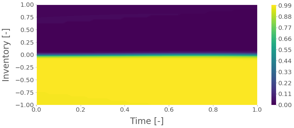
Figure 2: Policy learnt by the adversary for manipulating price against the market maker with $\eta=\zeta=0$.

This, however, does not extend to Strategic adversaries with control over either only $A^{\pm}$ or only $k^{\pm}$. In these cases, performance was found to be no better than the corresponding MMs trained in the Fixed setting with a conventional learning setup. The intuition for this again derives from the single-stage analysis. That is, the adversary almost surely chooses a strategy that minimises $A^{\pm}$ (equiv. maximises $k^{\pm}$) in order to decrease the probability of execution, thus decreasing MM’s profits derived from execution and MM’s ability to manage inventory effectively. The control afforded to the adversary must correlate in some way with sources of variance — such as inventory speculation — in order for robustness to correspond to practicable forms of risk-aversion.

Then the natural question is then whether an adversary with simultaneous control over $b,A^{\pm}$, and $k^{\pm}$ produces strategies outperforming those where the adversary controls $b$ alone. This is plausible since combining the three model parameters can lead to more interesting strategies, e.g., driving inventory up/down only to increase drift at the peak (i.e., pump and dump). We investigated by training an adversary with control over all three parameters. The resulting performance can be found in Table 1(c), which shows an improvement in the Sharpe ratio of 0.27 and lower variance on terminal wealth. Interestingly, these MMs also quote tighter spreads on average — the values even approaching that of the risk-neutral MM trained against a Fixed adversary. This indicates that the strategies are able to achieve epistemic risk aversion without charging more to counterparties.

Exploring the impact of varying risk parameters of the reward function, $\eta$ and $\zeta$ (see (11)), we found that in all cases MM strategies trained against a Strategic adversary with an RA reward outperformed their counterparts in Tables 1(a) and 1(b). It is unclear, however, if changes to the reward function away from the RN variant actually improved the strategy in general. Excluding when $\zeta=0.001$, all values appear to do worse than for an adversarially trained MM with RN reward. It may well be that the addition of inventory penalty terms actually boosts the power of the adversary and results in strategies that try to avoid trading at all, a frequent problem in this domain.

Verification of approximate equilibria.

Holding the strategy of one player fixed, we empirically computed the best response against it by training. We found consistently that neither the trader nor adversary deviated from their policy. This suggests that our ARL method were finding reasonable approximate Nash equilibria. While we do not provide a full theoretical analysis of the stochastic game, these findings are corroborated by those in Section 3, since, as seen in Figure 2, the learned policy in the multi-stage setting corresponds closely to the equilibrium strategy from the single-stage case that was presented in Section 3.

6 Conclusions

We introduced a new approach for learning trading strategies with ARL. The learned strategies are robust to the discrepancies between the market model in training and testing. We show that our approach leads to strategies that outperform previous methods in terms of PnL and Sharpe ratio, and have comparable spread efficiency. This is shown to be the case for out-of-sample tests in all three of the considered settings, Fixed, Random, and Strategic. In other words, our learned strategies are not only more robust to misspecification, but also dominate in overall performance.

In some special cases we show that the learned strategies correspond to Nash equilibria of the corresponding single-stage game. More widely, we empirically show that the learned strategies correspond to approximate equilibria in the multi-stage stochastic game.

In future we plan to:

1. Extend to oligopolies of market makers.

2. Apply to data-driven and multi-asset models.

3. Further explore existence of equilibria and design provably-convergent algorithms.

Finally, we remark that, while our paper focuses on market making, the approach can be applied to other trading scenarios such as optimal execution and statistical arbitrage, where we believe it is likely to offer similar benefits. Further, it is important to acknowledge that this methodology has significant implications for safety of RL in finance. Training strategies that are explicitly robust to model misspecification makes deployment in the real-world considerably more practicable.

Software.

All our code is freely accessible on GitHub: https://github.com/tspooner/rmm.arl.

References

- Abergel et al. [2016] F. Abergel, M. Anane, A. Chakraborti, A. Jedidi, and I. M. Toke. Limit Order Books. Cambridge University Press, 2016.
- Abernethy and Kale [2013] J. D. Abernethy and S. Kale. Adaptive Market Making via Online Learning. In Proc. of NIPS, pages 2058–2066, 2013.
- Avellaneda and Stoikov [2008] M. Avellaneda and S. Stoikov. High-frequency trading in a limit order book. Quantitative Finance, 8(3):217–224, 2008.
- Bellemare et al. [2017] M. G. Bellemare, W. Dabney, and R. Munos. A Distributional Perspective on Reinforcement Learning. In Proc. of ICML, pages 449–458, 2017.
- Cartea and Jaimungal [2015] Á. Cartea and S. Jaimungal. Order-Flow and Liquidity Provision. Available at SSRN 2553154, 2015.
- Cartea et al. [2015] Á. Cartea, S. Jaimungal, and J. Penalva. Algorithmic and High-Frequency Trading. Cambridge University Press, 2015.
- Cartea et al. [2017] Á. Cartea, R. Donnelly, and S. Jaimungal. Algorithmic Trading with Model Uncertainty. SIAM Journal on Financial Mathematics, 8(1):635–671, 2017.
- Chan and Shelton [2001] N. T. Chan and C. Shelton. An Electronic Market-Maker. 2001.
- Chou et al. [2017] P.-W. Chou, D. Maturana, and S. Scherer. Improving Stochastic Policy Gradients in Continuous Control with Deep Reinforcement Learning Using the Beta Distribution. In Proc. of ICML, pages 834–843, 2017.
- Fodra and Labadie [2012] P. Fodra and M. Labadie. High-frequency market-making with inventory constraints and directional bets. arXiv preprint arXiv:1206.4810, 2012.
- Garcıa and Fernández [2015] J. Garcıa and F. Fernández. A comprehensive survey on safe reinforcement learning. JMLR, 16(1):1437–1480, 2015.
- Glosten and Milgrom [1985] L. R. Glosten and P. R. Milgrom. Bid, Ask and Transaction Prices in a Specialist Market with Heterogeneously Informed Traders. Journal of Financial Economics, 14(1):71–100, 1985.
- Goodfellow et al. [2014] I. Goodfellow, J. Pouget-Abadie, M. Mirza, B. Xu, D. Warde-Farley, S. Ozair, A. Courville, and Y. Bengio. Generative Adversarial Nets. In Proc. of NIPS, pages 2672–2680, 2014.
- Gould et al. [2013] M. D. Gould, M. A. Porter, S. Williams, M. McDonald, D. J. Fenn, and S. D. Howison. Limit Order Books. Quantitative Finance, 13(11):1709–1742, 2013.
- Grossman and Miller [1988] S. J. Grossman and M. H. Miller. Liquidity and Market Structure. The Journal of Finance, 43(3):617–633, 1988.
- Guéant and Manziuk [2019] O. Guéant and I. Manziuk. Deep reinforcement learning for market making in corporate bonds: beating the curse of dimensionality. arXiv preprint arXiv:1910.13205, 2019.
- Guéant et al. [2011] O. Guéant, C.-A. Lehalle, and J. Fernandez-Tapia. Dealing with the Inventory Risk: A solution to the market making problem. Mathematics and Financial Economics, 7(4):477–507, 2011.
- Guéant [2017] O. Guéant. Optimal market making. Applied Mathematical Finance, 24(2):112–154, 2017.
- Ho and Stoll [1981] T. Ho and H. R. Stoll. Optimal Dealer Pricing Under Transactions and Return Uncertainty. Journal of Financial Economics, 9(1):47–73, 1981.
- Lagoudakis and Parr [2003] M. G. Lagoudakis and R. Parr. Least-Squares Policy Iteration. JMLR, 4:1107–1149, 2003.
- Littman [1994] M. L. Littman. Markov games as a framework for multi-agent reinforcement learning. In Proc. of ICML, pages 157–163. 1994.
- Maddison et al. [2017] C. J. Maddison, D. Lawson, G. Tucker, N. Heess, M. Norouzi, A. Mnih, A. Doucet, and Y. W. Teh. Particle Value Functions. In ICLR 2017 Workshop Proceedings, 2017.
- Nevmyvaka et al. [2006] Y. Nevmyvaka, Y. Feng, and M. Kearns. Reinforcement Learning for Optimized Trade Execution. In Proc. of ICML, pages 673–680. ACM, 2006.
- Othman [2012] A. Othman. Automated Market Making: Theory and Practice. PhD thesis, CMU, 2012.
- Pérolat et al. [2018] J. Pérolat, B. Piot, and O. Pietquin. Actor-Critic Fictitious Play in Simultaneous Move Multistage Games. In Proc. of AISTATS, 2018.
- Peters and Schaal [2008] J. Peters and S. Schaal. Natural Actor-Critic. Neurocomputing, 71(7-9):1180–1190, 2008.
- Pinto et al. [2017] L. Pinto, J. Davidson, R. Sukthankar, and A. Gupta. Robust Adversarial Reinforcement Learning. In Proc. of ICML, volume 70, pages 2817–2826, 2017.
- Rajeswaran et al. [2017] A. Rajeswaran, S. Ghotra, B. Ravindran, and S. Levine. EPOpt: Learning Robust Neural Network Policies using Model Ensembles. In Proc. of ICLR, 2017.
- Rummery and Niranjan [1994] G. A. Rummery and M. Niranjan. On-line Q-learning Using Connectionist Systems. Technical report, Department of Engineering, University of Cambridge, 1994.
- Sion [1958] M. Sion. On General Minimax Theorems. Pacific Journal of Mathematics, 8(1):171–176, 1958.
- Spooner et al. [2018] T. Spooner, J. Fearnley, R. Savani, and A. Koukorinis. Market Making via Reinforcement Learning. In Proc. of AAMAS, pages 434–442, 2018.
- Sutton and Barto [2018] R. S. Sutton and A. G. Barto. Reinforcement Learning: An Introduction. MIT Press, 2018.
- Tamar et al. [2012] A. Tamar, D. Di Castro, and S. Mannor. Policy Gradients with Variance Related Risk Criteria. In Proc. of ICML, pages 1651–1658, 2012.
- Thomas [2014] P. Thomas. Bias in Natural Actor-Critic Algorithms. In Proc. of ICML, volume 32, pages 441–448, 2014.
- Vyetrenko and Xu [2019] S. Vyetrenko and S. Xu. Risk-Sensitive Compact Decision Trees for Autonomous Execution in Presence of Simulated Market Response. arXiv preprint arXiv:1906.02312, 2019.