Accuracy of Difference Schemes in Electromagnetic Applications:
a Trefftz Analysis

Abstract

The paper examines local approximation errors of finite difference schemes in electromagnetic analysis. Despite a long history of the subject, several accuracy-related issues have been overlooked and/or remain controversial. For example, conflicting claims have been made in the literature about the order of Yee-like schemes in the vicinity of slanted or curved material interfaces. Two novel practical methods for comparison of local accuracy of difference schemes are proposed: one makes use of Trefftz test matrices, and the other one relies on a new measure of approximation accuracy in scheme-exact Trefftz subspaces. One particular conclusion is that a loss of accuracy for Yee-like schemes at slanted material boundaries is unavoidable.

I Introduction

Finite difference (FD) schemes have been known for over a century [1] and in computational electrodymanics have been extensively used since the publication of Yee’s paper [2] in 1966. Despite this long history, several principal issues related to the accuracy of various schemes are not yet resolved to the satisfaction of application engineers, developers and practitioners. These issues appear in the bulleted list of Section II; but to motivate the discussion, let us start with the following observations.

The Yee schemes on regular Cartesian grids are well known to be of second order in a homogeneous medium and also at material interfaces running along the grid lines [3, 4]. In the vicinity of oblique or curved interfaces, however, the order of difference schemes is not as easy to evaluate. The problem is exacerbated by the availability of various interpolation schemes for staggered grids [5] and the difference in the numerical accuracy of local and global quantities. In the engineering literature, analysis is rarely performed with full mathematical rigor, so ambiguities do arise. A typical and important example is the “subpixel smoothing” technique, which in [6, 7] is claimed to be of second order, but according to [8] “… has first-order error (possibly obscured up to high resolutions or high dielectric contrasts)”. Claims about second-order accuracy have also been made with regard to Finite Integration Techniques (FIT) [9].

Numerical evidence for second-order convergence of Yee-like schemes with a particular type of interpolation between different $\mathbf{E}$ and $\mathbf{D}$ field components on staggered grids is provided in [5]. However, this convergence is with respect to a global quantity (resonance frequency) rather than the local fields near a slanted or curved interface.

II Factors Affecting the Accuracy Analysis

The inconsistencies noted above can be attributed to several factors:

• difference in the numerical accuracy of local and global quantities;

• availability of various interpolation schemes for staggered grids [5];

• scaling: multiplication of any scheme by an arbitrary factor (possibly dependent on the grid size and/or time step) changes the consistency error.

The last item can be illustrated with a very simple example. For the 2D Laplace equation, the standard five-point stencil (set of FD coefficients) on a uniform Cartesian grid is $\{-1,-1,4,-1,-1\}\,h^{-2}$, where 4 corresponds to the central node; this scheme is well known to be of second order. At the same time, the finite element – Galerkin procedure on a regular mesh with linear triangular elements produces the same scheme but without the $h^{-2}$ factor, which formally makes it a scheme of order 4 (!?).

Needless to say, rescaling of the scheme does not affect the FD solution (in the absence of round-off errors); rather, it alters the balance between the consistency and stability estimates in the Lax-Richtmyer theorem, as outlined later in this section. Thus a formal way to fix the “true” order of a scheme would be to restrict consideration to schemes for which the stability constant is $\mathcal{O}(1)$. In practice, though, one typically wishes to separate the issues of consistency and stability to the extent possible, because the former lends itself to analysis much more easily than the latter. Moreover, local error estimates are of great practical interest, whereas the Lax-Richtmyer theorem relates only global quantities.

Many standard schemes feature a 1:1 correspondence between derivatives in the original differential equation and the respective FD terms (e.g. $d_{x}^{2}\leftrightarrow\{1,-2,1\}h^{-2}$), which makes the proper scaling intuitively clear. However, this direct correspondence may not be quite as obvious or may not even exist in other cases – notably, for FLAME schemes [10, 11, 12, 13, 14]. To illustrate this point, consider as an example the high-order $3\times 3$ FD stencil for the 2D Helmholtz equation $\nabla^{2}u+k^{2}u=0$ with, for simplicity, a real positive wavenumber $k$ ([10, p. 2218], [11, p. 695], [13, p. 1379], and a similar scheme of [15, p. 342]):

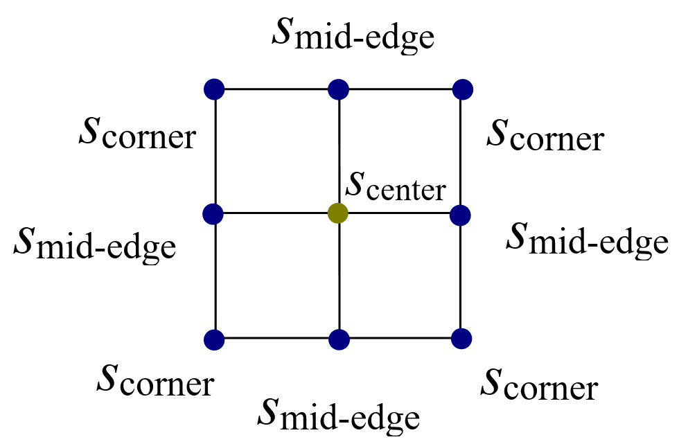
Figure 1: A schematic representation of the FLAME scheme (1) for the 2D Helmholtz equation in free space. Grid size $h$ in both coordinate directions.

$$s_{\mathrm{center}}=\frac{A}{D}\left(e_{\frac{1}{2}}+1\right),~{}~{}s_{\mathrm{mid-edge}}=-\frac{B}{D},~{}~{}s_{\mathrm{corner}}=\frac{C}{D}\,e_{-\frac{1}{2}}$$ (1)

where

$$A~{}=~{}e_{\frac{1}{2}}e_{1}+2e_{\frac{1}{2}}e_{0}-4e_{-\frac{1}{2}}e_{1}+e_{\frac{1}{2}}-4e_{-\frac{1}{2}}+e_{1}+2e_{0}+1$$

$$B~{}=~{}e_{\frac{3}{2}}e_{0}-2e_{\frac{1}{2}}e_{1}+2e_{\frac{1}{2}}e_{0}-2e_{\frac{1}{2}}+e_{0}$$

$$C~{}=~{}2e_{\frac{1}{2}}e_{0}-e_{-\frac{1}{2}}e_{1}-2e_{-\frac{1}{2}}e_{0}-e_{-\frac{1}{2}}+2e_{0}$$

$$D~{}=~{}(e_{0}-1)^{2}(e_{-\frac{1}{2}}-1)^{4};$$

$$e_{\gamma}\,=\,\exp(2^{\gamma}ihk),\quad\gamma\,=\,-\frac{1}{2},0,\frac{1}{2},1,\frac{3}{2}$$

This stencil is schematically represented in Fig. 1.

For (1) and similar schemes, it is not immediately obvious what the “right” scaling should be (whether multiplication by a certain power of $h$ would be appropriate). In a comprehensive convergence theory, which would include stability analysis in addition to approximation errors, the scaling issue would not be critical for the analysis of global errors, but would still matter for the assessment of local ones. In any event, since stability is much more difficult to study than approximation, it is desirable to establish a universal measure by which the local approximation accuracy of difference schemes can be compared in a consistent manner.

Godunov & Ryabenkii (G&R) discuss a closely related but different issue [16, Section 5.13]. They note that consistency error can be formally reduced by changing the norm in which this error is measured. Incorporating an arbitrary power of $h$ into that norm or, even more dramatically, a factor like $2^{-1/h}$, one could magically “improve” the accuracy of the scheme, although the numerical solution would remain unchanged. Given a discrete space $U_{h}$ where an FD scheme “lives” and the corresponding continuous space $U$ for the underlying boundary value problem, G&R write:

It is customary to choose a norm in the space $U_{h}$ in such a way that, as $h$ tends to zero, it will go over into some norm for functions given on the whole [domain], i.e. so that

$$\lim_{h\rightarrow 0}\|u_{h}\|_{U_{h}}\,=\,\|u\|_{U}$$ (2)

Trivial examples of that are (i) the maximum norms in both spaces; (ii) the discrete norm $\|u_{h}\|_{U_{h}}^{2}=\left(h^{d}\sum_{m}|u_{m}|^{2}\right)$, which transforms into the $L_{2}$ norm as $h\rightarrow 0$.

G&R’s condition (2) is natural but separate from the scaling issue. Indeed, even if the norms in both discrete and continuous spaces are fixed (say, for the sake of argument, taken to be the maximum-norms), the scheme can still be rescaled by an arbitrary factor, including an $h$-dependent factor.

To proceed further, we need to recall the Lax-Richtmyer theorem relating consistency, stability and convergence [17, 16]. The connection is easy to see if the difference systems for the numerical and exact solutions are written side by side:

$$S_{h}\underline{u}_{h}\,=\,\underline{f}_{h};\quad S_{h}\underline{u}^{*}_{h}\,=\,\underline{f}_{h}+\underline{\epsilon}_{c}$$

Subtracting these equations, one immediately observes that

$$S_{h}\underline{\epsilon}_{s}\,=\,\underline{\epsilon}_{c},~{}~{}~{}\underline{\epsilon}_{s}\equiv\underline{u}_{h}-\underline{u}^{*}_{h}$$ (3)

or equivalently

$$\underline{\epsilon}_{s}\,=\,S_{h}^{-1}\underline{\epsilon}_{c}$$ (4)

Here $\underline{\epsilon}_{s}\in\mathbb{C}^{n}$ (or $\mathbb{R}^{n}$, depending on the type of the problem) is the solution error vector. This is a simple but critical result relating consistency and solution errors. It is important to note, however, that all the quantities in (4) are global.

III Accuracy of Yee-like Schemes:
General Considerations

We can now take a closer look at the accuracy of Yee-like schemes near slanted material boundaries. Consider an FD scheme in the following generic form, in the absence of sources:

$$\underline{u}^{(i)T}\underline{s}^{(i)}(h,\mathrm{\Delta}t,\epsilon,\mu)\,=\,0$$ (5)

where $\underline{u}^{(i)}$ is a Euclidean vector of degrees of freedom corresponding to a particular grid “molecule” $i$ with node locations $\mathbf{r}_{\beta}^{(i)},t_{\beta}^{(i)}$ ($\beta=1,2,\ldots,n$), and $\underline{s}$ is the coefficient vector defining the scheme. As indicated in (5), these coefficients depend on the electromagnetic parameters $\epsilon=\epsilon(\mathbf{r})$ and $\mu=\mu(\mathbf{r})$ (assuming linear characteristics of all media). It is convenient to introduce a small local domain $\mathrm{\Omega}^{(i)}$ containing the grid molecule (e.g. the convex hull of the nodes of the molecule); diam $\mathrm{\Omega}^{(i)}$ is thus of the order of the grid size.

The local (stencil-wise) consistency error $\epsilon_{c}^{(i)}$ is defined as

$$\epsilon_{c}^{(i)}(h,\mathrm{\Delta}t,\epsilon,\mu)\,=\,\underline{s}^{(i)T}\mathcal{N}^{(i)}u^{*}$$ (6)

In this expression, $\underline{u}^{*}$ could in principle be any vector defined on the grid molecule, but is almost always taken to be the column vector of nodal values of the exact solution $u^{*}$ of the underlying boundary value problem. Formally, therefore, $u^{*}\in\mathcal{T}(\mathrm{\Omega}^{(i)})$, where $\mathcal{T}(\mathrm{\Omega}^{(i)})$ is the local Trefftz space – that is, the space of functions satisfying the underlying weak-form differential equations in $\mathrm{\Omega}^{(i)}$. Finally, the operator $\mathcal{N}^{(i)}:\mathcal{T}(\mathrm{\Omega}^{(i)})\rightarrow\mathbb{R}^{n}$ (or $\mathbb{C}^{n}$) in (4) produces $n$ given degrees of freedom (typically, the nodal values) of any given local solution $u^{*}$.

Our goal is to establish an accuracy measure which, unlike $\epsilon_{c}^{(i)}$ (6), would be independent of the scaling of the scheme $\underline{s}^{(i)}$. Obviously, the numerical solution does not, in the absence of roundoff errors, depend on this scaling. (If all stencils were to be simultaneously rescaled by any nonzero factor $\kappa$, the inverse matrix $S_{h}^{-1}$ in (4) would also be simultaneously rescaled, but by the inverse factor $\kappa^{-1}$.) Although this is in principle clear, theoretical analysis faces several impediments – partly mathematical and partly practical:

1. Rigorous analytical estimates of the stability factor related to the norm of $S^{-1}$ are available for fairly simple model problems but may be difficult or impossible to obtain for more complicated practical ones. It is therefore desirable to find a meaningful way to characterize approximation independently of stability.

2. The Lax-Richtmyer estimate (3) is global and does not connect the local solution errors to the respective local consistency errors. Such local estimates are available for finite element methods, thanks to variational formulations and duality principles [22, 23, 24, 25, 26, 27, 28], but not for FD schemes.

3. To reiterate, stability is, by its nature, a global feature; that is, it pertains to the system of FD equations as a whole. At the same time, local approximation errors are of interest in their own right. In particular, one may wish to compare the local accuracy of two schemes, possibly derived from completely different considerations and involving disparate degrees of freedom.

Two general and scaling-independent ways of examining the local errors are introduced in Sections IV and V below.

IV Trefftz Test Matrix and Its
Minimum Singular Value

Obviously, for any single solution $u^{*}$ one can generate infinitely many exact schemes – that is, schemes with a zero consistency error $\epsilon_{c}$ (6). Since only one FD stencil is considered in the remainder of this section, the superscript $(i)$ indicating the stencil number is now dropped. Let the position vectors of $n$ stencil nodes be $\mathbf{r}_{\beta}$, $\beta=1,2,,\ldots,n$.

Suppose that we have a Trefftz test set of $m$ different solutions $u^{*}_{1,\ldots,m}(\mathbf{r})$ independent of the mesh size and time step. By definition, Trefftz functions – in particular, $u^{*}_{\alpha}(\mathbf{r})$ – satisfy the differential equation of the problem and interface boundary conditions (if any) within the convex hull of the grid molecule. We want the consistency error to be small for each test solution.

Let us arrange the nodal values of $u^{*}_{1,\ldots,m}(\mathbf{r})$ in a matrix $U$: each row $\alpha$ of $U$ contains the nodal values of the test solution $u^{*}_{\alpha}(\mathbf{r})$, so that

$$U_{\alpha\beta}~{}=~{}u^{*}_{\alpha}(\mathbf{r}_{\beta})$$ (7)

Assembling the consistency errors (6) for all test solutions into one Euclidean vector $\underline{\epsilon}_{c}\in\mathbb{R}^{m}$, we get

$$\underline{\epsilon}_{c}\,\equiv\,U\underline{s}\quad~{}~{}\Rightarrow\quad~{}~{}\|\underline{\epsilon}_{c}\|_{2}\,\geq\,\sigma_{\min}(U)\|\underline{s}\|_{2}$$ (8)

where $\sigma_{\min}(U)$ is the minimum singular value of $U=U(h,\mathrm{\Delta}t,\epsilon,\mu)$. This is a lower bound of the consistency error. Using different sets of Trefftz functions, or one large set, one can obtain different bounds of this form.

A rigorous mathematical solution of the stability and scaling problems is not in general available, but the error bound (8) suggests an alternative on physical/engineering grounds. Namely, one can compare the minimum singular values of matrix $U(h,\mathrm{\Delta}t,\epsilon,\mu)$ and its free-space instantiation $U_{1}(h,\mathrm{\Delta}t)=U(h,\mathrm{\Delta}t,\epsilon=1,\mu=1)$:

$$\zeta\,=\,\frac{\sigma_{\min}(U(h,\mathrm{\Delta}t,\epsilon,\mu))}{\sigma_{\min}(U(h,\mathrm{\Delta}t,1,1))}$$ (9)

Clearly, in the inhomogeneous case one may expect the estimate (8) to be worse than the respective one for free space; hence typically $\zeta>1$ and quite possibly $\zeta\gg 1$. Let us consider illustrative examples.

Example 1

To start with, we calculate just the free-space value $\sigma_{\min}(U_{1})$ for the 2D Laplace equation $\nabla^{2}u=0$. Introduce the standard five-point stencil and assume, for simplicity of notation, the same grid size $h$ in both coordinate directions; the node coordinates are

$$x_{1,\ldots,5}=\{0,0,-h,h,0\};~{}~{}~{}y_{1,\ldots,5}=\{0,-h,0,0,h\}$$

(thus, node #1 is the central node in this grid molecule). Let the Trefftz basis $\{u^{*}_{\alpha}(x,y)\}$ consist of harmonic polynomials up to order 4 (these are the real and imaginary parts of $(x+iy)^{k},k=0,\ldots,4$):

$$u^{*}_{1,\ldots,8}=\{1,x,y,x^{2}-y^{2},2xy,x^{3}-3xy^{2},3x^{2}y-y^{3},x^{4}-6x^{2}y^{2}+y^{4}\}$$

Then the $U$ matrix is

$$U=\begin{pmatrix}1~{}&~{}0~{}&~{}0~{}&~{}0~{}&~{}0~{}&~{}0~{}&~{}0~{}&~{}0\\ 1~{}&~{}0~{}&~{}-h~{}&~{}-h^{2}~{}&~{}0~{}&~{}0~{}&~{}h^{3}~{}&~{}h^{4}\\ 1~{}&~{}-h~{}&~{}0~{}&~{}h^{2}~{}&~{}0~{}&~{}-h^{3}~{}&~{}0~{}&~{}h^{4}\\ 1~{}&~{}h~{}&~{}0~{}&~{}h^{2}~{}&~{}0~{}&~{}h^{3}~{}&~{}0~{}&~{}h^{4}\\ 1~{}&~{}0~{}&~{}h~{}&~{}-h^{2}~{}&~{}0~{}&~{}0~{}&~{}-h^{3}~{}&~{}h^{4}\end{pmatrix}$$

(Recall that each column of this matrix contains the nodal values of the respective test function. Obviously, function $2xy$, corresponding to the zero column, could have been omitted from the basis.)

Symbolic algebra gives the following lowest order terms for the singular values of $U$:

$$\sigma_{1,\ldots,5}(N)\sim\{2h^{2},\,2^{\frac{1}{2}}h,\,2^{\frac{1}{2}}h,\,2\cdot 5^{-\frac{1}{2}}h^{4},\,5^{\frac{1}{2}}\}$$

Hence

$$\sigma_{\min}(U)\overset{h\ll 1}{=}\sigma_{4}(U)\sim 2\cdot 5^{-\frac{1}{2}}h^{4}=\mathcal{O}(h^{4})$$

Example 2

Consider now the 2D wave equation

$$v^{2}\nabla^{2}u-\partial_{t}^{2}u=0$$

We follow the same exact steps as in the previous example.

The simplest grid “molecule” has seven nodes in the $xyt$ space:

$$x_{1,\ldots,7}=\{0,0,-h,h,0,0,0\}$$

$$y_{1,\ldots,7}=\{0,-h,0,0,h,0,0\}$$

$$t_{1,\ldots,7}=\{0,0,0,0,0,-\mathrm{\Delta}t,\mathrm{\Delta}t\};$$

where the Trefftz test set $\{u_{\alpha}(x,y)\}$ is now chosen as

$$u^{*}_{1,\ldots,17}=\{1,(x\pm vt)^{k},(y\pm vt)^{k}\},~{}~{}~{}k=1,2,3,4$$ (10)

For the $U$ matrix corresponding to the chosen grid molecule and test set (10), symbolic algebra yields

$$\sigma_{\min}(U)\overset{h\ll 1}{\sim}c_{4}h^{4}$$ (11)

The analytical expression for the coefficient $c_{4}$ is too cumbersome to be reproduced here, but it is plotted, as a function of $v\mathrm{\Delta}t/h$, in Fig. 2.

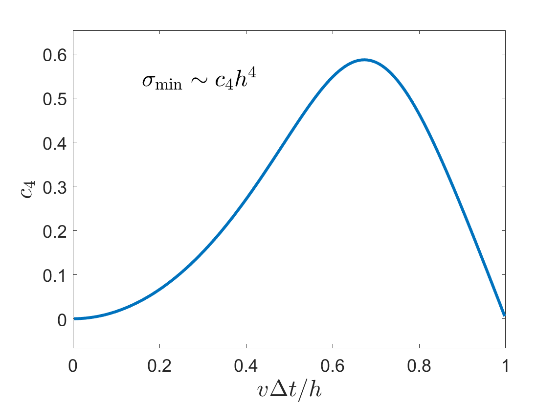
Figure 2: Coefficient $c_{4}$ of (11) vs. $v\mathrm{\Delta}t/h$, where $\sigma_{\min}(U)\sim c_{4}h^{4}$.

Example 3

Following the preliminary examples above, we are in a position to examine the Yee setup in 2D in a similar fashion. Consider two dielectric media with permittivities $\epsilon_{1,2}$, separated by a slanted interface boundary (Fig. 3). Of most interest is the $H$-mode ($p$-mode), with a one-component $\mathbf{H}$ field perpendicular to the plane of the figure and a two-component $\mathbf{E}$ field whose normal component is discontinuous across the interface. The $H$ nodes are labeled with the yellow spheres in the figure, and the $E_{x,y}$ components – with the arrows. The time axis is for simplicity not shown, but it is understood that the central $H$ sphere indicates in fact a triple Yee node ($t_{0},t_{0}\pm\mathrm{\Delta}t$), and that the $E_{x,y}$ arrows indicate double nodes ($t_{0}\pm\mathrm{\Delta}t/2$); $t_{0}$ is any “current” moment of time. There are 7 degrees of freedom for the $H$ field (five at $t_{0}$ and two at $t_{0}\pm\mathrm{\Delta}/2$) and $2\times 4=8$ for $E_{x,y}$ – altogether 15 degrees of freedom.

One horizontal and one vertical black lines in Fig. 3 belong to the $H$ grid with a size $h$ in each direction; the finer blue grid indicates $h/4$ subdivisions as a visual aid. The slope $\theta$ of the interface is an adjustable parameter. For definiteness, we take $\theta=30^{\circ}$ and assume that the interface boundary divides the “horizontal” segment between two adjacent $H$ nodes in the ratio of 1:3, as indicated in the figure. With this geometric setup, two $H$ nodes (the left one and the top one) happen to lie in the $\epsilon_{1}$ dielectric, as does the top “double node” $E_{x}$. All other nodes lie in the second dielectric.

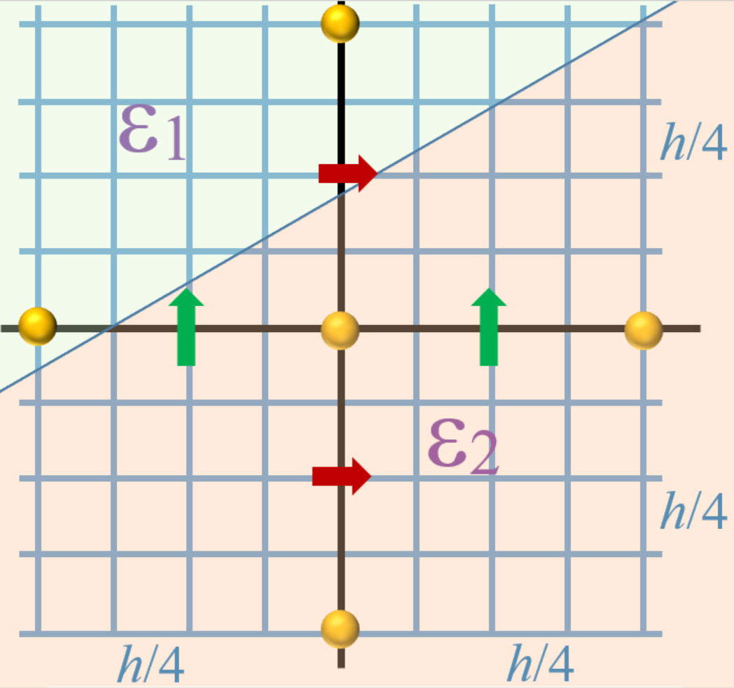
Figure 3: Yee-like schemes near material boundaries. $H$-mode ($p$-mode): a one-component $\mathbf{H}$ field perpendicular to the plane of the figure and a two-component $\mathbf{E}$ field in the plane. Two dielectric media ($\epsilon_{1,2}$) with an interface boundary slanted with respect to the Yee grid. Yellow spheres: $H$ nodes; horizontal arrows: $E_{x}$ nodes; vertical arrows: $E_{y}$ nodes. The central $H$ sphere indicates a triple node with respect to time ($t_{0},t_{0}\pm\mathrm{\Delta}t$), and the $E_{x,y}$ arrows indicate double nodes ($t_{0}\pm\mathrm{\Delta}t/2$); $t_{0}$ is any “current” moment of time.

The Trefftz test set is a slightly generalized version of (10). Now that two media with their respective phase velocities $v_{1,2}$ are present, each polynomial of the form $(x\pm v_{1}t)^{k}$, $(y\pm v_{1}t)^{k}$ in the first subdomain is matched, via the standard interface boundary conditions, with the corresponding polynomial $(x\pm v_{2}t)^{k}$, $(y\pm v_{2}t)^{k}$ in the second subdomain; we take $k=0,1,2,3$.

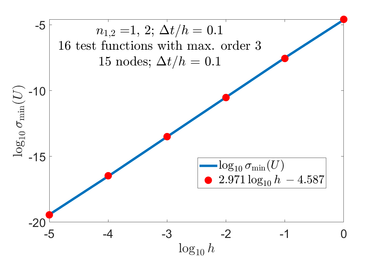
Figure 4: $\log_{10}\sigma_{\min}(N)$ vs. $\log_{10}h$. Solid line: $\log_{10}\sigma_{\min}(U)$; markers: linear fit with slope K$\approx 3$. Indexes of refraction $n_{1,2}=$1, 2. $c\mathrm{\Delta}t/h=$ 0.1. Geometric setup of p. 3; material interface at angle $\theta=\pi/$6. 15-node stencil: 7 nodes for $H$, $2\times 2=4$ nodes for $E_{x}$, $2\times 2=4$ nodes for $E_{y}$. Trefftz test basis: polynomial traveling waves in each dielectric, matched via the standard interface boundary conditions (see text).

The rest of the analysis proceeds the same way as in the previous examples, except that a final closed-form analytical result for $\sigma_{\min}(U)$, where $U$ is in this case a $15\times 16$ matrix, is no longer feasible to obtain via symbolic algebra. Instead, this smallest singular value is computed in variable precision arithmetic (32 digits). The results are plotted in Fig. 4 and clearly indicate that

$$\sigma_{\min}(U)\,=\,\mathcal{O}(h^{3})\quad\left(\mathrm{fixed}~{}\frac{c\mathrm{\Delta}t}{h}\right)$$ (12)

At the same time, in free space

$$\sigma_{\min}(U)\,=\,\mathcal{O}(h^{4})\quad\left(\mathrm{fixed}~{}\frac{c\mathrm{\Delta}t}{h}\right)$$ (13)

That is, in the presence of a dielectric interface one cannot achieve the same order of convergence of Yee-like schemes as in free space, and the deterioration factor $\zeta$ (9) is

$$\zeta_{\mathrm{Yee}}\,=\,\mathcal{O}\left(h^{-3}/h^{-4}\right)\,=\,\mathcal{O}(h)$$ (14)

This conclusion is not entirely unexpected. Its limitation is that this analysis has been applied to specific degrees of freedom adopted in classical Yee schemes – that is, the nodal values of the fields on staggered grids. A generalization to other degrees of freedom – notably, to edge circulations and/or surface fluxes – and to non-staggered grids is certainly possible. However, the odds of preserving the second order of the free-space Yee scheme in the presence of interfaces are slim; see also [30]. On the positive side, as already noted, second-order schemes are available for interface boundaries parallel to the gridlines, and there is also compelling evidence that global quantities can also be evaluated with second-order accuracy if FDTD schemes are constructed judiciously [8, 5].

V Approximation in Trefftz Subspaces

Recall that consistency error, by its standard definition (6), depends on the scaling of the underlying scheme. Namely, multiplication of the scheme by an arbitrary factor, including a factor depending on the grid size $h$ and/or the time step $\mathrm{\Delta}t$, leads to a commensurate change of the consistency error. A related observation is that FEM on regular grids often produces essentially the same schemes as standard FD, except for an extra factor of the order $\mathcal{O}(h^{d})$ due to integration ($d=1,2,3$ is the number of dimensions). Finally, schemes like FIT, where degrees of freedom are field circulations and fluxes rather than nodal values, also involve inherently different scaling factors.

Notably, in finite element analysis the focus is on continuous-level approximation rather than FD-type consistency errors. Arguably, the former is more fundamental than the latter – in particular, continuous-level errors do not depend on any scaling of the respective FE equations. More precisely, given a finite element $K$, a suitable functional space $X=X(K)$, a function $u\in X(K)$ and, importantly, a finite-dimensional subspace $X_{h}=X_{h}(K)\subset X(K)$, the approximation error for $u$ is unambiguously defined as

$$\epsilon_{a}\,\overset{\mathrm{def}}{=}\inf_{u_{h}\in X_{h}}\|u-u_{h}\|$$ (15)

With this definition, the error is completely decoupled from any algebraic manipulation of the FE system of equations. (As an example, one may consider a triangular element $K$ and choose: $X(K)=H^{2}(K)$, $X_{h}(K)$ – the space of linear functions over $K$, and either $H^{1}$ or $L_{2}$ norms in (15); the standard FE approximation error estimates ensue [31, 32].)

This serves as a motivation to look for an analogous error measure in the FD context. It should be emphasized from the outset that this measure is local – that is, it applies to a single FD grid molecule.

Consider an $N$-dimensional Trefftz space $\mathcal{T}_{N}(\mathrm{\Omega}^{(i)})$ ($N\gg 1$) corresponding to a given weak-form differential equation over a (small) domain $\mathrm{\Omega}^{(i)}$ covering a particular grid molecule. Equipped with a suitable inner product $[\cdot\,,\cdot]$ and the respective norm, $\mathcal{T}_{N}(\mathrm{\Omega}^{(i)})$ is a Hilbert space. A natural choice of such inner product would be the standard one of $L_{2}$ or $H^{1}$, but scaled by a factor $\mathcal{O}(h^{-d})$ in $d=1,2,3$ dimensions, to compensate for the smallness of the volume of $\mathrm{\Omega}^{(i)}$.

A given FD stencil (i.e. a set of coefficients – for definiteness, real-valued) $\underline{s}^{(i)}\in\mathbb{R}^{n}$ can be viewed as a linear functional $g:~{}\mathcal{T}_{N}(\mathrm{\Omega}^{(i)})\rightarrow\mathbb{R}$. We focus on the case where $\mathrm{\Omega}^{(i)}$ is source-free, so the right hand side of the underlying differential equation and the FD scheme is zero.

A key idea is to introduce the “Trefftz” subspace $T_{h}(\mathrm{\Omega}^{(i)})\subset\mathcal{T}_{N}(\mathrm{\Omega}^{(i)})$ of functions satisfying the FD scheme exactly; that is,

$$\mathcal{T}_{h}(\mathrm{\Omega}^{(i)}):~{}~{}\{u\in\mathcal{T}_{N}(\mathrm{\Omega}^{(i)}),~{}~{}\langle g,u\rangle\,=\,0\}$$ (16)

We shall refer to $\mathcal{T}_{h}$ by the acronym SETS: scheme-exact Trefftz subspace. By the Riesz representation theorem, the linear functional $g$ can be written as

$$\langle g,\,u(\mathbf{r})\rangle\,=\,[g_{\bot}(\mathbf{r}),\,u(\mathbf{r})],\quad\forall u\in\mathcal{T}_{N}(\mathrm{\Omega}^{(i)})$$ (17)

for some $g_{\bot}(\mathbf{r})\in\mathcal{T}_{N}(\mathrm{\Omega}^{(i)})$. Dependence on the position vector $\mathbf{r}$ is explicitly shown to distinguish functions in $\mathcal{T}_{N}$ from vectors or functionals. With this notation at hand, the SETS $\mathcal{T}_{h}$ can be written as

$$\mathcal{T}_{h}(\mathrm{\Omega}^{(i)}):~{}~{}\{u(\mathbf{r})\in\mathcal{T}_{N}(\mathrm{\Omega}^{(i)}),~{}~{}[g_{\bot}(\mathbf{r}),u(\mathbf{r})]\,=\,0\}$$ (18)

For any given $u(\mathbf{r})\in\mathcal{T}_{N}(\mathrm{\Omega}^{(i)})$, one can then define the approximation error

$$\epsilon_{a}\,=\,\inf_{u_{h}\in\mathcal{T}_{h}(\mathrm{\Omega}^{(i)})}\|u-u_{h}\|_{\mathcal{T}_{h}(\mathrm{\Omega}^{(i)})}$$ (19)

A critical observation is that the subspace $\mathcal{T}_{h}$ does not depend on the scaling of the FD scheme, and hence the approximation error (19) does not either, in contrast with the standard consistency error $\epsilon_{c}$. The approximation error $\epsilon_{a}$ is determined by solving an orthogonal projection problem; one obtains

$$\epsilon_{a}\,=\,\frac{\left|\,[u(\mathbf{r}),\,g_{\bot}(\mathbf{r})]\,\right|}{\|g_{\bot}(\mathbf{r})\|_{\mathcal{T}_{N}}}$$ (20)

An explicit expression for $g_{\bot}(\mathbf{r})$ can be found if a basis in $\mathcal{T}_{N}$ is introduced (see Appendix).

Example 4

For illustration, let us consider one relatively simple example: the 2D Laplace equation $\nabla^{2}u=0$ and the five- and nine-point stencils shown in Fig. 5. (The former is standard, and the latter can be viewed as either a Mehrstellen or FLAME scheme [33].)

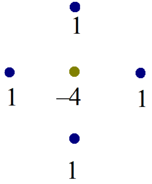
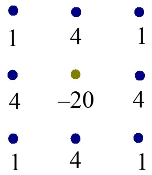
Figure 5: Standard five-point and nine-point stencils for the 2D Laplace equation.

The above procedure for evaluating the approximation error was implemented in symbolic algebra for the following setup:

• The Trefftz basis set of $N=2m+1$ harmonic polynomials $\underline{\psi}=\{1,\mathrm{Re}\,z^{m}$, $\mathrm{Im}\,z^{m}\}$, $m=1,2,\ldots,M$, $z=x+iy$.

• The Trefftz space $\mathcal{T}_{N}=\mathrm{span}\,\underline{\psi}$, equipped with the inner product $(2h)^{-2}(\cdot\,,\,\cdot)_{L_{2}}$ and the respective norm. The factor $(2h)^{-2}$ compensates for the smallness of the area of the subdomain $\mathrm{\Omega}^{(i)}=[-h,h]\times[-h,h]$.

Typical results for the basis set of harmonic polynomials of orders up to $M=10$ are summarized in Table I.

TABLE I: The lead terms in Trefftz-space approximation errors for the 5-point and 9-point stencils; the 2D Laplace equation.

	$h^{-2}\|\cdot\|_{L_{2}}$	$h^{-2}\|\cdot\|_{H^{1}}$	$h^{-2}\|\cdot\|_{H^{2}}$
5-point stencil	$\sim 0.655h^{4}$	$\sim 4.17h^{3}$	$\sim 12.6h^{2}$
9-point stencil	$\sim 1.99h^{8}$	$\sim 18.5h^{7}$	$\sim 98.5h^{6}$

Explicitly, for the standard 5-point scheme (Fig. 5, left) and $M=4$, one obtains

$$g_{\bot}(\mathbf{r})\,=\,-\frac{1575(x^{4}-6x^{2}y^{2}+y^{4})}{208h^{4}}-\frac{105}{52};$$

$$\|g_{\bot}(\mathbf{r})\|\,=\,\frac{15\sqrt{91}}{26}$$

For the following test function as an example

$$f_{\mathrm{test}}=\exp 2x\cos 2y\quad\quad(\nabla^{2}f_{\mathrm{test}}=0)$$

the approximation error (20) is calculated to be

$$\epsilon_{a}\,=\,\frac{16\sqrt{91}}{315}\,h^{4}\,+\,\mathrm{higher~{}order~{}terms}$$

Repeating this symbolic algebra analysis for the 9-point scheme (Fig. 5, right) and $M=8$, we get $\|g_{\bot}(\mathbf{r})\|_{L_{2}}=10725\cdot 665270333^{\frac{1}{2}}/3440312\approx 80.4$. (The actual expression for $g_{\bot}(\mathbf{r})$ itself is too cumbersome to be worth reproducing here.) For the same test function $f_{\mathrm{test}}$ as before,

$$\epsilon_{a}\,=\,\frac{256\sqrt{665270333}}{1045269225}\,h^{8}\,+\,\mathrm{higher~{}order~{}terms}$$

In all cases the approximation error (20) is independent of the scaling of the scheme; to verify that experimentally, the schemes of Fig. 5 were multiplied with arbitrary factors, and the symbolic algebra results for the error remained unchanged. Naturally, though, the approximation accuracy does depend on the choice of the norm in the Trefftz space $\mathcal{T}_{N}$.

VI Conclusion

This paper addresses several accuracy-related issues which, despite their principal theoretical and practical importance for FD schemes in electromagnetic applications, have been overlooked and/or remain controversial. An important example is the order of Yee-like schemes in the vicinity of slanted or curved material interfaces: in the existing literature conflicting claims have been made as to whether this order can be higher than one. This inconsistency is due to several factors: (i) difference in the accuracy of local and global quantities for FD solutions; (ii) a very large variety of techniques proposed for accuracy improvement, and complexity of their mathematical analysis; (iii) the dependence of the consistency error on the scaling of the scheme (Section II).

The paper focuses on local consistency errors and puts forward two practical methods for an “apples vs. apples” comparison of various difference schemes with arbitrary degrees of freedom, in homogeneous regions and especially in the presence of material interfaces. The first method makes use of Trefftz test matrices (Section IV), while the second one relies on a new measure of approximation accuracy in scheme-exact Trefftz subspaces introduced in Section V. One particular conclusion is that a loss of local approximation accuracy by one order is unavoidable for Yee-like schemes at slanted material boundaries.

Appendix: An Expression for $g_{\bot}$

Let $\underline{\psi}(\mathbf{r})=\{\psi_{\alpha}(\mathbf{r})\}$ be a basis in $\mathcal{T}_{N}$, arranged as a column vector. Then any function $u(\mathbf{r})\in\mathcal{T}_{N}$ can be expanded as

$$u(\mathbf{r})\,=\,\underline{u}^{T}\underline{\psi}(\mathbf{r}),\quad\underline{u}\in\mathbb{R}^{N}$$ (21)

where the column vectors are underlined. Euclidean inner product and that of $\mathcal{T}_{N}$ are related as

$$[u(\mathbf{r}),v(\mathbf{r})]\,=\,[\underline{u}^{T}\underline{\psi}(\mathbf{r}),\,\underline{v}^{T}\underline{\psi}(\mathbf{r})]\,=\,(\mathrm{\Psi}\underline{u}\,,\,\underline{v})$$ (22)

Here $\mathrm{\Psi}$ is the Gram matrix of the basis functions:

$$\mathrm{\Psi}\,=\,[\underline{\psi},\,\underline{\psi}^{T}]\quad\Longleftrightarrow\quad\mathrm{\Psi}_{\alpha\beta}=[\psi_{\alpha}\,,\,\psi_{\beta}],~{}~{}1\leq\alpha,\beta\leq N$$ (23)

Applying the $g$ functional – that is, the difference scheme – to each of the basis functions, one obtains the column vector

$$\underline{g}_{\psi}\,=\,\langle g\,,\,\underline{\psi}(\mathbf{r})\rangle\,\in\,\mathbb{R}^{N}$$ (24)

We can now determine the vector $g_{\bot}(\mathbf{r})$ representing in $\mathcal{T}_{N}$ the functional $g$ and hence the difference scheme itself. We have

$$\langle g\,,\,u(\mathbf{r})\rangle\,\overset{\eqref{eqn:linear-functional-eq-xi-u}}{=}\,[g_{\bot}(\mathbf{r}),u(\mathbf{r})]\,\overset{\eqref{eqn:inner-prods-T-RN}}{=}\,(\mathrm{\Psi}\underline{g},\,\underline{u})$$ (25)

Setting in this equation $u(\mathbf{r})=\psi_{\alpha}(\mathbf{r})$, the respective $\underline{u}$ being the unit vector $e_{\alpha}$, we derive

$$\underline{g}_{\psi\alpha}\equiv\langle g,\,\psi_{\alpha}(\mathbf{r})\rangle\,=\,(\mathrm{\Psi}\underline{g}\,,\,e_{\alpha})\,=\,(\mathrm{\Psi}\underline{g})_{\alpha}$$ (26)

This gives an explicit expression for $\underline{g}$ – that is, for the representation of $g_{\bot}(\mathbf{r})$ (20) in the $\{\psi\}$ basis:

$$\underline{g}\,=\,\mathrm{\Psi}^{-1}\underline{g}_{\psi}$$ (27)

As a reminder, $\underline{g}$ in the left hand side is the column vector corresponding in the chosen $\underline{\psi}$ basis to $g_{\bot}(\mathbf{r})$, while the column vector $\underline{g}_{\psi}$ (24) contains the values of the difference scheme evaluated on each basis function.

For any function $u(\mathbf{r})\in\mathcal{T}_{N}$, its orthogonal projection onto the SETS $\mathcal{T}_{h}$ has the form

$$u_{h}(\mathbf{r})\,=\,u(\mathbf{r})-\alpha g_{\bot}(\mathbf{r})$$ (28)

where the coefficient $\alpha$ is found from the orthogonality condition

$$[u(\mathbf{r})-\alpha g_{\bot}(\mathbf{r}),\,g_{\bot}(\mathbf{r})]\,=\,0$$ (29)

so that

$$\alpha\,=\,\frac{[u(\mathbf{r}),\,g_{\bot}(\mathbf{r})]}{[g_{\bot}(\mathbf{r}),\,g_{\bot}(\mathbf{r})]}\,=\,\frac{(\Psi\underline{u}\,,\,\underline{g})}{(\Psi\underline{g},\,\underline{g})}$$ (30)

References

- [1] V. Thomée, “From finite differences to finite elements: A short history of numerical analysis of partial differential equations,” J. of Comp. and Applied Math., vol. 128, pp. 1–54, 2001.
- [2] K. S. Yee, “Numerical solution of initial boundary value problems involving Maxwell’s equations in isotropic media,” IEEE Trans. Antennas & Prop., vol. AP-14, no. 3, pp. 302–307, 1966.
- [3] T. Hirono, Y. Shibata, W. W. Lui, S. Seki, and Y. Yoshikuni, “The second-order condition for the dielectric interface orthogonal to the Yee-lattice axis in the FDTD scheme,” IEEE Microw & Guided Wave Lett, vol. 10, no. 9, pp. 359–361, 2000.
- [4] K.-P. Hwang and A. C. Cangellaris, “Effective permittivities for second-order accurate FDTD equations at dielectric interfaces,” IEEE Microw & Wireless Compon Lett, vol. 11, no. 4, pp. 158–160, April 2001.
- [5] D. M. Shyroki, “Modeling of sloped interfaces on a Yee grid,” IEEE Trans Ant Propag, vol. 59, no. 9, pp. 3290–3295, 2011.
- [6] A. Farjadpour, D. Roundy, A. Rodriguez, M. Ibanescu, P. Bermel, J. D. Joannopoulos, S. G. Johnson, and G. W. Burr, “Improving accuracy by subpixel smoothing in the finite-difference time domain,” Opt Lett, vol. 31, no. 20, pp. 2972–2974, 2006.
- [7] A. F. Oskooi, C. Kottke, and S. G. Johnson, “Accurate finite-difference time-domain simulation of anisotropic media by subpixel smoothing,” Opt. Lett., vol. 34, no. 18, pp. 2778–2780, Sep 2009.
- [8] C. A. Bauer, G. R. Werner, and J. R. Cary, “A second-order 3d electromagnetics algorithm for curved interfaces between anisotropic dielectrics on a Yee mesh,” J Comp Phys, vol. 230, no. 5, pp. 2060–2075, 2011.
- [9] M. Clemens and T. Weiland, “Magnetic field simulation using conformal FIT formulations,” IEEE Trans. Magn., vol. 38, no. 2, pp. 389–392, 2002.
- [10] I. Tsukerman, “Electromagnetic applications of a new finite-difference calculus,” IEEE Trans. Magn., vol. 41, no. 7, pp. 2206–2225, 2005.
- [11] ——, “A class of difference schemes with flexible local approximation,” J. Comput. Phys., vol. 211, no. 2, pp. 659–699, 2006.
- [12] I. Tsukerman and F. Čajko, “Photonic band structure computation using FLAME,” IEEE Trans Magn, vol. 44, no. 6, pp. 1382–1385, 2008.
- [13] F. Čajko and I. Tsukerman, “Flexible approximation schemes for wave refraction in negative index materials,” IEEE Trans. Magn., vol. 44, no. 6, pp. 1378–1381, 2008.
- [14] I. Tsukerman, “Trefftz difference schemes on irregular stencils,” J of Comput Phys, vol. 229, no. 8, pp. 2948–2963, 2010.
- [15] I. Babuška, F. Ihlenburg, E. T. Paik, and S. A. Sauter, “A generalized finite element method for solving the Helmholtz equation in two dimensions with minimal pollution,” Comput Meth Appl Mech & Eng, vol. 128, pp. 325–359, 1995.
- [16] S. Godunov and V. Ryabenkii, Difference Schemes: an Introduction to the Underlying Theory. Amsterdam; New York: Elsevier Science Pub. Co., 1987.
- [17] J. Strikwerda, Finite Difference Schemes and Partial Differential Equations. Society for Industrial and Applied Mathematics, 2004.
- [18] M. Schauer, P. Hammes, P. Thoma, and T. Weiland, “Nonlinear update scheme for partially filled cells,” IEEE Trans Magn, vol. 39, no. 3, pp. 1421–1423, May 2003.
- [19] H. De Gersem, R. Schuhmann, S. Feigh, and T. Weiland, “Hierarchical FIT/FE discretization for dielectric subcell interfaces,” IEEE Trans Magn, vol. 44, no. 6, pp. 706–709, 2008.
- [20] I. Zagorodnov, R. Schuhmann, and T. Weiland, “A uniformly stable conformal FDTD-method in Cartesian grids,” Int. J. Numer. Model., vol. 16, pp. 127–141, 2003.
- [21] H. Pinheiro and J. P. Webb, “A flame molecule for 3-d electromagnetic scattering,” IEEE Transactions on Magnetics, vol. 45, no. 3, pp. 1120–1123, March 2009.
- [22] A. H. Schatz and L. B. Wahlbin, “Interior maximum norm estimates for finite-element methods,” Mathematics of Computation, vol. 31, no. 138, pp. 414–442, 1977.
- [23] ——, “Maximum norm estimates in the finite-element method on plane polygonal domains .1,” Mathematics of Computation, vol. 32, no. 141, pp. 73–109, 1978.
- [24] ——, “Maximum norm estimates in the finite-element method on plane polygonal domains .2. refinements,” Mathematics of Computation, vol. 33, no. 146, pp. 465–492, 1979.
- [25] ——, “Interior Maximum-Norm Estimates for Finite-Element Methods .2.” Mathematics of Computation, vol. 64, no. 211, pp. 907–928, Jul 1995.
- [26] A. H. Schatz, V. Thomee, and L. B. Wahlbin, “Stability, analyticity, and almost best approximation in maximum norm for parabolic finite element equations,” Communications on Pure and Applied Mathematics, vol. 51, no. 11–12, pp. 1349–1385, Nov–Dec 1998.
- [27] A. Demlow, “Sharply localized pointwise and W-infinity(-1) estimates for finite element methods for quasilinear problems,” Mathematics of Computation, vol. 76, no. 260, pp. 1725–1741, 2007.
- [28] A. Demlow, D. Leykekhman, A. H. Schatz, and L. B. Wahlbin, “Best approximation property in the W-infinity(1) norm for finite element methods on graded meshes,” Mathematics of Computation, vol. 81, no. 278, pp. 743–764, Apr 2012.
- [29] Q. Liu, “The PSTD algorithm: A time-domain method requiring only two cells per wavelength,” Microwave and Optical Technology Letters, vol. 15, no. 3, pp. 158–165, 1997.
- [30] A.-K. Tornberg and B. Engquist, “Consistent boundary conditions for the Yee scheme,” J Comp Phys, vol. 227, no. 14, pp. 6922–6943, 2008.
- [31] P. G. Ciarlet and P.-A. Raviart, “General Lagrange and Hermite interpolation in with applications to finite element methods,” Arch. Rational Mech. Anal., vol. 46, pp. 177–199, 1972.
- [32] P. G. Ciarlet, The Finite Element Method for Elliptic Problems. Amsterdam; New York: North-Holland Pub. Co., 1980.
- [33] I. Tsukerman, Computational Methods for Nanoscale Applications: Particles, Plasmons and Waves. Springer, 2007.