Numerical Solution of Dynamic Portfolio Optimization with Transaction Costs

Abstract

We apply numerical dynamic programming techniques to solve discrete-time multi-asset dynamic portfolio optimization problems with proportional transaction costs and shorting/borrowing constraints. Examples include problems with multiple assets, and many trading periods in a finite horizon problem. We also solve dynamic stochastic problems, with a portfolio including one risk-free asset, an option, and its underlying risky asset, under the existence of transaction costs and constraints. These examples show that it is now tractable to solve such problems.
Keywords: Numerical dynamic programming, dynamic portfolio optimization, transaction cost, no-trade region, option hedging, Epstein-Zin preferences
JEL Classification: C61, C63, G11

1 Introduction

Dynamic management of portfolios is a critical part of any investment strategy by individuals and firms. Multi-stage portfolio optimization problems assume that there are $k$ risky assets and/or a risk-less asset (“bank account” paying a fixed interest rate) traded during a time horizon $[0,T]$, and portfolio adjustments are made at $N$ fixed times in the interval $[0,T]$. Trades are made to maximize the investor’s expected utility over terminal wealth ($T$ is the terminal time) and/or consumption during $[0,T]$.

Standard theory assumes that there is no cost to rebalancing a portfolio, but transaction costs are not negligible in real markets. Not only are there transaction fees such as brokerage expenses, but also the presence of a bid-ask spread creates a transaction cost for a trader. In the modern U.S. stock market, the bid-ask spread is becoming smaller and smaller, but varies across stock prices. If stock prices are high, then the spread could be less than 0.01%, but if stock prices are low, then the spread could be more than 0.1%. Moreover, if risky assets for trading are not stocks, then they may have high transaction costs. For example, if an investor wants to exchange two currencies such as USD and CNY, then transaction costs could be more than 1%. Furthermore, if some risky assets such as housing are not very liquid, then transaction costs could be even higher.

In standard finance theory, the pricing of an option is dependent on the assumptions that its underlying risky asset can be traded at any continuous time without transaction costs and there are no constraints in shorting or borrowing, so that the option can be replicated by the underlying risky asset and one safe asset. However, while the transaction costs may be small in one-time trading, the frequency of rebalancing is theoretically high, so the total transaction cost will be high. Moreover, investors face constraints in shorting risky assets or borrowing cash: they have limits on trading amounts, they have to pay higher costs for shorting risky assets, and they have to pay higher interest rates for borrowing cash than what they receive from saving the same amount of cash in a bank account. Therefore, any examination of real-world dynamic portfolio management needs to consider these frictions/constraints.

In this paper, we first examine multi-stage portfolio optimization problems with proportional transaction costs but no options. If the major transaction cost is the bid-ask spread, then a proportional transaction cost is the correct case to study. For simplicity, we assume that neither shorting risky assets nor borrowing cash is allowed . In fact, if we assume that non-positive wealth has negative infinite utility (i.e., power utility) and the logarithm of returns of risky assets have infinite support in both the low and high end, then the no-shorting and no-borrowing constraints will hold automatically in discrete-time analysis. We also solve these problems with stochastic parameters.

However, in many cases, investors would like to reduce or control the risk and amount of loss in investment strategies. One way is to add put options into the set of portfolio assets as a hedging strategy. A put option is a financial contract that gives its holder the right to sell a certain amount of an underlying asset at a specified price (strike price) within a specified time (time to maturity, or expiration time). Investors may also want to include call options in their portfolio. A call option is a financial contract that gives its holder the right to buy a certain amount of an underlying asset at a specified price (strike price) within a specified time (expiration time). In this paper, we always assume that the options are of European type, that is, the options can only be exercised at the expiration time (but they can still be traded before the expiration time).

Multi-stage portfolio optimization problems with transaction costs have been studied in many papers. The problem with one risky asset has been well studied; see, e.g., Zabel (1973), Constantinides (1976, 1986), Gennotte and Jung (1994), and Boyle and Lin (1997). The key insight is that transaction costs create a “no-trade region” (NTR); that is, no trading is done if the current portfolio is inside the no-trade region, otherwise the investor trades to some point on the boundary of the no-trade region. Kamin (1975) considers the case with only two risky assets. Constantinides (1979) and Abrams and Karmarkar (1980) establish some properties of the NTR for multiple assets, but only present numerical examples with one safe and one risky asset. Brown and Smith (2011) evaluate some heuristic strategies and their bounds based on simulation, but their method cannot give the optimal portfolios.

In the continuous-time version, there are many papers about the portfolio optimization problem with transaction costs with one or two risky assets; see, e.g., Davis and Norman (1990), Duffie and Sun (1990), Akian et al. (1996), Oksendal and Sulem (2002), Janecek and Shreve (2004), Liu (2004), Goodman and Ostrov (2010), and Baccarin and Marazzina (2014, 2016). Muthuraman and Kumar (2006, 2008) give numerical examples for at most three risky assets. Muthuraman and Zha (2008) provide a computational scheme that combines simulation with the boundary update procedure, and present some computational results with $k\geq 3$. However, the presence of simulation implies that the boundary of NTR can only be roughly approximated. More importantly, it is challenging for these continuous-time methods to solve problems with constraints and stochastic parameters.

To the best of our knowledge, when the number of correlated risky assets is bigger than three and the number of periods is larger than five, our numerical dynamic programming (DP) method is the first to explicitly give good numerical solutions with transaction costs and general utility functions. Moreover, our DP method can be extended with the recent advances in sparse grid interpolation (see e.g., Judd et al. (2014) and Brumm and Scheidegger (2017)), to solve even larger dynamic portfolio problems.

Moreover, this is the first paper to solve the dynamic portfolio optimization problems with an option and its underlying asset in the portfolio when transaction costs and borrowing/shorting constraints are present. For simplicity, when there is an option in the portfolio, we assume that the portfolio has one riskless asset paying interest, one option, and its underlying risky asset. It is simple to extend our problem to cases with multiple risky assets and/or multiple put/call options with different expiration times and/or strike prices, or some other derivatives. We assume that the prices of options are given by some brokerage agencies, which use the pricing formulas in standard finance theory without consideration of transaction costs and constraints. However, investors have to pay the transaction costs and face the constraints in shorting or borrowing. We also study the impact of Epstein–Zin preferences (Epstein and Zin, 1989) on the optimal allocations.

The paper is organized as follows. Section 2 outlines the portfolio models without options and presents their DP formulation. Section 3 shows the numerical results for examples without options. Section 4 reviews the pricing formulas for options in standard finance theory. Section 5 introduces the DP model of the portfolio optimization problems with options, and also extends it to a long-horizon portfolio optimization problem with Epstein-Zin preferences in which the trading horizon is longer than the expiration time of options. Section 6 shows the numerical results of examples with options. Section 7 concludes.

2 Portfolio Models without Options

Assume that there are $k$ risky assets and one risk-less asset available for investment. The investor can reallocate the portfolio at $N$ periods in $[0,T]$: $0=t_{0}<t_{1}<\cdots<t_{N-1}<t_{N}=T$, which will incur transaction costs. For simplicity, we assume that $t_{j}$ are equally separated with a length of time $\Delta t=T/N$. Let $\mathbf{R}=(R_{1},\ldots,R_{k})^{\top}$ be the random one-period gross return vector of the risky assets, and $R_{f}=\exp(r\Delta t)$ be the one-period return of the risk-free asset, where $r$ is the annual interest rate. In real-life models, the risk-less gross return $R_{f}$ and the multivariate distribution of risky asset returns are stochastic and serially-correlated. Assume that they are dependent on some stochastic parameters such as the interest rate $r$, the drift $\mathbf{\mu}$, and the volatility $\mathbf{\sigma}$ of the risky returns. Let all these parameters be denoted as a vector $\mathbf{\theta}_{t}$ at time $t$. They could be discrete Markov chains with a given transition probability matrix from the previous stage to the current stage, or continuously distributed, conditional on their previous-stage values. For simplicity, in this paper we assume that $\mathbf{\theta}_{t}$ is a discrete Markov chain, and then the transition law of $\mathbf{\theta}_{t}$ can be denoted by

$$\mathbf{\theta}_{t+\Delta t}=\mathcal{H}_{t}(\mathbf{\theta}_{t},\mathbf{\epsilon}_{t}),$$ (1)

where $\mathbf{\epsilon}_{t}$ are identically and independently distributed random variables.

The portfolio fraction for asset $i$ at time $t$ (we will always use $t$ to mean a time $t_{j}$ which is at the beginning of period $j$ right before reallocation) is denoted $x_{t,i}$, and let $\mathbf{x}_{t}=(x_{t,1},\ldots,x_{t,k})^{\top}$. Let $W_{t}$ be the total wealth at time $t$ right before reallocation (it will be changed after reallocation due to the existence of transaction costs in reallocation), which is the sum of the values of assets. The difference between the total wealth and the wealth invested in risky assets is invested in the risk-free asset. Let $\delta_{t,i}W_{t}$ denote the amount of dollars for buying or selling part of the $i$-th risky asset at time $t$, expressed as a fraction of wealth, where $\delta_{t,i}>0$ means buying, and $\delta_{t,i}<0$ means selling. We assume that $f(\delta_{t,i}W_{t})=\tau|\delta_{t,i}W_{t}|$ with a constant $\tau>0$ is the transaction cost function for buying or selling part of the $i$-th risky asset using $\delta_{t,i}W_{t}$ dollars. Thus, right after reallocation, the total wealth becomes $W_{t}-\sum_{i}f(\delta_{t,i}W_{t})$. The absolute operator creates a kink which should be avoided in optimization problems. Therefore, for computational purposes, we let $\delta_{t,i}=\delta_{t,i}^{+}-\delta_{t,i}^{-}$ with $\delta_{t,i}^{+},\delta_{t,i}^{-}\geq 0$; we know $|\delta_{t,i}|\leq\delta_{t,i}^{+}+\delta_{t,i}^{-}$ but the optimal solution will make either $\delta_{t,i}^{+}$ or $\delta_{t,i}^{-}$ to be zero as the investor will not buy and sell the same risky asset at the same time. That is, in the optimal solution, $\mathbf{\delta}_{t}^{+}=(\delta_{t,1}^{+},\ldots,\delta_{t,k}^{+})^{\top}$ is the vector of fractions of wealth $W_{t}$ for buying risky assets, and $\mathbf{\delta}_{t}^{-}=(\delta_{t,1}^{-},\ldots,\delta_{t,k}^{-})^{\top}$ is the vector of fractions of wealth $W_{t}$ for selling risky assets, so $|\mathbf{\delta}_{t}|=\mathbf{\delta}_{t}^{+}+\mathbf{\delta}_{t}^{-}$, where the absolute operator is component-wise.

Let $\mathbf{e}$ denote the column vector of all elements equal to 1. The law of transition of the total wealth is

$$W_{t+\Delta t}=\mathbf{e}^{\top}\mathbf{X}_{t+\Delta t}+R_{f}(1-\mathbf{e}^{\top}\mathbf{x}_{t}-y_{t})W_{t},$$ (2)

where $\mathbf{X}_{t+\Delta t}=(X_{t+\Delta t,1},\ldots,X_{t+\Delta t,k})^{\top}$ is the vector of the amount of dollars invested in the risky assets at time $t+\Delta t$, i.e.,

$$X_{t+\Delta t,i}=R_{i}(x_{t,i}+\delta_{t,i}^{+}-\delta_{t,i}^{-})W_{t},$$ (3)

and

$$y_{t}=\mathbf{e}^{\top}(\mathbf{\delta}_{t}^{+}-\mathbf{\delta}_{t}^{-}+\tau(\mathbf{\delta}_{t}^{+}+\mathbf{\delta}_{t}^{-}))$$ (4)

is the fraction of wealth in buying or selling risky assets with $\mathbf{\delta}_{t}=\mathbf{\delta}_{t}^{+}-\mathbf{\delta}_{t}^{-}$ and associated transaction costs. The next-period portfolio fraction for asset $i$ becomes

$$x_{t+\Delta t,i}=X_{t+\Delta t,i}/W_{t+\Delta t}$$ (5)

for $i=1,...,k$.

Since we do not allow shorting risky assets, we should have the constraint

$$\mathbf{x}_{t}+\mathbf{\delta}_{t}^{+}-\mathbf{\delta}_{t}^{-}\geq 0,$$ (6)

which means that every element of the vector $(\mathbf{x}_{t}+\mathbf{\delta}_{t}^{+}-\mathbf{\delta}_{t}^{-})$ is nonnegative. The no-borrowing constraint requires

$$1-\mathbf{e}^{\top}\mathbf{x}_{t}\geq y_{t}.$$ (7)

The investor’s objective is to maximize expected utility at the terminal time $T$. Thus, the multi-stage portfolio optimization problem can be expressed as

$$V_{0}(W_{0},\mathbf{x}_{0},\mathbf{\theta}_{0})=\max_{\mathbf{\delta}_{t}^{+},\mathbf{\delta}_{t}^{-}\geq 0}\text{ \ }\mathbb{E}\left\{U(W_{T})\right\},$$ (8)

subject to the constraints (1)-(7), where $\mathbb{E}\{\cdot\}$ is the expectation operator, $U$ is the utility function, and $\mathbf{\delta}_{t}^{+}$ and $\mathbf{\delta}_{t}^{-}$ are element-wise nonnegative.

We may allow assets to finance consumption during the investment period. Let the total consumption during period $t$ be $c_{t}W_{t}\Delta t$, where $c_{t}\Delta t$ is the fraction of wealth $W_{t}$, and $c_{t}W_{t}$ is the annual consumption rate in the period. Then the transition law of total wealth becomes

$$W_{t+\Delta t}=\mathbf{e}^{\top}\mathbf{X}_{t+\Delta t}+R_{f}(1-\mathbf{e}^{\top}\mathbf{x}_{t}-y_{t})W_{t}-c_{t}W_{t}\Delta t.$$ (9)

Let $\beta=\exp(-\rho\Delta t)$ be the one-period discount factor and a terminal value function $V_{T}$ is given. The dynamic portfolio optimization problem is to find optimal transaction $(\mathbf{\delta}_{t}^{+},\mathbf{\delta}_{t}^{-})$ and $c_{t}$ such that we have the maximal expected total utility, i.e.,

$$V_{0}(W_{0},\mathbf{x}_{0},\mathbf{\theta}_{0})=\max_{\mathbf{\delta}_{t}^{+},\mathbf{\delta}_{t}^{-},c_{t}\geq 0}\ \mathbb{E}\left\{\overset{N-1}{\underset{j=0}{\sum}}\beta^{j}U(c_{t_{j}}W_{t_{j}})\Delta t+\beta^{N}V_{T}(W_{T},\mathbf{x}_{T},\mathbf{\theta}_{T})\right\},$$ (10)

subject to the constraints (1), (3)-(6), (9), and the following new no-borrowing constraint

$$1-\mathbf{e}^{\top}\mathbf{x}_{t}-c_{t}\Delta t\geq y_{t}.$$ (11)

In the objective of the maximization problem (10), we choose $U(c_{t_{j}}W_{t_{j}})\Delta t$ instead of $U(c_{t_{j}}W_{t_{j}}\Delta t)$ because (i) when $\Delta t$ is very small, as for CRRA (constant relative risk aversion) utility functions we use later, $U(c_{t_{j}}W_{t_{j}}\Delta t)$ will make no sense as the marginal utility goes to $-\infty$ when $\Delta t\rightarrow 0$, and (ii) $\overset{N-1}{\underset{j=0}{\sum}}\beta^{j}U(c_{t_{j}}W_{t_{j}})\Delta t$ is an approximation of the integrand:

$$\int_{0}^{T}e^{-\rho t}U(c_{t}W_{t})dt$$

which is standard in continuous time models, whereas $\overset{N-1}{\underset{j=0}{\sum}}\beta^{j}U(c_{t_{j}}W_{t_{j}}\Delta t)$ cannot approximate the integrand.

For dynamic portfolio problems with transaction costs, the continuous state variables are the total wealth $W_{t}$ and allocation fractions $\mathbf{x}_{t}$ invested in the risky assets. Here $W_{t}$ and $\mathbf{x}_{t}$ are the values right before reallocation at time $t$. Thus, the Bellman equation (Bellman, 1957) of the no-consumption model (8) is

$$V_{t}(W_{t},\mathbf{x}_{t},\mathbf{\theta}_{t})=\max_{\mathbf{\delta}_{t}^{+},\mathbf{\delta}_{t}^{-}\geq 0}\text{ \ }\mathbb{E}_{t}\left\{V_{t+\Delta t}(W_{t+\Delta t},\mathbf{x}_{t+\Delta t},\mathbf{\theta}_{t+\Delta t})\right\},$$ (12)

subject to the constraints (2)-(7), where $\mathbb{E}_{t}\{\cdot\}$ is the expectation operator conditional on the information at time $t$. The terminal value function is $V_{T}(W,\mathbf{x},\mathbf{\theta})=U(W)$ for some given utility function $U$.

The Bellman equation of the with-consumption model (10) is

$$V_{t}(W_{t},\mathbf{x}_{t},\mathbf{\theta}_{t})=\max_{\mathbf{\delta}_{t}^{+},\mathbf{\delta}_{t}^{-},c_{t}\geq 0}\text{ \ }U(c_{t}W_{t})\Delta t+\beta\mathbb{E}_{t}\left\{V_{t+\Delta t}(W_{t+\Delta t},\mathbf{x}_{t+\Delta t},\mathbf{\theta}_{t+\Delta t})\right\},$$ (13)

subject to the constraints (9), (3)-(6), and (11). For the model (13), we assume that all risky assets have to be converted into the risk-less asset at the terminal time so wealth at time $T$ becomes $(1-\tau\mathbf{e}^{\top}\mathbf{x})W_{T}$ (where $W_{T}$ is the wealth right before conversion). We also assume that afterwards the investor will save this wealth in a bank account and always consume only the interest from saving, i.e., $r(1-\tau\mathbf{e}^{\top}\mathbf{x})W_{T}$ for all $t\geq T$, so the terminal value function is

$$V_{T}(W,\mathbf{x},\mathbf{\theta})=\sum_{j=N}^{\infty}\beta^{j-N}U(r(1-\tau\mathbf{e}^{\top}\mathbf{x})W)\Delta t=\frac{U(r(1-\tau\mathbf{e}^{\top}\mathbf{x})W)\Delta t}{1-\beta},$$ (14)

assuming that the investor lives forever.

2.1 Portfolio with a CRRA Utility Function but no Consumption

In economics and finance, we usually assume a CRRA utility function, i.e., $U(W)=W^{1-\gamma}/(1-\gamma)$ for some constant $\gamma>0$ and $\gamma\neq 1$, or $U(W)=\log(W)$ for $\gamma=1$. Thus, for $U(W)=W^{1-\gamma}/(1-\gamma)$, if we assume that $V_{t+\Delta t}(W_{t+\Delta t},\mathbf{x}_{t+\Delta t},\mathbf{\theta}_{t+\Delta t})=W_{t+\Delta t}^{1-\gamma}\cdot G_{t+\Delta t}(\mathbf{x}_{t+\Delta t},\mathbf{\theta}_{t+\Delta t})$, then the no-consumption model (12) can be transformed as

$$G_{t}(\mathbf{x}_{t},\mathbf{\theta}_{t})=\max_{\mathbf{\delta}_{t}^{+},\mathbf{\delta}_{t}^{-}\geq 0}\text{ \ }\mathbb{E}_{t}\left\{\Pi_{t+\Delta t}^{1-\gamma}\cdot G_{t+\Delta t}(\mathbf{x}_{t+\Delta t},\mathbf{\theta}_{t+\Delta t})\right\},$$ (15)

subject to

$$s_{t+\Delta t,i} \equiv R_{i}(x_{t,i}+\delta_{t,i}^{+}-\delta_{t,i}^{-}),$$ (16)

$$\Pi_{t+\Delta t} \equiv \mathbf{e}^{\top}\mathbf{s}_{t+\Delta t}+R_{f}(1-\mathbf{e}^{\top}\mathbf{x}_{t}-y_{t}),$$ (17)

$$x_{t+\Delta t,i} \equiv s_{t+\Delta t,i}/\Pi_{t+\Delta t},$$ (18)

and the constraints (4) and (6)-(7). Moreover, $W_{t+\Delta t}=\Pi_{t+\Delta t}W_{t},$ and $V_{t}(W_{t},\mathbf{x}_{t},\mathbf{\theta}_{t})=W_{t}^{1-\gamma}\cdot G_{t}(\mathbf{x}_{t},\mathbf{\theta}_{t})$ by induction, for any time $t=t_{0},t_{1},\ldots,t_{N}$, while $G_{T}(\mathbf{x},\mathbf{\theta})\equiv 1/(1-\gamma)$. Similarly, for $u(W)=\log(W)$, we can also separate $W_{t}$ and $(\mathbf{x}_{t},\mathbf{\theta}_{t})$ in the value function $V_{t}(W_{t},\mathbf{x}_{t},\mathbf{\theta}_{t})$.

Since $W_{t}$ and $(\mathbf{x}_{t},\mathbf{\theta}_{t})$ are separable using the CRRA utility function, we could just do a backward recursion on the functions $G_{t}(\mathbf{x},\mathbf{\theta})$ instead of $V_{t}(W,\mathbf{x},\mathbf{\theta})$, so the optimal portfolio rules are independent of wealth $W$. This transformation makes computation much easier, because it not only saves one state variable $W_{t}$ but also it avoids the exponentially expanding domains of $W_{t}$ over time $t$.

We know that there is a “no-trade region” (NTR), $\Omega_{t}$, for any $t=t_{0},t_{1},\ldots,t_{N-1}$. When $\mathbf{x}_{t}\in\Omega_{t}$, the investor will not trade at all, and when $\mathbf{x}_{t}\notin\Omega_{t}$, the investor will trade to some point on the boundary of $\Omega_{t}$. That is, $\Omega_{t}$ is defined as

$$\Omega_{t}=\{\mathbf{x}_{t}:\ (\mathbf{\delta}_{t}^{+})^{\ast}=(\mathbf{\delta}_{t}^{-})^{\ast}=0\},$$

where $(\mathbf{\delta}_{t}^{+})^{\ast}\geq 0$ are fractions of wealth for buying risky assets, and $(\mathbf{\delta}_{t}^{-})^{\ast}\geq 0$ are fractions of wealth for selling risky assets, for a given $(\mathbf{x}_{t},\mathbf{\theta}_{t})$. With a CRRA utility function, the NTR $\Omega_{t}$ is independent of $W_{t}$ because of the separability of $W_{t}$ and $(\mathbf{x}_{t},\mathbf{\theta}_{t})$.

Abrams and Karmarkar (1980) show that the NTR is a connected set and that it is a cone when the utility function is assumed to be positively homogeneous (a function $U(x)$ is positively homogeneous if there exists a positive value function $\psi(x)$ such that $U(ax)=\psi(a)U(x)$ for any $a>0$). Moreover, in the case of proportional transaction costs and concave utility functions, the NTR can take on many forms ranging from a simple half-line to a non-convex set. For further discussion, see Kamin (1975), Constantinides (1976, 1979, 1986), Davis and Norman (1990), and Muthuraman and Kumar (2006), among other papers.

2.2 Portfolio with Transaction Costs and Consumption

We may allow assets to finance consumption during the investment period. As we discussed in Section 2.1, if the utility function is $U(c)=c^{1-\gamma}/(1-\gamma)$ with $\gamma>0$ and $\gamma\neq 1$, and the terminal value function is $V_{T}(W,\mathbf{x},\mathbf{\theta})=W^{1-\gamma}\cdot G_{T}(\mathbf{x},\mathbf{\theta})$ for some given $G_{T}(\mathbf{x},\mathbf{\theta})$, then we have $V_{t}(W_{t},\mathbf{x}_{t},\mathbf{\theta}_{t})=W_{t}^{1-\gamma}\cdot G_{t}(\mathbf{x}_{t},\mathbf{\theta}_{t}),$ and

$$G_{t}(\mathbf{x}_{t},\mathbf{\theta}_{t})=\max_{c_{t},\mathbf{\delta}_{t}^{+},\mathbf{\delta}_{t}^{-}\geq 0}\ U(c_{t})\Delta t+\beta\mathbb{E}_{t}\left\{\Pi_{t+\Delta t}^{1-\gamma}\cdot G_{t+\Delta t}(\mathbf{x}_{t+\Delta t},\mathbf{\theta}_{t+\Delta t})\right\},$$ (19)

subject to

$$\Pi_{t+\Delta t}\equiv\mathbf{e}^{\top}\mathbf{s}_{t+\Delta t}+R_{f}(1-\mathbf{e}^{\top}\mathbf{x}_{t}-y_{t}-c_{t}\Delta t),$$

$$1-\mathbf{e}^{\top}\mathbf{x}_{t}-c_{t}\Delta t\geq y_{t},$$

and the constraints (4), (1), (6), (16), and (18). From the terminal value function (14), we have

$$G_{T}(\mathbf{x},\mathbf{\theta}):=\frac{(r(1-\tau\mathbf{e}^{\top}\mathbf{x}))^{1-\gamma}\Delta t}{(1-\gamma)(1-\beta)}.$$ (20)

Similarly, we can also have the separability of $W$ and $(\mathbf{x},\mathbf{\theta})$ when $U(c)=\log(c)$ and $V_{T}(W,\mathbf{x},\mathbf{\theta})=\log(W)+G_{T}(\mathbf{x},\mathbf{\theta})$. Here, the no-trade region $\Omega_{t}$ is defined as

$$\Omega_{t}=\{\mathbf{x}_{t}/(1-c_{t}^{\ast}\Delta t):\ (\mathbf{\delta}_{t}^{+})^{\ast}=(\mathbf{\delta}_{t}^{-})^{\ast}=0\},$$

where $c_{t}^{\ast}\Delta t$ is the optimal fraction of wealth for consumption, $(\mathbf{\delta}_{t}^{+})^{\ast}\geq 0$ are optimal fractions of wealth for buying risky assets, and $(\mathbf{\delta}_{t}^{-})^{\ast}\geq 0$ are optimal fractions of wealth for selling risky assets, for a given $(\mathbf{x}_{t},\mathbf{\theta}_{t})$.

2.3 Computational Method

Since we do not allow shorting risky assets or borrowing cash, the domain of $\mathbf{x}_{t}$ is a simplex: $\{\mathbf{x}\in\mathbb{R}_{+}^{k}:\sum_{i=1}^{k}x_{i}\leq 1\}$. However, for computational convenience, we choose the hypercube $[0,1]^{k}$ as the approximation domain of $\mathbf{x}_{t}$. That is, we assume that at every period right before transactions, negative cash can exist, but after transactions cash must be nonnegative so some risky assets must be sold to cover the negative cash.

In our numerical DP method, we choose degree-$d$ complete Chebyshev polynomials to approximate value functions $G_{t}(\mathbf{x},\mathbf{\theta})$ (we approximate $V_{t}(W_{t},\mathbf{x}_{t},\mathbf{\theta}_{t})$ for problems without CRRA utility; but in this paper all examples use CRRA utility), and we always use $(d+1)^{k}$ tensor grids of Chebyshev nodes (i.e., each state dimension has $d+1$ Chebyshev nodes) as approximation nodes on the hypercube approximation domain $[0,1]^{k}$ for constructing Chebyshev coefficients using the Chebyshev regression algorithm (see Appendix A.1). The degree $d$ or the number of quadrature nodes is chosen such that a higher degree or a higher number of quadrature nodes has little effect on the numerical solution. In our numerical examples, we use degree-100 complete Chebyshev polynomials for no-consumption problems (15), or degree-60 for with-consumption problems (19). The high degree polynomials are required because the value functions have kinks on the borders of the NTRs, while the utility of consumption and the discount factor in the with-consumption model (19) make the kinks have a less serious impact on the numerical solutions, thus requiring a lower-degree approximation than in the no-consumption model (15).

We apply the multi-dimensional product Gauss-Hermite quadrature rule for approximating the expectation in (15) or (19). If the time step size $\Delta t$ is one month (i.e., $\Delta t=1/12$ years) or smaller, then we find that in all of our numerical examples, using 3 Gauss-Hermite quadrature nodes for each risky return already achieves an accurate estimate for the expectation in (15) or (19), and a higher number of Gauss-Hermite quadrature nodes (e.g., 5, 7, or 9) has almost no change to the NTRs. This happens because with a small time step, the variance of a one-period risky return is small. Moreover, when $\tau=0$, the value functions are independent of $\mathbf{x}_{t}$, so a small $\tau$ will make the value functions not have high curvatures except at the border of the NTRs. Thus, a small number of quadrature nodes can achieve high accuracy. When the time step is one year, we find it requires 5 quadrature nodes in each dimension as the variance of a one-year risky return is not small.

The maximization problem in (15) or (19) is solved with the NPSOL optimization package (Gill et al., 1994) for each approximation node. For each approximation node, we solve the maximization problem in (15) or (19). The maximization problems are independent of each other among the approximation nodes, and there are many approximation nodes in our portfolio problems. Thus we use the parallel DP algorithm (Cai et al., 2015), which was developed under the HTCondor system of the University of Wisconsin-Madison at first and was adapted to supercomputers later. For small problems, we use a Mac Pro with a 3.5 GHz 6-Core Intel Xeon E5. For large problems, we use the Blue Waters supercomputer.

Appendix A.1 provides more discussion on the numerical DP method, including numerical approximation and numerical integration. More details of numerical DP can also be found in Cai (2010, 2019), Judd (1998), and Rust (2008).

2.4 Portfolio without Transaction Costs

If we can trade the assets at any continuous time without transaction costs and the time horizon is infinite, and if we assume the power utility with $\gamma$ denoting the relative risk aversion, the theoretically optimal portfolio is the Merton point (Merton 1969, 1971):

$$\left(\Lambda\Sigma\Lambda\right)^{-1}(\mu-r)/\gamma,$$ (21)

where $\Lambda$ is a diagonal matrix with the diagonal elements $\Lambda_{ii}=\sigma_{i}$ and $\Sigma$ is the correlation matrix of the risky asset returns. If the problem includes consumption, then the optimal consumption can be given by a function of the Merton point (see Samuelson (1969) and Cai (2010)). Thus, we can use this to check the accuracy of our numerical DP algorithm in solving the multi-asset portfolio problems with zero transaction costs, by checking if the NTR converges to the Merton point when the transaction cost $\tau\rightarrow 0$, the horizon is large enough, and the time step size is small enough for approximating the infinite-horizon continuous-time problem without transaction costs. This is alternative to the standard checks using a higher degree approximation (and a higher number of approximation nodes) or a higher number of quadrature nodes discussed in Section 2.3.

3 Examples without Options

In this section, we give several numerical examples for solving multi-stage portfolio optimization problems with proportional transaction costs and the power utility function $u(W)=W^{1-\gamma}/(1-\gamma)$. In these examples, the one-period stochastic return vector $\mathbf{R}$ is always assumed to be log-normal with

$$\log(\mathbf{R})\sim\mathcal{N}((\mathbf{\mu}-\frac{\mathbf{\sigma}^{2}}{2})\Delta t,(\mathbf{\Lambda\Sigma\Lambda})\Delta t)$$

in $\mathbb{R}^{k}$, where $\mathbf{\mu}=(\mu_{1},\cdots,\mu_{k})^{\top}$ is the drift, $\mathbf{\sigma}=(\sigma_{1},\cdots,\sigma_{k})^{\top}$ is the volatility, $\mathbf{\Sigma}$ is the correlation matrix of the log-returns, $\mathbf{\Lambda}=$ diag$(\sigma_{1},\ldots,\sigma_{k})$, and $\mathbf{\sigma}^{2}$ is the elementwise square of $\mathbf{\sigma}$. We can express the returns in terms of the Cholesky factorization $\mathbf{\Sigma}=\mathbf{L}\mathbf{L}^{\top}$, where $\mathbf{L}=(L_{i,j})_{k\times k}$ is a lower triangular matrix, implying

$$\log(R_{i})=(\mu_{i}-\frac{\sigma_{i}^{2}}{2})\Delta t+\sigma_{i}\sqrt{\Delta t}\sum_{j=1}^{i}L_{i,j}z_{j},$$

where $z_{i}$ are independent standard normal random variables, for $i=1,\ldots,k$. Therefore, for the optimization problems (15) and (19), we apply a product Gauss-Hermite quadrature for $\mathbf{R}$ to estimate the conditional expectation of $\Pi_{t+\Delta t}^{1-\gamma}\cdot G_{t+\Delta t}(\mathbf{x}_{t+\Delta t},\mathbf{\theta}_{t+\Delta t})$. Here, $r$, $\mathbf{\mu}$, and $\mathbf{\sigma}$ (and even $\mathbf{\Sigma}$) could be stochastic. That is, $r$, $\mathbf{\mu}$, and $\mathbf{\sigma}$ (and even $\mathbf{\Sigma}$) could be elements of $\mathbf{\theta}_{t}$, and $R_{f}$ and the distribution of $\mathbf{R}$ could be dependent on $\mathbf{\theta}_{t}$ in period $t$.

Subsection 3.1 uses a three-asset problem without consumption to illustrate the basic properties of a NTR and to show that our numerical DP method can achieve high accuracy in finding the NTR even with daily transactions. Subsection 3.2 solves several problems with consumption to show that our numerical DP method can solve problems with three to five assets at a good accuracy, and solve problems with stochastic parameters and constraints.

3.1 Example 1: a Three-Asset Problem without Consumption

We first solve a three-asset portfolio example of the model (15), the multi-stage portfolio optimization problem without consumption. In this example, the assets available for trading include one risk-free asset with an interest rate $r$ and $k=2$ uncorrelated risky assets with log-normal returns. We assume that the utility function at the terminal time is $U(W)=W^{1-\gamma}/(1-\gamma)$, with $\gamma=3$. We let $r=0.03$, $\mathbf{\mu}=(0.07,0.07)^{\top}$, and $\mathbf{\sigma}=(0.2,0.2)^{\top}$, so the Merton point is $(1/3,1/3)$; that is, the optimal portfolio in the infinite-horizon continuous-time problem without transaction costs is to invest one third of wealth in each risky asset, and the remaining one third of wealth in the risk-free asset.

We let $T=3$ years and choose daily time periods, i.e., $\Delta t=1/365$ years (so the number of periods is $N=1095$). Figure 1 shows the NTRs at the initial time under various transaction costs ranging from $\tau=0.00001\%$ to $0.1\%$, where horizontal and vertical axes represent the fraction of wealth invested in risky assets 1 and 2 respectively (all figures in this section use fractions of wealth invested in risky assets as their axes). The left panel of Figure 1 is for $\tau=0.01\%$. The circle point located inside the NTR is the Merton point. The NTR is nearly a square and symmetric w.r.t. the 45 degree line, which is expected because the two risky assets are i.i.d.. The left panel of Figure 1 also uses the arrows to show the optimal transaction directions. For example, if the initial portfolio before re-allocation is $(0,0)$, i.e., all wealth is invested in the risk-less asset, then the optimal re-allocation is to buy each risky asset with 30.5% of wealth (the left-bottom corner of the NTR). Thus, we see that even with the small transaction cost $\tau=0.01\%$, the NTR is nontrivial: the width of the NTR is 0.026, i.e., 2.6% of wealth.

The right panel of Figure 1 shows that the NTRs converge to the Merton point when $\tau\rightarrow 0$: when $\tau=0.00001\%$, the NTR is almost identical to the Merton point. A higher transaction cost leads to a larger NTR that contains the NTR with smaller transaction costs. Moreover, as we increase $\tau$, the NTRs grow more slowly in size than the growth rate of $\tau$, with the width of the NTRs expanding at a rate of about $\tau^{1/3}$. For example, the width of the NTR with $\tau=0.1\%$ is 0.061, nearly $2.3$ times the width with $\tau=0.01\%$, which is close to $\left(0.001/0.0001\right)^{1/3}\approx 2.2$. This is consistent with the theoretical asymptotic result of Goodman and Ostrov (2010), who found that the width of the NTR is nearly proportional to $\tau^{1/3}$ for small $\tau$ for infinite-horizon and continuous-time problems. All these properties of the NTRs verify partially that our numerical solutions are accurate.

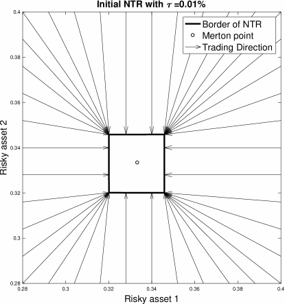
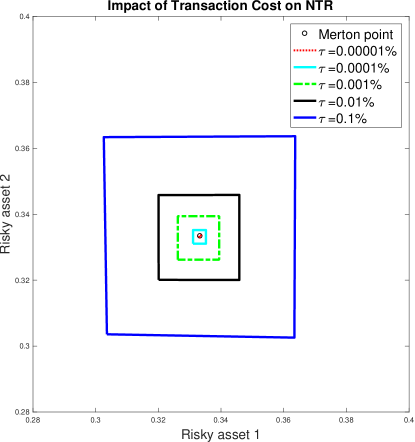
Figure 1: NTR at the initial time with various transaction costs.

The results in Figure 1 are provided by our numerical DP method, in which we choose degree-100 complete Chebyshev polynomial approximations, use $101^{2}$ tensor Chebyshev nodes as the approximation nodes to compute Chebyshev coefficients, and implement the tensor product Gauss-Hermite quadrature rule with $3^{2}$ tensor quadrature nodes. We run it on a Mac Pro with a 3.5 GHz 6-Core Intel Xeon E5 using the parallel DP method, and it takes about 1.5 wall clock hours due to the high degree polynomial approximations. To further verify that we solve the portfolio problem accurately, we employ degree-150 complete Chebyshev polynomial approximations, $151^{2}$ tensor Chebyshev nodes, and tensor product Gauss-Hermite quadrature rule with $9^{2}$ tensor quadrature nodes. We find that there is little change in the solution: e.g., the $\mathcal{L}^{1}$ difference between the degree-100 and the degree-150 solutions is $3.1\times 10^{-4}$, and the $\mathcal{L}^{\infty}$ difference is $7.1\times 10^{-4}$. A smaller degree polynomial approximation can be faster but will lead to less accurate solutions. For example, if we use degree-80 complete Chebyshev polynomial approximations and $81^{2}$ tensor Chebyshev nodes for the case with $\tau=0.01\%$, then it takes only 44 minutes, but it also provides a nontrivial change in the solutions: the $\mathcal{L}^{1}$ difference between the degree-100 and degree-89 solutions is 0.0014, and the $\mathcal{L}^{\infty}$ difference is 0.0033. Note that the kinks on the border of the NTR in the value and policy functions make it slow to improve the accuracy of the solution by increasing the degree of polynomial approximation.

Figure 2 shows the NTRs at the initial time with various time step sizes ranging from daily to monthly (the left panel) and horizons from one week to three years (the right panel), with $\tau=0.01\%$. The left panel of Figure 1 shows that the NTR with 3-year horizon expands if the time step size decreases. The right panel of Figure 2 shows that the NTR of a daily trader shrinks as the horizon increases, and the NTR with $T=0.6$ years is almost identical to the NTR with $T=3$ years. This implies that the trading strategy for infinite-horizon continuous-time problems can be approximated by the initial time solutions of a six-month horizon problem with daily time steps. This also explains why the NTRs in the right panel of Figure 1 converge to the Merton point when $\tau\rightarrow 0$.

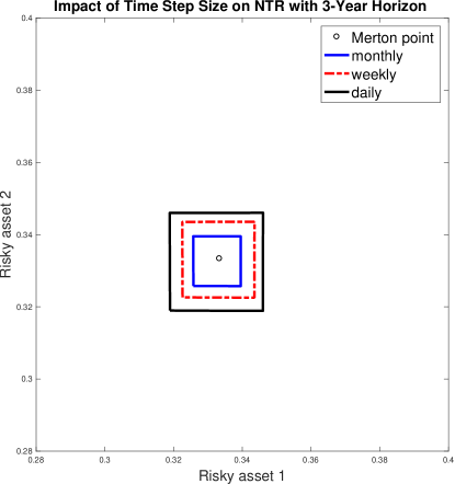
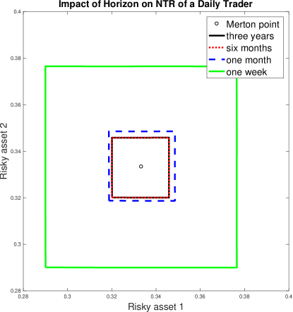
Figure 2: Initial NTR with various time step sizes and horizons.

3.2 Portfolio Problems with Consumption

In this subsection, we solve the with-consumption model (19). The assets available for trading include one risk-free asset with an interest rate $r$ and multiple risky assets with log-normal annual returns. We assume that the utility function is $U(c)=c^{1-\gamma}/(1-\gamma)$. Table 1 list values of parameters of the examples in this subsection, where $I_{4}$ represents the $4\times 4$ identity matrix.

	Example 2	Example 3	Example 4	Example 5
$k$	2	2	3	4
$\gamma$	2	3	3	4
$\tau$	1%	0.1%	0.1%	0.1%
$\beta$	$\exp(-0.1\Delta t)$	$\exp(-0.05\Delta t)$	$\exp(-0.05\Delta t)$	$\exp(-0.05\Delta t)$
$r$	0.07	0.03	0.04	0.03
$\mu^{\top}$	$(0.15,0.15)$	stochastic	$(0.07,0.07,0.07)$	$(0.06,0.066,0.072,0.078)$
$\sigma^{\top}$	$(\sqrt{0.17},\sqrt{0.17})$	$(0.2,0.2)$	$(0.2,0.2,0.2)$	$(0.2,0.23,0.26,0.29)$
$\Sigma$	$\left[\begin{array}[]{cc}1&0.4706\\ 0.4706&1\end{array}\right]$	$\left[\begin{array}[]{cc}1&0\\ 0&1\end{array}\right]$	$\left[\begin{array}[]{ccc}1&0.4&0.4\\ 0.4&1&0.16\\ 0.4&0.16&1\end{array}\right]$	$I_{4}$

Table 1: Parameters for Examples of Portfolio Problems with Consumption.

3.2.1 Example 2: a Three-Asset Problem with Consumption

For the problem with two risky assets and one risk-free asset, the parameter values are listed in Table 1, and they are either the same as or discrete-time analogs to those in Discussion 1 in Muthuraman and Kumar (2006), including $\tau=1\%$, in order to show that our numerical DP method can also solve the continuous-time infinite-horizon portfolio problem with consumption in Muthuraman and Kumar (2006). We use weekly time steps (i.e., $\Delta t=1/52$ years), and in the numerical DP method for this example, we use degree-$60$ complete Chebyshev polynomials to approximate value functions, use $61^{2}$ tensor Chebyshev nodes as the approximation nodes to compute Chebyshev coefficients, and implement the multi-dimensional product Gauss-Hermite quadrature rule with $3^{2}$ tensor quadrature nodes. For the case with $T=3$ years (i.e., $N=156$ periods), it takes only two minutes on a Mac Pro with a 3.5 GHz 6-Core Intel Xeon E5. A larger degree (e.g., degree-100) polynomial approximation (with a higher number of Chebyshev nodes) or more quadrature nodes (e.g., 5 nodes in each dimension) has little impact on the solution: e.g., the $\mathcal{L}^{1}$ difference between the degree-60 and degree-100 solutions is $4.6\times 10^{-4}$, and the $\mathcal{L}^{\infty}$ difference is 0.0013. In comparison with the no-consumption examples in Section 3.1, the with-consumption problems require a much lower degree of polynomial approximation, because the discount factor and utility of consumption in the objective of the with-consumption model (19) alleviate the impact of kinks in the value functions on the solutions.

The left panel of Figure 3 displays the NTRs at the initial time with various time step sizes ranging from daily to monthly for $T=3$ years (i.e., $N=156$ periods). The circle point located inside the NTRs is the Merton point $(0.16,0.16)$. We see that the NTR with weekly time steps is close to the NTR with daily time steps, and is also close to the solution given in Muthuraman and Kumar (2006) for the infinite-horizon portfolio optimization problems in which assets can be traded at any continuous time. Thus, we have shown that our numerical DP can solve continuous-time infinite-horizon portfolio problem with consumption. Moreover, we can use weekly time steps to approximate the continuous-time with-consumption model.

The right panel of Figure 3 shows the initial-time NTRs with various trading horizons from one month to ten years, for a fixed time step size of one week. We see that the trading horizon changes the NTR: a shorter horizon has a larger NTR. We see that the NTR of the three-year horizon is almost identical to the NTR of the ten-year horizon. Moreover, when the horizon is small, the no-shorting constraint becomes binding for some portfolios before rebalancing. For example, when the horizon has only one month, if the portfolio before re-allocation is (0,0), then the optimal trading strategy is to keep the current portfolio unchanged (i.e., the no-shorting constraint is binding). These occasionally binding constraints make it challenging for a partial differential equation solution method such as the one used in Muthuraman and Kumar (2006), but our numerical DP method can handle them. Clearly, the short-horizon NTRs are impacted by the terminal condition, i.e., the terminal value function. With our terminal value function (20) and the assumption to close all risky assets, NTRs are moving towards the origin if horizon becomes shorter, as an investor is less willing to keep risky assets so as to avoid the transaction costs incurred by selling all risky assets at the terminal time. Thus, the Merton point is no longer in the center of the NTRs for short-horizon problems and is no longer a good approximate solution, as its distance to the optimal portfolio may be more than 0.2 for the one-month-horizon problem (as shown in the right panel of Figure 3).

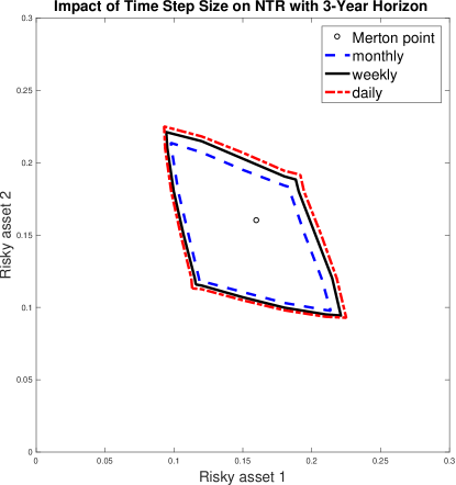
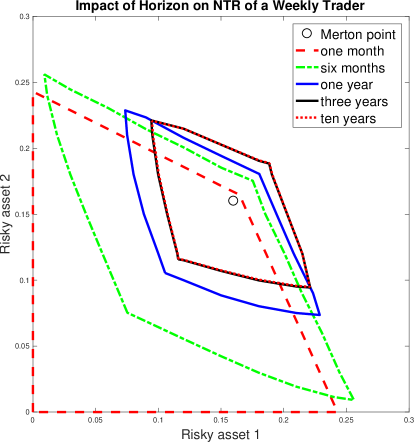
Figure 3: Impact of time step size and horizon on the initial-time NTR for 2 correlated risky assets and 1 risk-free asset with consumption.

3.2.2 Example 3: a Three-Asset Problem with Consumption and Stochastic Drift of Return

Example 2 has shown that numerical DP can solve a continuous-time infinite-horizon DP problem, which is often transformed to a Hamilton-Jacobi-Bellman partial differential equation (PDE) for being solved numerically. However, if there are stochastic and discrete parameters, then it is often challenging to solve PDEs with such jump processes. In this example, we apply numerical DP to solve a three-asset with-consumption model (19), assuming that the drifts of risky returns, $\mu_{t}=(\mu_{t,1},\mu_{t,2})^{\top}$, are stochastic. In Appendix A.2, we also solve dynamic portfolio problems with stochastic interest rates $r$ or stochastic volatility $\sigma$. We assume that $\mu_{t,1}$ and $\mu_{t,2}$ are discrete Markov chains and independent of each other. Each $\mu_{t,i}$ has two possible values: $\mu^{1}=0.06$ and $\mu^{2}=0.08$, and its transition probability matrix is

$$\left[\begin{array}[]{cc}0.75&0.25\\ 0.25&0.75\end{array}\right]$$

for each $i=1,2$, where its $(j_{1},j_{2})$ element represents the transition probability from $\mu_{t,i}=\mu^{j_{1}}$ to $\mu_{t+\Delta t,i}=\mu^{j_{2}}$, for $j_{1},j_{2}=1,2$. The other parameter values are listed in Table 1.

We use weekly time periods (i.e., $\Delta t=1/52$ years) in $T=3$ years (so the number of periods is $N=156$). The assets available for trading include one risk-free asset with an interest rate $r$ and $k=2$ uncorrelated risky assets with log-normal returns. In the numerical DP method, we choose degree-$60$ complete Chebyshev polynomials to approximate value functions, use $61^{2}$ tensor Chebyshev nodes as the approximation nodes, and implement the multi-dimensional product Gauss-Hermite quadrature rule with $3^{2}$ tensor quadrature nodes.

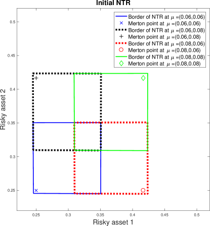
Figure 4: NTRs with a stochastic $\mu$.

Figure 4 displays the NTRs for four possible discrete states of $(\mu_{t,1},\mu_{t,2})$ at the initial time. The previous examples without stochastic parameters have only one unique NTR at each trading time, but in this example each discrete state of stochastic parameters has its own corresponding NTR. These NTRs are close to being square as the two risky assets are i.i.d.. The top-right square is the NTR for the state $(\mu_{t,1},\mu_{t,2})=(0.08,0.08)$, the bottom-left square is the NTR for the state $(\mu_{t,1},\mu_{t,2})=(0.06,0.06)$, and the top-left and the bottom-right squares are the NTRs for the states $(\mu_{t,1},\mu_{t,2})=(0.06,0.08)$ and $(\mu_{t,1},\mu_{t,2})=(0.08,0.06)$ respectively. The diamond, the mark, the plus, and the circle inside the squares are the corresponding Merton points if we assume that $(\mu_{t,1},\mu_{t,2})$ are fixed at their initial values. We see that a smaller $\mu_{t,i}$ implies a NTR and a Merton point closer to the origin of the coordinate system. This is consistent with the formula of the Merton point, (21). We see that these Merton points are no longer in the centers of the NTRs, like what the previous examples without stochastic parameters have shown (except the short-horizon problems); thus using Merton points as portfolio solution is no longer good as the difference between the optimal solution and the Merton points may be more than 0.1, as shown in Figure 4. Appendix A.2 shows more examples with stochastic interest rate or volatility, and their NTRs have similar patterns.

3.2.3 Example 4: a Four-Asset Problem with Consumption

It is often challenging for a PDE solution method to solve problems with three or more continuous state dimensions. In this example, we employ the numerical DP method to solve the with-consumption model (19) with three continuous state dimensions, in which we have one risk-free asset and three correlation risky assets available for monthly trading (i.e., $\Delta t=1/12$ years) in $T=3$ years (so there are $N=36$ periods). The parameter values are listed in Table 1. In the numerical DP method for this example, we choose degree-$60$ complete Chebyshev polynomials to approximate value functions, use $61^{3}$ tensor Chebyshev nodes as the approximation nodes to compute Chebyshev coefficients, and implement the multi-dimensional product Gauss-Hermite quadrature rule with $3^{3}$ tensor quadrature nodes. We run the parallel DP method on the Blue Waters supercomputer, and it takes nearly 2.6 wall clock hours using 640 cores. A higher degree (e.g., degree-80) polynomial approximation (with a higher number of Chebyshev nodes) or more quadrature nodes (e.g., 5 nodes in each dimension) have little change to the solution: e.g., the $\mathcal{L}^{1}$ difference between the solution from the degree-60 polynomial approximation and the solution from the degree-80 polynomial approximation is $4.7\times 10^{-4}$, and the $\mathcal{L}^{\infty}$ difference is 0.0017. Figure 5 displays the NTR at the initial time. The circle inside the NTR is the Merton point: $(0.1071,0.1786,0.1786)$. For convenience, we plot the faces of the NTR as flat, but in fact there is small curvature on the faces, and the exact NTR might have curvy faces too as Figure 3 has shown. The NTR is tilted as the risky assets are correlated.

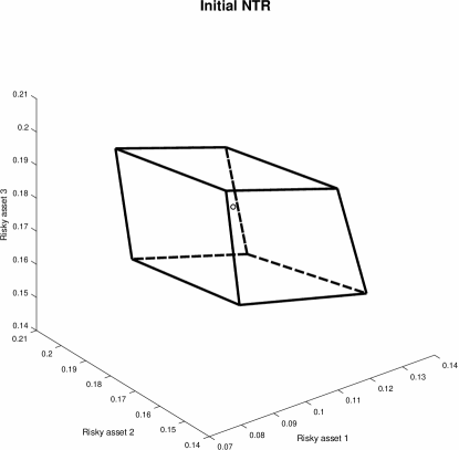
Figure 5: Initial NTR for 3 correlated risky assets and 1 risk-free asset with consumption.

3.2.4 Error Analysis for Example 4

Examples 2 and 4 have shown that computational time expands exponentially with the number of risky assets as we use tensor grids for approximation nodes and quadrature nodes. In particular, due to the existence of kinks of the value functions, we have to use high-degree polynomial approximations. In Example 4, we have used the degree-80 solution as the “true” solution to compare with lower-degree solutions. If the difference is small, we consider the solutions from the lower-degree approximations to be accurate.

However, for problems with more risky assets, we cannot use a solution from a very high degree polynomial approximation to estimate our solution’s accuracy, due to computational resource limitations. Instead, we roughly estimate our solution’s accuracy from policy approximation errors. That is, we use the solutions of optimal decisions over all approximation nodes in the state space to construct a complete Chebyshev polynomial to approximate a policy function for each decision variable, and then we compute the distances between optimal decisions over 1,000 random nodes in the state space and the values of the approximated policy functions over the same set of random nodes. These distances are called policy approximation errors. This method has been implemented in Cai et al. (2017) and Cai and Lontzek (2019).

Table 2 shows the policy approximation errors and the difference from the degree-80 solution in their $\mathcal{L}^{1}$ and $\mathcal{L}^{\infty}$ norms. We see that both the policy approximation errors and the difference from the degree-80 solution are declining over the degrees. A lower-degree approximation is computationally faster but its error is also larger. For example, using degree-8 approximation takes only 18 seconds using 6 cores, but its policy approximation error in $\mathcal{L}^{\infty}$ is 0.02, and its solution’s difference from the degree-80 solution is 0.045 in the $\mathcal{L}^{\infty}$ measurement. If we want to control the $\mathcal{L}^{\infty}$ error at around 0.005, then the degree-30 solution can suffice.

Deg.	Policy Approx. Errors		Diff. from deg-80 Sol.		Number	Time
	$\mathcal{L}^{1}$ Error	$\mathcal{L}^{\infty}$ Error	$\mathcal{L}^{1}$ meas.	$\mathcal{L}^{\infty}$ meas.	of Cores
8	0.00190	0.0203	0.0195	0.0452	6	18 seconds
20	0.00040	0.0089	0.0059	0.0152	6	12 minutes
30	0.00016	0.0062	0.0027	0.0050	256	7 minutes
40	0.00013	0.0042	0.0027	0.0046	288	37 minutes
60	0.00009	0.0027	0.0005	0.0017	640	2.6 hours

Table 2: Error Analysis and Running Times.

3.2.5 Example 5: a Five-Asset Problem with Consumption

Our last example without options solves the with-consumption model (19), where the assets available for trading include one risk-free asset and four risky assets with independent log-normal annual returns. We assume $T=3$ years and $\Delta t=1/12$ years. The parameter values are listed in Table 1.

Figure 6 displays the NTR at the initial time, and we see that the NTR is close to being a hyper-rectangle as the four risky assets are uncorrelated. The top-right rectangle (with solid lines) and the bottom-left rectangle (with dashed lines) are the cross-sections of the NTR for risky assets 1 and 2, and risky assets 3 and 4, respectively. In the figure, the circle and the mark are, respectively, the projections of the Merton point, $(0.1875,0.1701,0.155,0.1427)$, on risky assets 1 and 2, and risky assets 3 and 4.

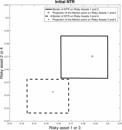
Figure 6: Initial NTR for 4 independent risky assets and 1 risk-free asset.

We choose degree-30 complete Chebyshev polynomials to approximate value functions, use $31^{4}$ tensor Chebyshev nodes to compute Chebyshev coefficients, and implement the multi-dimensional product Gauss-Hermite quadrature rule with $3^{4}$ tensor quadrature nodes. Thus, for each period, there are $31^{4}=923,521$ optimization problems in the maximization step. Moreover, the evaluation of the objective function of each optimization problem is time-consuming: the product quadrature rule means there are $3^{4}=81$ evaluations (one evaluation per quadrature node) of a degree-30 complete Chebyshev polynomial which contains $\left(\begin{array}[]{c}30+4\\ 4\end{array}\right)=46,376$ terms of Chebyshev basis polynomials. This is a computationally intensive problem. It takes about 9.8 hours to get the solution using 3,840 cores of the Blue Waters supercomputer. If we use degree-60 complete Chebyshev polynomials with $61^{4}$ tensor Chebyshev nodes, then we can improve our solution’s accuracy, but it would require too much computing resources: around

$$\frac{61^{4}\times\left(\begin{array}[]{c}60+4\\ 4\end{array}\right)}{31^{4}\times\left(\begin{array}[]{c}30+4\\ 4\end{array}\right)}\approx 205$$

times more as a rough estimate, which has exceeded our available resources in the Blue Waters supercomputer. Thus, we cannot use a solution from a very high degree polynomial approximation to estimate our solution’s accuracy, so instead we roughly estimate it using policy approximation errors, which are $2.3\times 10^{-4}$ in $\mathcal{L}^{1}$ and $0.0056$ in $\mathcal{L}^{\infty}$. These errors are close to the policy approximation errors in Example 4 with the degree-30 approximation. Thus, from Table 2, we estimate that the error of our solution in Figure 6 in comparison with the true solution would be around 0.003 in $\mathcal{L}^{1}$ and 0.005 in $\mathcal{L}^{\infty}$.

We also run an example with one risk-free asset and six uncorrelated risky assets using degree-8 complete Chebyshev polynomials to approximate value functions on the six-dimensional hypercube, and get the NTR as a six-dimensional hyper-rectangle. Its policy approximation errors are also close to those of Example 4 with the degree-8 approximation, so its error would be several percent of wealth, such that it might not be better than a solution using its Merton point for a long-horizon problem. However, for such a high-dimensional problem, our numerical DP method can provide a NTR which might still be better than a Merton point, when the problem has a short horizon or stochastic parameters, in which the distance between the Merton point and the true NTR could be relatively large, as shown in the right panel of Figure 3 or Figure 4.

4 Pricing Formula for Options

We first give the pricing formula for a put option. Let the expiration time of the put option be $T$, and let its strike price be $K$. Then the payoff of the put option at the expiration time $T$ is $\max(K-S_{T},0)$, where $S_{T}$ is the price of the underlying risky asset at time $T$. We assume that the price $S_{t}$ of the underlying asset follows a geometric Brownian motion process with constant drift $\mu$ and volatility $\sigma$, and the risk-free interest rate is $r$. Black and Scholes (1973) give an explicit risk-neutral pricing formula for the European-type put option at time $t<T$. However, some other kinds of options cannot have an explicit formula. For example, an American-type put option has to use some numerical methods for its pricing. One general numerical method for pricing is the binomial lattice method (see e.g., Luenberger 1997), which can be used for pricing both American-type and European-type options.

In the binomial lattice model, we set $h$ as a sub-period length and $n$ as the number of sub-periods such that $nh=\Delta t$, where $\Delta t$ is the length of one period in the multi-period portfolio optimization model (i.e., investors can rebalance their portfolio every time $\Delta t$). If the price is known as $S$ at the beginning of a sub-period, the price at the beginning of the next sub-period is $Su$ or $Sd$, with $u>1$ and $0<d<1$. The probability of the upward movement is $p$, and the probability of the downward movement is $1-p$. To match the log-normal assumption of the risky asset return, we follow the binomial lattice method to assume that

$$\left\{\begin{array}[]{l}p=\frac{1}{2}+\frac{\mu-\sigma^{2}/2}{2\sigma}\sqrt{h},\\ u=\exp(\sigma\sqrt{h}),\\ d=\exp(-\sigma\sqrt{h}),\end{array}\right.$$ (22)

such that the expected growth rate of $\log(S)$ in the binomial model converges to $(\mu-\sigma^{2}/2)$, and the variance of the rate converges to $\sigma^{2}$, as $h$ goes to zero. The risk-free return of one sub-period is $\exp(rh)$, and the risk-free return of one period is $R_{f}=(\exp(rh))^{n}=\exp(r\Delta t)$. Thus, the value of one sub-period put option over the underlying risky asset governed by the binomial lattice is given as

$$P=\exp(-rh)(qP_{u}+(1-q)P_{d}),$$

where $P_{u}$ and $P_{d}$ are the values at the upward branch and the downward branch at the end of this sub-period respectively, and $q$ is the risk-neutral probability with

$$q=(\exp(rh)-d)/(u-d).$$

Since the payoff of the put option at the expiration time $T$ is $P_{T}=\max(K-S_{T},0)$, we can compute the price of the put option at any binomial node by applying the above backward iterative relation. From the above binomial model, we know that the risky asset return of one period, $R$, has the following probability distribution:

$$\Pr(R=u^{j}d^{n-j})=\frac{n!}{j!(n-j)!}p^{j}(1-p)^{n-j}$$ (23)

for $j=0,1,\ldots,n,$ where $p,u$, and $d$ are defined in (22).

We also use the same binomial lattice method to price a call option. The computational process is the same as for the put option, except we need to set the payoff of the call option at the expiration time $T$ as $P_{T}=\max(S_{T}-K,0)$ for a pre-specified strike price $K$. The binomial lattice method will also be used to price a butterfly option, a combination of a call option and a put option with the same strike price. That is, the payoff of the butterfly option at the expiration time is $P_{T}=\left|S_{T}-K\right|$.

5 DP Models with Options

We solve dynamic portfolio problems with a portfolio including a risk-less asset, an option, and its underlying risky asset. We assume that the option has an expiration time $T$ and a strike price $K$, and it is available for trading at times $t=t_{0},t_{1},t_{2},\ldots,t_{N}$ with $t_{j}=j\Delta t$ for $j=0,1,...,N$ and $\Delta t=T/N$, with a price process $P_{t}$, while its underlying risky asset’s price process is $S_{t}$. Since the option price $P_{t}$ is dependent on $S_{t}$ and $K$, we denote it as $P_{t}(S_{t},K)$ explicitly. Right before reallocation time $t$, assume that $W_{t}$ is the wealth, $X_{t}$ is the amount of money invested in the risky asset, and $Y_{t}$ is the amount of money invested in the option. Since the price of the option is dependent on the risky asset price, we should add $S_{t}$ as a state variable. That is, there are four state variables: $W_{t},X_{t},Y_{t},S_{t}$. Denote $A_{t}=S_{t}/K$. Since the payoff of a put option is $P_{T}=\max(K-S_{T},0)=K\cdot\max(1-A_{T},0)$, we have $P_{t}(S_{t},K)=KP_{t}(A_{t},1)$ by replication. For simplicity, we denote $P_{t}(A_{t})=P_{t}(A_{t},1)$, so

$$\frac{P_{t+\Delta t}(S_{t+\Delta t},K)}{P_{t}(S_{t},K)}=\frac{P_{t+\Delta t}(A_{t+\Delta t})}{P_{t}(A_{t})}.$$

Similarly, for a call option or a butterfly option, the separation of $K$ and $A_{t}$ still hold. Thus, we can use $A_{t}$ as the state variable instead of $S_{t}$.

Assume that $\Delta X_{t}$ is the amount of dollars for buying or selling the risky asset at time $t$, and $\Delta Y_{t}$ is the amount of dollars for buying or selling the option. $\Delta X_{t}>0$ or $\Delta Y_{t}>0$ means buying the risky asset or the option, while $\Delta X_{t}<0$ and $\Delta Y_{t}<0$ means selling the risky asset and the option. We assume that there are proportional transaction costs in buying or selling the risky asset and the option, with the proportions $\tau_{1}$ and $\tau_{2}$ respectively. Thus, the transition laws of the four state variables in one period with time length $\Delta t$ are

$$A_{t+\Delta t} = A_{t}R,$$ (24)

$$Y_{t+\Delta t} = (Y_{t}+\Delta Y_{t})\frac{P_{t+\Delta t}(A_{t+\Delta t})}{P_{t}(A_{t})},$$ (25)

$$X_{t+\Delta t} = R(X_{t}+\Delta X_{t}),$$ (26)

$$W_{t+\Delta t} = R_{f}(W_{t}-X_{t}-Y_{t}-Z_{t})+X_{t+\Delta t}+Y_{t+\Delta t},$$ (27)

where $R$ is the random return of the risky asset in one period with length $\Delta t$, $R_{f}=\exp(r\Delta t)$ is the one-period risk-free return with $r$ the interest rate, and

$$Z_{t}=\Delta X_{t}+\Delta Y_{t}+\tau_{1}\left|\Delta X_{t}\right|+\tau_{2}\left|\Delta Y_{t}\right|.$$ (28)

We also assume that there are constraints in shorting risky assets/options or borrowing cash. For simplicity, we assume that neither shorting nor borrowing is allowed. That is, we have the following constraints:

$$X_{t}+\Delta X_{t} \geq 0,$$ (29)

$$Y_{t}+\Delta Y_{t} \geq 0,$$ (30)

$$X_{t}+Y_{t}+Z_{t} \leq W_{t}.$$ (31)

Thus, the DP model is

$$V_{t}(W_{t},X_{t},Y_{t},A_{t})=\max_{\Delta X_{t},\Delta Y_{t}}\text{ }\mathbb{E}_{t}\left\{V_{t+\Delta t}(W_{t+\Delta t},X_{t+\Delta t},Y_{t+\Delta t},A_{t+\Delta t})\right\},$$ (32)

subject to the constraints (24)-(31), for $t=t_{0},t_{1},t_{2},\ldots,t_{N-1}$. Here, $\mathbb{E}_{t}$ is the expectation operator conditional on the information at time $t$, and the terminal value function is $V_{T}(W,X,Y,S)=U(W)$ for some given utility function $U$.

5.1 Problems without Consumption

In order to use a smooth optimization solver for solving the DP model, we want to cancel out the absolute operator in the constraint (28). This can be done by letting $\Delta X_{t}=W_{t}(\delta_{tx}^{+}-\delta_{tx}^{-})$ and $\Delta Y_{t}=W_{t}(\delta_{ty}^{+}-\delta_{ty}^{-})$, with $\delta_{tx}^{+},\delta_{ty}^{-}\geq 0$ such that $\left|\Delta X_{t}\right|$ and $\left|\Delta Y_{t}\right|$ can be substituted by $W_{t}(\delta_{tx}^{+}+\delta_{tx}^{-})$ and $W_{t}(\delta_{ty}^{+}+\delta_{ty}^{-})$ respectively in the optimization problems.

If the utility function is CRRA with relative risk aversion coefficient $\gamma>0$, then we let $x_{t}=X_{t}/W_{t}$ and $y_{t}=Y_{t}/W_{t}$. By using $W_{t},x_{t},y_{t}$, and $A_{t}$ as state variables, we can separate $W_{t}$ and $(x_{t},y_{t},A_{t})$ in the value function $V_{t}(W_{t},x_{t},y_{t},A_{t})$. When $U(W)=W^{1-\gamma}/(1-\gamma)$ with $\gamma>0$ and $\gamma\neq 1$, we have

$$V_{t}(W_{t},x_{t},y_{t},A_{t})=W_{t}^{1-\gamma}\cdot g_{t}(x_{t},y_{t},A_{t}),$$ (33)

where

$$g_{t}(x_{t},y_{t},A_{t})=\max_{\delta_{tx}^{+},\delta_{tx}^{-},\delta_{ty}^{+},\delta_{ty}^{-}\geq 0}\text{ }\mathbb{E}_{t}\left\{\Pi_{t+\Delta t}^{1-\gamma}\cdot g_{t+\Delta t}(x_{t+\Delta t},y_{t+\Delta t},A_{t+\Delta t})\right\},$$ (34)

subject to

$$A_{t+\Delta t} = A_{t}R,$$ (35)

$$\xi_{t+\Delta t} = R(x_{t}+\delta_{tx}^{+}-\delta_{tx}^{-}),$$ (36)

$$\eta_{t+\Delta t} = (y_{t}+\delta_{ty}^{+}-\delta_{ty}^{-})\frac{P_{t+\Delta t}(A_{t+\Delta t})}{P_{t}(A_{t})},$$ (37)

$$z_{t} = \delta_{tx}^{+}-\delta_{tx}^{-}+\delta_{ty}^{+}-\delta_{ty}^{-}+\tau_{1}(\delta_{tx}^{+}+\delta_{tx}^{-})+\tau_{2}(\delta_{ty}^{+}+\delta_{ty}^{-}),$$ (38)

$$\Pi_{t+\Delta t} = R_{f}(1-x_{t}-y_{t}-z_{t})+\xi_{t+\Delta t}+\eta_{t+\Delta t},$$ (39)

$$x_{t+\Delta t} = \xi_{t+\Delta t}/\Pi_{t+\Delta t},$$ (40)

$$y_{t+\Delta t} = \eta_{t+\Delta t}/\Pi_{t+\Delta t},$$ (41)

and the following no-shorting and no-borrowing constraints

$$x_{t}+\delta_{tx}^{+}-\delta_{tx}^{-} \geq 0,$$ (42)

$$y_{t}+\delta_{ty}^{+}-\delta_{ty}^{-} \geq 0,$$ (43)

$$x_{t}+y_{t}+z_{t} \leq 1.$$ (44)

The terminal function is $g_{T}(x,y,A)=1/(1-\gamma)$. Similarly, when $U(W)=\log(W)$, we can also separate $W_{t}$ and $(x_{t},y_{t},A_{t})$ in the value function $V_{t}(W_{t},x_{t},y_{t},A_{t})$. The approximation domain of $(x_{t},y_{t})$ can be set as $[0,1]^{2}$ as we do not allow shorting or borrowing.

Similarly to what we computed in the portfolio problems without options, we will also compute a no-trade region, $\Omega_{t}$, for the problems with options, in which $\Omega_{t}$ is defined as

$$\Omega_{t}=\{(x_{t},y_{t}):\ (\delta_{tx}^{+})^{\ast}=(\delta_{tx}^{-})^{\ast}=(\delta_{ty}^{+})^{\ast}=(\delta_{ty}^{-})^{\ast}=0\},$$

where $(\delta_{tx}^{+})^{\ast},(\delta_{ty}^{+})^{\ast}\geq 0$ are optimal fractions of wealth for buying the risky asset and the option, and $(\delta_{tx}^{-})^{\ast},(\delta_{ty}^{-})^{\ast}\geq 0$ are optimal fractions of wealth for selling the risky asset and the option, for a given $(x_{t},y_{t},A_{t})$. From the separability of $W_{t}$ and $(x_{t},y_{t},A_{t})$, we see that the optimal portfolio rules are independent of wealth $W_{t}$. Thus the no-trade regions $\Omega_{t}$ are also independent of $W_{t}$, for CRRA utility functions.

5.2 Long Horizon Problems with Consumption and Epstein–Zin Preferences

In some problems, assets are used to finance consumption during the period $t$. Like what we discussed in Section 2.1, if the utility function for consumption is $U(C)=C^{1-\gamma}/(1-\gamma)$ and the terminal value function is $V_{T}(W,x,y,A)=W^{1-\gamma}\cdot g_{T}(x,y,A)$ for some given $g_{T}(x,y,A)$, then the Bellman equation (34) changes to

$$g_{t}(x_{t},y_{t},A_{t})=\max_{c_{t},\delta_{tx}^{+},\delta_{tx}^{-},\delta_{ty}^{+},\delta_{ty}^{-}\geq 0}\text{ }U(c_{t})\Delta t+\beta\mathbb{E}_{t}\left\{\Pi_{t+\Delta t}^{1-\gamma}\cdot g_{t+\Delta t}(x_{t+\Delta t},y_{t+\Delta t},A_{t+\Delta t})\right\},$$ (45)

subject to the constraints (35)-(38), (40)-(43), and

$$\Pi_{t+\Delta t}=R_{f}(1-x_{t}-y_{t}-z_{t}-c_{t}\Delta t)+\xi_{t+\Delta t}+\eta_{t+\Delta t},$$

$$x_{t}+y_{t}+z_{t}+c_{t}\Delta t\leq 1,$$

where $\beta=\exp(-\rho\Delta t)$ is the one-period discount factor. The terminal value function is

$$g_{T}(x_{T},y_{T},A_{T})=\frac{U(r(1-\tau_{1}x_{T}))\Delta t}{1-\beta}=\frac{(r(1-\tau_{1}x_{T}))^{1-\gamma}\Delta t}{(1-\beta)(1-\gamma)}$$ (46)

by assuming that the agent sells all of the underlying risky asset (incurring proportional transaction cost $\tau_{1}$) and exercises all the options (without transaction costs) at the terminal time, and then consumes only the interest of the terminal wealth forever.

In the model (45), $\gamma$ is the risk aversion parameter, but it is also the inverse of the intertemporal elasticity of substitution (IES). Epstein and Zin (1989) introduce a recursive utility function to separate risk aversion and IES. If we use Epstein–Zin preferences and $U(c)=c^{1-\gamma}/(1-\gamma)$ with $\gamma$ the inverse of IES, then the Bellman equation (45) becomes

$$g_{t}(x_{t},y_{t},A_{t})=\max_{c_{t},\delta_{tx}^{+},\delta_{tx}^{-},\delta_{ty}^{+},\delta_{ty}^{-}\geq 0}\text{ }U(c_{t})\Delta t+\beta\left[\mathbb{E}_{t}\left\{\left(\Pi_{t+\Delta t}^{1-\gamma}\cdot g_{t+\Delta t}(x_{t+\Delta t},y_{t+\Delta t},A_{t+\Delta t})\right)^{\frac{1-\psi}{1-\gamma}}\right\}\right]^{\frac{1-\gamma}{1-\psi}},$$ (47)

where $\psi$ is the risk aversion parameter. See Cai et al. (2017) and Cai and Lontzek (2019) for more discussion on Epstein–Zin preferences and its use in dynamic stochastic optimization problems (e.g., the Bellman equation (47) formula holds only when $0<\gamma<1$; when $\gamma>1$, it needs some adjustment).

In reality, the time to maturity of options is typically not more than one year. Thus, if we want to solve a multi-year portfolio optimization problem with options (where each period is equal to or less than 1 year), we need to liquidate the option at its expiration time and buy some newly issued options at some intermediate stages. For simplicity, we assume that all options have the same maturity $T$ while the whole trading horizon is $mT$ (that is, we have $m$ rounds of option issuing), and at the new option issuing times $t\in{\cal I}\equiv\{0,T,2T,\ldots,(m-1)T\}$, only the at-the-money options are available (i.e., the strike price $K$ for an option issued at time $t\in{\cal I}$ is $S_{t}$, so the strike prices will be different for these different at-the-money options issued at different times). Thus, when $t\not\in{\cal I}$ or $t=0$, the DP model is the same as (32).

When $t\in{\cal I}$ and $t>0$, we use $t^{+}$ to denote the time right after liquidating the expired options and before rebalancing with newly issued options. We assume that there is no transaction cost for liquidating the expired options. Thus, we have $Y_{t^{+}}=0$ and $W_{t^{+}}=W_{t}$ (while the cash amount increases from $W_{t}-X_{t}-Y_{t}$ to $W_{t}-X_{t}$). Moreover, since we assume that only an at-the-money option is available for trading no matter what the risky asset price is at time $t\in{\cal I}$, we have $A_{t^{+}}=1$. That is, we have

$$V_{t}(W_{t},X_{t},Y_{t},A_{t})=V_{t^{+}}(W_{t^{+}},X_{t^{+}},0,1)=V_{t^{+}}(W_{t},X_{t},0,1)=W_{t}^{1-\gamma}\cdot g_{t}(x_{t},0,1),$$

for $t\in{\cal I}$ and $t>0$, because we assume that there is no transaction cost for liquidating the expired options.

6 Examples with Options

In all examples in this section, we assume that the available assets for trading are one risk-free asset, one risky asset, and one option underlying the risky asset. The risk-free asset has an annual interest rate, $r=0.01$. The risky asset has a return $R$ drawn from the binomial distribution (23) with $\mu=0.07$, $\sigma=0.2$, and a proportional transaction cost ratio $\tau_{1}$. The option has an expiration time $T$ and a strike price $K$ specified at its issue time and a proportional transaction cost ratio $\tau_{2}$. The terminal value function is $U(W)=W^{1-\gamma}/(1-\gamma)$ with the default $\gamma=3$ for the problems without consumption. The default length of one period is $\Delta t=1/52$ years, i.e., one week. We apply the binomial lattice model (22) with the default length of one sub-period $h=1/520$ (so the default number of sub-periods is $n=\Delta t/h=10$).

In the following examples, our approximation method in numerical DP uses degree-100 complete Chebyshev polynomials with $101^{2}$ Chebyshev nodes in two continuous states: $(x_{t},y_{t})$, where $x_{t}$ and $y_{t}$ are the fractions of wealth invested in the risky asset and the option at the time right before the reallocation time $t$ respectively. Similarly to our examples without options, we use the square $[0,1]^{2}$ as the approximation domain for $(x_{t},y_{t})$, and we choose a degree-100 polynomial approximation as a higher degree approximation (with a higher number of approximation nodes) has little change in the solution. Here we do not need the Gauss-Hermite quadrature rule as we have already discretized the price of the risky asset and keep it as a discrete state variable.

6.1 Portfolio with a Put Option

Our first example with options chooses the at-the-money put option (i.e., the strike price $K=S_{0}$ or equivalently $A_{0}=1$) with the expiration time $T=0.5$ years. The trading horizon is also $T$, so it has 26 re-allocation times with the weekly time steps, and 261 sub-periods over the whole horizon (so the largest number of values of the discrete state $A_{t}$ is 261, which happens at the terminal time). Figure 7 shows the NTRs and the optimal transaction paths in arrows at the initial time for $\tau_{1}=\tau_{2}=0.001$ (the left panel) and $\tau_{1}=0.001$ and $\tau_{2}=0.002$ (the right panel), where the horizontal and vertical axes represent the fraction of wealth invested in the underlying risky asset and the option respectively (the axes of all other figures in this section have the same meaning). The circle on the horizontal axis is the Merton point, $(0.5,0)$, if we assume that the underlying risky asset can be traded at any time without transaction costs so that the option can be replicated completely by the risk-free asset and the underlying risky asset (then there is zero fraction of wealth invested in the option at the Merton point).

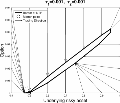
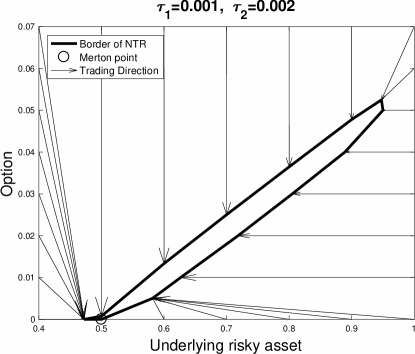
Figure 7: Initial NTRs for 1 underlying risky asset, 1 put option, and 1 risk-free asset.

Since the payoff of the put option at the expiration time is $\max(K-S_{T},0)$, we know that the put option is negatively and highly correlated with the underlying risky asset. The high correlation of the underlying risky asset and the option implies that the objective function of the optimization problem is flat so the NTR should be a strip that is close to a line, and the strip should be tilted toward one axis. The negative correlation implies that the strip should be tilted with a positive slope. All these properties can be observed in Figure 7, while the right panel’s strip is slightly wider than the left panel’s, due to the larger transaction cost of the option.

The arrows in Figure 7 show the paths from the initial allocations on the border of the axis box to the optimal allocations. In the left panel of Figure 7 (with $\tau_{1}=\tau_{2}=0.001$), we see that if the initial allocation of wealth is 47% or less, then the optimal decision is to sell all put options and buy some risky assets until the point (0.47,0). This happens because the put options are for hedging risks, so if the fraction of risky assets is small, the whole portfolio’s risk is small and it becomes inefficient to hold the put options. Moreover, if the initial allocation of wealth is 80% or more in the underlying risky asset and 0% in the put option, then the optimal decision is to sell some of the risky asset until its fraction becomes 75% and to buy some put options until its fraction becomes 2.4%, in order to hedge risks. Otherwise, holding too many risky assets may incur too large a loss of wealth if the return of the risky asset turns out to be small. Furthermore, if the initial allocation of wealth is between 60% and 75% in the underlying risky asset and 0% in the put option, then to hedge risks the optimal decision is to keep the same amount of the risky asset but to buy put options until the lower envelope of the NTR is reached. However, in the right panel of Figure 7 (with $\tau_{1}=0.001$ and $\tau_{2}=0.002$), if the initial allocation of wealth is 60% or more in the underlying risky asset and 0% in the put option, then the optimal decision is to sell some of the risky asset until its fraction becomes 58% and to buy some put options until its fraction becomes 0.5%. That is, the higher transaction cost for options makes an investor less willing to buy options, and hold less of the risky asset as the need for risk hedging from put options is also less.

For each initial risky asset allocation fraction from 0 to 1, while the initial option allocation fraction is 0, we can compute the optimal trading strategy for the dynamic portfolio problem, and then we can compute its certainty equivalent, which is the certain amount giving the same utility as the expected utility of uncertain future wealth. Figure 8 shows the functions of certainty equivalents over the initial risky asset allocation fraction for five cases. Its horizontal axis is the NTR of the underlying risky asset with $\tau_{1}=0.001$ when there is no option available for trading. The solid line represents the case where there is no option available for trading, and the other four lines (circled, dotted, dash-dotted, dashed) represent the cases with different transaction cost ratios, $\tau_{2}$, for the available option. The figure shows that the put option contributes to the certainty equivalents. If the allocation fraction in the underlying risky asset is higher, then the difference is higher, as an investor requires more put options to hedge risks. Moreover, if $\tau_{2}$ is smaller, then the corresponding certainty equivalent with the put option is higher, as the option with smaller transaction costs becomes more attractive to investors.

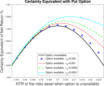
Figure 8: Certainty equivalents for put options with various transaction costs.

From Figure 8, we see that when the initial risky asset allocation fraction is 52.8% of the wealth (the upper bound of the NTR without options), the difference of the certainty equivalent between the case with the put option with $\tau_{2}=0.001$ and the case without options is less than 0.001%. That is, the social value of one put option is less than 0.00001 dollars per dollar of investment if initially 52.8% of total wealth is invested in its underlying risky asset and the remained amount of the wealth is invested in the risk-free asset.

6.2 Portfolio with a Call Option

Our second example with options uses an at-the-money call option (i.e., the strike price $K=S_{0}$ or equivalently $A_{0}=1$) in the portfolio. Other parameter values are the same as the previous example. The left panel of Figure 9 shows the NTR and the optimal transaction paths in arrows. We see that the NTR is a narrow strip with a negative slope. This is caused by the positive high correlation between the call option and its underlying risky asset, as the payoff of the call at the expiration time is $\max(S_{T}-K,0)$. Moreover, if the initial allocation fraction in the risky asset is bigger than 0.53, then the optimal decision is to sell all options and to sell some of the risky asset until the boundary of the NTR (i.e., the point $(0.53,0)$) is reached. Furthermore, if the initial portfolio holds the risky asset with 40% or less of wealth and zero options, then the optimal decision is to buy the call option until the lower envelope of the NTR is reached.

The right panel of Figure 9 shows the functions of the certainty equivalents of the expected utility of future wealth over the initial allocation fraction of wealth in the underlying risky asset for five cases. Similarly to the cases with the put option, Figure 9 shows that the call option contributes to the certainty equivalents, and that the call option is more useful when the initial allocation in the risky asset is smaller. Moreover, if the transaction cost ratio for the call option is smaller, then the corresponding certainty equivalent with the call option is higher, which is consistent with the intuition that investors like to invest more in assets with lower transaction costs.

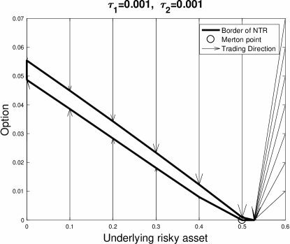
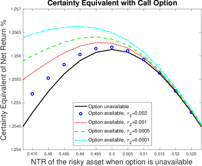
Figure 9: Initial NTR and certainty equivalents for call options.

6.3 Portfolio with a Butterfly Option

Our third example with options uses an at-the-money butterfly option in the portfolio. Other parameter values are the same as the previous example. The left panel of Figure 10 shows the NTR and the optimal transaction paths in arrows. We see that the NTR is not a narrow strip like what the previous two examples showed. Its shape is reasonable because the butterfly option is equivalent to a combination of an at-the-money put option and an at-the-money call option, and its payoff at the expiration time is $\left|S_{T}-K\right|$. Moreover, the optimal decision is to not buy any butterfly option in the case with $\tau_{1}=\tau_{2}=0.001$. This is also reflected in the right panel of Figure 10, which shows that the butterfly option has almost no contribution to the certainty equivalents. This happens because the price of the butterfly is the sum of the prices of the call and the put, so it becomes less profitable for investment.

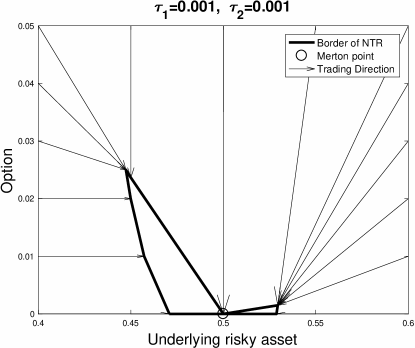
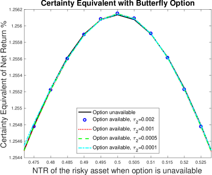
Figure 10: Initial NTR and certainty equivalents for butterfly options.

6.4 Long-Horizon Examples with Consumption and Epstein–Zin Preferences

We solve the long-horizon model in Section 5.2, which also includes consumption financed by assets, and we use Epstein–Zin preferences. The trading horizon is three years and $\tau_{1}=\tau_{2}=0.001$. The expiration time of each newly-issued at-the-money put option is $T=0.5$ years. The portfolio is rebalanced every week (i.e., $\Delta t=1/52$ years) so it has 156 periods. Every six months there is a newly-issued at-the-money put option available for trading. That is, at times $t=0.5$, 1, 1.5, 2, 2.5 years, we have a new at-the-money put option available for buying, while its older put option has to be exercised, so the largest number of discrete values of $A_{t}$ is 261, which happens at the maturity times of the option. Following Cai et al. (2017) and Cai and Lontzek (2019), we choose the utility discount rate to be $\rho=0.015$ (i.e., the one-period utility discount factor is $\beta=\exp(-\rho\Delta t)$), $\gamma=2$ or 2/3 (i.e., IES is 0.5 or 1.5), and the degree of risk aversion (RA) $\psi=2$ or 5. Our numerical DP method employs degree-100 complete Chebyshev polynomials to approximate values functions for every discrete state. We use 1,600 cores of the Blue Waters supercomputer and it takes about 1.3 hours for each case of IES and RA.

Figure 11 shows the NTRs for the four cases of IES and RA. We see that a more risk averse investor chooses to hold smaller amounts of risky assets and options, just like what their Merton points show, so RA does have significant impact on the NTR. Meanwhile, IES has little impact on the NTR: when RA=5, the difference between the NTRs when IES=0.5 and IES=1.5 is almost invisible in Figure 11.

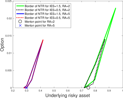
Figure 11: NTRs for problems with consumption and Epstein-Zin preferences.

However, IES impacts the optimal consumption rate: when RA=5, the optimal consumption rate is around 0.012 when IES=0.5, increasing to around 0.018 when IES=1.5, while the impact of RA on the optimal consumption is small. That is, a larger IES implies a larger consumption at the initial time, when the interest rate $r$ is lower than the utility discount rate $\rho$. This can be explained intuitively by a simple dynamic programming problem: an investor maximizes $\sum_{j=0}^{\infty}\beta^{j}U(c_{t_{j}})\Delta t$ subject to $W_{t+\Delta t}=R_{f}W_{t}-c_{t}\Delta t$ for any $t=t_{0},t_{1},t_{2},...$, that is, the only available asset for investment is the risk-free asset. It has the Euler equation: $U^{\prime}(c_{t})=\beta R_{f}U^{\prime}(c_{t+\Delta t})$. If $U(c)=c^{1-\gamma}/(1-\gamma)$, so its annual consumption growth rate at the period $(t,t+\Delta t)$ is $g_{t}\equiv\ln(c_{t+\Delta t}/c_{t})/\Delta t=(r-\rho)/\gamma$ , consistent with the famous Ramsey growth theory. That is, if $r<\rho$, then consumption growth is negative, and a smaller $\gamma$ (i.e., a larger IES) implies a larger magnitude of negative growth of consumption, so then initial consumption is larger. With Epstein-Zin preferences and risky assets including options, if RA is very large, then almost all money would be invested in the risk-free asset; this implies that a larger IES leads to a larger consumption at the initial time. We also verify this intuition numerically by solving the same long-horizon examples except with $r$ increased to $0.02$. In the cases with $r=0.02>\rho=0.015$, we find that a larger IES leads to smaller consumption at the initial time numerically, as a higher interest rate implies that future wealth could be much larger if initial consumption is smaller. This finding is also similar to what Cai et al. (2017) and Cai and Lontzek (2019) find for the impact of IES and RA on social cost of carbon.

We also run examples with ten years as the trading horizon while other parameters (including $r=0.01$) are unchanged. We find that the NTRs of the ten-year-horizon problems are almost identical to the NTRs of the three-year-horizon problems at the initial time.

7 Conclusion

This paper has shown that numerical DP can solve multi-stage portfolio optimization problems with multiple assets and transaction costs in an efficient and accurate manner. We illustrate trading strategies by describing the no-trade regions for various choices of asset returns and transaction costs. The numerical DP algorithms may be computationally intensive for large portfolio optimization problems, but modern hardware and parallel DP algorithms make it possible to solve such big problems. This paper has also shown that when there are transaction costs and constraints in shorting or borrowing, there exists a thin no-trade region for the portfolio of an option and its underlying risky asset. Future research could incorporate sparse grid methods to solve even larger dynamic portfolio problems.

Online Appendices

A.1 Numerical DP Algorithms

If the state and control variables in a DP problem are continuous, then the value function must be approximated in some computationally tractable manner. It is common to approximate value functions with a finitely parameterized collection of functions; that is, we use some functional form $\hat{V}(\mathbf{x};{\bf b})$, where ${\bf b}$ is a vector of parameters, and approximate a value function, $V(\mathbf{x})$, with $\hat{V}(\mathbf{x};{\bf b})$ for some parameter value ${\bf b}$. For example, $\hat{V}$ could be a linear combination of polynomials where ${\bf b}$ would be the weights on polynomials. After the functional form is fixed, we focus on finding the vector of parameters, ${\bf b}$, such that $\hat{V}(\mathbf{x};{\bf b})$ approximately satisfies the Bellman equation.

Numerical solutions to a DP problem are based on the Bellman equation:

$$V_{t}(\mathbf{x},\mathbf{\mathbf{\theta}})=\max_{\mathbf{a}\in{\cal D}(\mathbf{x},\mathbf{\mathbf{\theta}},t)}\text{ \ }U_{t}(\mathbf{x},\mathbf{a})+\beta\mathbb{E}_{t}\left\{V_{t+\Delta t}(\mathbf{x}^{+},\mathbf{\mathbf{\theta}}^{+})\right\},$$ (A.1)

$$\text{{\rm\ \ \ \ \ \ \ \ \ \ \ \ \ \ \ \ s.t. \ \ }}\mathbf{x}^{+}=\mathbf{\mathcal{G}}_{t}(\mathbf{x},\mathbf{\mathbf{\theta}},\mathbf{a},\mathbf{\omega}),$$

$$\text{{\rm\ \ \ \ \ \ \ \ \ \ \ \ \ \ \ \ \ \ \ \ \ \ \ }}\mathbf{\mathbf{\theta}}^{+}=\mathbf{\mathcal{H}}_{t}(\mathbf{\mathbf{\theta}},\mathbf{\epsilon}),$$

where $\mathbf{x}$ is the vector of continuous states in $\mathbb{R}^{k}$ (in our portfolio examples, $k$ is the number of risky assets including options), $\mathbf{\mathbf{\theta}}$ is the vector of discrete states in a finite set $\Theta$, $V_{t}(\mathbf{x},\mathbf{\mathbf{\theta}})$ is called the value function at time $t\leq T$ (the terminal value function $V_{T}(\mathbf{x},\mathbf{\mathbf{\theta}})$ is given), $\mathbf{a}$ is the action variable vector in its feasible set ${\cal D}(\mathbf{x},\mathbf{\mathbf{\theta}},t)$, $\mathbf{x}^{+}$ is the next-stage continuous state vector with its transition function $\mathbf{\mathcal{G}}_{t}$, $\mathbf{\mathbf{\theta}}^{+}$ is the next-stage discrete state vector with its transition function $\mathbf{\mathcal{H}}_{t}$, $\mathbf{\omega}$ and $\mathbf{\epsilon}$ are two vectors of random variables, and $U_{t}(\mathbf{x},\mathbf{a})$ is the utility function, $\beta$ is the discount factor, and $\mathbb{E}_{t}\{\cdot\}$ is the expectation operator conditional on information at time $t$.

The following is the algorithm of the numerical DP with value function iteration for finite horizon problems.

Algorithm

1. Numerical Dynamic Programming with Value Function Iteration for Finite Horizon Problems

Initialization.

Choose the approximation nodes, $\mathbb{X}=\{\mathbf{x}_{i}:$ $1\leq i\leq M\}\subset\mathbb{R}^{k}$, for every $t<T$, and choose a functional form for $\hat{V}(\mathbf{x},\mathbf{\mathbf{\theta}};{\bf b})$. Let $\hat{V}(\mathbf{x},\mathbf{\mathbf{\theta}};{\bf b}_{T})\equiv V_{T}(\mathbf{x},\mathbf{\mathbf{\theta}})$. Then for $t=t_{N-1},t_{N-2},\ldots,t_{0}$, iterate through steps 1 and 2.

Step

1. Maximization Step. Compute

$$v_{i,j}=\max_{\mathbf{a}\in{\cal D}(\mathbf{x}_{i},\mathbf{\mathbf{\theta}}_{j},t)}\ U_{t}(\mathbf{x}_{i},\mathbf{a})+\beta\mathbb{E}\left\{\hat{V}(\mathbf{x}^{+},\mathbf{\mathbf{\theta}}^{+};{\bf b}_{t+\Delta t})\right\}$$

$$\text{{\rm\ \ \ \ \ \ \ \ \ \ \ \ \ s.t. \ \ \ }}\mathbf{x}^{+}=\mathbf{\mathcal{G}}_{t}(\mathbf{x}_{i},\mathbf{\mathbf{\theta}}_{j},\mathbf{a},\mathbf{\omega}),$$

$$\text{{\rm\ \ \ \ \ \ \ \ \ \ \ \ \ \ \ \ \ \ \ \ \ \ }}\mathbf{\mathbf{\theta}}^{+}=\mathbf{\mathcal{H}}_{t}(\mathbf{\mathbf{\theta}}_{j},\mathbf{\epsilon}),$$

for each $\mathbf{\mathbf{\theta}}_{j}\in\Theta$, $\mathbf{x}_{i}\in\mathbb{X}$, $1\leq i\leq M.$

Step

2. Fitting Step. Using an appropriate approximation method, compute the ${\bf b}_{t}$ such that $\hat{V}(\mathbf{x},\mathbf{\mathbf{\theta}}_{j};{\bf b}_{t})$ approximates $(\mathbf{x}_{i},v_{i,j})$ data for each $\mathbf{\mathbf{\theta}}_{j}\in\Theta$.

Algorithm 1 shows that there are three main components in value function iteration for DP problems: optimization, approximation, and integration.

A.1.1 Optimization

We apply some fast Newton-type solvers, such as the NPSOL optimization package, to solve the maximization problems in the numerical DP algorithm (Algorithm 1). The maximization problem (15) is formulated in terms of $2k$ control variables ($\mathbf{\delta}_{t}^{+}$ and $\mathbf{\delta}_{t}^{-}$), and $2k$ bound constraints ($\mathbf{\delta}_{t}^{+},\mathbf{\delta}_{t}^{-}\geq 0$), $(k+1)$ inequality constraints for no-shorting and no-borrowing, and other unknowns are expressed in terms of the controls, where $k$ is the number of risky assets. The problem (19) has one more control at each time, $c_{t}$.

Parallelization allows researchers to solve huge problems and is the foundation of modern scientific computation. Our work shows that parallelization can also be used effectively in solving the dynamic portfolio optimization problems using the numerical DP method. The key fact is that at each maximization step, there are many independent optimization problems, one for each $(\mathbf{x}_{i},\mathbf{\theta}_{j})$. In our portfolio problems there are often thousands or millions of such independent problems. See Cai et al. (2015) for a more detailed discussion of parallel DP methods.

A.1.2 Numerical Approximation

An approximation scheme consists of two parts: basis functions and approximation nodes. Approximation nodes can be chosen as uniformly spaced nodes, Chebyshev nodes, or some other specified nodes. From the viewpoint of basis functions, approximation methods can be classified as either spectral methods or finite element methods. A spectral method uses globally nonzero basis functions $\phi_{j}(\mathbf{x})$ such that $\hat{V}(\mathbf{x};{\bf b})=\sum_{j}b_{j}\phi_{j}(\mathbf{x})$. Examples of spectral methods include ordinary polynomial approximation, Chebyshev polynomial approximation, and shape-preserving Chebyshev polynomial approximation (Cai and Judd, 2013), and Hermite approximation (Cai and Judd, 2015). In contrast, a finite element method uses locally nonzero basis functions $\phi_{j}(\mathbf{x})$, which are nonzero over sub-domains of the approximation domain. Examples of finite element methods include piecewise linear interpolation, cubic splines, B-splines, and shape-preserving rational splines (Cai and Judd, 2012). See Cai (2010, 2019) and Judd (1998) for more details.

We prefer Chebyshev polynomials when the value function is smooth. Chebyshev basis polynomials on $[-1,1]$ are defined as $\mathcal{T}_{j}(x)=\cos(j\cos^{-1}(x)),$ while general Chebyshev basis polynomials on $[x_{\min},x_{\max}]$ are defined as $\mathcal{T}_{j}((2x-x_{\min}-x_{\max})/(x_{\max}-x_{\min}))$ for $j=0,1,2,\ldots$. For Chebyshev approximation, we know Chebyshev nodes are the most efficient approximation nodes, and it is often enough to let the number of Chebyshev nodes, $m$, be equal to the number of unknown Chebyshev coefficients for one-dimensional problems; that is, $m=d+1$, where $d$ is the degree of Chebyshev polynomials. For one-dimensional problems using $m$ approximation nodes in a state space $[x_{\min},x_{\max}]$, the corresponding Chebyshev nodes are

$$x_{i}=(z_{i}+1)(x_{\max}-x_{\min})/2+x_{\min}$$

with $z_{i}=-\cos\left((2i-1)\pi/(2m)\right)$ for $i=1,...,m$. If we have Lagrange data $\{(x_{i},v_{i}):$ $i=1,\ldots,m\}$ with $v_{i}=V(x_{i})$, then $V$ can be approximated by a degree-$d$ Chebyshev polynomial

$$\hat{V}(x;\mathbf{b})=\sum_{j=0}^{d}b_{j}\mathcal{T}_{j}\left(\frac{2x-x_{\min}-x_{\max}}{x_{\max}-x_{\min}}\right),$$ (A.2)

where $b_{j}$ can be computed with the Chebyshev regression algorithm, that is,

$$b_{j}=\frac{2}{m}\sum_{i=1}^{m}v_{i}\mathcal{T}_{j}(z_{i}),\text{ \ \ \ \ }j=1,\ldots,d,$$ (A.3)

and $b_{0}=\sum_{i=1}^{m}v_{i}/m$.

In a $k$-dimensional approximation problem, let the domain of the value function be

$$\left\{\mathbf{x}=(x_{1},\ldots,x_{k}):\,x_{\min,j}\leq x_{j}\leq x_{\max,j},\,j=1,\ldots k\right\},$$

for some real numbers $x_{\min,j}$ and $x_{\max,j}$, with $x_{\max,j}>x_{\min,j}$ for $j=1,\ldots,k$. Let $\mathbf{x}_{\min}=(x_{\min,1},\ldots,x_{\min,k})$ and $\mathbf{x}_{\max}=(x_{\max,1},\ldots,x_{\max,k})$. Then we denote $[\mathbf{x}_{\min},\mathbf{x}_{\max}]$ as the hyper-rectangle domain. Let $\mathbf{\alpha}=(\alpha_{1},\ldots,\alpha_{k})$ be a vector of nonnegative integers. Let $\mathcal{T}_{\mathbf{\alpha}}(\mathbf{z})$ denote the product $\prod_{1\leq j\leq k}\mathcal{T}_{\alpha_{j}}(z_{j})$ for $\mathbf{z}=(z_{1},\ldots,z_{k})\in[-1,1]^{k}$. Let

$$\mathbf{Z}(\mathbf{x})=\left(\frac{2x_{1}-x_{\min,1}-x_{\max,1}}{x_{\max,1}-x_{\min,1}},\ldots,\frac{2x_{d}-x_{\min,k}-x_{\max,k}}{x_{\max,k}-x_{\min,k}}\right)$$

for any $\mathbf{x}=(x_{1},\ldots,x_{k})\in[\mathbf{x}_{\min},\mathbf{x}_{\max}]$.

Using these notations, the degree-$d$ complete Chebyshev approximation for $V(\mathbf{x})$ is

$$\hat{V}_{d}(\mathbf{x};\mathbf{b})=\sum_{0\leq|\mathbf{\alpha}|\leq d}b_{\mathbf{\alpha}}\mathcal{T}_{\mathbf{\alpha}}\left(\mathbf{Z}(\mathbf{x})\right),$$ (A.4)

where $|\mathbf{\alpha}|\equiv\sum_{j=1}^{k}\alpha_{j}$ for the nonnegative integer vector $\mathbf{\alpha}=(\alpha_{1},\ldots,\alpha_{k})$. So the number of terms with $0\leq|\mathbf{\alpha}|\leq d$ is $\binom{d+k}{k}$ for the degree-$d$ complete Chebyshev approximation in $\mathbb{R}^{k}$. Note that the complete Chebyshev approximation does not suffer from the so-called “curse of dimensionality”. For example, a degree-2 complete Chebyshev approximation in a 100-dimensional state space has only 5,151 terms.

For $k$-dimensional problems in the state space $[\mathbf{x}_{\min},\mathbf{x}_{\max}]$, if we use $m$ grids in each dimension, then there are $m^{k}$ approximation nodes with the tensor grid, and the values of Chebyshev nodes in dimension $j$ are

$$x_{i,j}=(z_{i}+1)(x_{\max,j}-x_{\min,j})/2+x_{\min,j}.$$

Usually we can just choose $m=d+1$, as a higher number of nodes has little improvement on accuracy in approximation.

Using the Chebyshev nodes as approximation nodes $\mathbf{x}_{i}=(x_{i,1},...,x_{i,k})$ and their corresponding values $V(\mathbf{x}_{i})=v_{i}$, we can compute Chebyshev coefficients directly using a multi-dimensional Chebyshev regression algorithm. That is,

$$b_{\mathbf{\alpha}}=\frac{2^{k-n}}{m^{k}}\sum_{i=1}^{m^{k}}v_{i}\mathcal{T}_{\alpha}(\mathbf{Z}(\mathbf{x}_{i})),$$ (A.5)

for any nonnegative integer vector $\mathbf{\alpha}=(\alpha_{1},\ldots,\alpha_{k})$ with $0\leq\alpha_{j}\leq d$, where $n$ is the number of zero elements in $\mathbf{\alpha}$.

A.1.3 Numerical Integration

In the objective function of the Bellman equations, we often need to compute the conditional expectation of $V(\mathbf{x}^{+}\mid\mathbf{x},\mathbf{a})$. When the random variable is continuous, we have to use numerical integration to compute the expectation.

One naive way is to apply Monte Carlo or pseudo Monte Carlo methods to compute the expectation. By the Central Limit Theorem, the numerical error of the integration computed by (pseudo) Monte Carlo methods has a distribution that is close to normal, and so no bound for this numerical error exists. Moreover, the optimization problem often needs hundreds or thousands of evaluations of the objective function. This implies that once one evaluation of the objective function has a big numerical error, the previous iterations to solve the optimization problem may make no sense, and the iterations may never converge to the optimal solution. Thus it is not practical to apply (pseudo) Monte Carlo methods to the optimization problem generally, unless the stopping criterion of the optimization problem is set very loosely.

Therefore, it will be better to have a numerical integration method with a bounded numerical error. Here we present a common numerical integration method to use when the random variable is normal.

In the expectation operator of the objective function of the Bellman equation, if the random variable has a normal distribution, then it will be good to apply the Gauss-Hermite quadrature formula to compute the numerical integration. That is, if we want to compute $\mathbb{E}\{f(Y)\}$ where $Y$ has a distribution $\mathcal{N}(\mu,\sigma^{2})$, then

$$\mathbb{E}\{f(Y)\} = (2\pi\sigma^{2})^{-1/2}\int_{-\infty}^{\infty}f(y)e^{-(y-\mu)^{2}/(2\sigma^{2})}dy$$

$$= (2\pi\sigma^{2})^{-1/2}\int_{-\infty}^{\infty}f(\sqrt{2}\,\sigma\,x+\mu)e^{-x^{2}}\sqrt{2}\sigma dx$$

$$\doteq \pi^{-{\frac{1}{2}}}\sum_{i=1}^{m}\omega_{i}f(\sqrt{2}\sigma x_{i}+\mu),$$

where $\omega_{i}$ and $x_{i}$ are the Gauss-Hermite quadrature weights and nodes over $(-\infty,\infty)$, and $m$ is the number of quadrature nodes.

If $Y$ is log normal, i.e., $\log(Y)$ has a distribution $\mathcal{N}(\mu,\sigma^{2})$, then we can assume that $Y=e^{X}$ where $X\sim\mathcal{N}(\mu,\sigma^{2})$, thus

$$\mathbb{E}\{f(Y)\}=\mathbb{E}\{f(e^{X})\}\doteq\pi^{-{\frac{1}{2}}}\sum_{i=1}^{m}\omega_{i}f\left(e^{\sqrt{2}\sigma x_{i}+\mu}\right).$$

If we want to compute a multidimensional integration, we could apply the product rule. For example, suppose that we want to compute $\mathbb{E}\{f(\mathbf{X})\}$, where $\mathbf{X}$ is a random vector with multivariate normal distribution $\mathcal{N}(\text{$\mu$},\Sigma)$ over $(-\infty,+\infty)^{k}$, where $\mathbf{\mu}$ is the mean column vector and $\Sigma$ is the covariance matrix, then we could do the Cholesky factorization first, i.e., find a lower triangular matrix $\mathbf{L}$ such that $\Sigma=\mathbf{L}\mathbf{L}^{\top}$. This is feasible as $\Sigma$ must be a positive semi-definite matrix, from the covariance property. Thus,

$$\mathbb{E}\{f(\mathbf{X})\} = \left((2\pi)^{k}{\det}(\Sigma)\right)^{-1/2}\int_{R^{k}}f(\mathbf{y})e^{-(\mathbf{y}-\mathbf{\mu})^{\top}\Sigma^{-1}(\mathbf{y}-\mathbf{\mu})/2}d\mathbf{y}$$

$$= \left((2\pi)^{d}{\det}(\mathbf{L})^{2}\right)^{-1/2}\int_{R^{k}}f\left(\sqrt{2}\mathbf{L}\mathbf{x}+\mathbf{\mu}\right)e^{-\mathbf{x}^{\top}\mathbf{x}}2^{k/2}{\det}(\mathbf{L})d\mathbf{x}$$

$$\doteq \pi^{-{\frac{k}{2}}}\sum_{i_{1}=1}^{m}\cdots\sum_{i_{k}=1}^{m}\omega_{i_{1}}\cdots\omega_{i_{k}}f\Bigg{(}\sqrt{2}L_{1,1}x_{i_{1}}+\mu_{1},$$

$$\sqrt{2}(L_{2,1}x_{i_{1}}+L_{2,2}x_{i_{2}})+\mu_{2},\cdots,\sqrt{2}(\sum_{j=1}^{k}L_{k,j}x_{i_{j}})+\mu_{k}\Bigg{)},$$

where $\omega_{i}$ and $x_{i}$ are the Gauss-Hermite quadrature weights and nodes over $(-\infty,\infty)$, $L_{i,j}$ is the $(i,j)$-element of $\mathbf{L}$, and $\det(\cdot)$ means the matrix determinant operator.

A.2 Problems with Stochastic Parameters

In this section, we solve the three-asset with-consumption model (19) with either a stochastic interest rate or volatility. We use weekly time periods (i.e., $\Delta t=1/52$ years) in $T=3$ years (so the number of periods is $N=156$), and the discount rate is 0.05. In the examples, the assets available for trading include one risk-free asset with an interest rate $r$ and $k=2$ uncorrelated risky assets with log-normal returns. We assume that the utility function is $U(C)=C^{1-\gamma}/(1-\gamma)$ with $\gamma=3$. The terminal value function is

$$V_{T}(W,\mathbf{x},\text{$\theta$})=\frac{(r(1-\tau\mathbf{e}^{\top}\mathbf{x})W)^{1-\gamma}\Delta t}{(1-\gamma)(1-\beta)}=W^{1-\gamma}\cdot G_{T}(\mathbf{x},\mathbf{\theta})$$

where

$$G_{T}(\mathbf{x},\mathbf{\theta}):=\frac{(r(1-\tau\mathbf{e}^{\top}\mathbf{x}))^{1-\gamma}\Delta t}{(1-\gamma)(1-\beta)}.$$

The proportional transaction cost ratio is $\tau=0.1\%$ for buying or selling risky assets. The default parameter values are $r=0.03$, $\mu=(0.07,0.07)^{\top}$, and $\sigma=(0.2,0.2)^{\top}$, if they are not stochastic. In the numerical DP method, we choose degree-$60$ complete Chebyshev polynomials to approximate value functions, use $61^{2}$ tensor Chebyshev nodes as the approximation nodes, and implement the multi-dimensional product Gauss-Hermite quadrature rule with $3^{2}$ tensor quadrature nodes.

A.2.1 Stochastic Interest Rate

We solve a case with a stochastic interest rate $r_{t}$. The interest rate $r_{t}$ is assumed to be a Markov chain. It has three possible values: $r^{1}=0.03$, $r^{2}=0.04$, $r^{3}=0.05$. That is, $r_{t}$ is the discrete state $\theta_{t}$ in the model (19). Its transition probability matrix is

$$\left[\begin{array}[]{ccc}0.6&0.4&0\\ 0.2&0.6&0.2\\ 0&0.4&0.6\end{array}\right],$$

where its $(i,j)$ element represents the transition probability from $r_{t}=r^{i}$ to $r_{t+\Delta t}=r^{j}$, for $i,j=1,2,3$.

Figure A.1 shows the NTRs at the initial time with different initial interest rates. In the figure, the mark, the plus, and the circle represent the Merton points at three discrete state values: $r=0.03$, $0.04$, and $0.05$, respectively, if we assume that the interest rate is fixed at its initial value. The top-right square, the middle square, and the left-bottom square represents the NTRs at the three discrete state values: $r=0.03$, $0.04$, and $0.05$, respectively. We see that a higher interest rate implies a NTR and a Merton point closer to the origin of the coordinate system. This is consistent with the formula of the Merton point, (21). Moreover, the Merton point at $r=0.03$ or $0.05$ stays away from the center of its corresponding square, and the “outside edges” of its NTR are closer to the point than the “inside edges”. That is, the circle is located in the left-bottom corner of its corresponding NTR, and the mark is located in the top-right corner of its corresponding NTR. If the discrete state at time $t$ is $r=0.05$, then a portfolio before rebalancing that is located near the center of all the three squares (i.e., a point in the northeast direction of the circle in the bottom-left square) tends to have less trade than another portfolio that is the same distance from the circle but further away from the center (i.e., a point in the southwest direction of the circle in the bottom-left square). This confirms the intuition that if the portfolio is in a position closer to the center of all NTRs, there is little or no incentive to trade, because the expected direction of next period’s trade is close to zero.

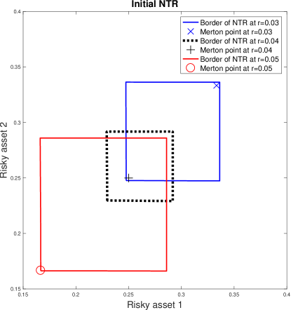
Figure A.1: NTRs with a stochastic interest rate.

A.2.2 Stochastic Volatility

Now we examine the case with stochastic volatility of risky returns, $\sigma_{t}=(\sigma_{t,1},\sigma_{t,2})^{\top}$. We assume that $\sigma_{t,1}$ and $\sigma_{t,2}$ are discrete Markov chains and independent of each other. Each $\sigma_{t,i}$ has two possible values: $0.16$ and 0.24, and its transition probability matrix is

$$\left[\begin{array}[]{cc}0.75&0.25\\ 0.25&0.75\end{array}\right]$$

for each $i=1,2$.

Figure A.2 displays the NTRs for four possible discrete states of $(\sigma_{t,1},\sigma_{t,2})$ at the initial time. The top-right polygon is the NTR for the state $(\sigma_{t,1},\sigma_{t,2})=(0.16,0.16)$, the bottom-left square is the NTR for the state $(\sigma_{t,1},\sigma_{t,2})=(0.24,0.24)$, and the top-left and the bottom-right squares are respectively the NTRs for the states $(\sigma_{t,1},\sigma_{t,2})=(0.24,0.16)$ and $(\sigma_{t,1},\sigma_{t,2})=(0.16,0.24)$. The mark, the diamond, the circle, and the plus are the corresponding Merton points if we assume that $(\sigma_{t,1},\sigma_{t,2})$ are fixed at their initial values. We see that a higher $\sigma_{t,i}$ implies a NTR and a Merton point closer to the origin of the coordinate system, consistent with the formula of the Merton point, (21). Moreover, when $(\sigma_{t,1},\sigma_{t,2})=(0.24,0.24)$, the no-shorting and/or no-borrowing constraints become binding for some portfolios before rebalancing. For example, if the portfolio before re-allocation is (0.5,0.5), the top-right vertex of the top-right polygon, then the optimal trading strategy is to keep the current portfolio unchanged (i.e., the no-borrowing constraint is binding).

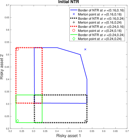
Figure A.2: NTRs with stochastic $\sigma$.

References

- [1] Abrams, R.A., and U.S. Karmarkar (1980). Optimal multiperiod investment-consumption policies. Econometrica, 48(2):333–353.
- [2] Akian, M., J.L. Menaldi, and A. Sulem (1996). On an investment-consumption model with transaction costs. SIAM Journal of Control and Optimization, 34(1):329–364.
- [3] Baccarin, S., and D. Marazzina (2014). Optimal Impulse Control of a Portfolio with a Fixed Transaction Cost. Central European Journal of Operations Research, vol. 22-2: 355–372.
- [4] Baccarin, S., and D. Marazzina (2016). Passive Portfolio Management over a Finite Horizon with a Target Liquidation Value under Transaction Costs and Solvency Constraints. IMA Journal of Management Mathematics, Vol. 27-4: 471–504.
- [5] Bellman, R. (1957). Dynamic Programming. Princeton University Press.
- [6] Black, F., and M. Scholes (1973). The pricing of options and corporate liabilities. Journal of Political Economy, 81(3):637–654.
- [7] Boyle, P.P., and X. Lin (1997). Optimal portfolio selection with transaction costs. North American Actuarial Journal, 1(2):27–39.
- [8] Brown, D.B., and J.E. Smith (2011). Dynamic portfolio optimization with transaction costs: heuristics and dual bounds. Management Science, 57(10):1752–1770.
- [9] Brumm, J., and S. Scheidegger (2017). Using Adaptive Sparse Grids to Solve High-Dimensional Dynamic Models. Econometrica, 85(5): 1575–1612.
- [10] Cai, Y. (2010). Dynamic Programming and Its Application in Economics and Finance. PhD thesis, Stanford University.
- [11] Cai, Y. (2019). Computational methods in environmental and resource economics. Annual Review of Resource Economics 11, 59–82.
- [12] Cai, Y., K.L. Judd, and T.S. Lontzek (2017). The social cost of carbon with economic and climate risks. Hoover economic working paper 18113.
- [13] Cai, Y., K.L. Judd, G. Thain, and S. Wright (2015). Solving dynamic programming problems on a computational grid. Computational Economics, 45(2), 261–284.
- [14] Cai, Y., and T.S. Lontzek (2019). The social cost of carbon with economic and climate risks. Journal of Political Economy, 127(6):2684–2734.
- [15] Constantinides, G.M. (1976). Optimal portfolio revision with proportional transaction costs: extension to HARA utility functions and exogenous deterministic income. Management Science, 22(8):921–923.
- [16] Constantinides, G.M. (1979). Multiperiod consumption and investment behavior with convex transaction costs. Management Science, 25:1127–1137.
- [17] Constantinides, G.M. (1986). Capital market equilibrium with transaction costs. Journal of Political Economy, 94(4):842–862.
- [18] Davis, M.H.A., and A.R. Norman (1990). Portfolio selection with transaction costs. Mathematics of Operations Research, 15(4):676–713.
- [19] Duffie, D., and T.S. Sun (1990). Transaction costs and portfolio choice in a discrete-continuous-time setting. Journal of Economic Dynamics and Control, 14:35–51.
- [20] Epstein, L.G., and S.E. Zin (1989). Substitution, risk-aversion, and the temporal behavior of consumption and asset returns: a theoretical framework. Econometrica, 57(4), 937–969.
- [21] Gennotte, G., and A. Jung (1994). Investment strategies under transaction costs: the finite horizon case. Management Science, 40(3):385–404.
- [22] Gill, P., W. Murray, M.A. Saunders and M.H. Wright (1994). User’s Guide for NPSOL 5.0: a Fortran Package for Nonlinear Programming. Technical report, SOL, Stanford University.
- [23] Goodman, J., and D.N. Ostrov (2010). Balancing small transaction costs with loss of optimal allocation in dynamic stock trading strategies. SIAM Journal of Applied Mathematics, 70(6):1977–1998.
- [24] Janecek, K., and S.E. Shreve (2004). Asymptotic analysis for optimal investment and consumption with transaction costs. Finance Stochast., 8(2):181–206.
- [25] Judd, K.L. (1998). Numerical Methods in Economics. The MIT Press.
- [26] Judd, K.L., L. Maliar, S. Maliar, and R. Valero (2014). Smolyak method for solving dynamic economic models: Lagrange interpolation, anisotropic grid and adaptive domain. Journal of Economic Dynamic and Control 44(C), 92–123.
- [27] Kamin, J.H. (1975). Optimal portfolio revision with a proportional transaction cost. Management Science, 21(11):1263–1271.
- [28] Liu, H. (2004). Optimal consumption and investment with transaction costs and multiple risky assets. Journal of Finance, 59:289–338.
- [29] Luenberger, D. (1997). Investment Science. Oxford University Press.
- [30] Malin, B., D. Krueger and F. Kubler (2011). Solving the Multi-Country Real Business Cycle Model using a Smolyak-Collocation Method. Journal of Economic Dynamics and Control, 35, 229–239.
- [31] Merton, R. (1969). Lifetime portfolio selection under uncertainty: the continuous time case. The Review of Economics and Statistics, 51(3):247–257.
- [32] Merton, R. (1971). Optimum consumption and portfolio rules in a continuous time model. Journal of Economic Theory, 3:373–413.
- [33] Muthuraman, K., and S. Kumar (2006). Multidimensional portfolio optimization with proportional transaction costs. Mathematical Finance, 16(2):301–335.
- [34] Muthuraman, K., and S. Kumar (2008). Solving free-boundary problems with applications in finance. Foundations and Trends in Stochastic Systems, 1(4):259–341.
- [35] Muthuraman, K., and H. Zha (2008). Simulation-based portfolio optimization for large portfolios with transaction costs. Mathematical Finance, 18(1):115–134.
- [36] Oksendal, B., and A. Sulem (2002). Optimal consumption and portfolio with both fixed and proportional costs. SIAM Journal on Control and Optimization, vol. 40: 1765–1790.
- [37] Rust, J. (2008). Dynamic Programming. In: New Palgrave Dictionary of Economics, ed. by Steven N. Durlauf and Lawrence E. Blume. Palgrave Macmillan, second edition.
- [38] Samuelson, P. (1969). Lifetime portfolio selection by dynamic stochastic programming. The Review of Economics and Statistics, 51(3):239–246.
- [39] Zabel, E. (1973). Consumer choice, portfolio decisions, and transaction costs. Econometrica, 41(2):321–335.

References

- [1] Cai, Y. (2010). Dynamic Programming and Its Application in Economics and Finance. PhD thesis, Stanford University.
- [2] Cai, Y. (2019). Computational methods in environmental and resource economics. Annual Review of Resource Economics 11, forthcoming. doi: 10.1146/annurev-resource-100518-093841.
- [3] Cai, Y., and K.L. Judd (2012). Dynamic programming with shape-preserving rational spline Hermite interpolation. Economics Letters, Vol. 117, No. 1, 161–164.
- [4] Cai, Y., and K.L. Judd (2013). Shape-preserving dynamic programming. Mathematical Methods of Operations Research, Vol. 77, No. 3, 407–421.
- [5] Cai, Y., and K.L. Judd (2015). Dynamic programming with Hermite approximation. Mathematical Methods of Operations Research, 81, 245–267.
- [6] Judd, K.L. (1998). Numerical Methods in Economics. The MIT Press.