Higgs portal to dark matter and $B\to K^{(*)}$ decays

Abstract

We consider a Higgs portal model in which the 125-GeV Higgs boson mixes with a light singlet mediator $h_{2}$ coupling to particles of a Dark Sector and study potential $b\to sh_{2}$ decays in the Belle II experiment. Multiplying the gauge-dependent off-shell Standard-Model $b$-$s$-Higgs vertex with the sine of the Higgs mixing angle does not give the correct $b$-$s$-$h_{2}$ vertex. We clarify this issue by calculating the $b$-$s$-$h_{2}$ vertex in an arbitrary $R_{\xi}$ gauge and demonstrate how the $\xi$ dependence cancels from physical decay rates involving an on-shell or off-shell $h_{2}$. Then we revisit the $b\to sh_{2}$ phenomenology and point out that a simultaneous study of $B\to K^{*}h_{2}$ and $B\to Kh_{2}$ helps to discriminate between the Higgs portal and alternative models of the Dark Sector. We further advocate for the use of the $h_{2}$ lifetime information contained in displaced-vertex data with $h_{2}$ decaying back to Standard-Model particles to better constrain the $h_{2}$ mass or to reveal additional $h_{2}$ decay modes into long-lived particles.

1 Introduction

The possibility of the Standard-Model (SM) Higgs field serving as the portal to dark matter Patt:2006fw has been extensively phenomenologically studied in the past two decades. A viable scenario involves a gauge singlet Higgs field which mixes with the SM Higgs field through appropriate terms in the Higgs potential, resulting in a dominantly SU(2)-doublet Higgs boson $h_{1}$ with mass 125 GeV and an additional Higgs boson $h_{2}$ with a priori arbitrary mass Schabinger:2005ei ; Greljo:2013wja ; Krnjaic:2015mbs . If the mixing angle is sufficiently small, the couplings of the 125-GeV Higgs $h_{1}$ comply with their SM values within the experimental error bars. The other Higgs boson $h_{2}$, which is mostly gauge singlet, serves as a mediator to the Dark Sector. In the simplest models the mediator couples to pairs of dark-matter (DM) particles. In this paper we are interested in the imprints of the described Higgs portal scenario on rare B meson decays which can be studied in the new Belle II experiment. If the $h_{2}$ mass is in the desired range below the $B$ mass, the decay of $h_{2}$ into a pair of DM particles must necessarily be kinematically forbidden to comply with the observed relic DM abundance Greljo:2013wja ; Krnjaic:2015mbs . Phenomenological studies of the scenario were recently performed in Refs. Krnjaic:2015mbs ; Winkler:2018qyg ; Matsumoto:2018acr ; Boiarska:2019jym ; Filimonova:2019tuy .

In this article we first revisit the calculation of the loop-induced amplitude $b\to sh_{2}$. The literature on the topic employs a result derived from the SM $\bar{s}b$-Higgs vertex with off-shell Higgs Batell:2009jf . However, it is known that this vertex is gauge-dependent Botella:1986gf . This observation calls for a novel calculation of the $\bar{s}bh_{2}$ vertex in an arbitrary $R_{\xi}$ gauge in order to investigate the correctness of the standard approach and to understand how the gauge parameter $\xi$ cancels in physical observables. After briefly reviewing the model in Sec. 2 we present our calculation of the $\bar{s}bh_{2}$ vertex in Sec. 3 and demonstrate the cancellation of the gauge dependence for the two cases with on-shell $h_{2}$ and an off-shell $h_{2}$ coupling to a fermion pair, respectively. In Sec. 4 we present a phenomenological analysis with several novel aspects, such as a study of the decay $B\to K^{*}h_{2}$ and a discussion of the lifetime information inferred from data on $B\to K^{(*)}h_{2}[\to f\bar{f}]$ with a displaced vertex of the $h_{2}$ decay into the fermion pair $f\bar{f}$. In Sec. 5 we conclude.

2 Model

A minimal extension of the SM with a real scalar singlet boson serving as mediator to the Dark Sector involves the Higgs potential:

$$V = V_{H}+V_{H\phi}+V_{\phi}+\text{h.c.}$$ (1)

$$\text{with}\qquad V_{H} = -\mu^{2}H^{\dagger}H+\frac{\bar{\lambda}_{0}}{4}(H^{\dagger}H)^{2},$$

$$V_{H\phi} = \frac{\alpha}{2}\phi(H^{\dagger}H),$$

$$V_{\phi} = \frac{m^{2}}{2}\phi^{2}+\frac{1}{4}\lambda_{\phi}\phi^{4},$$

where $\phi$ denotes the scalar singlet field in the interaction basis, while $H=\left(G^{+},(v+h+iG^{0})/\sqrt{2}\right)^{T}$ is the SM Higgs doublet. We minimize the scalar potential $V$ with respect to $\phi$ and $h$ and then choose to express the mass parameters $\mu$ and $m$ in terms of corresponding vacuum expectation values (vevs) $v_{\phi}$ and $v$, respectively:

$$\qquad\mu_{h}^{2} \equiv \frac{\partial^{2}V}{\partial h^{2}}\,=\,\frac{\bar{\lambda}_{0}v^{2}}{2},$$

$$\mu_{h\phi}^{2} \equiv \frac{\partial^{2}V}{\partial h\partial\phi}\,=\,\frac{\alpha v}{2},$$

$$\mu_{\phi}^{2} \equiv \frac{\partial^{2}V}{\partial\phi^{2}}\,=\,2\lambda_{\phi}v_{\phi}^{2}-\frac{\alpha v^{2}}{4v_{\phi}}\,.$$ (2)

The corresponding off-diagonal mass matrix is diagonalized with the introduction of the mixing angle $\theta$

$$\quad h=\cos\theta\,h_{1}-\sin\theta\,h_{2},\quad\phi=\sin\theta\,h_{1}+\cos\theta\,h_{2}\,.$$ (3)

As mentioned in the introduction, we choose $h_{2}$ as the light mass eigenstate, whose signatures we are primarily interested in, while $h_{1}$ corresponds to the observed Higgs boson with mass $125\,\text{GeV}$.

An important Feynman rule for the calculation of the scalar penguin in $R_{\xi}$ gauge is the one for the $G^{+}G^{-}h_{2}$ vertex. After diagonalization the mass matrix we find

$$\qquad G^{+}G^{-}h_{1}:\enskip\quad-i\frac{em_{h_{1}}^{2}\cos\theta}{2m_{W}\sin\theta_{W}},$$

$$\qquad G^{+}G^{-}h_{2}:\enskip\quad\phantom{-}i\frac{em_{h_{2}}^{2}\sin\theta}{2m_{W}\sin\theta_{W}}.$$ (4)

One easily verifies that the rest of the vertices that are required for the studies of low energy phenomenology are simple rescalings of the corresponding SM Higgs vertices by the factor $(-\sin\theta)$. Note that the $G^{+}G^{-}h_{2}$ vertex is not found in the same way from the corresponding SM vertex, but in addition involves the proper replacement of the SM Higgs mass by $m_{h_{2}}$.

One could have included more terms in the scalar potential in Eq. (1) such as $\phi^{2}H^{\dagger}H$, however, such terms would not change the low-energy phenomenology related to the process of our interest but would merely influence the scalar self-interactions that we are currently not concerned with.

3 The $\bar{s}bh_{2}$ vertex in the $R_{\xi}$ gauge

We employ a general $R_{\xi}$ gauge for the calculation of the Feynman diagrams contributing to the $\bar{s}\text{-}b\text{-}h_{2}$ vertex. We further use the FeynArts package Hahn:2000kx for generating the amplitudes and the FeynCalc Mertig:1990an ; Shtabovenko:2016sxi ; Shtabovenko:2020gxv , Package-X Patel:2015tea , and FeynHelpers Shtabovenko:2016whf packages to evaluate the analytic expressions for the Feynman diagrams. Neglecting the mass of the external $s$ quark, we encounter the diagrams shown in Fig. 1. In our final result we will also neglect the masses of the internal up and charm quarks. While the expressions for individual diagrams contain ultraviolet poles, the final result is UV convergent due to the Glashow-Iliopoulos-Maiani mechanism.

(a) t

(b) t

(c) t

(d) t

(e) t

(f) t

(g) t

(h) t

Figure 1: One-loop diagrams contributing to $b\to sh_{2}$ in $R_{\xi}$ gauge.

 

In order to elucidate the gauge independence of the physical quantities, we set the $h_{2}$ boson off the mass shell. In a first step we present the results in terms of the scalar loop functions $B_{0},C_{0}$ of the Passarino-Veltman (PV) basis, keeping exact dependences on all momenta and masses. For the final goal to calculate the low-energy Wilson coefficient governing the decay process $b\to s\ h_{2}$ this appears unnecessary, but it turns out that the expression in terms of the PV basis is compact and most suitable for studying the gauge-independence of the physical quantities.

We decompose each diagram $\mathcal{A}_{i}$ as $\mathcal{A}_{i}=\tilde{\mathcal{A}}_{i}+\mathcal{A}_{i}^{(\xi)}$, with the second term $\mathcal{A}_{i}^{(\xi)}$ comprising all terms which depend on the $W$ gauge parameter $\xi$. The expressions for $\tilde{\mathcal{A}}_{i}$ are collected in A. The results for the gauge-dependent pieces of the individual diagrams are rather lengthy, so we only provide the total sum

$$\;\sum_{i}\mathcal{A}_{i}^{(\xi)} = \sin\theta\dfrac{m_{b}m_{t}^{2}}{8\pi^{2}v^{3}(m_{b}^{2}-p_{h_{2}}^{2})}(p_{h_{2}}^{2}-m_{h_{2}}^{2})\cdot$$ (5)

$$\!\!\!\bigg{[}B_{0}(p_{h_{2}}^{2},m_{W}^{2}\xi,m_{W}^{2}\xi)-B_{0}(m_{b}^{2},m_{t}^{2},m_{W}^{2}\xi)$$

$$\quad+\,(p_{h_{2}}^{2}-m_{b}^{2}+m_{t}^{2}-m_{W}^{2}\xi)\cdot$$

$$\qquad C_{0}(0,m_{b}^{2},p_{h_{2}}^{2},m_{W}^{2}\xi\,,m_{t}^{2},m_{W}^{2}\xi)\bigg{]}\,,$$

with $\lambda_{t}=V_{tb}V^{\ast}_{ts}$. Here and in the following we suppress the Dirac spinors for the $b$ and $s$ quarks. It follows from the expression above that the gauge-dependent contribution $\mathcal{A}^{(\xi)}$ vanishes for the case of an on-shell scalar boson, which confirms the gauge independence of the corresponding physical on-shell amplitude. We write the total $\bar{s}bh_{2}$ vertex $\mathcal{A}=\sum_{i}(\tilde{\mathcal{A}}_{i}+\mathcal{A}_{i}^{(\xi)})$ (with on-shell quarks and off-shell $h_{2}$) as

$$\mathcal{A}=G(p_{h_{2}}^{2},m_{h_{2}}^{2})+(p_{h_{2}}^{2}-m_{h_{2}}^{2})F(\xi,p_{h_{2}}^{2}),$$ (6)

with the second term equal to the expression in Eq. (5). We note that $F(\xi,p_{h_{2}}^{2})$ does not depend on $m_{h_{2}}$. While the cancellation of $\xi$ from $\mathcal{A}$ is obvious for an on-shell $h_{2}$, i.e. for the decay $b\to s\ h_{2}$, this feature is not immediately transparent for the case in which an off-shell $h_{2}$ decays into a pair of other particles. In such scenarios the gauge dependence is cancelled by other diagrams. Here we exemplify the cancellation of the gauge parameter for a model in which our mediator $h_{2}$ couples to a pair of invisible final state fermions:

$$\qquad\mathcal{L}_{\phi\chi\chi}\;=\;\lambda_{\chi}\phi\overline{\chi}\chi\,,$$ (7)

meaning that $h_{2}$ in $b\to s\ h_{2}[\to\overline{\chi}\chi]$ is necessarily off-shell Krnjaic:2015mbs . In order to find the cancellation of the gauge parameter we must also consider the diagrams corresponding to $b\to s\ h_{1}[\to\overline{\chi}\chi]$ involving the heavy SM-like state $h_{1}$. The amplitudes involving the $h_{2}$ and $h_{1}$ propagators are proportional to $-\sin\theta$ and to $\cos\theta$, respectively:

$$\begin{split}\qquad\mathcal{A}_{b\text{-}s\text{-}h2}\sim-\sin\theta,\qquad\qquad\mathcal{A}_{b\text{-}s\text{-}h1}\sim\cos\theta,\end{split}$$ (8)

while the vertices $\mathcal{V}_{h_{1,2}\chi\chi}$ involving the coupling of the dark-matter fermion to the scalar bosons depend on $\theta$ as $\mathcal{V}_{h_{1}\chi\chi}\sim\sin\theta$ and $\mathcal{V}_{h_{2}\chi\chi}\sim\cos\theta$. The $b\to s\ h_{1,2}[\to\overline{\chi}\chi]$ amplitudes $\mathcal{A}_{h_{1,2}}$ can be schematically written as

$$\quad\mathcal{A}_{h_{2}} = -\lambda_{\chi}\sin\theta\cos\theta\left(F(\xi,p^{2})+\frac{G(p^{2},m_{h_{2}}^{2})}{p^{2}-m_{h_{2}}^{2}}\right),$$ (9)

$$\quad\mathcal{A}_{h_{1}} = \phantom{-}\lambda_{\chi}\sin\theta\cos\theta\left(F(\xi,p^{2})+\frac{G(p^{2},m_{h_{1}}^{2})}{p^{2}-m_{h_{1}}^{2}}\right),$$ (10)

where $p^{2}$ denotes the square of the momentum transferred to the fermion pair. By adding the two amplitudes one verifies the cancellation of the gauge-dependent part $F(\xi,p^{2})$. If one considers processes with off-shell $h_{1,2}$ exchange to SM fermions, such as in $b\to s\tau^{+}\tau^{-}$ with e.g. $m_{h_{2}}>m_{b}$, also box diagrams are needed for the proper gauge cancellation as found in Ref. Botella:1986gf for the SM case.

We now proceed to integrate out the top quark and W boson within the gauge independent contribution $\tilde{\mathcal{A}}\equiv\sum_{i}\tilde{\mathcal{A}}_{i}$ to obtain the Wilson coefficient:

$$\mathcal{L}_{\text{eff}} = C_{h_{2}sb}\,h_{2}\,\overline{s}P_{R}b+\text{h.c.},$$ (11)

$$\qquad\qquad C_{h_{2}sb} = -\frac{3\,\sin\theta\,\lambda_{t}\,m_{b}\,m_{t}^{2}}{16\,\pi^{2}\,v^{3}}\,,$$ (12)

where $v\simeq 246\,\text{GeV}$ is the vacuum expectation value of the Higgs doublet. This result agrees with Ref. Winkler:2018qyg , whereas it agrees with Refs. Krnjaic:2015mbs and Batell:2009jf up to the sign.

The procedure to multiply the SM result for the $\bar{s}b$-Higgs vertex by $-\sin\theta$ to find the $\bar{s}bh_{2}$ vertex is not correct in an $R_{\xi}$ gauge (nor for the special cases $\xi=0$ or $\xi=1$ of the Landau and ’t Hooft-Feynman gauges) because of the subtlety with the $G^{\pm}$ vertices in Eq. (4). However, the missing terms are suppressed by higher powers of $m_{h_{2}}^{2}/M_{W}^{2}$ and do not contribute to the effective dimension-4 lagrangian in Eq. (11).

Figure 2: Comparison of the branching fractions of $B^{+}\to K^{+}h_{2}$ (thick orange curve) and $B^{+}\to K^{\ast+}h_{2}$ (dashed purple curve) for $\sin\theta=10^{-4}$.

 

4 Phenomenology

The experimental signature $B\to K\,h_{2}$ permits the determination of $m_{h_{2}}$ from the decay kinematics, while the other relevant parameter of the model, $\sin\theta$, can be determined from the measured branching ratio $B(B\to K\,h_{2})$. With increasing $m_{h_{2}}$ more $h_{2}$ decay channels open and the $h_{2}$ lifetime may be in a favourable range allowing the $h_{2}$ to decay within the Belle II detector. This scenario has a characteristic displaced-vertex signature which is highly beneficial for the experimental analysis. Higgs-portal signatures at $B$ factories have been widely studied Krnjaic:2015mbs ; Winkler:2018qyg ; Filimonova:2019tuy ; Kamenik:2011vy ; Schmidt-Hoberg:2013hba ; Clarke:2013aya ; Sierra:2015fma . In this paper we briefly revisit the recent analyses of Refs. Winkler:2018qyg ; Filimonova:2019tuy and complement them with novel elements: Firstly, we present a novel analysis of the decay mode $B\to K^{*}(892)h_{2}$ in comparison to $B\to Kh_{2}$. Secondly, we highlight the benefits of the lifetime information which can be obtained from the displaced-vertex data. Thirdly, we present a new result of the number of $B\to Kh_{2}[\to f]$ events (with $f$ representing a pair of light particles) expected at Belle II as a function of the relevant $B\to Kh_{2}$ and $h_{2}\to f$ branching ratios.

In our study of $B\to Kh_{2}$ and $B\to K^{\ast}h_{2}$ with subsequent decay of $h_{2}$ into a visible final states with displaced vertex we restrict ourselves to the case $m_{h_{2}}>2m_{\mu}$. While the leptonic decay rate is given by the simple formula

$$\quad\Gamma(h_{2}\to\ell\ell)=\sin^{2}\theta\frac{G_{F}m_{h_{2}}m_{\ell}^{2}}{4\sqrt{2}\pi}\bigg{(}1-\frac{4m_{\ell}^{2}}{m_{h_{2}}^{2}}\bigg{)}^{3/2}\,,$$ (13)

the calculation of the decay rate into an exclusive hadronic final state is challenging. Different calculations of $\Gamma(h_{2}\to\pi\pi)$ and $\Gamma(h_{2}\to KK)$ Voloshin:1985tc ; Truong:1989my ; Donoghue:1990xh ; Monin:2018lee employing chiral perturbation theory have been clarified, updated and refined in Ref. Winkler:2018qyg and we use the results of this reference. In the region with $m_{h_{2}}>2\,\text{GeV}$ the inclusive hadronic decay rate can be reliably calculated in perturbation theory Grinstein:1988yu .

Analyses with fully visible final states $K^{(\ast)}f$ can also be done at LHCb Aaij:2016qsm ; Aaij:2015tna .

4.1 $B\to Kh_{2}$

The branching ratio of $B\to Kh_{2}$ is

$$\;B(B\to Kh_{2})=\frac{\tau_{B}}{32\pi m_{B}^{2}}|C_{h_{2}sb}|^{2}\bigg{(}\frac{m_{B}^{2}-m_{K}^{2}}{m_{b}-m_{s}}\bigg{)}^{2}\cdot$$

$$f_{0}(m_{h_{2}}^{2})^{2}\frac{\lambda(m_{B}^{2},m_{K}^{2},m_{h_{2}}^{2})^{1/2}}{2m_{B}}\,,$$ (14)

where $\lambda(a,b,c)=a^{2}+b^{2}+c^{2}-2(ab+ac+bc)$, and the scalar form factor $f_{0}(q^{2})$ is related to the desired scalar hadronic matrix element as

$$\qquad\langle K|\bar{s}b|B\rangle=\frac{m_{B}^{2}-m_{K}^{2}}{m_{b}-m_{s}}\,f_{0}(q^{2})\,,$$ (15)

where $q=p_{B}-p_{K}$. For this form factor we use the QCD lattice result of Ref. Bailey:2015dka (see also Bouchard:2013pna ).

The reach of the Belle II experiment for the process $B\to Kh_{2}$ was recently studied in Ref.Filimonova:2019tuy . This investigation involves a study of the detector geometry and we present a novel study in B. For the evaluation of the number of events we use the formula (40). Our evaluation of the sensitivities corresponds to $5\cdot 10^{10}$ produced $B\bar{B}$ meson pairs, where $B$ represents both $B^{+}$ and $B^{0}$, at $50\,\text{ab}^{-1}$ of data at Belle II experiment Kou:2018nap .

The parameter regions that correspond to three or more displaced vertex events of any of the final state signatures in $B\to K(h_{2}\to f)$, $f=(\pi\pi+KK),\mu\mu,\tau\tau$ within the Belle II detector are displayed by the dashed red contours in figure 3. The number of events involve the summation over the decays of $B^{+}$, $B^{0}$ and the corresponding charge-conjugate mesons. Following Ref. Filimonova:2019tuy , we display the regions in which the $\pi\pi,KK$ final states occur as well as the region above the $\tau$ lepton threshold within the same plot. We show the contours of the proper lifetime of the scalar mediator within the same parameter space and encourage our experimental colleagues to include the lifetime information in the following ways: In a first step one may assume the minimal model adopted in this paper and use the lifetime measurements as additional information on $m_{h_{2}}$ and $\sin\theta$. E.g. if $h_{2}$ is light enough so that the only relevant decay channel is $h_{2}\to\mu^{+}\mu^{-}$, the lifetime is the inverse of the width in Eq. (13). Thanks to the strong dependence on $m_{h_{2}}$ the lifetime information will improve the determination of $m_{h_{2}}$ inferred from the $B\to Kh_{2}$ decay kinematics once $\sin\theta$ is fixed from branching ratios. With more statistics one can go a step further and use the lifetime information to verify or falsify the model. Even if all $h_{2}$ couplings to SM particles originate from the SM Higgs field through mixing, a richer singlet scalar sector can change the $h_{2}$ lifetime. Consider an extra gauge singlet scalar field $\tilde{\phi}$ coupling to $\phi$ in the potential in Eq. (1) giving rise to a third physical Higgs state $h_{3}$. If $h_{3}$ is sufficiently light, $h_{2}\to h_{3}h_{3}$ is possible. Through $\tilde{\phi}$–$H$ mixing the new particle $h_{3}$ will decay back into SM particles, but the lifetime can be so large that $h_{2}\to h_{3}h_{3}$ is just a missing-energy signature. Then the only detectable effect of the extra $h_{2}\to h_{3}h_{3}$ mode is a shorter $h_{2}$ lifetime. If measured precisely enough, the lifetime will permit to determine the decay rate of $h_{2}\to h_{3}h_{3}$ and thereby the associated coupling constant. Alternatively, one may fathom a model in which $h_{2}$ decays into a pair of sterile neutrinos which decay back to SM fermions.

 

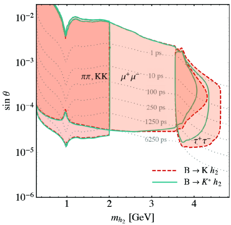
Figure 3: Parameter regions that correcpond to three or more events of $B\to Kh_{2}\,(\to f)$, $f=(\pi\pi+KK),\mu^{+}\mu^{-},\tau^{+}\tau^{-}$ are shaded in red and bounded by the dashed red contours. Analogous regions for $B\to K^{\ast}h_{2}$ are presented by the dark green contour. We summed over the number of events in the decays of $B^{+}$, $B^{-}$, $B^{0}$, and $\bar{B}^{0}$. The dotted lines are contours of constant $h_{2}$ proper lifetime.

 

4.2 $B\to K^{\ast}h_{2}$

We include in our analysis the decay of $B$ meson that involves the final state vector meson $K^{\ast}$ and has the branching fraction

$$\quad B(B\to K^{\ast}h_{2}) = \frac{\tau_{B}}{32\pi m_{B}^{2}}|C_{h_{2}sb}|^{2}\frac{A_{0}(m_{h_{2}}^{2})^{2}}{(m_{b}+m_{s})^{2}}\cdot$$ (16)

$$\quad\frac{\lambda(m_{B}^{2},m_{K^{\ast}}^{2},m_{h_{2}}^{2})^{3/2}}{2m_{B}}\,.$$

The form factor $A_{0}(q^{2})$ is related to the desired pseudoscalar hadronic matrix element as

$$\langle K^{\ast}(k,\epsilon)|\bar{s}\gamma_{5}b|B(p_{B})\rangle=\frac{2\,m_{K^{\ast}}\,\epsilon^{\ast}\cdot q}{m_{b}+m_{s}}A_{0}(q^{2})\,,$$ (17)

where $\epsilon$ is a polarization vector of $K^{\ast}$ and $q=p_{B}-k$. For this form factor we use the combination of results from lattice QCD Horgan:2013hoa and QCD sum rules Straub:2015ica as provided in Ref. Straub:2015ica .

$B(B\to K^{\ast}h_{2})$ is comparable in size to $B(B\to Kh_{2})$ for masses up to $\sim 2\,\text{GeV}$ (see Fig. 2), and is suppressed as the mass $m_{h_{2}}$ approaches the kinematic endpoint. This is the result of the additional power of the kinematic function $\lambda$ in Eq. (16) that comes from the contribution of the longitudinal $K^{\ast}$ polarization. It follows from angular momentum conservation that this is the only contributing polarization. The combination of the experimental data from both processes will be required in order to discriminate the spin-0 vs. spin-1 hypotheses in case of a discovery. E.g. the mediator with spin 1 involves a different dependence of the rate on the mediator’s mass and comes with a dramatic suppression of the decay rate with $K$ in the final state if the mediator is light. The decay $B\to K^{\ast}h_{2}$ has been studied before in Ref. Boiarska:2019jym , in which a plot similar to our Fig. 2 is presented for the sum of several vector resonances. Our analysis of Belle II opportunities is new compared to Ref. Boiarska:2019jym which focuses on LHC, ShiP, and DUNE. Refs. Boiarska:2019jym ; Filimonova:2019tuy further study the fully inclusive decay $B\to X_{s}h_{2}$.

The kinematic suppression close to the endpoint implies that the number of $B\to K^{\ast}h_{2}(\tau\tau)$ events will be much smaller relative to the case of the final state with $K$. We display the corresponding parameter region corresponding to $K^{\ast}$ events with the dark green contour in Fig. 3.

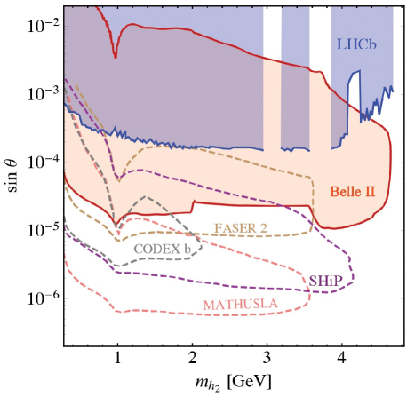
Figure 4: Combined sensitivity of the Belle II experiment to displaced vertices of $h_{2}$ including both $B\to Kh_{2}$ and $B\to K^{\ast}h_{2}$ and decays of $h_{2}$ to $(\pi\pi+KK),\mu^{+}\mu^{-},\tau^{+}\tau^{-}$ are shown with the filled red region, and compared to the search limit of LHCb Aaij:2016qsm (shaded blue) and projected sensitivities by other proposed experiments, Mathusla Evans:2017lvd (pink), SHiP Alekhin:2015byh , CODEX b Gligorov:2017nwh (gray) and FASER 2 Ariga:2018uku (brown).

 

In Fig. 4 we compare the reach of the Belle II experiment to displaced vertices of $h_{2}$ including both $B\to Kh_{2}$ and $B\to K^{\ast}h_{2}$ processes and decays of $h_{2}$ to $(\pi\pi+KK),\mu^{+}\mu^{-},\tau^{+}\tau^{-}$ with the existing search limit of the LHCb experiment Aaij:2016qsm . We also compare to projected sensitivities of other proposed experiments, Mathusla Evans:2017lvd , SHiP Alekhin:2015byh , CODEX b Gligorov:2017nwh and FASER 2 Ariga:2018uku .

5 Conclusions

We have clarified the cancellation of gauge-dependent terms appearing in the $\bar{s}bh_{2}$ vertex in the standard Higgs portal model with a singlet mediator to the Dark Sector. We have further updated the $b\to sh_{2}$ phenomenology to be studied at the Belle II detector, with a novel consideration of $B\to K^{*}h_{2}$ complementing the previously studied decay $B\to Kh_{2}$. Decays like $B\to K^{(*)}h_{2}[\to\mu^{+}\mu^{-}]$ with a displaced vertex permit the measurement of the $h_{2}$ lifetime. It is shown how this measurement will further constrain the two relevant parameters $m_{h_{2}}$ and $\sin\theta$ of the model. Both the lifetime information and the combined study of $B\to K^{*}h_{2}$ and $B\to Kh_{2}$ permit the discrimination of the studied Higgs portal from other Dark-Sector models. Another result of this paper is a new calculation of the expected number of $B\to K^{*}h_{2}[\to f]$ events as a function of the $B\to Kh_{2}$ and $h_{2}\to f$ branching ratios for the Belle II detector.

Appendix A Results of the loop calculation

In this appendix we present the results for the $\xi$-independent pieces $\tilde{\mathcal{A}}_{i}$ corresponding to the individual Feynman diagrams shown in Fig. 1:

$$\tilde{\mathcal{A}}_{(a)}=-\sin\theta\,\dfrac{\lambda_{t}\,m_{b}m_{t}^{2}}{8\pi^{2}v^{3}}\frac{p_{h_{2}}^{2}-2m_{t}^{2}}{m_{b}^{2}-p_{h_{2}}^{2}}\,B_{0}(p_{h_{2}}^{2},m_{t}^{2},m_{t}^{2})\,$$

$$\tilde{\mathcal{A}}_{(b)} =0\,,$$ (18)

$$\tilde{\mathcal{A}}_{(c)}= -\sin\theta\dfrac{\lambda_{t}\,m_{t}^{2}}{16\,\pi^{2}\,m_{b}v^{3}}\dfrac{1}{m_{b}^{2}-p_{h_{2}}^{2}}\cdot$$

$$\bigg{\{}\big{[}-m_{b}^{2}\big{(}m_{W}^{2}(4D+5x-9)+p_{h_{2}}^{2}\big{)}+3m_{b}^{4}$$

$$+m_{W}^{2}p_{h_{2}}^{2}(x-1)\big{]}B_{0}(m_{b}^{2},m_{t}^{2},m_{W}^{2})$$

$$+2m_{b}^{2}m_{W}^{2}\big{(}m_{b}^{2}(2-x)+2m_{W}^{2}(x-1)(2+x)$$

$$-p_{h_{2}}^{2}\big{)}C_{0}(0,m_{b}^{2},p_{h_{2}}^{2},m_{t}^{2},m_{W}^{2},m_{t}^{2})$$

$$-4(D-2)m_{b}^{2}m_{W}^{2}B_{0}(p_{h_{2}}^{2},m_{t}^{2},m_{t}^{2})$$

$$+\dfrac{2m_{W}^{2}(m_{b}^{2}-p_{h_{2}}^{2})}{D-2}B_{0}(0,m_{W}^{2},m_{W}^{2})\bigg{\}}\,,$$ (19)

$$\tilde{\mathcal{A}}_{(d)}= -\sin\theta\dfrac{\lambda_{t}\,m_{b}}{8\pi^{2}v^{3}}\big{(}(m_{t}^{2}-2m_{W}^{2})B_{0}(0,m_{t}^{2},m_{W}^{2})$$

$$+2m_{W}^{2}B_{0}(0,0,m_{W}^{2})\big{)}\,,$$ (20)

$$\tilde{\mathcal{A}}_{(e)}= \sin\theta\,\dfrac{\lambda_{t}\,m_{t}^{2}}{16\pi^{2}(D-2)m_{b}v^{3}(m_{b}^{2}-p_{h_{2}}^{2})}\cdot$$

$$\big{[}2m_{W}^{2}(m_{b}^{2}-p_{h_{2}}^{2})B_{0}(0,m_{W}^{2},m_{W}^{2})$$ (21)

$$-(D-2)\big{(}m_{b}^{4}-m_{b}^{2}(m_{t}^{2}+m_{W}^{2}+3p_{h_{2}}^{2})$$

$$+p_{h_{2}}^{2}(m_{t}^{2}-m_{W}^{2})\big{)}B_{0}(m_{b}^{2},m_{t}^{2},m_{W}^{2})\big{]}\,,$$

$$\tilde{\mathcal{A}}_{(f)}= -\sin\theta\,\dfrac{\lambda_{t}\,m_{b}}{8\pi^{2}\,v^{3}(m_{b}^{2}-p_{h_{2}}^{2})}\,\Big{\{}m_{W}^{2}\big{(}2(2-D)m_{W}^{2}$$

$$+2m_{b}^{2}-m_{t}^{2}\big{)}B_{0}(m_{b}^{2},m_{t}^{2},m_{W}^{2})$$

$$-2m_{W}^{2}\big{(}m_{b}^{2}-(D-2)m_{W}^{2}\big{)}B_{0}(m_{b}^{2},0,m_{W}^{2})$$

$$+m_{t}^{2}(2m_{W}^{2}+p_{h_{2}}^{2})B_{0}(p_{h_{2}}^{2},m_{W}^{2},m_{W}^{2})$$

$$+\big{[}m_{t}^{2}(2m_{W}^{4}-m_{W}^{2}p_{h_{2}}^{2}+p_{h_{2}}^{4})$$

$$-4m_{W}^{6}+2m_{b}^{4}m_{W}^{2}-m_{b}^{2}\big{(}m_{t}^{2}(2m_{W}^{2}+p_{h_{2}}^{2})$$

$$+2m_{W}^{2}p_{h_{2}}^{2}\big{)}+m_{t}^{4}(2m_{W}^{2}+p_{h_{2}}^{2})$$

$$+2m_{W}^{4}p_{h_{2}}^{2}\big{]}C_{0}(0,m_{b}^{2},p_{h_{2}}^{2},m_{W}^{2},m_{t}^{2},m_{W}^{2})$$

$$-2m_{W}^{2}(-2m_{W}^{4}+m_{b}^{4}-m_{b}^{2}p_{h_{2}}^{2}$$

$$+m_{W}^{2}p_{h_{2}}^{2})C_{0}(0,m_{b}^{2},p_{h_{2}}^{2},m_{W}^{2},0,m_{W}^{2})\Big{\}}\,,$$ (22)

$$\tilde{\mathcal{A}}_{(g)} =-\sin\theta\,\frac{\lambda_{t}m_{t}^{4}}{4\,\pi^{2}(D-2)m_{b}v^{3}}B_{0}(0,m_{t}^{2},m_{t}^{2})\,,$$ (23)

$$\tilde{\mathcal{A}}_{(h)}= \sin\theta\,\dfrac{\lambda_{t}\,m_{W}^{2}}{8\,\pi^{2}m_{b}v^{3}}\cdot$$

$$\Big{[}m_{W}^{2}(x-1)(D+x-2)B_{0}(0,m_{t}^{2},m_{W}^{2})$$

$$+\dfrac{2\,m_{t}^{2}}{D-2}\,B_{0}(0,m_{W}^{2},m_{W}^{2})$$

$$+(D-2)\,m_{W}^{2}B_{0}(0,0,m_{W}^{2})$$

$$-2\,m_{t}^{2}B_{0}(0,m_{t}^{2},m_{t}^{2})\Big{]}\,,$$ (24)

where $\lambda_{t}=V_{tb}\,V_{ts}^{\ast}$, $x=m_{t}^{2}/m_{W}^{2}$ and $D=4-2\epsilon$. The above results are to be multiplied with $\bar{s}P_{R}b$, where $s$ and $b$ denote the appropriate spinors and $P_{R}\equiv(1+\gamma_{5})/2$.

Our definitions of Passarino-Veltman loop functions follow the Feyncalc package Mertig:1990an ; Shtabovenko:2016sxi ; Shtabovenko:2020gxv :

$$i\pi^{2}B_{0}(p_{1}^{2},m_{1}^{2},m_{2}^{2})$$

$$=\int d^{D}k\frac{1}{(k^{2}-m_{1}^{2})\left((k+p_{1})^{2}-m_{2}^{2}\right)}\,,$$ (25)

$$i\pi^{2}C_{0}(p_{1}^{2},(p_{1}-p_{2})^{2},p_{2}^{2},m_{1}^{2},m_{2}^{2},m_{3}^{2})$$ (26)

$$=\int d^{D}k\frac{1}{(k^{2}-m_{1}^{2})\left((k+p_{1})^{2}-m_{2}^{2}\right)\left((k+p_{2})^{2}-m_{3}^{2}\right)}\,.$$

Appendix B Evaluation of the number of events at Belle II

We describe the formula for the evaluation of the number of events in $B\to K^{(\ast)}h_{2}$, with the long-lived scalar $h_{2}$ decaying back to $f$, a pair of leptons or hadrons at Belle II.

The energy and the magnitude of the momentum of $h_{2}$ in the $B$ meson rest-frame are:

$$E_{h_{2}}=\dfrac{m_{B}^{2}+m_{h_{2}}^{2}-m_{K^{(\ast)}}^{2}}{2m_{B}}\,,\quad|\vec{p}_{h_{2}}|=\sqrt{E_{h_{2}}^{2}-m_{h_{2}}^{2}}\,.$$ (27)

For our coordinate system we choose the $z$-axis in the direction of the electron beam. The convention for the angle $\vartheta$ follows Chapter 3 of Ref. Kou:2018nap . We consider the Lorentz transformation from the rest frame $h_{2}$ to the laboratory frame, $\mathcal{B}_{1}\mathcal{R}\mathcal{B}_{0}$, where $\mathcal{R}\mathcal{B}_{0}$ is the transformation from the rest frame of $h_{2}$ to the rest frame of the $B$ meson:

$$\qquad\mathcal{R}\mathcal{B}_{0}\begin{pmatrix}m_{h_{2}}\\ 0\\ 0\\ 0\end{pmatrix}=\begin{pmatrix}E_{h_{2}}\\ 0\\ |\vec{p}_{h_{2}}|\sin\vartheta_{0}\\ |\vec{p}_{h_{2}}|\cos\vartheta_{0}\end{pmatrix}\,,$$ (28)

and $\mathcal{B}_{1}$ is the boost from the $\Upsilon$ rest frame to the laboratory frame. The $B$ meson pair is produced nearly at rest in the decay of the $\Upsilon$ resonance, so we neglect a small Lorentz boost from the $\Upsilon$ rest frame to the B rest frame. We also conveniently set the azimuthal angle $\phi$ to zero since it is not affected by the $\mathcal{B}_{1}$ boost along the $z$ direction. The latter boost is induced by the asymmetric beam energies $E_{-}=7\,\text{GeV}$ and $E_{+}=4\,\text{GeV}$ of electrons and positrons, respectively, and is determined by $\beta_{B}\gamma_{B}=(E_{-}-E_{+})/2(E_{-}E_{+})^{1/2}=0.28$, $\gamma_{B}=1.04$.

In the rest frame of the mediator, the decay occurs at $(c\tau,0,0,0)$. The decay length in the laboratory frame follows from

$$\begin{pmatrix}ct_{\text{lab}}\\ x_{\text{lab}}\\ y_{\text{lab}}\\ z_{\text{lab}}\end{pmatrix}\,=\mathcal{B}_{1}\mathcal{R}\mathcal{B}_{0}\begin{pmatrix}c\tau\\ 0\\ 0\\ 0\end{pmatrix}$$

$$=\frac{c\tau}{m_{h_{2}}}\begin{pmatrix}\gamma_{B}&0&0&\gamma_{B}\beta_{B}\\ 0&1&0&0\\ 0&0&1&0\\ \gamma_{B}\beta_{B}&0&0&\gamma_{B}\end{pmatrix}\begin{pmatrix}E_{h_{2}}\\ 0\\ |\vec{p}_{h_{2}}|\sin\vartheta_{0}\\ |\vec{p}_{h_{2}}|\cos\vartheta_{0}\end{pmatrix}$$ (29)

$$=\frac{c\tau}{m_{h_{2}}}\begin{pmatrix}\gamma_{B}E_{h_{2}}+\gamma_{B}\beta_{B}|\vec{p}_{h_{2}}|\cos\vartheta_{0}\\ 0\\ |\vec{p}_{h_{2}}|\sin\vartheta_{0}\\ \gamma_{B}\beta_{B}E_{h_{2}}+\gamma_{B}|\vec{p}_{h_{2}}|\cos\vartheta_{0}\end{pmatrix}\,.$$

The decay length of the mediator in the laboratory frame is $d_{L}=(x_{\text{lab}}^{2}+y_{\text{lab}}^{2}+z_{\text{lab}}^{2})^{1/2}$ and is related to the corresponding angle $\theta$ as

$$y_{\text{lab}}=d_{L}(\theta_{0})\sin\vartheta,\quad z_{\text{lab}}=d_{L}(\theta_{0})\cos\vartheta\,.$$ (30)

The expected number of $B^{\pm}\to K^{(\ast)\pm}h_{2}[\to f]$ events is

$$\quad N^{\pm}_{f} =N_{B^{+}B^{-}}\cdot 2\cdot B(B^{\pm}\to K^{(\ast)\pm}h_{2})B(h_{2}\to f)\cdot$$ (31)

$$\quad\int d\vartheta\,p(\vartheta)\frac{1}{d_{L}}\int_{r_{\text{min}}(\vartheta)}^{r_{\text{max}}(\vartheta)}dre^{-\frac{r}{d_{L}}}\,,$$

where $N_{B^{+}B^{-}}$ is the total number of produced $B^{+}\text{-}B^{-}$ meson pairs. We include the differences in the lifetimes and the production asymmetry of $B^{+}$ and $B^{0}$ mesons:

$$\tau_{B^{+}}=1.638\,\text{ps}\,,\qquad\tau_{B^{0}}=1.519\,\text{ps}\,,$$ (32)

$$f^{+-}\equiv B(\Upsilon(4S)\to B^{+}B^{-})=0.514\,,$$ (33)

$$f^{00}\equiv B(\Upsilon(4S)\to B^{0}\bar{B}^{0})=0.486\,,$$ (34)

where the numerical values are taken from Amhis:2019ckw . The total number of the displaced vertex events, summed over the decays of $B^{+},B^{-},B^{0}$ and $\bar{B}^{0}$ mesons, is

$$\quad N^{\text{tot}}_{f} = N_{B\bar{B}}\cdot 2\cdot B(B^{\pm}\to K^{(\ast)\pm}h_{2})B(h_{2}\to f)\cdot$$ (35)

$$\quad\big{(}f^{+-}+f^{00}\frac{\tau_{B^{0}}}{\tau_{B^{+}}}\big{)}\cdot$$

$$\quad\int d\vartheta\,p(\vartheta)\frac{1}{d_{L}}\int_{r_{\text{min}}(\vartheta)}^{r_{\text{max}}(\vartheta)}dre^{-\frac{r}{d_{L}}}\,,$$

where $N_{B\bar{B}}\equiv N_{B^{+}B^{-}}+N_{B^{0}\bar{B}^{0}}=5\cdot 10^{10}$ is the total number of produced $B$ meson pairs with $50\,\text{ab}^{-1}$ of data at the Belle II experiment Kou:2018nap . With Eq. (34) we find

$$\quad N^{\text{tot}}_{f} = N_{B\bar{B}}\cdot 1.93\cdot B(B^{\pm}\to K^{(\ast)\pm}h_{2})B(h_{2}\to f)\cdot$$ (36)

$$\quad\int d\vartheta\,p(\vartheta)\frac{1}{d_{L}}\int_{r_{\text{min}}(\vartheta)}^{r_{\text{max}}(\vartheta)}dre^{-\frac{r}{d_{L}}}\,.$$

The angular distribution of the mediator in the $B$ meson rest frame is trivial:

$$\qquad p(\vartheta_{0})=\frac{1}{2}\sin\vartheta_{0}\,,$$ (37)

whereas the distribution with respect to the angle in the laboratory frame $\vartheta$ is

$$\qquad p(\vartheta)=\frac{1}{2}\sin\vartheta_{0}\bigg{|}\frac{d\vartheta_{0}}{d\vartheta}\bigg{|}\,,$$ (38)

where we can express the angle $\vartheta_{0}$ in terms of $\vartheta$ using eq. (30).

The maximally travelled distance in the Belle II detector as a function of the angle $\vartheta$ is given by the geometry of the compact drift chamber (CDC). Following Chapter 3 of Ref. Kou:2018nap we find:

$$\vartheta\in(0.3,\arctan\frac{h}{d_{1}})\,,\quad r_{\text{max}}=\frac{d_{1}}{\cos\vartheta}\,,$$

$$\vartheta\in(\arctan\frac{h}{d_{1}},\frac{\pi}{2}+\arctan\frac{d_{2}}{h})\,,\quad r_{\text{max}}=\frac{h}{\sin\vartheta}\,,$$

$$\vartheta\in(\frac{\pi}{2}+\arctan\frac{d_{2}}{h},\frac{5\pi}{6})\,,\quad r_{\text{max}}=-\frac{d_{2}}{\cos\vartheta}\,,$$ (39)

where $d_{1}$ ($d_{2}$) is the dimension of the CDC along the positive (negative) $z$-direction measured from the interaction point and $h$ is the height measured from the beam line. In our evaluation we use $d_{1}=1.5\,$m, $d_{2}=0.74$m, $h=1.17\,$m.

Following Ref. Filimonova:2019tuy we use for the minimal vertex resolution $r_{\text{min}}=500\,\mu m$ in the formula (36), but neglect its dependence on $\vartheta$. Our final formula is:

$$N^{\text{tot}}_{f} =N_{B\bar{B}}\cdot 1.93\cdot B(B^{\pm}\to K^{(\ast)\pm}h_{2})B(h_{2}\to f)\cdot$$

$$\quad\int d\vartheta\,\sin\vartheta_{0}(\vartheta)\bigg{|}\frac{d\vartheta_{0}(\vartheta)}{d\vartheta}\bigg{|}\,\Big{(}e^{-\frac{r_{\text{min}}}{d_{L}(\vartheta)}}-e^{-\frac{r_{\text{max}}(\vartheta)}{d_{L}(\vartheta)}}\Big{)}\,.$$ (40)

We tabulate the total number of displaced vertex events $N^{\text{tot}}_{f}$ for interesting values for the proper lifetime $\tau$ and mass of $h_{2}$ in Tab. 1.

  

$m_{h_{2}}\text{[GeV]}$ $\tau\,[\text{ps}]$ $250$ $500$ $1000$ $2000$ $4000$ $0.3$ 50204 18385 5734 1614 429 $0.9$ 972.3 465 191.8 65.7 19.6 $1.5$ 1634.7 815.2 382.7 152.7 50.9 $2.1$ 334.2 167.6 82.6 36.8 13.7 $2.7$ 115.6 58 29 13.9 5.8 $3.3$ 56.8 28.6 14.4 7.1 3.2 $3.9$ 58.4 29.6 14.9 7.4 3.6

Table 1: Total number $N^{\text{tot}}_{f}$ of displaced-vertex $B\to K^{(\ast)}h_{2}[\to f]$ events (see (40)) occuring in the CDC of Belle II for various values of the proper lifetime (columns) and mass (rows) of $h_{2}$. All charges of the final state mesons $K$ and $K^{\ast}$ are included, as well as $f=\mu\mu,\tau\tau,\pi\pi,KK$.

References

• (1) B. Patt and F. Wilczek, Higgs-field portal into hidden sectors, hep-ph/0605188.
• (2) R. M. Schabinger and J. D. Wells, A Minimal spontaneously broken hidden sector and its impact on Higgs boson physics at the large hadron collider, Phys. Rev. D 72 (2005) 093007 [hep-ph/0509209].
• (3) A. Greljo, J. Julio, J. F. Kamenik, C. Smith and J. Zupan, Constraining Higgs mediated dark matter interactions, JHEP 1311 (2013) 190 [arXiv:1309.3561 [hep-ph]].
• (4) G. Krnjaic, Probing Light Thermal Dark-Matter With a Higgs Portal Mediator, Phys. Rev. D 94 (2016) no.7, 073009 [arXiv:1512.04119 [hep-ph]].
• (5) M. W. Winkler, Decay and detection of a light scalar boson mixing with the Higgs boson, Phys. Rev. D 99 (2019) no.1, 015018 [arXiv:1809.01876 [hep-ph]].
• (6) S. Matsumoto, Y. L. S. Tsai and P. Y. Tseng, Light Fermionic WIMP Dark Matter with Light Scalar Mediator, JHEP 1907 (2019) 050 [arXiv:1811.03292 [hep-ph]].
• (7) I. Boiarska, K. Bondarenko, A. Boyarsky, V. Gorkavenko, M. Ovchynnikov and A. Sokolenko, Phenomenology of GeV-scale scalar portal, JHEP 1911 (2019) 162 [arXiv:1904.10447 [hep-ph]].
• (8) A. Filimonova, R. Schäfer and S. Westhoff, Probing dark sectors with long-lived particles at Belle II, arXiv:1911.03490 [hep-ph].
• (9) B. Batell, M. Pospelov and A. Ritz, Multi-lepton Signatures of a Hidden Sector in Rare B Decays, Phys. Rev. D 83 (2011) 054005 [arXiv:0911.4938 [hep-ph]].
• (10) F. J. Botella and C. S. Lim, Flavor Changing Yukawa Coupling in the Standard Model and Muon Polarization in $K_{L}\to\mu\bar{\mu}$, Phys. Rev. Lett. 56 (1986) 1651.
• (11) T. Hahn, Generating Feynman diagrams and amplitudes with FeynArts 3, Comput. Phys. Commun.  140 (2001) 418 [hep-ph/0012260].
• (12) R. Mertig, M. Bohm and A. Denner, FEYN CALC: Computer algebraic calculation of Feynman amplitudes, Comput. Phys. Commun.  64 (1991) 345.
• (13) V. Shtabovenko, R. Mertig and F. Orellana, New Developments in FeynCalc 9.0, Comput. Phys. Commun.  207 (2016) 432 [arXiv:1601.01167 [hep-ph]].
• (14) V. Shtabovenko, R. Mertig and F. Orellana, FeynCalc 9.3: New features and improvements, arXiv:2001.04407 [hep-ph].
• (15) H. H. Patel, Package-X: A Mathematica package for the analytic calculation of one-loop integrals, Comput. Phys. Commun.  197 (2015) 276 [arXiv:1503.01469 [hep-ph]].
• (16) V. Shtabovenko, FeynHelpers: Connecting FeynCalc to FIRE and Package-X, Comput. Phys. Commun.  218 (2017) 48 [arXiv:1611.06793 [physics.comp-ph]].
• (17) J. F. Kamenik and C. Smith, FCNC portals to the dark sector, JHEP 1203 (2012) 090 [arXiv:1111.6402 [hep-ph]].
• (18) K. Schmidt-Hoberg, F. Staub and M. W. Winkler, Constraints on light mediators: confronting dark matter searches with B physics, Phys. Lett. B 727 (2013) 506 [arXiv:1310.6752 [hep-ph]].
• (19) J. D. Clarke, R. Foot and R. R. Volkas, Phenomenology of a very light scalar $(100\text{MeV}<m_{h}<10\text{GeV})$ mixing with the SM Higgs, JHEP 1402 (2014) 123 [arXiv:1310.8042 [hep-ph]].
• (20) D. Aristizabal Sierra, F. Staub and A. Vicente, Shedding light on the $b\to s$ anomalies with a dark sector, Phys. Rev. D 92 (2015) no.1, 015001 [arXiv:1503.06077 [hep-ph]].
• (21) M. B. Voloshin, Once Again About the Role of Gluonic Mechanism in Interaction of Light Higgs Boson with Hadrons, Sov. J. Nucl. Phys.  44 (1986) 478 [Yad. Fiz.  44 (1986) 738].
• (22) T. N. Truong and R. S. Willey, Branching Ratios for Decays of Light Higgs Bosons, Phys. Rev. D 40 (1989) 3635.
• (23) J. F. Donoghue, J. Gasser and H. Leutwyler, The Decay of a Light Higgs Boson, Nucl. Phys. B 343 (1990) 341.
• (24) A. Monin, A. Boyarsky and O. Ruchayskiy, Hadronic decays of a light Higgs-like scalar, Phys. Rev. D 99 (2019) no.1, 015019 [arXiv:1806.07759 [hep-ph]].
• (25) B. Grinstein, L. J. Hall and L. Randall, Do B meson decays exclude a light Higgs?, Phys. Lett. B 211 (1988) 363.
• (26) R. Aaij et al. [LHCb Collaboration], Search for long-lived scalar particles in $B^{+}\to K^{+}\chi(\mu^{+}\mu^{-})$ decays, Phys. Rev. D 95 (2017) no.7, 071101 [arXiv:1612.07818 [hep-ex]].
• (27) R. Aaij et al. [LHCb Collaboration], Search for hidden-sector bosons in $B^{0}\!\to K^{*0}\mu^{+}\mu^{-}$ decays, Phys. Rev. Lett.  115 (2015) no.16, 161802 [arXiv:1508.04094 [hep-ex]].
• (28) J. A. Bailey et al., $B\to Kl^{+}l^{-}$ Decay Form Factors from Three-Flavor Lattice QCD, Phys. Rev. D 93 (2016) no.2, 025026 [arXiv:1509.06235 [hep-lat]].
• (29) C. Bouchard et al. [HPQCD Collaboration], Rare decay $B\to K\ell^{+}\ell^{-}$ form factors from lattice QCD, Phys. Rev. D 88 (2013) no.5, 054509 Erratum: [Phys. Rev. D 88 (2013) no.7, 079901] [arXiv:1306.2384 [hep-lat]].
• (30) E. Kou et al. [Belle-II Collaboration], The Belle II Physics Book, PTEP 2019 (2019) no.12, 123C01 [arXiv:1808.10567 [hep-ex]].
• (31) R. R. Horgan, Z. Liu, S. Meinel and M. Wingate, Lattice QCD calculation of form factors describing the rare decays $B\to K^{*}\ell^{+}\ell^{-}$ and $B_{s}\to\phi\ell^{+}\ell^{-}$, Phys. Rev. D 89 (2014) no.9, 094501 [arXiv:1310.3722 [hep-lat]].
• (32) A. Bharucha, D. M. Straub and R. Zwicky, $B\to V\ell^{+}\ell^{-}$ in the Standard Model from light-cone sum rules, JHEP 1608 (2016) 098 [arXiv:1503.05534 [hep-ph]].
• (33) J. A. Evans, Detecting Hidden Particles with MATHUSLA, Phys. Rev. D 97 (2018) no.5, 055046 [arXiv:1708.08503 [hep-ph]].
• (34) S. Alekhin et al., A facility to Search for Hidden Particles at the CERN SPS: the SHiP physics case, Rept. Prog. Phys.  79 (2016) no.12, 124201 [arXiv:1504.04855 [hep-ph]].
• (35) V. V. Gligorov, S. Knapen, M. Papucci and D. J. Robinson, Searching for Long-lived Particles: A Compact Detector for Exotics at LHCb, Phys. Rev. D 97 (2018) no.1, 015023 [arXiv:1708.09395 [hep-ph]].
• (36) A. Ariga et al. [FASER Collaboration], FASER’s physics reach for long-lived particles, Phys. Rev. D 99 (2019) no.9, 095011 [arXiv:1811.12522 [hep-ph]].
• (37) Y. S. Amhis et al. [HFLAV Collaboration], Averages of $b$-hadron, $c$-hadron, and $\tau$-lepton properties as of 2018, arXiv:1909.12524 [hep-ex].