Mortality and Healthcare: a Stochastic Control Analysis under Epstein-Zin Preferences

Abstract

This paper studies optimal consumption, investment, and healthcare spending under Epstein-Zin preferences. Given consumption and healthcare spending plans, Epstein-Zin utilities are defined over an agent’s random lifetime, partially controllable by the agent as healthcare reduces mortality growth. To the best of our knowledge, this is the first time Epstein-Zin utilities are formulated on a controllable random horizon, via an infinite-horizon backward stochastic differential equation with superlinear growth. A new comparison result is established for the uniqueness of associated utility value processes. In a Black-Scholes market, the stochastic control problem is solved through the related Hamilton-Jacobi-Bellman (HJB) equation. The verification argument features a delicate containment of the growth of the controlled morality process, which is unique to our framework, relying on a combination of probabilistic arguments and analysis of the HJB equation. In contrast to prior work under time-separable utilities, Epstein-Zin preferences facilitate calibration. The model-generated mortality closely approximates actual mortality data in the US and UK; moreover, the efficacy of healthcare can be calibrated and compared between the two countries.

MSC (2010): 91G10, 93E20.

JEL: G11, I12

Keywords: Consumption-investment problem, Healthcare, Mortality, Gompertz’ law, Epstein-Zin utilities, Random horizons, Backward stochastic differential equations.

1 Introduction

Mortality, the probability that someone alive today dies next year, exhibits an approximate exponential growth with age, as observed by Gompertz [13] in 1825. Despite the steady decline of mortality at all age groups across different generations, the exponential growth of mortality within each generation has remained remarkably stable, which is called the Gompertz law. Figure 1 displays this clearly: in the US, mortality of the cohort born in 1900 and that of the cohort born in 1940 grew exponentially at a similar rate; the latter is essentially shifted down from the former.

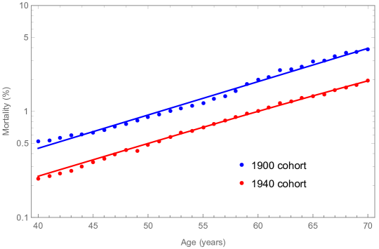
Figure 1: Mortality rates (log scale) at adults’ ages for the cohorts born in 1900 and 1940 in the US. The dots are actual data (Berkeley Human Mortality Database) and the lines are model-implied mortality curves.

At the intuitive level, this “shift down” of mortality across generations can be ascribed to continuous improvement of healthcare and accumulation of wealth. Understanding precisely how this “shift down” materializes demands careful modeling in which wealth evolution, healthcare choices, and the resulting mortality are all endogenous. Standard models of consumption and investment do not seem to serve the purpose: the majority, e.g. [35], [25], [26], and [30], consider no more than exogenous mortality, leaving no room for healthcare.

Recently, Guasoni and Huang [15] directly modeled the effect of healthcare on mortality: healthcare reduces Gompertz’ natural growth rate of mortality, through an efficacy function that characterizes the effect of healthcare spending in a society. Healthcare, as a result, indirectly increases utility from consumption accumulated over a longer lifetime. Under the constant relative risk aversion (CRRA) utility function $U(x)=\frac{x^{1-\gamma}}{1-\gamma}$, $0<\gamma<1$, an optimal strategy of consumption, investment, and healthcare spending is derived in [15], where the constraint $0<\gamma<1$ is justified by interpreting $1/\gamma$ as an agent’s elasticity of intertemporal substitution (EIS). Specifically, to model mortality endogenously, we need to be cautious of potential preference for death over life. To avoid this, [15] assumes that an agent can leave a fraction $\zeta\in(0,1]$, not necessarily all, of his wealth at death to beneficiaries, reflecting the effect of inheritance and estate taxes. It is shown in [15] that the optimization problem is ill-posed for $\gamma>1$. Indeed, with $\gamma>1$, or EIS less than one, the income effect of future loss of wealth at death is so substantial that the agent reduces current consumption to zero, leading to the ill-posedness; see below [15, Proposition 3.2] for details.

Despite the progress in [15], the artificial relation that EIS is the reciprocal of relative risk aversion, forced by CRRA utility functions, significantly restricts its applications. Although a preliminary calibration was carried out in [15, Section 5], it was not based on the full-fledged model in [15], but a simplified version without any risky asset. Indeed, once a risky asset is considered, it is unclear whether $\gamma$ should be calibrated to relative risk aversion or EIS. More crucially, empirical studies largely reject relative risk aversion and EIS being reciprocals to each other: it is widely accepted that EIS is larger than one (see e.g. [3], [2], [6], and [5]), while numerous estimates of relative risk aversion are also larger than one (see e.g. [32], [3], and [17]).

In this paper, we investigate optimal consumption, investment, and healthcare spending under preferences of Epstein-Zin type, which disentangle relative risk aversion (denoted by $0<\gamma\neq 1$) and EIS (denoted by $\psi>0$). In particular, we impose throughout the paper

Assumption 1.

$\psi>1$ and $\gamma>{1}/{\psi}$.

This specification implies a preference for early resolution of uncertainty (as explained in [31]), and conforms to empirical estimations mentioned above.

Our Epstein-Zin utility process has several distinctive features. First, it is defined on a random horizon $\tau$, the death time of an agent. Prior studies on Epstein-Zin utilities focus on a fixed-time horizon; see e.g. [8], [28], [23], [29], [22], and [34]. To the best our knowledge, random-horizon Epstein-Zin utilities are developed for the first time in Aurand and Huang [1], where the horizon is assumed to be a stopping time adapted to the market filtration. Our studies complement [1], by allowing for a stopping time (i.e. the death time) that need not depend on the financial market. Second, the random horizon $\tau$ is controllable: one slows the growth of mortality via healthcare spending, which in turn changes the distribution of $\tau$. Note that a controllable random horizon was considered in a few prior studies, e.g. [21] and [9], but all under time-separable utilities. Third, to formulate our Epstein-Zin utilities, we need not only a given consumption stream $c$ (as in the literature), but also a specified healthcare spending process $h$. Given the pair $(c,h)$, the Epstein-Zin utility is defined as the right-continuous process $\widetilde{V}^{c,h}$ that satisfies a random-horizon dynamics (i.e. (2.6) below), with a jump at time $\tau$. Thanks to techniques of filtration expansion, we decompose $\widetilde{V}^{c,h}$ as a function of $\tau$ and a process $V^{c,h}$ that solves an infinite-horizon backward stochastic differential equation (BSDE) under solely the market filtration; see Proposition 2.1. That is, the randomness from death and from the market can be dealt with separately. By deriving a comparison result for this infinite-horizon BSDE (Proposition 2.2), we are able to uniquely determine the Epstein-Zin utility $\widetilde{V}^{c,h}$ for any $k$-admissible strategy $(c,h)$ (Definition 2.3); see Theorem 2.1.

In a Black-Scholes financial market, we maximize the time-0 Epstein-Zin utility $\widetilde{V}^{c,h}_{0}$ over permissible strategies $(c,\pi,h)$ of consumption, investment, and healthcare spending (Definition 4.2). First, we derive the associated Hamilton-Jacobi-Bellman (HJB) equation, from which a candidate optimal strategy $(c^{*},\pi^{*},h^{*})$ is deduced. Taking advantage of a scaling property of the HJB equation, we reduce it to a nonlinear ordinary differential equation (ODE), for which a unique classical solution exists on strength of the Perron method construction in [15]. This, together with a general verification theorem (Theorem 3.1), yields the optimality of $(c^{*},\pi^{*},h^{*})$; see Theorem 4.1.

Compared with classical Epstein-Zin utility maximization, the additional controlled mortality process $M^{h}$ in our case adds nontrivial complexity. In deriving the comparison result Proposition 2.2, standard Gronwall’s inequality cannot be applied due to the inclusion of $M^{h}$. As shown in Appendix A.2, a transformation of processes, as well as the use of both forward and backward Gronwall’s inequalities, are required to circumvent this issue. On the other hand, in carrying out verification arguments, we need to contain the growth of $M^{h}$ to ensure that the Epstein-Zin utility is well-defined. This is done through a combination of probabilistic arguments and analysis of the aforementioned nonlinear ODE; see Appendix A.4 for details.

Our model is calibrated to mortality data in the US and UK. Under the simplifying assumption that the cohort born in 1900 had no healthcare and the cohort born in 1940 had full access to healthcare, we generate an endogenous mortality curve for the 1940 cohort. Figure 1 shows that the model-implied mortality (red line) closely reproduces actual data in the US (red dots). Our model performs well also for the UK data; see Figure 2. We also compute the optimal healthcare spending across different ages (Figure 3(a)) and calibrate the efficacy of healthcare in these two countries (Figure 3(b)).

The rest of the paper is organized as follows. Section 2 establishes Epstein-Zin utilities over one’s random lifetime, with healthcare spending incorporated. Section 3 introduces the problem of optimal consumption, investment, and healthcare spending under Epstein-Zin preferences, and derives the related HJB equation and a general verification theorem. Section 4 characterizes optimal consumption, investment, and healthcare spending in three different settings of aging and access to healthcare. Section 5 calibrates our model to mortality data in the US and UK. Most proofs are collected in Appendix A.

2 Epstein-Zin Preferences with Healthcare Spending

Let $(\Omega,\mathcal{F},\mathbb{P})$ be a probability space equipped with a filtration $\mathbb{F}=(\mathcal{F}_{t})_{t\geq 0}$ that satisfies the usual conditions. Consider another probability space $(\Omega^{\prime},\mathcal{F}^{\prime},\mathbb{P}^{\prime})$ supporting a random variable $Z$ that has an exponential law

$$\mathbb{P}^{\prime}(Z>z)=e^{-z},\quad z\geq 0.$$ (2.1)

We denote by $(\bar{\Omega},\bar{\mathcal{F}},\bar{\mathbb{P}})$ the product probability space $(\Omega\times\Omega^{\prime},\mathcal{F}\times\mathcal{F}^{\prime},\mathbb{P}\times\mathbb{P}^{\prime})$. The expectations taken under $\mathbb{P}$, $\mathbb{P}^{\prime}$, and $\bar{\mathbb{P}}$ will be denoted by $\mathbb{E}$, $\mathbb{E}^{\prime}$, and $\bar{\mathbb{E}}$, respectively.

Consider an agent who obtains utility from consumption, partially determines his lifespan through healthcare spending, and has bequest motives to leave his wealth at death to beneficiaries. Specifically, we assume that the mortality rate process $M$ of the agent evolves as

$$dM_{t}=(\beta-g(h_{t}))M_{t}dt,\quad M_{0}=m>0,$$ (2.2)

where $h=(h_{t})_{t\geq 0}$, a nonnegative $\mathbb{F}$-progressively measurable process, represents the proportion of wealth spent on healthcare at each time $t$, while $g:\mathbb{R}_{+}\to\mathbb{R}_{+}$ is the efficacy function that prescribes how much the natural growth rate of mortality $\beta>0$ is reduced by healthcare spending $h_{t}$. For any $\bar{\omega}=(\omega,\omega^{\prime})\in\bar{\Omega}$, the random lifetime of the agent is formulated as

$$\tau(\bar{\omega}):=\inf\left\{t\geq 0:\int_{0}^{t}M_{s}^{h}(\omega)ds\geq{Z}(\omega^{\prime})\right\}.$$ (2.3)

The information available to the agent is then defined as $\mathbb{G}=(\mathcal{G}_{t})_{t\geq 0}$ with

$$\mathcal{G}_{t}:=\mathcal{F}_{t}\vee\mathcal{H}_{t},\quad\hbox{where}\quad\mathcal{H}_{t}:=\sigma\left(\mathbbm{1}_{\{\tau\leq u\}},u\in[0,t]\right).$$ (2.4)

That is, at any time $t$, the agent knows the information contained in $\mathcal{F}_{t}$ and whether he is still alive (i.e. whether $\tau>t$ holds); he has no further information of $\tau$, as the random variable $Z$ is inaccessible to him. Finally, we assume that the agent can leave a fraction $\zeta\in(0,1]$, not necessarily all, of his wealth at death to beneficiaries, reflecting the effect of inheritance and estate taxes.

Remark 2.1.

As a modeling simplification mainly for the purpose of tractability, the controlled mortality (2.2) (borrowed from [15]) assumes that healthcare expenses relative to wealth, rather than in absolute terms, affect mortality growth.

Now, let us define a non-standard Epstein-Zin utility process that incorporates healthcare spending. First, recall the Epstein-Zin aggregator $f:\mathbb{R}_{+}\times\mathbb{R}\to\mathbb{R}$ given by

$$\begin{split}f(c,v)&:=\delta\frac{(1-\gamma)v}{1-\frac{1}{\psi}}\left(\bigg{(}\frac{c}{((1-\gamma)v)^{\frac{1}{1-\gamma}}}\bigg{)}^{1-\frac{1}{\psi}}-1\right)\\ &=\delta\frac{c^{1-\frac{1}{\psi}}}{1-\frac{1}{\psi}}\big{(}(1-\gamma)v\big{)}^{1-\frac{1}{\theta}}-\delta\theta v,\qquad\text{with}\quad\theta:=\frac{1-\gamma}{1-\frac{1}{\psi}},\end{split}$$ (2.5)

where $\gamma$ and $\psi$ represent the agent’s relative risk aversion and EIS, respectively, as stated in Section 1. Given a consumption stream $c=(c_{t})_{t\geq 0}$, assumed to be nonnegative $\mathbb{F}$-progressively measurable, and a healthcare spending process $h=(h_{t})_{t\geq 0}$ introduced below (2.2), we define the Epstein-Zin utility on the random horizon $\tau$ to be a $\mathbb{G}$-adapted semimartingale $(\widetilde{V}_{t}^{c,h})_{t\geq 0}$ satisfying

$$\widetilde{V}_{t}^{c,h}=\bar{\mathbb{E}}_{t}\left[\int_{t\wedge\tau}^{T\wedge\tau}f(c_{s},\widetilde{V}_{s}^{c,h})ds+\zeta^{1-\gamma}\widetilde{V}_{\tau-}^{c,h}\mathbbm{1}_{\{\tau\leq T\}}+\widetilde{V}_{T}^{c,h}\mathbbm{1}_{\{\tau>T\}}\right],\text{ for all }0\leq t\leq T<\infty,$$ (2.6)

where we use the notation $\bar{\mathbb{E}}_{t}\left[\cdot\right]=\bar{\mathbb{E}}\left[\cdot|\mathcal{G}_{t}\right]$. In (2.6), we assert that the loss of wealth at death results in a decreased bequest utility, by a factor of $\zeta^{1-\gamma}$. This assertion will be made clear and justified in Section 4, where a financial model is in place; see Remark 4.4 particularly.

Before solving (2.6) for $(\widetilde{V}^{c,h}_{t})_{t\geq 0}$, we introduce a general definition of infinite-horizon BSDEs.

Definition 2.1.

Let $V$ be an $\mathbb{F}$-progressively measurable process satisfying $\mathbb{E}[\sup_{s\in[0,t]}|V_{s}|]<\infty$ for all $t\geq 0$. For any $G:\Omega\times\mathbb{R}_{+}\times\mathbb{R}\to\mathbb{R}$, we say $V$ is a solution to the infinite-horizon BSDE

$$dV_{t}=-G(\omega,t,V_{t})dt+d\mathscr{M}_{t},$$ (2.7)

if the following conditions hold: (i) $\big{(}G(\cdot,t,V_{t}(\cdot))\big{)}_{t\geq 0}$ is $\mathbb{F}$-progressively measurable, and (ii) for any $T>0$ there exists an $\mathbb{F}$-martingale $(\mathscr{M}_{t})_{t\in[0,T]}$ such that (2.7) holds for $0\leq t\leq T$.

Remark 2.2.

Without a terminal condition, (2.7) can have infinitely many solutions. Indeed, as long as $G$ admits proper monotonicity, there are solutions to (2.7) that satisfy “$\lim_{t\to\infty}V_{t}=\xi$ for $\mathcal{F}$-measurable random variable $\xi$” or “$\lim_{t\to\infty}\mathbb{E}\left[e^{\rho t}V_{t}\right]\rightarrow 0$ for $\rho>0$”; see [7] and [12]. We will address this non-uniqueness issue by enforcing appropriate “terminal behavior”; see Remark 2.6.

The next result shows that the $\mathbb{G}$-adapted $\widetilde{V}$ in (2.6) can be expressed as a function of $\tau$ and an $\mathbb{F}$-adapted process $V$ that satisfies an infinite-horizon BSDE.

Proposition 2.1.

Let $c,h$ be nonnegative $\mathbb{F}$-progressively measurable. Then, $\widetilde{V}$ is a $\mathbb{G}$-adapted semimartingale, with $\bar{\mathbb{E}}[\sup_{s\in[0,t]}|\widetilde{V}_{s}|]<\infty$ for all $t\geq 0$, that satisfies (2.6) if and only if

$$\widetilde{V}_{t}=V_{t}\mathbbm{1}_{\{t<\tau\}}+\zeta^{1-\gamma}V_{\tau-}\mathbbm{1}_{\{t\geq\tau\}}\qquad\forall t\geq 0,$$ (2.8)

where $V$ is an $\mathbb{F}$-adapted semimartingale, with $\mathbb{E}[\sup_{s\in[0,t]}|V_{s}|]<\infty$ for all $t\geq 0$, that satisfies the infinite-horizon BSDE

$$dV_{t}=-F(c_{t},M_{t}^{h},V_{t})ds+d\mathscr{M}_{t},$$ (2.9)

with $F:\mathbb{R}_{+}\times\mathbb{R}_{+}\times\mathbb{R}\to\mathbb{R}$ defined by

$$F(c,m,v):=f(c,v)-(1-\zeta^{1-\gamma})mv.$$ (2.10)

Proof.

See Section A.1. ∎

Remark 2.3.

Proposition 2.1 actually holds more generally beyond the specific driver $f$ in (2.5) and the boundary condition “$\widetilde{V}_{T}=\zeta^{1-\gamma}\widetilde{V}_{\tau-}$” for $T\geq\tau$ encoded in (2.6). Specifically, in (2.6), if we allow for a general Borel driver $f$ and replace $\zeta^{1-\gamma}\widetilde{V}_{\tau-}$ therein by $H(\widetilde{V}_{\tau-})$ for a general continuous function $H$ that grows at most linearly, the arguments in the proof of Proposition 2.1 (see Section A.1) still hold, leading to an upgraded version of Proposition 2.1 with $\zeta^{1-\gamma}V_{\tau-}$ in (2.8) and $\zeta^{1-\gamma}v$ in (2.10) replaced by $H(V_{\tau-})$ and $H(v)$, respectively.

In view of Proposition 2.1, to uniquely determine the Epstein-Zin utility process $\widetilde{V}$, we need to find a suitable class of stochastic processes among which there exists a unique solution to (2.9). To this end, we start with imposing appropriate integrability and transversality conditions.

Definition 2.2.

For any $k\in\mathbb{R}$, define $\Lambda:=\delta\theta+(1-\theta)k$. Then, for any nonnegative $\mathbb{F}$-progressively measurable $h$, we denote by $\mathcal{E}^{h}_{k}$ the set of all $\mathbb{F}$-adapted semimartingales $Y$ that satisfy the following integrability and transversality conditions:

$$\mathbb{E}\bigg{[}\sup\limits_{s\in[0,t]}\left|Y_{s}\right|\bigg{]}<\infty\ \ \forall t>0\quad\hbox{and}\quad\lim\limits_{t\rightarrow\infty}e^{-\Lambda t}\mathbb{E}\left[e^{-\gamma(\psi-1)\frac{1-\zeta^{1-\gamma}}{1-\gamma}\int_{0}^{t}M_{s}^{h}ds}|Y_{t}|\right]=0.$$ (2.11)

Remark 2.4.

Condition (2.11) is similar to [24, (2.3)], but the controlled mortality $M^{h}$ in our case complicates the transversality condition: unlike [24, (2.3)], the exponential term no longer contains a constant rate, but a stochastic one involving $M^{h}$. This adds nontrivial complexity to deriving a comparison result (Proposition 2.2) and the use of verification arguments (Theorem 4.1).

Remark 2.5.

The constant $\Lambda:=\delta\theta+(1-\theta)k$ in (2.11) can be negative, even when $k>0$ (as will be assumed in Section 4). In such a case, (2.11) stipulates that $M^{h}$ must increase fast enough to neutralize the growth of $e^{-\Lambda t}$, such that the transversality condition can be satisfied.

We now introduce the appropriate collection of strategies $(c,h)$ we will focus on.

Definition 2.3.

Let $c,h$ be nonnegative $\mathbb{F}$-progressively measurable. For any $k\in\mathbb{R}$, we say $(c,h)$ is $k$-admissible if there exists $V\in\mathcal{E}^{h}_{k}$ satisfying (2.9) and

$$V_{s}\leq\delta^{\theta}\left(k+(\psi-1)\frac{1-\zeta^{1-\gamma}}{1-\gamma}M^{h}_{s}\right)^{-\theta}\frac{c_{s}^{1-\gamma}}{1-\gamma},\quad\forall s\geq 0.$$ (2.12)

Remark 2.6.

Condition (2.12) is the key to a comparison result for (2.9), as shown in Proposition 2.2 below. In a sense, (2.11)-(2.12) is the enforced “terminal behavior”, under which a solution to (2.7) can be uniquely identified. Technically, (2.12) is similar to typical conditions imposed for infinite-horizon BSDEs, such as [7, (H1’)] and the one in [12, Theorem 5.1]: all of them require the solution to be bounded from above by a tractable process. Moreover, for classical Epstein-Zin utilities (without healthcare), a similar condition was imposed in [24, (2.5)]. In fact, Definition 2.3 is in line with [24, Definition 2.1], but adapted to include the controlled mortality $M^{h}$.

A comparison result for BSDE (2.9) can now be established.

Proposition 2.2.

Let $k\in\mathbb{R}$ and $c,h$ be nonnegative $\mathbb{F}$-progressively measurable processes. Suppose that $V^{1}\in\mathcal{E}_{k}^{h}$ is a solution to (2.9) and $V^{2}\in\mathcal{E}_{k}^{h}$ is a solution to (2.7). If $V^{1}$ satisfies (2.12) and $F(c_{t},M_{t},V_{t}^{2})\leq G(t,V_{t}^{2})\ d\mathbb{P}\times dt$-a.e., then $V_{t}^{1}\leq V_{t}^{2}$ for $t\geq 0$ $\mathbb{P}$-a.s.

Proof.

See Section A.2. ∎

The next result is a direct consequence of Propositions 2.1 and 2.2.

Theorem 2.1.

Fix $k\in\mathbb{R}$. For any $k$-adimissible $(c,h)$, there exists a unique solution $V^{c,h}\in\mathcal{E}^{h}_{k}$ to (2.9) that satisfies (2.12). Hence, the Epstein-Zin utility $\widetilde{V}^{c,h}$ can be uniquely determined via (2.8).

Remark 2.7.

Results in this section in fact hold true more generally, for certain specifications of $(\psi,\gamma)$ that do not fulfill Assumption 1. For instance, for the cases “$\psi\in(0,1)$, $\gamma>\frac{1}{\psi}$” and “$\psi,\gamma\in(0,1)$”, Theorem 2.1 can be similarly established by suitably adjusting (2.11)-(2.12). This will allow the main result of this paper, Theorem 4.1 below, to be generalized to these cases.

3 Problem Formulation

Let $B=(B_{t})_{t\geq 0}$ be an $\mathbb{F}$-adapted standard Brownian motion. Consider a financial market with a riskfree rate $r>0$ and a risky asset $S_{t}$ given by

$$dS_{t} =(\mu+r)S_{t}dt+\sigma S_{t}dB_{t},$$ (3.1)

where $\mu\in\mathbb{R}$ and $\sigma>0$ are given constants. Given initial wealth $x>0$, at each time $t\geq 0$, an agent chooses a consumption rate $c_{t}$, invests a fraction $\pi_{t}$ of his wealth on the risky asset, and spends another fraction $h_{t}$ on healthcare. The resulting dynamics of the wealth process $X$ is

$$dX_{t} =X_{t}\left(r+\mu\pi_{t}-h_{t}\right)dt-c_{t}dt+X_{t}\sigma\pi_{t}dB_{t},\quad X_{0}=x.$$ (3.2)

Definition 3.1.

For all $k\in\mathbb{R}$, let $\mathcal{H}_{k}$ be the set of strategies $(c,\pi,h)$ such that $(c,h)$ is $k$-admissible (Definition 2.3), $\pi$ is $\mathbb{F}$-progressively measurable, and a unique solution $X^{c,\pi,h}$ to (3.2) exists.

The agent aims at maximizing his lifetime Epstein-Zin utility $\widetilde{V}_{0}^{c,h}$ by choosing $(c,\pi,h)$ in a suitable collection of strategies $\mathcal{P}$, i.e.

$$\sup\limits_{(c,\pi,h)\in\mathcal{P}}\widetilde{V}_{0}^{c,h} =\sup\limits_{(c,\pi,h)\in\mathcal{P}}V_{0}^{c,h},$$ (3.3)

where the equality follows from (2.8). In this section, we only require $\mathcal{P}$ to satisfy

$$\mathcal{P}\subseteq\mathcal{H}_{k}\quad\hbox{for some}\ k\in\mathbb{R}.$$ (3.4)

Our focus is to establish a versatile verification theorem under merely (3.4). A more precise definition of $\mathcal{P}$, depending on specification of $\beta$, $\gamma$, and $\zeta$, will be introduced in Definition 4.2.

3.1 A General Verification Theorem

Under the current Markovian setting (i.e. (3.1) and (3.2)), we take

$$v(x,m):=\sup\limits_{(c,\pi,h)\in\mathcal{P}}V_{0}^{c,h},$$ (3.5)

i.e. the optimal value should be a function of the current wealth and mortality. The relation (A.10), derived from (2.6), suggests the following dynamic programming principle: With the shorthand notation $\mathfrak{p}=(c,\pi,h)$ and $\mathfrak{p}_{s}=(c_{s},\pi_{s},h_{s})$ for $s\geq 0$, for any $T>0$,

$$v(x,m)=$$

$$\sup\limits_{\mathfrak{p}\in\mathcal{P}}\mathbb{E}\left[\int_{0}^{T}e^{-\int_{0}^{s}M_{r}^{h}dr}\left(f(c_{s},v(X_{s}^{\mathfrak{p}},M_{s}^{h}))+\zeta^{1-\gamma}M_{s}^{h}v(X_{s}^{\mathfrak{p}},M_{s}^{h})\right)ds+e^{-\int_{0}^{T}M_{s}ds}v(X_{T}^{\mathfrak{p}},M_{T}^{h})\right].$$ (3.6)

By applying Itô’s formula to $e^{-\int_{0}^{t}M_{s}^{h}ds}v(X_{t}^{\mathfrak{p}},M_{t}^{h})$, assuming enough regularity of $v$, we get

$$e^{-\int_{0}^{T}M_{s}^{h}ds}v(X_{T}^{\mathfrak{p}},M_{T}^{h})-v(x,m)$$

$$=\int_{0}^{T}\left(L^{\mathfrak{p}_{s}}[v](X_{t}^{\mathfrak{p}},M_{t}^{h})-M_{t}^{h}v(X_{t}^{\mathfrak{p}},M_{t}^{h})\right)dt+\int_{0}^{T}e^{-\int_{0}^{t}M_{s}^{h}ds}\sigma\pi X_{t}^{\mathfrak{p}}v_{x}(X_{t}^{\mathfrak{p}},M_{t}^{h})dB_{t},$$

where the operator $L^{a,b,d}[\cdot]$ is defined by

$$L^{a,b,d}[\kappa](x,m):=\left((r+\mu b-d)x-a\right)\kappa_{x}(x,m)+(\beta-g(d))m\kappa_{m}(x,m)+\frac{1}{2}\sigma^{2}b^{2}x^{2}\kappa_{xx}(x,m),$$ (3.7)

for any $\kappa\in C^{2,1}(\mathbb{R}_{+}\times\mathbb{R}_{+})$. We can then rewrite (3.1) as

$$0=\sup\limits_{\mathfrak{p}\in\mathcal{P}}\mathbb{E}\left[\int_{0}^{T}e^{-\int_{0}^{s}M_{t}^{h}dt}\left(f(c_{s},v(X_{s}^{\mathfrak{p}},M_{s}^{h}))+(\zeta^{1-\gamma}-1)M_{s}^{h}v(X_{s}^{\mathfrak{p}},M_{s}^{h})+L^{\mathfrak{p}_{s}}[v](X_{s}^{\mathfrak{p}},M_{s}^{h})\right)ds\right].$$

The HJB equation associated with $v(x,m)$ is then

$$0 =\sup\limits_{c\in\mathbb{R}_{+}}\left\{f(c,w(x,m))-cw_{x}(x,m)\right\}+\sup\limits_{h\in\mathbb{R}_{+}}\left\{-g(h)mw_{m}(x,m)-hxw_{x}(x,m)\right\}$$

$$\hskip 14.45377pt+\sup\limits_{\pi\in\mathbb{R}}\left\{\mu\pi xw_{x}(x,m)+\frac{1}{2}\sigma^{2}\pi^{2}x^{2}w_{xx}(x,m)\right\}$$ (3.8)

$$\hskip 14.45377pt+rxw_{x}(x,m)+\beta mw_{m}(x,m)+(\zeta^{1-\gamma}-1)mw(x,m),\quad\forall(x,m)\in\mathbb{R}_{+}^{2}.$$

Equivalently, this can be written in the more compact form

$$\sup\limits_{c,h\in\mathbb{R}_{+},\pi\in\mathbb{R}}\left\{L^{c,\pi,h}[w](x,m)+f(c,w(x,m))\right\}+(\zeta^{1-\gamma}-1)mw(x,m)=0,\quad\forall(x,m)\in\mathbb{R}_{+}^{2}.$$ (3.9)

Theorem 3.1.

Let $w\in C^{2,1}(\mathbb{R}_{+}\times\mathbb{R}_{+})$ be a solution to (3.1) and $\mathcal{P}$ satisfy (3.4). Suppose for any $(c,\pi,h)\in\mathcal{P}$, the process $w(X_{t}^{c,\pi,h},M_{t}^{h})$, $t\geq 0$, belongs to $\mathcal{E}^{h}_{k}$ (with $k\in\mathbb{R}$ specified by (3.4)) and

$$\mathbb{E}\bigg{[}\sup_{s\in[0,t]}\pi_{s}X^{c,\pi,h}_{s}w_{x}(X_{s}^{c,\pi,h},M_{s}^{h})\bigg{]}<\infty,\quad\forall t>0.$$ (3.10)

Then, the following holds.

• $w(x,m)\geq v(x,m)$ on $\mathbb{R}_{+}\times\mathbb{R}_{+}$.

• Suppose further that there exist Borel measurable functions $\bar{c},\bar{\pi},\bar{h}:\mathbb{R}^{2}_{+}\to\mathbb{R}$ such that $\bar{c}(x,m)$, $\bar{\pi}(x,m)$, and $\bar{h}(x,m)$ are maximizers of

  $$\sup\limits_{c\in\mathbb{R}_{+}}\left\{f(c,w(x,m))-cw_{x}(x,m)\right\},\quad\sup\limits_{\pi\in\mathbb{R}}\left\{\mu\pi xw_{x}(x,m)+\frac{1}{2}\sigma^{2}\pi^{2}x^{2}w_{xx}(x,m)\right\},$$ (3.11)

  $$\hskip 86.72377pt\sup\limits_{h\in\mathbb{R}_{+}}\left\{-g(h)mw_{m}(x,m)-hxw_{x}(x,m)\right\},$$ (3.12)

  respectively, for all $(x,m)\in\mathbb{R}^{2}_{+}$. If $(c^{*},\pi^{*},h^{*})$ defined by

  $$c^{*}_{t}:=\bar{c}(X_{t},M_{t}),\quad\pi^{*}_{t}:=\bar{\pi}(X_{t},M_{t}),\quad h^{*}_{t}:=\bar{h}(X_{t},M_{t}),\qquad t\geq 0,$$ (3.13)

  belongs to $\mathcal{P}$ and $W^{*}_{t}:=w(X_{t}^{c^{*},\pi^{*},h^{*}},M_{t}^{h^{*}})$ satisfies (2.12) (with $V$, $c$, $h$ replaced by $W^{*}$, $c^{*}$, $h^{*}$), then $(c^{*},\pi^{*},h^{*})$ optimizes (3.5) and $w(x,m)=v(x,m)$ on $\mathbb{R}_{+}\times\mathbb{R}_{+}$.

Proof.

(i) Fix $(x,m)\in\mathbb{R}^{2}_{+}$. Consider an arbitrary $\mathfrak{p}=(c,\pi,h)\in\mathcal{P}$. For any $T\geq 0$ and $t\in[0,T]$, by applying Itô’s formula to $w(X^{\mathfrak{p}}_{s},M^{h}_{s})$, we get

$$w(X_{T}^{\mathfrak{p}},M_{T}^{h})=w(X_{t}^{\mathfrak{p}},M_{t}^{h})+\int_{t}^{T}L^{\mathfrak{p}_{s}}[w](X_{s}^{\mathfrak{p}},M_{s}^{h})ds+\int_{t}^{T}\sigma\pi_{s}X_{s}^{\mathfrak{p}}w_{x}(X_{s}^{\mathfrak{p}},M_{s}^{h})dB_{s},$$

where the operator $L^{a,b,d}[\cdot]$ is defined in (3.7). Thanks to (3.10), $u\mapsto\int_{t}^{u}\sigma\pi_{s}X_{s}^{\mathfrak{p}}w_{x}(X_{s}^{\mathfrak{p}},M_{s}^{h})dB_{s}$ is a true martingale. Hence, the above equality shows that $W_{s}:=w(X_{s}^{\mathfrak{p}},M_{s}^{h})$ is a solution to BSDE (2.7), with $G(\omega,s,v):=-L^{\mathfrak{p}_{s}(\omega)}[w](X_{s}^{\mathfrak{p}}(\omega),M_{s}^{h}(\omega))$. On the other hand, (3.4) implies that $(c,h)$ is $k$-admissible, so that there exists a unique solution $V^{c,h}\in\mathcal{E}^{h}_{k}$ to (2.9) that satisfies (2.12) (Theorem 2.1). Since $w$ is a solution to (3.1), and equivalently to (3.9), we have

$$F(c_{s},M^{h}_{s},W_{s})=f(c_{s},W_{s})+(\zeta^{1-\gamma}-1)M_{s}^{h}W_{s}\leq-L^{\mathfrak{p}_{s}}[w](X_{s}^{\mathfrak{p}},M_{s}^{h}).$$ (3.14)

We then conclude from Proposition 2.2 that $W_{t}\geq V_{t}^{c,h}$ for all $t\geq 0$. In particular, $w(x,m)=W_{0}\geq V_{0}^{c,h}$. By the arbitrariness of $(c,\pi,h)\in\mathcal{P}$, $w(x,m)\geq\sup_{(c,\pi,h)\in\mathcal{P}}V_{0}^{c,h}=v(x,m)$, as desired.

(ii) Fix $(x,m)\in\mathbb{R}^{2}_{+}$. If $(c^{*},\pi^{*},h^{*})\in\mathcal{P}$, we can repeat the arguments in part (a), obtaining (3.14) with the inequality replaced by equality. This shows that $W^{*}_{t}=w(X^{c^{*},\pi^{*},h^{*}}_{t},M^{h^{*}}_{t})\in\mathcal{E}^{h^{*}}_{k}$ is a solution to (2.9). Also, (3.4) implies that $(c^{*},h^{*})$ is $k$-admissible, so that there is a unique solution $V^{c^{*},h^{*}}\in\mathcal{E}^{h^{*}}_{k}$ to (2.9) satisfying (2.12) (Theorem 2.1). As $W^{*}$ also satisfies (2.12), we have $W^{*}_{t}=V^{c^{*},h^{*}}_{t}$ for all $t\geq 0$; particularly, $w(x,m)=W^{*}_{0}=V^{c^{*},h^{*}}_{0}$. With $w(x,m)\geq\sup_{(c,\pi,h)\in\mathcal{P}}V_{0}^{c,h}=v(x,m)$ in part (a), we conclude $w(x,m)=v(x,m)$ and $(c^{*},\pi^{*},h^{*})\in\mathcal{P}$ is an optimal control. ∎

3.2 Reduction to an Ordinary Differential Equation

If we assume heuristically that $w_{xx}<0$, $w_{m}<0$, $g$ is differentiable, and the inverse of $g^{\prime}$ is well-defined, then the optimizers stated in Theorem 3.1 (ii) can be uniquely determined as

$$\begin{split}\bar{c}(x,m)&=\delta^{\psi}\frac{\left[(1-\gamma)w(x,m)\right]^{\psi(1-\frac{1}{\theta})}}{w_{x}(x,m)^{\psi}},\quad\bar{\pi}(x,m)=-\frac{\mu}{\sigma^{2}}\frac{w_{x}(x,m)}{xw_{xx}(x,m)},\\ &\hskip 36.135pt\bar{h}(x,m)=(g^{\prime})^{-1}\left(-\frac{xw_{x}(x,m)}{mw_{m}(x,m)}\right).\end{split}$$ (3.15)

Plugging these into (3.1) yields

$$0 =\frac{\delta^{\psi}}{\psi-1}\frac{\left[(1-\gamma)v(x,m)\right]^{\psi(1-\frac{1}{\theta})}}{v_{x}(x,m)^{\psi-1}}-\delta\theta v(x,m)-\frac{1}{2}\left(\frac{\mu}{\sigma}\right)^{2}\frac{v_{x}(x,m)^{2}}{v_{xx}(x,m)}+rxv_{x}(x,m)+\beta mv_{m}(x,m)$$

$$\hskip 14.45377pt+(\zeta^{1-\gamma}-1)mv(x,m)-mv_{m}(x,m)\sup\limits_{h\in\mathbb{R}_{+}}\left\{g(h)+\frac{hxv_{x}(x,m)}{mv_{m}(x,m)}\right\}.$$ (3.16)

Using the ansatz $w(x,m)=\delta^{\theta}\frac{x^{1-\gamma}}{1-\gamma}u(m)^{-\frac{\theta}{\psi}}$, the above equation reduces to

$$0 =u(m)^{2}-\tilde{c}_{0}(m)u(m)-\beta mu^{\prime}(m)+mu^{\prime}(m)\sup\limits_{h\in\mathbb{R}_{+}}\left\{g(h)-(\psi-1)\frac{u(m)}{mu^{\prime}(m)}h\right\},\quad m>0,$$ (3.17)

where

$$\tilde{c}_{0}(m) :=\psi\delta+(1-\psi)\bigg{(}\frac{(\zeta^{1-\gamma}-1)m}{1-\gamma}+r+\frac{1}{2\gamma}\left(\frac{\mu}{\sigma}\right)^{2}\bigg{)}.$$ (3.18)

Moreover, the maximizers in (3.15) now become

$$\bar{c}(x,m)=xu(m),\quad\bar{\pi}\equiv\frac{\mu}{\gamma\sigma^{2}},\quad\bar{h}(m)=(g^{\prime})^{-1}\left((\psi-1)\frac{u(m)}{mu^{\prime}(m)}\right).$$ (3.19)

These maximizers indeed characterize optimal consumption, investment, and healthcare spending, as will be shown in the next section.

4 The Main Results

Let us now formulate the set $\mathcal{P}$ of permissible strategies $(c,\pi,h)$ in the optimization problem (3.3). First, take $k\in\mathbb{R}$ in Definition 2.2 to be

$$k^{*}:=\delta\psi+(1-\psi)\bigg{(}r+\frac{1}{2\gamma}\left(\frac{\mu}{\sigma}\right)^{2}\bigg{)},$$ (4.1)

so that $\Lambda\in\mathbb{R}$ in Definition 2.2 becomes

$$\Lambda^{*}:=\delta\theta+(1-\theta)k^{*}=\delta\gamma\psi+(1-\gamma\psi)\left(r+\frac{1}{2\gamma}\left(\frac{\mu}{\sigma}\right)^{2}\right).$$ (4.2)

Definition 4.1.

Let $\mathcal{P}_{1}$ the set of strategies $(c,\pi,h)$ such that $(c,\pi,h)\in\mathcal{H}_{k^{*}}$, $(X^{c,\pi,h})^{1-\gamma}$ satisfies (2.11) (with $\Lambda\in\mathbb{R}$ therein taken to be $\Lambda^{*}$) as well as $\mathbb{E}\big{[}\sup_{s\in[0,t]}\pi_{s}(X^{c,\pi,h}_{s})^{1-\gamma}\big{]}<\infty$ for $t\geq 0.$

Let $\mathcal{P}_{2}$ be defined as $\mathcal{P}_{1}$, except that the second part of (2.11) is replaced by

$$\lim_{t\rightarrow\infty}e^{-\Lambda^{*}t}\mathbb{E}\left[e^{-\eta\gamma(\psi-1)\frac{1-\zeta^{1-\gamma}}{1-\gamma}\int_{0}^{t}M_{s}^{h}ds}(X_{t}^{c,\pi,h})^{1-\gamma}\right]=0,\quad\hbox{for some $\eta\in(1-\frac{1}{\gamma},1)$}.$$ (4.3)

Definition 4.2.

The set of permissible strategies $(c,\pi,h)$, denoted by $\mathcal{P}$, is defined as follows.

• For the case $\beta=0$ and $g\equiv 0$ (i.e. with neither aging nor healthcare), $\mathcal{P}:=\mathcal{P}_{1}$;

• For the case $\beta>0$ (i.e. with aging),

  $$\mathcal{P}:=\begin{cases}\mathcal{P}_{1},\quad&\hbox{if}\ \gamma\in\big{(}\frac{1}{\psi},1\big{)}\ \hbox{or}\ \zeta=1,\\ \mathcal{P}_{2},\quad&\hbox{if}\ \gamma>1\ \hbox{and}\ \zeta\in(0,1),\end{cases}$$

Remark 4.1.

When there is aging ($\beta>0$), for the case $\gamma>1$ and $\zeta\in(0,1)$, we need $(X^{c,\pi,h})^{1-\gamma}$ to satisfy the slightly stronger condition (4.3) (than the transversality condition in (2.11)), so that the general verification Theorem 3.1 can be applied; see Appendix A.4 for details.

The rest of the section presents main results in three different settings of aging and access to healthcare, in order of complexity.

4.1 Neither Aging nor Healthcare

When the natural growth rate of mortality is zero ($\beta=0$) and healthcare is unavailable ($g\equiv 0$), the mortality process is constant, i.e. $M_{t}\equiv m$. Consequently, in the HJB equation (3.1), all derivatives in $m$ should vanish; also, as $v(x,m)$ is nondecreasing in $x$ by definition, the second supremum in (3.1) should be zero. Corresponding to this largely simplified HJB equation, (3.17) reduces to

$$0=u(m)^{2}-\tilde{c}_{0}(m)u(m),$$

which directly implies $u(m)=\tilde{c}_{0}(m)$. The problem (3.5) can then be solved explicitly.

Proposition 4.1.

Assume $\beta=0$ and $g\equiv 0$. For any $m\geq 0$, if $\tilde{c}_{0}(m)>0$ in (3.18), then

$$v(x,m)=\delta^{\theta}\frac{x^{1-\gamma}}{1-\gamma}\tilde{c}_{0}(m)^{-\frac{\theta}{\psi}}\quad\hbox{for $x>0$.}$$

Furthermore, $c_{t}^{*}:=\tilde{c}_{0}(m)X_{t}$, $\pi^{*}_{t}:=\frac{\mu}{\gamma\sigma^{2}}$, and $h^{*}_{t}:=0$, for $t\geq 0$, form an optimal control for (3.5).

Proof.

See Section A.3. ∎

Proposition 4.1 shows that without aging and healthcare, optimal investment follows classical Merton’s proportion, while the optimal consumption rate is the constant $\tilde{c}_{0}(m)$, dictated by the fixed mortality $m$. By (3.18), for the case $\zeta=1$, $\tilde{c}_{0}(m)\equiv\psi\delta+(1-\psi)\big{(}r+\frac{1}{2\gamma}\left(\frac{\mu}{\sigma}\right)^{2}\big{)}$ no longer depends on $m$. Indeed, with no loss of wealth (and thus utility) at death, dying sooner or later does not make a difference to one who maximizes lifetime utility plus bequest utility.

As $\frac{\zeta^{1-\gamma}-1}{1-\gamma}<0$ for $\zeta<1$ and $0<\gamma\neq 1$, we observe from (3.18) that a larger mortality rate $m$ induces a larger consumption rate due to EIS $\psi>1$. This can be explained by the usual income and substitution effects in response to negative wealth shocks. A larger mortality rate makes the loss of wealth at death more pressing and imminent. This reduces the total income generated by saving up to the death time, leading to the income effect that reduces consumption in the current period. On the other hand, as saving is now less effective in generating future income, the opportunity cost of consumption in the current period decreases. This brings about the substitution effect that increases current consumption. As is known in the literature, when EIS $\psi>1$, the substitution effect prevails, encouraging the agent to consume more.

4.2 Aging without Healthcare

When the natural growth of mortality is positive ($\beta>0$) but healthcare is unavailable ($g\equiv 0$), mortality grows exponentially, i.e. $M_{t}=me^{\beta t}$. As $g\equiv 0$ and $v(x,m)$ is nondecreasing in $x$ by definition, the second supremum in (3.1) vanishes. It follows that (3.17) reduces to

$$0=u(m)^{2}-\tilde{c}_{0}(m)u(m)-\beta mu^{\prime}(m),\quad m>0.$$ (4.4)

This type of differential equations can be solved explicitly.

Lemma 4.1.

Fix $\ell>0$, and define the function $u_{\ell}:\mathbb{R}_{+}\to\mathbb{R}_{+}$ by

$$u_{\ell}(m):=\left(\frac{1}{\ell}\int_{0}^{\infty}e^{\frac{\psi-1}{\ell(1-\gamma)}(\zeta^{1-\gamma}-1)my}(y+1)^{-\left(1+\frac{k^{*}}{\ell}\right)}dy\right)^{-1}.$$ (4.5)

If $k^{*}>0$ in (4.1), then $u_{\ell}$ is the unique solution to the ordinary differential equation

$$0=u^{2}(m)-\tilde{c}_{0}(m)u(m)-\ell mu^{\prime}(m),\quad\forall m>0,$$ (4.6)

such that $\lim_{\ell\rightarrow 0}u_{\ell}(m)=\tilde{c}_{0}(m)$. Moreover, $u_{\ell}$ satisfies

$$u_{\ell}(0)=\tilde{c}_{0}(0)=k^{*}>0,\quad\lim_{m\rightarrow\infty}\left[u_{\ell}(m)-(\tilde{c}_{0}(m)+\ell)\right]=0,$$

$$\tilde{c}_{0}(m)<u_{\ell}(m)<\tilde{c}_{0}(m)+\ell,\quad\forall m>0.$$ (4.7)

Proof.

Similarly to (A.8) in [15], (4.6) admits the general solution

$$u(m)=\ell e^{\frac{\psi}{\theta\ell}(\zeta^{1-\gamma}-1)m}\left(C\beta m^{\frac{k}{\beta}}+\int_{1}^{\infty}e^{\frac{\psi}{\theta\ell}(\zeta^{1-\gamma}-1)mv}v^{-(1+\frac{k}{\ell})}dv\right)^{-1},\quad\hbox{with}\ C\in\mathbb{R}.$$

To ensure $\lim_{\ell\rightarrow 0}u(m)=\tilde{c}_{0}(m)$, we need $C=0$, which identifies the corresponding solution as

$$u_{\ell}(m) =\ell e^{\frac{\psi}{\theta\ell}(\zeta^{1-\gamma}-1)m}\left(\int_{1}^{\infty}e^{\frac{\psi}{\theta\ell}(\zeta^{1-\gamma}-1)mv}v^{-(1+\frac{k}{\ell})}dv\right)^{-1}.$$

A straightforward change of variable then gives the formula (4.5). Now, replacing the positive constants $\frac{\delta+(\gamma-1)r}{\gamma}$, $\beta$, and $\frac{1-\zeta^{1-\gamma}}{\gamma}$ in [15, Lemma A.1] by $k^{*}$, $\ell$, and $-\frac{\psi-1}{1-\gamma}(\zeta^{1-\gamma}-1)$ in our setting, we immediately obtain the remaining assertions. ∎

Proposition 4.2.

Assume $\beta>0$ and $g\equiv 0$. If $k^{*}>0$ in (4.1), then

$$v(x,m)=\delta^{\theta}\frac{x^{1-\gamma}}{1-\gamma}u_{\beta}(m)^{-\frac{\theta}{\psi}},\qquad(x,m)\in\mathbb{R}_{+}^{2},$$

where $u_{\beta}:\mathbb{R}_{+}\to\mathbb{R}_{+}$ is defined as in (4.5), with $\ell=\beta$. Furthermore, $c^{*}_{t}:=u_{\beta}(me^{\beta t})X_{t}$, $\pi^{*}_{t}:=\frac{\mu}{\gamma\sigma^{2}}$, and $h^{*}_{t}:=0$, for $t\geq 0$, form an optimal control for (3.5).

Proof.

See Section A.5. ∎

Observe from (3.18) and (4.1) that

$$\tilde{c}_{0}(m)=k^{*}+(\psi-1)\frac{(1-\zeta^{1-\gamma})m}{1-\gamma}.$$ (4.8)

As $\psi>1$ and $\frac{1-\zeta^{1-\gamma}}{1-\gamma}>0$ for all $0<\gamma\neq 1$, the condition $k^{*}>0$ ensures $\tilde{c}_{0}(m)>0$ for all $m>0$. This, together with $u_{\beta}>\tilde{c}_{0}$ ((4.7) with $\ell=\beta$), shows that $k^{*}>0$ in Proposition 4.2 is essentially a well-posedness condition, ensuring that the optimal consumption rate $u_{\beta}(me^{\beta t})$ is strictly positive for all $t\geq 0$. Moreover, with $\ell=\beta$, (4.7) stipulates that aging enlarges consumption rate, but the increase does not exceed the growth of aging $\beta>0$; note that the increase in consumption results from the same substitution effect as discussed below Proposition 4.1.

4.3 Aging and Healthcare

For the general case where the natural growth of mortality is positive ($\beta>0$) and healthcare is available ($g\not\equiv 0$), we need to deal with the equation (3.17) in its full complexity.

Assumption 2.

Let $g:\mathbb{R}_{+}\to\mathbb{R}_{+}$ be twice differentiable with $g(0)=0$, $g^{\prime}(h)>0$ and $g^{\prime\prime}(h)<0$ for $h>0$, and satisfies the Inada condition

$$g^{\prime}(0+)=\infty\quad\text{and}\quad g^{\prime}(\infty)=0,$$ (4.9)

as well as

$$g\left(I\left(\psi-1\right)\right)<\beta\quad\text{with}\quad I:=(g^{\prime})^{-1}.$$ (4.10)

Condition (4.10) was first introduced in [15]. Its purpose will be made clear after the optimal healthcare spending strategy $h^{*}$ is introduced in Theorem 4.1; see Remark 4.3.

Lemma 4.2.

Suppose Assumption 2 holds. If $k^{*}>0$ in (4.1), there exists a unique nonnegative, strictly increasing, strictly concave, classical solution $u^{*}:\mathbb{R}_{+}\to\mathbb{R}_{+}$ to (3.17). Furthermore, define

$$\underline{\beta}:=\beta-\sup\limits_{h\geq 0}\left\{g(h)-(\psi-1)h\right\}\in(0,\beta).$$

Then, $\lim_{m\rightarrow\infty}\left[u^{*}(m)-(\tilde{c}_{0}(m)+\underline{\beta})\right]=0$ and

$$u_{\underline{\beta}}(m)\leq u^{*}(m)\leq\min\{u_{\beta}(m),\tilde{c}_{0}(m)+\underline{\beta}\}\quad\forall m>0.$$ (4.11)

Proof.

By replacing positive constants $\frac{1-\gamma}{\gamma}$, $\frac{\delta+(1-\gamma)r}{\gamma}$, and $\frac{1-\zeta^{1-\gamma}}{\gamma}$ in [15, Appendix A.3] (particularly Theorems 3.1 and 3.2) by $\psi-1$, $k^{*}$, and $-\frac{\psi-1}{1-\gamma}(\zeta^{1-\gamma}-1)$ in our setting, we get the desired results. ∎

Remark 4.2.

The tractable lower and upper bounds for $u^{*}$ in (4.11) will play a crucial role in verification arguments in the proof of Theorem 4.1 below, as well as calibration in Section 5.

Theorem 4.1.

Suppose Assumption 2 holds. If $k^{*}>0$ in (4.1), then

$$v(x,m)=\delta^{\theta}\frac{x^{1-\gamma}}{1-\gamma}u^{*}(m)^{-\frac{\theta}{\psi}},\quad(x,m)\in\mathbb{R}^{2}_{+},$$ (4.12)

where $u^{*}:\mathbb{R}_{+}\to\mathbb{R}_{+}$ is the unique nonnegative, strictly increasing, strictly concave, classical solution to (3.17). Furthermore, $(c^{*},\pi^{*},h^{*})$ defined by

$$c^{*}_{t}:=u^{*}(M_{t})X_{t},\quad\pi_{t}^{*}:=\frac{\mu}{\gamma\sigma^{2}},\quad h^{*}_{t}:=(g^{\prime})^{-1}\left((\psi-1)\frac{u^{*}(M_{t})}{M_{t}(u^{*})^{\prime}(M_{t})}\right),\qquad t\geq 0$$

is an optimal control for (3.5).

Proof.

See Section A.4. ∎

Theorem 4.1 identifies the marginal efficacy of optimal healthcare spending, $g^{\prime}(h^{*}_{t})$, to be inversely proportional to $\frac{m(u^{*})^{\prime}(m)}{u^{*}(m)}$, the elasticity of consumption with respect to mortality, where the constant of proportionality depends on EIS $\psi$. Note that a larger EIS implies less healthcare spending, as $(g^{\prime})^{-1}$ is strictly decreasing. In a sense, healthcare spending is like saving: it crowds out current consumption, but potentially enlarges future consumption by extending one’s lifetime. Since a larger EIS means a stronger substitution effect (as discussed below Proposition 4.1), one substitutes more consumption for saving-like healthcare spending with a larger $\psi$.

Remark 4.3.

As the same argument in [15, Lemma A.2] implies $\frac{u^{*}(m)}{m(u^{*}(m))^{\prime}}\geq 1$ for $m>0$,

$$g(h^{*}_{t})=g\left(I\left((\psi-1)\frac{u^{*}(M_{t})}{M_{t}(u^{*})^{\prime}(M_{t})}\right)\right)\leq g(I(\psi-1))<\beta,$$ (4.13)

where the last inequality is due to (4.10). In other words, (4.10) stipulates that optimizing healthcare spending can only reduce, but not reverse, the growth of mortality.

Remark 4.4.

Since the transferred wealth at death is $\zeta X^{c^{*},\pi^{*},h^{*}}_{\tau-}$, (4.12) indicates that

$$\delta^{\theta}\frac{(\zeta X^{c^{*},\pi^{*},h^{*}}_{\tau-})^{1-\gamma}}{1-\gamma}u^{*}(M^{h^{*}}_{\tau-})^{-\frac{\theta}{\psi}}=\zeta^{1-\gamma}v(X^{c^{*},\pi^{*},h^{*}}_{\tau-},M^{h^{*}}_{\tau-}),$$

i.e. the loss of wealth at death reduces utility by a factor of $\zeta^{1-\gamma}$, confirming the setup in (2.6).

Remark 4.5.

For the case $\psi=1/\gamma>1$, Propositions 4.1, 4.2 and Theorem 4.1 reduce to results in [15] under time-separable utilities; see Propositions 3.1, 3.2, and Theorems 3.4, 4.1 therein.

5 Calibration: A Preliminary View

In this section, we calibrate the model in Section 4.3 to actual mortality data. We take as given $r=1\%$, $\delta=3\%$, $\psi=1.5$, $\gamma=2$, $\zeta=50\%$, $\mu=5.2\%$, and $\sigma=15.4\%$. A safe rate $r=1\%$ approximates the long-term average real rate on Treasury bills in [4], and the time preference $\delta=3\%$ is also consistent with estimates therein; $\psi=1.5$ is estimated in [3]; $\gamma=2$ follows the specification in [22] and [34]; $\mu=5.2\%$ and $\sigma=15.4\%$ are taken from the long-term study [19]; $\zeta=50\%$ is a rough estimate of inheritance and estate taxes in developed countries. These values ensure $k^{*}>0$ in (4.1). In addition, we take the efficacy function $g:\mathbb{R}_{+}\to\mathbb{R}_{+}$ to be

$$g(z)=a\cdot({z^{q}}/{q}),\quad\hbox{with}\ a>0\ \hbox{and}\ q\in(0,1).$$ (5.1)

The equation (3.17) then becomes

$$u^{2}(m)-\tilde{c}_{0}(m)u(m)-\beta mu^{\prime}(m)+({(1-q)}/{q})a^{\frac{1}{1-q}}\left((\psi-1)u(m)\right)^{\frac{-q}{1-q}}(mu^{\prime}(m))^{\frac{1}{1-q}}=0,$$ (5.2)

and the optimal healthcare spending process is now $h_{t}^{*}=\big{(}a^{-1}(\psi-1)\frac{u^{*}(M_{t})}{M_{t}(u^{*})^{\prime}(M_{t})}\big{)}^{\frac{-1}{1-q}},$ where $u^{*}$ is the unique solution to (5.2). The endogenous mortality is then

$$dM_{t}=M_{t}\left(\beta-\frac{1}{q}a^{\frac{1}{1-q}}\left((\psi-1)\frac{u^{*}(M_{t})}{M_{t}(u^{*})^{\prime}(M_{t})}\right)^{\frac{-q}{1-q}}\right)dt,\quad M_{0}=m_{0}>0.$$ (5.3)

We calibrate $\beta>0$, $a>0$, $q\in(0,1)$, and $m_{0}>0$ to mortality data in the US and UK. For each country, the natural growth rate of mortality $\beta>0$ is estimated from mortality data for the cohort born in 1900, assuming no healthcare available. Given this estimated $\beta>0$, healthcare parameters $a>0$ and $q\in(0,1)$ in (5.1), as well as initial mortality $m_{0}>0$, are calibrated by matching the endogenous mortality curve (5.3) with mortality data for the cohort born in 1940, through minimizing the mean squared error (MSE). Essentially, we work under the assumption that the 1900 cohort had no access to healthcare (whence its mortality grew exponentially with the Gompertz law) and the 1940 cohort had full access to healthcare. This is a crude simplification, but conforms to several realistic constraints; see [15, Section 5.2].

It is worth noting that solving (5.2) directly for $u^{*}$ is challenging. To the best of our knowledge, the mainstream solvers (e.g. in Mathematica and Matlab) crucially require that the first derivative $u^{\prime}(m)$ in a first-order ODE be expressed as a function of $u(m)$ and $m$. Such an expression is not available to (5.2) because of the nonlinearity induced by $g(z)=az^{q}/q$. In an attempt to circumvent this, we follow [22, Algorithm 8.1] to approximate $u^{*}$ in a recursive manner. The algorithm, however, converges for some specifications of $(a,q)$ and diverges otherwise. This makes it inappropriate for the purpose of calibration, where we need to solve (5.2) for a wide range of $(a,q)$ and select the best specification that brings the model-implied mortality closest to data.

In view of this, we settle ourselves with a fairly simple approximate of $u^{*}$, i.e.

$$\overline{u}(m):=\frac{1}{2}\left(u_{\underline{\beta}}(m)+\min\{u_{\beta}(m),\tilde{c}_{0}(m)+\underline{\beta}\}\right),$$ (5.4)

which is the average of the upper and lower bounds of $u^{*}$ in (4.11). By Lemmas 4.1 and 4.2,

$$\sup_{m>0}|u^{*}(m)-\overline{u}(m)|\leq\underline{\beta}/2\quad\hbox{and}\quad\lim_{m\downarrow 0}|u^{*}(m)-\overline{u}(m)|=\lim_{m\uparrow\infty}|u^{*}(m)-\overline{u}(m)|=0.$$

As $\overline{u}(m)$ has an explicit formula for any specification of $(a,q)$, thanks to the formulas (3.18) and (4.5), it facilitates the calibration significantly. The results are listed in Table 1.

Table 1: Calibration Results

Country	$\beta$ (%)	$m_{0}\times 10^{4}$	$a$	$q$	Model MSE $\times 10^{6}$	MSE $\times 10^{6}$
United States (US)	7.24069	1.34995	0.19	0.61	0.0436896	0.128984
United Kingdom (UK)	7.79605	0.843827	0.19	0.60	0.0249924	0.12755

We stress that the calibration performed in this section, based on $\overline{u}$ in (5.4), is only preliminary. A more sophisticated approximation of $u^{*}$ is certainly needed for an in-depth, full-fledged calibration. The purpose of our preliminary study is to demonstrate the potential of our model and possibly draw more attention to this problem for further developments.

5.1 Results

In Figure 1, the blue line is obtained by linearly regressing mortality data of the 1900 cohort (blue dots), while the red line is the model-implied mortality curve calibrated to mortality data of the 1940 cohort (red dots). Clearly, our model reproduces declines in mortality that are very close to ones observed historically. When compared with [15, Figure 5.2], Figure 1 provides a much better fit. This improvement can be attributed to the use of Epstein-Zin utilities (so that $\gamma$ and $\psi$ can both take empirically relevant values), the inclusion of risky assets, and modifications of calibration methods. Figure 2 shows that our model also performs well for the UK data.

We also compare our model performance with linear regression. Indeed, without any idea of healthcare, one can model mortality data of the 1940 cohort by linear regression (as we did for the 1900 cohort). Our model outperforms linear regression: the sixth column of Table 1 reports MSEs under our model, significantly smaller than those under linear regression in the seventh column.

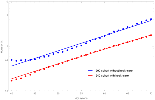
Figure 2: Mortality rates (log scale) at adults’ ages for the cohorts born in 1900 and 1940 in the UK. The dots are actual data (Berkeley Human Mortality Database) and the lines are model-implied mortality curves.

Figure 3(a) displays the model-implied optimal healthcare spending. In both countries, the proportion of wealth spent on healthcare is negligible at age 40, but increases to 0.5-1% at age 80. Figure 3(b) presents the calibrated efficacy function $g(h)=a\frac{h^{q}}{q}$ for the two countries. It particularly indicates that healthcare is more effective (in reducing mortality growth) in the UK than in the US. Along with Figure 3(a), we find that lower efficacy of healthcare is compensated by larger healthcare spending relative to wealth. That is, with enhanced efficacy, our model stipulates less healthcare spending, instead of more to exploit the reduced marginal cost to curtail mortality growth.

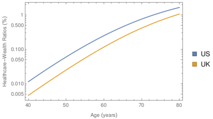
(a) Healthcare-wealth ratio (log scale) at adult ages.

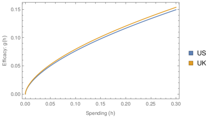
(b) Efficacy $g(h)$ given healthcare-wealth ratio $h$.

Figure 3: Calibrated healthcare-wealth ratio and efficacy of healthcare in the US and UK.

While Figure 3(b) hints at the potential of our model as a new analytic tool for healthcare efficacy, we stress that a more in-depth statistical and economic analysis is required here. First, one needs to find the confidence intervals for the estimated $(a,q)$, so as to test the hypothesis that the parameter differences across countries are statistically significant. Second, the economic interpretation of $q$ demands further investigation. While a higher $a$ unambiguously raises efficacy, the effect of $q$ is subtle: The efficacy increases faster with a lower $q$ when $h$ is small, but with a larger $q$ when $h$ is large. A careful analysis of these issues is well-warranted but beyond the scope of this paper, and we will leave it for future research.

Appendix A Proofs

A.1 Proof of Proposition 2.1

First, we assume that $\widetilde{V}$ is a $\mathbb{G}$-adapted semimartingale, with $\bar{\mathbb{E}}[\sup_{s\in[0,t]}|\widetilde{V}_{s}|]<\infty$ for all $t\geq 0$, that satisfies (2.6). Our goal is to show that $\widetilde{V}$ must be of the form (2.8). In view of (2.3) and (2.1), for any $0\leq t\leq s$, it holds for $\bar{\mathbb{P}}$-a.e. $\bar{\omega}=(\omega,\omega^{\prime})\in\bar{\Omega}$ that

$$\bar{\mathbb{P}}(\tau>\ell\mid\mathcal{F}_{s}\vee\mathcal{H}_{t})(\bar{\omega})=e^{-\int_{t}^{\ell}M_{u}^{h}(\omega)du}\mathbbm{1}_{\{\tau>t\}}(\bar{\omega}),\quad\forall t\leq\ell\leq s.$$ (A.1)

Also, since $\widetilde{V}$ is a $\mathbb{G}$-adapted semimartingale, it follows from (2.4) that there exists an $\mathbb{F}$-adapted semimartingale $V$ such that

$$\widetilde{V}_{t}=V_{t}\quad\hbox{$\bar{\mathbb{P}}$-a.s. on $\{t<\tau\}$},\qquad\forall t\geq 0.$$ (A.2)

Indeed, for any fixed $\omega\in\Omega$, consider $A_{t}(\omega):=\{\omega^{\prime}\in\Omega^{\prime}:t<\tau(\omega,\omega^{\prime})\}$ for all $t\geq 0$. As $\widetilde{V}$ is $\mathbb{G}$-adapted, (2.4) implies $\widetilde{V}_{t}(\omega,\omega^{\prime})$ is constant $\mathbb{P}^{\prime}$-a.s. on $A_{t}(\omega)$. By defining $V_{t}(\omega)=\widetilde{V}_{t}(\omega,\omega^{\prime})$, with $\omega^{\prime}\in A_{t}(\omega)$, for all $t\geq 0$, $V$ is an $\mathbb{F}$-adapted semimartingale satisfying (A.2). Also note that $\mathbb{E}[\sup_{s\in[0,t]}|V_{s}|]<\infty$, as $\bar{\mathbb{E}}[\sup_{s\in[0,t]}|\widetilde{V}_{s}|]<\infty$, for all $t\geq 0$. Now, observe that

$$\bar{\mathbb{E}}\left[\int_{t\wedge\tau}^{T\wedge\tau}f(c_{s},\widetilde{V}_{s}^{c,h})ds\ \middle|\ \mathcal{G}_{t}\right] =\bar{\mathbb{E}}\left[\int_{t}^{T}\mathbbm{1}_{\{s<\tau\}}f(c_{s},\widetilde{V}_{s}^{c,h})ds\ \middle|\ \mathcal{F}_{t}\vee\mathcal{H}_{t}\right]$$

$$=\int_{t}^{T}\bar{\mathbb{E}}\left[\mathbbm{1}_{\{s<\tau\}}f(c_{s},\widetilde{V}_{s}^{c,h})\ \middle|\ \mathcal{F}_{t}\vee\mathcal{H}_{t}\right]ds$$

$$=\int_{t}^{T}\bar{\mathbb{E}}\left[\bar{\mathbb{E}}\big{[}\mathbbm{1}_{\{s<\tau\}}f(c_{s},{V}_{s}^{c,h})\mid\mathcal{F}_{s}\vee\mathcal{H}_{t}\big{]}\ \middle|\ \mathcal{F}_{t}\vee\mathcal{H}_{t}\right]ds$$

$$=\int_{t}^{T}\bar{\mathbb{E}}\left[f(c_{s},{V}_{s}^{c,h})\ \bar{\mathbb{E}}\big{[}\mathbbm{1}_{\{s<\tau\}}\mid\mathcal{F}_{s}\vee\mathcal{H}_{t}\big{]}\ \middle|\ \mathcal{F}_{t}\vee\mathcal{H}_{t}\right]ds$$

$$=\int_{t}^{T}\bar{\mathbb{E}}\left[f(c_{s},{V}_{s}^{c,h})\mathbbm{1}_{\{t<\tau\}}e^{-\int_{t}^{s}M_{u}^{h}du}\ \middle|\ \mathcal{F}_{t}\vee\mathcal{H}_{t}\right]ds$$

$$=\bar{\mathbb{E}}\left[\int_{t}^{T}\mathbbm{1}_{\{t<\tau\}}e^{-\int_{t}^{s}M_{u}^{h}du}f(c_{s},{V}_{s}^{c,h})ds\ \middle|\ \mathcal{G}_{t}\right],$$ (A.3)

where the second and last equalities follow from Fubini’s theorem for conditional expectations (see [27, Theorem 27.17]), the third equality is due to the tower property of conditional expectations and (A.2), the fourth equality results from $c_{s}\in\mathcal{F}_{s}$ and $V^{c,h}_{s}\in\mathcal{F}_{s}$, and the fifth equality holds thanks to (A.1). Next, for $\bar{\mathbb{P}}$-a.e. fixed $\bar{\omega}=(\omega,\omega^{\prime})\in\bar{\Omega}$, consider the cumulative distribution function of $\tau$ given the information $\mathcal{F}_{T}\vee\mathcal{H}_{t}$, i.e.

$$F(s):=\bar{\mathbb{P}}(\tau\leq s\mid\mathcal{F}_{T}\vee\mathcal{H}_{t})(\bar{\omega}),\quad s\geq 0.$$

Thanks to (A.1), $F(s)=1-e^{-\int_{t}^{s}M_{u}^{h}(\omega)du}\mathbbm{1}_{\{\tau>t\}}(\bar{\omega})$ for $t\leq s\leq T$. This implies

$$\eta(s):=F^{\prime}(s)=M_{s}^{h}(\omega)e^{-\int_{t}^{s}M_{u}^{h}(\omega)du}\mathbbm{1}_{\{\tau>t\}}(\bar{\omega}),\quad\hbox{for}\ t\leq s\leq T,$$ (A.4)

which is the density function of $\tau$ given the information $\mathcal{F}_{T}\vee\mathcal{H}_{t}$. It follows that

$$\bar{\mathbb{E}}\left[\widetilde{V}_{\tau-}^{c,h}\mathbbm{1}_{\{\tau\leq T\}}\ \middle|\ \mathcal{G}_{t}\right] =\bar{\mathbb{E}}\left[{V}_{\tau-}^{c,h}\mathbbm{1}_{\{\tau\leq T\}}\ \middle|\ \mathcal{G}_{t}\right]\mathbbm{1}_{\{\tau\leq t\}}+\bar{\mathbb{E}}\left[{V}_{\tau-}^{c,h}\mathbbm{1}_{\{\tau\leq T\}}\ \middle|\ \mathcal{G}_{t}\right]\mathbbm{1}_{\{\tau>t\}}$$

$$={V}_{\tau-}^{c,h}\mathbbm{1}_{\{\tau\leq t\}}+\bar{\mathbb{E}}\left[\bar{\mathbb{E}}\big{[}{V}_{\tau-}^{c,h}\mathbbm{1}_{\{t<\tau\leq T\}}\mid\mathcal{F}_{T}\vee\mathcal{H}_{t}\big{]}\ \middle|\ \mathcal{F}_{t}\vee\mathcal{H}_{t}\right]$$

$$={V}_{\tau-}^{c,h}\mathbbm{1}_{\{\tau\leq t\}}+\bar{\mathbb{E}}\left[\int_{t}^{T}\mathbbm{1}_{\{t<\tau\}}M_{s}^{h}e^{-\int_{t}^{s}M_{u}^{h}du}{V}_{s}^{c,h}ds\ \middle|\ \mathcal{G}_{t}\right],$$ (A.5)

where the first line results from $\widetilde{V}_{\tau-}=V_{\tau-}$ (by (A.2)), the second line follows from the tower property of conditional expectations, and the third line is due to the density formula (A.4). Since $V$ is right-continuous, it has at most countably many jumps on $[t,T]$, so that we may use $V_{s}$ (instead of $V_{s-}$) in the last term of (A.5). Finally,

$$\bar{\mathbb{E}}\left[\widetilde{V}_{T}^{c,h}\mathbbm{1}_{\{\tau>T\}}\ \middle|\ \mathcal{G}_{t}\right]=\bar{\mathbb{E}}\left[\bar{\mathbb{E}}\big{[}{V}_{T}^{c,h}\mathbbm{1}_{\{\tau>T\}}\mid\mathcal{F}_{T}\vee\mathcal{H}_{t}\big{]}\ \middle|\ \mathcal{F}_{t}\vee\mathcal{H}_{t}\right]$$

$$\hskip 50.58878pt=\bar{\mathbb{E}}\left[{V}_{T}^{c,h}\bar{\mathbb{E}}\big{[}\mathbbm{1}_{\{\tau>T\}}\mid\mathcal{F}_{T}\vee\mathcal{H}_{t}\big{]}\ \middle|\ \mathcal{F}_{t}\vee\mathcal{H}_{t}\right]=\bar{\mathbb{E}}\left[\mathbbm{1}_{\{t<\tau\}}e^{-\int_{t}^{T}M_{u}^{h}du}{V}_{T}^{c,h}\ \middle|\ \mathcal{G}_{t}\right],$$ (A.6)

where the first equality follows from the tower property of conditional expectations and (A.2), the second equality is due to ${V}_{T}\in\mathcal{F}_{T}$, and the third equality is a consequence of (A.1). Now, combining (A.3), (A.5), and (A.6), we obtain from (2.6) and $\widetilde{V}_{\tau-}=V_{\tau-}$ that

$$\widetilde{V}_{t}^{c,h} =\mathbb{E}_{t}\bigg{[}\int_{t}^{T}e^{-\int_{t}^{s}M_{r}^{h}dr}\left(f(c_{s},{V}_{s}^{c,h})+\zeta^{1-\gamma}M_{s}^{h}{V}_{s}^{c,h}\right)ds+e^{-\int_{t}^{T}M_{s}^{h}ds}{V}_{T}^{c,h}\bigg{]}\mathbbm{1}_{\{t<\tau\}}$$

$$\hskip 202.35622pt+\zeta^{1-\gamma}{V}_{\tau-}^{c,h}\mathbbm{1}_{\{t\geq\tau\}},\ \ \text{ for all }0\leq t\leq T<\infty,$$ (A.7)

where we use the notation $\mathbb{E}_{t}\left[\cdot\right]=\mathbb{E}\left[\cdot|\mathcal{F}_{t}\right]$. This, together with (A.2), particularly implies

$$V_{t}(\omega)\mathbbm{1}_{\{t<\tau\}(\omega,\omega^{\prime})}=\widetilde{V}_{t}(\omega,\omega^{\prime})\mathbbm{1}_{\{t<\tau\}(\omega,\omega^{\prime})}=E_{t,T}(\omega)\mathbbm{1}_{\{t<\tau\}(\omega,\omega^{\prime})},$$ (A.8)

where

$$E_{t,T}(\omega):=\mathbb{E}_{t}\bigg{[}\int_{t}^{T}e^{-\int_{t}^{s}M_{r}^{h}dr}\left(f(c_{s},{V}_{s}^{c,h})+\zeta^{1-\gamma}M_{s}^{h}{V}_{s}^{c,h}\right)ds+e^{-\int_{t}^{T}M_{s}^{h}ds}{V}_{T}^{c,h}\bigg{]}(\omega).$$

For any $\omega\in\Omega$, since there exists $\omega^{\prime}\in\Omega^{\prime}$ such that $\mathbbm{1}_{\{t<\tau\}(\omega,\omega^{\prime})}=1$ (in view of (2.3) and (2.1)), we conclude from (A.8) that $V_{t}(\omega)=E_{t,T}(\omega)$. We can then simplify (A.7) as

$$\widetilde{V}_{t} =V_{t}\mathbbm{1}_{\{t<\tau\}}+\zeta^{1-\gamma}{V}_{\tau-}\mathbbm{1}_{\{t\geq\tau\}},$$ (A.9)

where $V$ satisfies

$$V_{t}=\mathbb{E}_{t}\bigg{[}\int_{t}^{T}e^{-\int_{t}^{s}M_{r}^{h}dr}\left(f(c_{s},{V}_{s})+\zeta^{1-\gamma}M_{s}^{h}{V}_{s}\right)ds+e^{-\int_{t}^{T}M_{s}^{h}ds}{V}_{T}\bigg{]},\ \ \forall 0\leq t\leq T<\infty$$ (A.10)

Now, note that the above equation directly implies

$$V^{\prime}_{t}:=e^{-\int_{0}^{t}M_{r}^{h}dr}V_{t}=\mathscr{M}^{\prime}_{t}-\int_{0}^{t}e^{-\int_{0}^{s}M_{r}^{h}dr}\left(f(c_{s},{V}_{s})+\zeta^{1-\gamma}M_{s}^{h}{V}_{s}\right)ds,$$

where

$$\mathscr{M}^{\prime}_{t}:=\mathbb{E}_{t}\bigg{[}\int_{0}^{T}e^{-\int_{0}^{s}M_{r}^{h}dr}\left(f(c_{s},{V}_{s})+\zeta^{1-\gamma}M_{s}^{h}{V}_{s}\right)ds+e^{-\int_{0}^{T}M_{s}^{h}ds}{V}_{T}\bigg{]}$$

is an $\mathbb{F}$-martingale on $[0,T]$, thanks to (A.10). Applying generalized Itô’s formula for semimartingales (see [20, Theorem I.4.57]) to $V_{t}=e^{\int_{0}^{t}M_{r}^{h}dr}V^{\prime}_{t}$ gives $dV_{t}=-F(c_{t},M^{h}_{t},V_{t})+e^{\int_{0}^{t}M_{r}^{h}dr}d\mathscr{M}^{\prime}_{t}.$ Since $0\leq M^{h}_{t}\leq me^{\beta t}$ by definition (by (2.2)), $\mathscr{M}_{t}:=\int_{0}^{t}e^{\int_{0}^{s}M_{r}^{h}dr}d\mathscr{M}^{\prime}_{s}$ is again an $\mathbb{F}$-martingale. Hence, $V$ is a solution to BSDE (2.9). This, together with (A.9), yields the desired result.

Next, we prove the converse, i.e. a process $\widetilde{V}$ given by (2.8) has the three properties: (i) it is a $\mathbb{G}$-adapted semimartingale; (ii) $\bar{\mathbb{E}}[\sup_{s\in[0,t]}|\widetilde{V}_{s}|]<\infty$ for all $t\geq 0$; (iii) it satisfies (2.6). By the construction in (2.8), properties (i) and (ii) follow directly from $V$ being an $\mathbb{F}$-adapted semimartingale with $\mathbb{E}[\sup_{s\in[0,t]}|V_{s}|]<\infty$ for all $t\geq 0$. Now, by applying generalized Itô’s formula for semimartingales (see [20, Theorem I.4.57]) to $e^{-\int_{0}^{t}M_{s}^{h}ds}V_{t}$, we see that $V$ satisfies (A.10). This, together with the same arguments in (A.3), (A.5), and (A.6), shows that $\widetilde{V}$ in (2.8) satisfies (2.6).

A.2 Derivation of Proposition 2.2

Lemma A.1.

Let $c,h,V$ and $W$ be $\mathbb{F}$-progressively measurable processes with $W_{s}\leq V_{s}$ for all $s\geq 0$. If there exists $k\in\mathbb{R}$ such that $V$ satisfies (2.12), then

$$F(c_{s},M^{h}_{s},V_{s})-F(c_{s},M^{h}_{s},W_{s})\leq-\Gamma(\Lambda,M^{h}_{s})(V_{s}-W_{s}),$$ (A.11)

where $F$ is given in (2.10), $\Lambda:=\delta\theta+(1-\theta)k$ (as in Definition 2.2), and $\Gamma$ is defined by

$$\Gamma(\lambda,m):=\lambda+\frac{\gamma(\psi-1)}{1-\gamma}(1-\zeta^{1-\gamma})m.$$ (A.12)

Proof.

As in the proof of [24, Lemma B.1], (A.11) holds by the mean value theorem provided that $F_{v}(c_{s},M^{h}_{s},u)\leq-\Gamma(\Lambda,M^{h}_{s})$ for all $u\in[W_{s},V_{s}]$. To this end, note that

$$F_{v}(c_{s},M^{h}_{s},u)=-\bigg{(}\delta\theta+(1-\zeta^{1-\gamma})M^{h}_{s}+\delta(1-\theta)\bigg{(}\frac{c_{s}^{1-\gamma}}{(1-\gamma)u}\bigg{)}^{{1}/{\theta}}\bigg{)}.$$

Thanks to Assumption 1, a direct calculation shows $F_{vv}(c_{s},M^{h}_{s},u)>0$, i.e. $F_{v}(c_{s},M^{h}_{s},u)$ is increasing in $u$. This, together with $V$ satisfying (2.12), implies that for all $u\in[W_{s},V_{s}]$, $F_{v}(c_{s},M^{h}_{s},u)\leq F_{v}(c_{s},M^{h}_{s},\hat{u})$, where $\hat{u}:=\delta^{\theta}\big{(}k-\frac{\psi-1}{1-\gamma}(\zeta^{1-\gamma}-1)M^{h}_{s}\big{)}^{-\theta}\frac{c_{s}^{1-\gamma}}{1-\gamma}$. By direct calculation,

$$F_{v}(c_{s},M^{h}_{s},\hat{u}) =-\bigg{(}\delta\theta+(1-\zeta^{1-\gamma})M^{h}_{s}+(1-\theta)\left(k-\frac{\psi-1}{1-\gamma}(\zeta^{1-\gamma}-1)M^{h}_{s}\right)\bigg{)}$$

$$=-\left(\Lambda+\frac{\gamma(\psi-1)}{1-\gamma}(1-\zeta^{1-\gamma})M^{h}_{s}\right)=-\Gamma(\Lambda,M^{h}_{s}),$$

where the second equality follows from the definition of $\Lambda$ and $\theta=\frac{1-\gamma}{1-1/\psi}$. ∎

To prove Proposition 2.2, we intend to follow the idea in the proof of [24, Theorem 2.2]. The involvement of the controlled mortality $M^{h}$ in (2.11), as well as the possibility that $\Lambda$ therein can be negative (Remark 2.5), result in additional technicalities. The proof below combines arguments in [24, Theorem 2.2] and [12, Theorem 2.1], adapted to weaker regularity of processes.

Proof of Proposition 2.2.

Recall the function $\Gamma$ in (A.12). Fix $0\leq t_{0}<T$, define

$$\Delta_{t}:=e^{-\int_{t_{0}}^{t}\Gamma(0,M^{h}_{s})ds}\left(V_{t}^{1}-V_{t}^{2}\right),\quad t\in[t_{0},T],$$ (A.13)

and consider the stopping time $\theta:=\inf\left\{s\geq t_{0}:V_{s}^{1}\leq V_{s}^{2}\right\}$. Applying generalized Itô’s formula (see [20, Theorem I.4.57]) to $e^{-\int_{0}^{t}\Gamma(0,M^{h}_{s})ds}V_{t}^{i}$, $i=1,2$, yields

$$d\left(e^{-\int_{0}^{t}\Gamma(0,M^{h}_{s})ds}V_{t}^{1}\right) =-e^{-\int_{0}^{t}\Gamma(0,M^{h}_{s})ds}\left[\Gamma(0,M^{h}_{s})V_{t}^{1}+F(c_{t},M^{h}_{t},V_{t}^{1})\right]dt+e^{-\int_{0}^{t}\Gamma(0,M^{h}_{s})ds}d\mathscr{M}_{t}^{1},$$

$$d\left(e^{-\int_{0}^{t}\Gamma(0,M^{h}_{s})ds}V_{t}^{2}\right) =-e^{-\int_{0}^{t}\Gamma(0,M^{h}_{s})ds}\left[\Gamma(0,M^{h}_{s})V_{t}^{2}+G(t,V_{t}^{2})\right]dt+e^{-\int_{0}^{t}\Gamma(0,M^{h}_{s})ds}d\mathscr{M}_{t}^{2},$$

where $\mathscr{M}^{1}$, $\mathscr{M}^{2}$ are some $\mathbb{F}$-martingales on $[0,T]$. As $0\leq\Gamma(0,M^{h}_{t})\leq\frac{\gamma(\psi-1)}{1-\gamma}(1-\zeta^{1-\gamma})me^{\beta t}$ by the definition of $M^{h}$ in (2.2), $r\mapsto\int_{t_{0}}^{r}e^{-\int_{0}^{t}\Gamma(0,M^{h}_{s})ds}d\mathscr{M}_{t}^{i}$ is a true martingale for $i=1,2$. Hence,

$$\Delta_{t}=\mathbb{E}_{t}\left[\int_{t}^{T}\mathbbm{1}_{\{s<\theta\}}\left[\left(F(c_{s},M^{h}_{s},V_{s}^{1})-G(s,V_{s}^{2})\right)+\Gamma(0,M^{h}_{s})\left(V_{s}^{1}-V_{s}^{2}\right)\right]e^{-\int_{t_{0}}^{s}\Gamma(0,M^{h}_{r})dr}ds+\Delta_{T\wedge\theta}\right].$$

Observe that

$$\mathbbm{1}_{\{s<\theta\}}\left(F(c_{s},M^{h}_{s},V_{s}^{1})-G(s,V_{s}^{2})\right) =\mathbbm{1}_{\{s<\theta\}}\left(F(c_{s},M^{h}_{s},V_{s}^{1})-F(c_{s},M^{h}_{s},V_{s}^{2})\right)$$

$$\hskip 36.135pt+\mathbbm{1}_{\{s<\theta\}}\left(F(c_{s},M^{h}_{s},V_{s}^{2})-G(s,V_{s}^{2})\right)$$

$$\leq\mathbbm{1}_{\{s<\theta\}}\left(F(c_{s},M^{h}_{s},V_{s}^{1})-F(c_{s},M^{h}_{s},V_{s}^{2})\right)$$

$$\leq\mathbbm{1}_{\{s<\theta\}}\left(-\Gamma(\Lambda,M^{h}_{s})\left(V_{s}^{1}-V_{s}^{2}\right)\right),$$

where the first inequality follows from $F(c_{s},M^{h}_{s},V_{s}^{2})\leq G(s,V_{s}^{2})$, and the second is due to Lemma A.1, which is applicable here as $V_{s}^{1}>V_{s}^{2}$ for $s\in[t,\theta)$. Thanks to the above inequality,

$$\Delta_{t} \leq\mathbb{E}_{t}\left[\int_{t}^{T}\mathbbm{1}_{\{s<\theta\}}\left[-\Gamma(\Lambda,M^{h}_{s})+\Gamma(0,M^{h}_{s})\right]\left(V_{s}^{1}-V_{s}^{2}\right)e^{-\int_{t_{0}}^{s}\Gamma(0,M^{h}_{r})dr}ds+\Delta_{T\wedge\theta}\right]$$

$$=\mathbb{E}_{t}\left[-\int_{t}^{T}\mathbbm{1}_{\{s<\theta\}}\Lambda\Delta_{s}ds+\Delta_{T\wedge\theta}\right],$$ (A.14)

where the second line follows from $\Gamma(\Lambda,M^{h}_{s})=\Lambda+\Gamma(0,M^{h}_{s})$ and (A.13). Multiplying both sides by $\mathbbm{1}_{\{t<\theta\}}$ yields

$$\Delta_{t}\mathbbm{1}_{\{t<\theta\}}\leq\mathbb{E}_{t}\left[-\int_{t}^{T}\Lambda\Delta_{s}\mathbbm{1}_{\{s<\theta\}}ds+\Delta_{T\wedge\theta}\mathbbm{1}_{\{t<\theta\}}\right]\leq\mathbb{E}_{t}\left[-\int_{t}^{T}\Lambda\Delta_{s}\mathbbm{1}_{\{s<\theta\}}ds+\Delta_{T}\mathbbm{1}_{\{T<\theta\}}\right],$$

where the second inequality follows from the right continuity of $V^{1}$ and $V^{2}$. Indeed, the right continuity implies $V_{\theta}^{1}\leq V_{\theta}^{2}$, so that $\Delta_{T\wedge\theta}=\Delta_{\theta}\mathbbm{1}_{\{\theta\leq T\}}+\Delta_{T}\mathbbm{1}_{\{T<\theta\}}\leq\Delta_{T}\mathbbm{1}_{\{T<\theta\}}$. Set $\Delta_{t}^{+}:=\Delta_{t}\mathbbm{1}_{\{t<\theta\}}$, and write the previous inequality as $\Delta_{t}^{+}\leq\mathbb{E}_{t}\big{[}-\int_{t}^{T}\Lambda\Delta_{s}^{+}ds+\Delta_{T}^{+}\big{]}.$ Taking expectations on both sides and using Fubini’s theorem give

$$\Theta_{t}\leq-\int_{t}^{T}\Lambda\Theta_{s}ds+\Theta_{T},$$ (A.15)

where $\Theta_{t}:=\mathbb{E}\left[\Delta^{+}_{t}\right]\geq 0$ is well-defined as $\Gamma(0,M_{s})\geq 0$ and $\mathbb{E}\big{[}\sup_{t\in[0,T]}|V_{t}^{i}|\big{]}<\infty$, thanks to $V^{i}\in\mathcal{E}^{h}_{k}$ (Definition 2.2), for $i=1,2$. Now, if $\Lambda>0$, by writing $\Theta_{T}\geq\Theta_{t}+\int_{t}^{T}\Lambda\Theta_{s}ds$, we apply standard Gronwall’s inequality to get $\Theta_{T}\geq\Theta_{t}e^{\int_{t}^{T}\Lambda ds}$, or equivalently

$$\Theta_{t}\leq\Theta_{T}e^{-\int_{t}^{T}\Lambda ds},\quad t\in[t_{0},T].$$ (A.16)

If $\Lambda<0$, applying backward Gronwall’s inequality (see [33, Proposition 2]) to (A.15) also gives (A.16). By (A.16), (A.13), and (A.12), we obtain

$$\Theta_{t_{0}}\leq\Theta_{T}e^{-\int_{t_{0}}^{T}\Lambda ds}\leq\mathbb{E}\left[e^{-\int_{t_{0}}^{T}\Gamma(\Lambda,M_{s})ds}\left(|V_{T}^{1}|+|V_{T}^{2}|\right)\right].$$ (A.17)

Since $T>0$ is arbitrary, the transversality condition in $\eqref{TransversalityCondition}$ for $V_{t}^{1}$ and $V_{t}^{2}$ immediately implies

$$0\leq\Theta_{t_{0}}\leq\lim\limits_{T\rightarrow\infty}\mathbb{E}\left[e^{-\int_{t_{0}}^{T}\Gamma(\Lambda,M_{s})ds}\left(|V_{T}^{1}|+|V_{T}^{2}|\right)\right]=0.$$ (A.18)

That is, $\Theta_{t_{0}}=\mathbb{E}\left[\left(V_{t_{0}}^{1}-V_{t_{0}}^{2}\right)1_{\{t_{0}<\theta\}}\right]=0$. This entails $\theta=t_{0}$, and thus $V_{t_{0}}^{1}\leq V_{t_{0}}^{2}$. Since $t_{0}\geq 0$ is arbitrary, we conclude that $V_{t}^{1}\leq V_{t}^{2}$ for all $t\geq 0$. ∎

A.3 Proof of Proposition 4.1

For any fixed $m>0$ such that $\tilde{c}_{0}(m)>0$, define $w(x):=\delta^{\theta}\frac{x^{1-\gamma}}{1-\gamma}\tilde{c}_{0}(m)^{-\frac{\theta}{\psi}}$ for $x>0$. In order to apply Theorem 3.1, we need to verify all its conditions. It can be checked directly that $w$, as a one-variable function, solves (3.1) in a trivial way, with all derivatives in $m$ being zero. For any $(c,\pi,h)\in\mathcal{P}=\mathcal{P}_{1}$, since $(X^{c,\pi,h})^{1-\gamma}$ satisfies (2.11) (with $\Lambda^{*}$ in place of $\Lambda$), so does $w(X^{c,\pi,h}_{t})$, i.e. $w(X^{c,\pi,h}_{t})\in\mathcal{E}^{h}_{k^{*}}$. By the definitions of $\mathcal{P}$ and $w$, $\mathcal{P}=\mathcal{P}_{1}\subseteq\mathcal{H}_{k^{*}}$ and (3.10) is satisfied. As $\tilde{c}_{0}(m)>0$, $w_{x}>0$ and $w_{xx}<0$ by definition. It follows that $\bar{c}(x,m):=x\tilde{c}_{0}(m)$ and $\bar{\pi}(x,m):=\frac{\mu}{\gamma\sigma^{2}}$ are unique maximizers of the supremums in (3.11), respectively. The supremum in (3.12) is zero, as $g\equiv 0$ and $w_{x}>0$. Hence, $\bar{h}(x,m):=0$ trivially maximizes (3.12). The only condition that remains to be checked is “$(c^{*},\pi^{*},h^{*})$ in (3.13) belongs to $\mathcal{P}$ and $W^{*}_{t}:=w(X^{c^{*},\pi^{*},h^{*}}_{t})$ satisfies (2.12)”.

Observe that a unique solution $X^{*}=X^{c^{*},\pi^{*},h^{*}}$ to (3.2) exists as a geometric Brownian motion

$$dX_{t}^{*}=X_{t}^{*}\left(r+\frac{1}{\gamma}\left(\frac{\mu}{\sigma}\right)^{2}-\tilde{c}_{0}(m)\right)dt+X_{t}^{*}\frac{\mu}{\gamma\sigma}dB_{t},$$ (A.19)

This implies that

$$(X^{*}_{t})^{1-\gamma}=x^{1-\gamma}\text{exp}\left((1-\gamma)\left(r+\frac{1}{2\gamma}\left(\frac{\mu}{\sigma}\right)^{2}-\tilde{c}_{0}(m)-\frac{(1-\gamma)}{2\gamma^{2}}\left(\frac{\mu}{\sigma}\right)^{2}\right)t+\frac{(1-\gamma)\mu}{\gamma\sigma}B_{t}\right),$$ (A.20)

which is again a geometric Brownian motion that satisfies the dynamics

$$\frac{dY_{t}}{Y_{t}}=(1-\gamma)\left(r+\frac{1}{2\gamma}\left(\frac{\mu}{\sigma}\right)^{2}-\tilde{c}_{0}(m)\right)dt+\frac{(1-\gamma)\mu}{\gamma\sigma}dB_{t},\quad Y_{0}=x^{1-\gamma}.$$

Consequently,

$$e^{-\Lambda^{*}t}\mathbb{E}\left[e^{-\gamma(\psi-1)\frac{1-\zeta^{1-\gamma}}{1-\gamma}mt}(X^{*}_{t})^{1-\gamma}\right]=x^{1-\gamma}e^{(C-\Lambda^{*})t},$$ (A.21)

where

$$C:=(1-\gamma)\left(r+\frac{1}{2\gamma}\left(\frac{\mu}{\sigma}\right)^{2}-\tilde{c}_{0}(m)\right)-\gamma(\psi-1)\frac{1-\zeta^{1-\gamma}}{1-\gamma}m.$$

Remarkably, by the definitions of $\tilde{c}_{0}(m)$ and $\Lambda^{*}$ in (3.18) and (4.2), a direct calculation shows that $C-\Lambda^{*}=-\tilde{c}_{0}(m)<0$, where the inequality follows from $\tilde{c}_{0}(m)>0$. It follows from (A.21) that

$$\lim_{t\to\infty}e^{-\Lambda^{*}t}\mathbb{E}\left[e^{-\gamma(\psi-1)\frac{1-\zeta^{1-\gamma}}{1-\gamma}mt}(X^{*}_{t})^{1-\gamma}\right]=0.$$ (A.22)

On the other hand, we can rewrite (A.20) as

$$(X^{*}_{t})^{1-\gamma}=x^{1-\gamma}\text{exp}\left((1-\gamma)\left(r+\frac{1}{2\gamma}\left(\frac{\mu}{\sigma}\right)^{2}-\tilde{c}_{0}(m)\right)t\right)\cdot Z_{t},$$ (A.23)

where $Z$ is a geometric Brownian motion with the dynamics ${dZ_{t}}=Z_{t}\frac{(1-\gamma)\mu}{\gamma\sigma}dB_{t}$, $Z_{0}=1$. As $Z$ is a martingale, we can apply the Burkhölder-Davis-Gundy inequality to get

$$\mathbb{E}\bigg{[}\sup\limits_{s\in[0,t]}(X_{s}^{*})^{1-\gamma}\bigg{]}\leq Kx^{1-\gamma}e^{\left(|1-\gamma|\left|r+\frac{1}{2\gamma}\left(\frac{\mu}{\sigma}\right)^{2}-\tilde{c}_{0}(m)\right|\right)t}\frac{|1-\gamma|\mu}{\gamma\sigma}\mathbb{E}\left[\bigg{(}\int_{0}^{t}Z_{s}^{2}ds\bigg{)}^{1/2}\right],$$ (A.24)

for some constant $K>0$. By Jensen’s inequality and Fubini’s theorem,

$$\mathbb{E}\bigg{[}\bigg{(}\int_{0}^{t}Z_{s}^{2}ds\bigg{)}^{1/2}\bigg{]}\leq\bigg{(}\int_{0}^{t}\mathbb{E}[Z_{s}^{2}]ds\bigg{)}^{1/2}=\bigg{(}\int_{0}^{t}e^{\frac{(1-\gamma)^{2}\mu^{2}}{\gamma^{2}\sigma^{2}}s}ds\bigg{)}^{1/2}=\frac{\gamma\sigma}{|1-\gamma|\mu}\bigg{(}e^{\frac{(1-\gamma)^{2}\mu^{2}}{\gamma^{2}\sigma^{2}}t}-1\bigg{)}^{1/2}.$$

We then conclude from the above two inequalities that

$$\mathbb{E}\bigg{[}\sup\limits_{s\in[0,t]}(X_{s}^{*})^{1-\gamma}\bigg{]}<\infty,\quad\forall t\geq 0.$$ (A.25)

By (A.22) and (A.25), $(X^{*})^{1-\gamma}$ satisfies (2.11) (with $\Lambda^{*}$ in place of $\Lambda$), and so does the process $W^{*}_{t}:=w(X^{*}_{t})=\delta^{\theta}\tilde{c}_{0}(m)^{-\frac{\theta}{\psi}}\frac{(X^{*}_{t})^{1-\gamma}}{1-\gamma}$, i.e. $W^{*}\in\mathcal{E}^{h^{*}}_{k^{*}}$. By applying Itô’s formula to $W^{*}_{t}$ and noting

$$\mathbb{E}\bigg{[}\sup_{s\in[0,t]}\pi^{*}_{s}(X_{s}^{*})^{1-\gamma}\bigg{]}<\infty\quad\hbox{for all}\ t\geq 0,$$ (A.26)

a consequence of (A.25) and $\pi^{*}_{t}\equiv\frac{\mu}{\gamma\sigma^{2}}$, we argue as in the proof of Theorem 3.1 that $W^{*}_{t}$ is a solution to (2.9). Moreover,

$$W^{*}_{t}=\delta^{\theta}\tilde{c}_{0}(m)^{-\theta+(1-\gamma)}\frac{(X^{*}_{t})^{1-\gamma}}{1-\gamma}=\delta^{\theta}\tilde{c}_{0}(m)^{-\theta}\frac{(c^{*}_{t})^{1-\gamma}}{1-\gamma}$$

By (4.8), this shows that $W^{*}$ satisfies (2.12) with $k=k^{*}$. Hence, $(c^{*},h^{*})$ is $k^{*}$-admissible, so that we can conclude $(c^{*},\pi^{*},h^{*})\in\mathcal{P}$. Theorem 3.1 is then applicable, asserting that $w(x,m)=v(x,m)$ and $(c^{*},\pi^{*},h^{*})$ optimizes (3.5).

A.4 Proof of Theorem 4.1

Define $w(x,m):=\delta^{\theta}\frac{x^{1-\gamma}}{1-\gamma}u^{*}(m)^{-\frac{\theta}{\psi}}$ for $(x,m)\in\mathbb{R}^{2}_{+}$. To apply Theorem 3.1, we need to verify all its conditions. It can be checked, as in (3.15)-(3.17), that $w\in C^{2,1}(\mathbb{R}_{+}\times\mathbb{R}_{+})$ solves (3.1). By the definitions of $\mathcal{P}$ and $w$, $\mathcal{P}\subseteq\mathcal{H}_{k^{*}}$ and (3.10) is satisfied for any $(c,\pi,h)\in\mathcal{P}$. As $w_{x}>0$, $w_{xx}<0$, and $g$ satisfies Assumption 2, $\bar{c}$, $\bar{\pi}$, and $\bar{h}$ in (3.19) are unique maximizers of the supermums in (3.11) and (3.12). It remain to show (i) for any $(c,\pi,h)\in\mathcal{P}$, $w(X^{c,\pi,h}_{t},M^{h}_{t})\in\mathcal{E}^{h}_{k^{*}}$; (ii) $(c^{*},\pi^{*},h^{*})$, defined using $\bar{c}$, $\bar{\pi}$, and $\bar{h}$ as in (3.13), belongs to $\mathcal{P}$ and $W^{*}_{t}:=w(X^{c^{*},\pi^{*},h^{*}}_{t},M^{h^{*}}_{t})$ satisfies (2.12).

(i) Take any $\mathfrak{p}=(c,\pi,h)\in\mathcal{P}$, and set $W_{t}:=w(X_{t}^{\mathfrak{p}},M_{t}^{h})$ for $t\geq 0$. We will prove $W\in\mathcal{E}^{h}_{k^{*}}$.

• Case (i)-1: $\gamma\in(\frac{1}{\psi},1)$. In view of (4.11), (3.18), and (4.1), we have $u^{*}(m)\geq\tilde{c}_{0}(m)\geq\tilde{c}_{0}(0)=k^{*}>0$. As $\theta>0$ when $\gamma\in(\frac{1}{\psi},1)$, this implies

  $$0<W_{t}=\delta^{\theta}\frac{(X^{\mathfrak{p}}_{t})^{1-\gamma}}{1-\gamma}u^{*}(M^{h}_{t})^{-\frac{\theta}{\psi}}\leq\delta^{\theta}\frac{(X^{\mathfrak{p}}_{t})^{1-\gamma}}{1-\gamma}(k^{*})^{-\frac{\theta}{\psi}}\quad\forall t\geq 0,$$

  Since $(X^{\mathfrak{p}})^{1-\gamma}$ satisfies (2.11) (as $\mathfrak{p}\in\mathcal{P}=\mathcal{P}_{1}$), the above implies that $W$ also satisfies (2.11).

• Case (i)-2: $\gamma>1$ and $\zeta<1$. As $\mathfrak{p}\in\mathcal{P}=\mathcal{P}_{2}$, there exists $\eta\in(1-\frac{1}{\gamma},1)$ such that (4.3) holds. Consider

  $$\alpha:=-\eta\frac{\gamma(\psi-1)}{1-\gamma}(\zeta^{1-\gamma}-1)>0,\qquad\alpha^{\prime}:=-(1-\eta)\frac{\gamma(\psi-1)}{1-\gamma}(\zeta^{1-\gamma}-1)>0,$$ (A.27)

  $$F_{t}:=\left(u_{\beta}(M_{t}^{h})\right)^{-\frac{\theta}{\psi}}\text{exp}\left(-\alpha^{\prime}\int_{0}^{t}M_{s}^{h}ds\right)\quad\hbox{for}\ t\geq 0.$$ (A.28)

  First, we claim that the process $F$ is bounded from above; more specifically,

  $$\sup_{t\geq 0}F_{t}\leq u_{\beta}\left(-\frac{\theta}{\alpha^{\prime}\psi}\beta\right)^{-{\theta}/{\psi}}<\infty.$$ (A.29)

  Observe that

  $$\frac{dF_{t}}{dt} =-\left(\alpha^{\prime}M_{t}^{h}+\frac{\theta}{\psi}u_{\beta}(M_{t}^{h})^{-1}u_{\beta}^{\prime}(M_{t}^{h})\frac{dM_{t}^{h}}{dt}\right)F_{t}$$

  $$=-\left(\alpha^{\prime}M_{t}^{h}+\frac{\theta}{\psi\beta}(\beta-g(h_{t}))\big{[}u_{\beta}(M_{t}^{h})-\tilde{c}_{0}(M_{t}^{h})\big{]}\right)F_{t},$$ (A.30)

  where the second equality follows as $u_{\beta}$ solves (4.6) with $\ell=\beta$. For each $\omega\in\Omega$, consider

  $$S(\omega):=\left\{t\geq 0:M_{t}^{h}(\omega)=\frac{-\theta}{\alpha^{\prime}\psi\beta}(\beta-g(h_{t}))\big{(}u_{\beta}(M_{t}^{h})-\tilde{c}_{0}(M_{t}^{h})\big{)}(\omega)\right\}.$$

  We deduce from (A.30) that local maximizers of $t\mapsto F_{t}(\omega)$ must belong to $S(\omega)$, i.e.

  $$\hbox{if $t\geq 0$ satisfies}\ F_{t}(\omega)=\max_{s\in[(t-\varepsilon)^{+},t+\varepsilon]}F_{s}(\omega)\ \hbox{for some $\varepsilon>0$, then $t\in S(\omega)$}.$$ (A.31)

  Also, by $g\geq 0$ and (4.7),

  $$L_{t}(\omega):=\frac{-\theta}{\alpha^{\prime}\psi\beta}(\beta-g(h_{t}))\big{(}u_{\beta}(M_{t}^{h})-\tilde{c}_{0}(M_{t}^{h})\big{)}(\omega)\leq-\frac{\theta}{\alpha^{\prime}\psi}\beta,\quad\forall t\geq 0.$$ (A.32)

  This particularly implies that

  $$M^{h}_{t}(\omega)=L_{t}(\omega)\leq-\frac{\theta}{\alpha^{\prime}\psi}\beta,\quad\hbox{for each}\ t\in S(\omega).$$ (A.33)

  Now, there are three distinct possibilities: 1) There exists $t^{*}\geq 0$ such that $M^{h}_{t}(\omega)<L_{t}(\omega)$ for all $t>t^{*}$. Then, $S(\omega)\subseteq[0,t^{*}]$ and (A.32) implies $M^{h}_{t}(\omega)<-\frac{\theta}{\alpha^{\prime}\psi}\beta$ for all $t>t^{*}$. It then follows from (A.31) and (A.28) that

  $$\sup_{t\leq t^{*}}F_{t}(\omega)=\sup_{t\in S(\omega)}F_{t}(\omega)\leq\sup_{t\in S(\omega)}u_{\beta}\big{(}M^{h}_{t}(\omega)\big{)}^{-\frac{\theta}{\psi}}\leq u_{\beta}\left(-\frac{\theta}{\alpha^{\prime}\psi}\beta\right)^{-{\theta}/{\psi}},$$ (A.34)

  where the last inequality follows from (A.33). Moreover,

  $$\sup_{t>t^{*}}F_{t}(\omega)\leq\sup_{t>t^{*}}u_{\beta}\big{(}M^{h}_{t}(\omega)\big{)}^{-\frac{\theta}{\psi}}\leq u_{\beta}\left(-\frac{\theta}{\alpha^{\prime}\psi}\beta\right)^{-{\theta}/{\psi}},$$

  i.e. (A.29) holds. 2) There exists $t^{*}\geq 0$ such that $M^{h}_{t}(\omega)>L_{t}(\omega)$ for all $t>t^{*}$. By (A.30), $F_{t}(\omega)$ is strictly decreasing for $t>t^{*}$. Thus, $\sup_{t\geq 0}F_{t}(\omega)=\sup_{t\leq t^{*}}F_{t}(\omega)=\sup_{t\in S(\omega)}F_{t}(\omega)$. By the estimate in (A.34), (A.29) holds. 3) Neither 1) nor 2) above holds. This entails $\sup\{t\geq 0:t\in S(\omega)\}=\infty$. Hence, $\sup_{t\geq 0}F_{t}(\omega)=\sup_{t\in S(\omega)}F_{t}(\omega)$, so that (A.29) holds by the estimate in (A.34). Now, since $u^{*}\leq u_{\beta}$ (by (4.11)), $-\theta/\psi>0$, and $1-\gamma<0$,

  $$0 \geq e^{\frac{\gamma(\psi-1)}{1-\gamma}(\zeta^{1-\gamma}-1)\int_{0}^{t}M^{h}_{s}ds}W_{t}\geq\delta^{\theta}\left(u_{\beta}(M_{t}^{h})\right)^{-{\theta}/{\psi}}e^{\frac{\gamma(\psi-1)}{1-\gamma}(\zeta^{1-\gamma}-1)\int_{0}^{t}M^{h}_{s}ds}\frac{(X_{t}^{\mathfrak{p}})^{1-\gamma}}{1-\gamma}$$

  $$=\delta^{\theta}F_{t}\ e^{-\alpha\int_{0}^{t}M^{h}_{s}ds}\frac{(X_{t}^{\mathfrak{p}})^{1-\gamma}}{1-\gamma}\geq\delta^{\theta}u_{\beta}\left(\frac{-\theta}{\alpha^{\prime}\psi}\beta\right)^{-{\theta}/{\psi}}e^{-\alpha\int_{0}^{t}M^{h}_{s}ds}\frac{(X_{t}^{\mathfrak{p}})^{1-\gamma}}{1-\gamma},$$

  where the equality follows from (A.28) and (A.27), and the last inequality is due to (A.29). Recalling that $\mathfrak{p}\in\mathcal{P}=\mathcal{P}_{2}$, we conclude from (4.3) and the above inequality that

  $$\lim\limits_{t\rightarrow\infty}e^{-\Lambda^{*}t}\mathbb{E}\bigg{[}e^{\frac{\gamma(\psi-1)}{1-\gamma}(\zeta^{1-\gamma}-1)\int_{0}^{t}M_{s}^{h}ds}W_{t}\bigg{]}=0.$$

  On the other hand, since $M_{t}^{h}\leq me^{\beta t}$,

  $$\mathbb{E}\bigg{[}\sup\limits_{s\in[0,t]}|W_{t}|\bigg{]}\leq\frac{\delta^{\theta}}{|1-\gamma|}u_{\beta}(me^{\beta t})^{-\theta/\psi}\mathbb{E}\bigg{[}\sup_{s\in[0,t]}(X_{s}^{\mathfrak{p}})^{1-\gamma}\bigg{]}<\infty,\quad\forall t\geq 0.$$

  where the finiteness is a direct consequence of $\mathfrak{p}\in\mathcal{P}$.

• Case (i)-3: $\gamma>1$ and $\zeta=1$. In view of (4.5), $u_{\ell}\equiv k^{*}>0$ for any $\ell>0$. It then follows from (4.11) that $u^{*}\equiv k^{*}>0$. The required properties then follow directly from $\mathfrak{p}\in\mathcal{P}=\mathcal{P}_{1}$.

(ii) Now, we show that $(c^{*},\pi^{*},h^{*})\in\mathcal{P}$ and $W^{*}_{t}:=w(X^{c^{*},\pi^{*},h^{*}}_{t},M^{h^{*}}_{t})$ satisfies (2.12). Observe that a unique solution $M^{*}=M^{h^{*}}$ to (2.2) exists. As $h^{*}$ by definition only depends on $u^{*}$, $g$, and the current mortality rate, $M^{*}$ is a deterministic process. Thanks to (4.13), $t\mapsto M^{*}_{t}$ is strictly increasing. Also, a unique solution $X^{*}=X^{c^{*},\pi^{*},h^{*}}$ to (3.2) exists, which admits the formula

$$(X^{*}_{t})^{1-\gamma} =x^{1-\gamma}\exp\bigg{(}\int_{0}^{t}(1-\gamma)\left(r+\frac{1}{2\gamma}\left(\frac{\mu}{\sigma}\right)^{2}-u^{*}(M^{*}_{s})-h_{s}^{*}-\frac{1-\gamma}{2\gamma^{2}}\left(\frac{\mu}{\sigma}\right)^{2}\right)ds+\frac{(1-\gamma)\mu}{\gamma\sigma}B_{t}\bigg{)}.$$ (A.35)

• Case (ii)-1: $\gamma\in(\frac{1}{\psi},1)$. As $M^{*}_{t}$ is strictly increasing, $u^{*}(M^{*}_{t})\geq u^{*}(m)\geq\tilde{c}_{0}(m)$, where the second inequality follows from (4.11) and (4.7). With this and $h^{*}_{t}\geq 0$, we deduce from (A.35) that (A.20) holds with “$=$” therein replaced by “$\leq$”. As $k^{*}>0$ entails $\tilde{c}_{0}(m)>0$ (see (4.8)), the same arguments in Proposition 4.1 can be applied to to show that $(X^{*})^{1-\gamma}$ satisfies (2.11). With this, we can argue as in Case (i)-1 to show that $W^{*}_{t}:=w(X^{*}_{t},M^{*}_{t})$ belongs to $\mathcal{E}^{h^{*}}_{k^{*}}.$

• Case (ii)-2: $\gamma>1$ and $\zeta<1$. As $u^{*}$ solves (3.17) and $h^{*}$ maximizes the supremum in (3.17),

  $$u^{*}(M_{t}^{*})-\tilde{c}_{0}(M_{t}^{*})-(\psi-1)h^{*}_{t}=\frac{M_{t}^{*}(u^{*})^{\prime}(M_{t}^{*})}{u^{*}(M_{t}^{*})}(\beta-g(h^{*}_{t}))>0\quad\forall t>0,$$

  where the inequality follows from (4.13). This gives $h^{*}_{t}<\frac{1}{\psi-1}(u^{*}(M_{t}^{*})-\tilde{c}_{0}(M_{t}^{*}))$, so that

  $$u^{*}(M_{t}^{*})+h^{*}_{t}<\frac{\psi}{\psi-1}u^{*}(M_{t}^{*})-\frac{1}{\psi-1}\tilde{c}_{0}(M_{t}^{*})\leq\frac{\psi}{\psi-1}u_{\beta}(M_{t}^{*})-\frac{1}{\psi-1}\tilde{c}_{0}(M_{t}^{*}),$$ (A.36)

  where the last inequality follows from $u^{*}(m)\leq{u}_{\beta}(m)$ (see (4.11)). For any $\eta\in(1-\frac{1}{\gamma},1)$, consider $\alpha,\alpha^{\prime}>0$ defined as in (A.27). Observe that ${u}_{\beta}(m)$ can be written as

  $${u}_{\beta}(m)=\beta\frac{e^{-m\frac{\psi}{\theta\beta}(1-\zeta^{1-\gamma})}\left(m\frac{\psi}{\theta\beta}(1-\zeta^{1-\gamma})\right)^{-{k^{*}}/{\beta}}}{\overline{\Gamma}\left(-\frac{k^{*}}{\beta},m\frac{\psi}{\theta\beta}(1-\zeta^{1-\gamma})\right)}$$

  where $\overline{\Gamma}$ is the upper incomplete gamma function $\overline{\Gamma}(s,z):=\int_{z}^{\infty}t^{s-1}e^{-t}dt$. Similarly to the argument in [15, (A.6)-(A.7)], by using the fact $\lim_{z\rightarrow\infty}\frac{\overline{\Gamma}(s,z)}{e^{-z}z^{s-1}}=1$,

  $$\lim\limits_{m\rightarrow\infty}\frac{\psi-1}{\psi}\frac{\left(\alpha+(\zeta^{1-\gamma}-1)\right)m}{(\gamma-1){u}_{\beta}(m)}=\frac{\psi-1}{\psi}\frac{\alpha+(\zeta^{1-\gamma}-1)}{(\psi-1)(\zeta^{1-\gamma}-1)}=\frac{\alpha+(\zeta^{1-\gamma}-1)}{\psi(\zeta^{1-\gamma}-1)}>1,$$ (A.37)

  where the inequality follows from the definition of $\alpha$ and $\eta>1-\frac{1}{\gamma}$. This, together with $M^{*}$ being a strictly increasing deterministic process, implies the existence of $s^{*}>0$ such that

  $$(\alpha+(\zeta^{1-\gamma}-1))M_{s}^{*}>\frac{\psi(\gamma-1)}{\psi-1}{u}_{\beta}(M_{s}^{*})\quad\hbox{for}\ s>s^{*}.$$ (A.38)

  Consider the constant $0\leq K:=\max_{t\in[0,s^{*}]}\big{\{}\frac{\psi}{\psi-1}{u}_{\beta}(M^{*}_{t})-\frac{\alpha+(\zeta^{1-\gamma}-1)}{\gamma-1}M^{*}_{t}\big{\}}<\infty.$ In view of (A.35), (A.36), and $\tilde{c}_{0}(m)=k^{*}+(1-\psi)\frac{\zeta^{1-\gamma}-1}{1-\gamma}m$ (see (4.8)),

  $$e^{-\alpha\int_{0}^{t}M^{*}_{s}ds}(X^{*}_{t})^{1-\gamma}$$

  $$\leq x^{1-\gamma}\text{exp}\left(\int_{0}^{t}(1-\gamma)\left(r+\frac{1}{2\gamma}\left(\frac{\mu}{\sigma}\right)^{2}+\frac{k^{*}}{\psi-1}-\frac{\psi}{\psi-1}{u}_{\beta}(M_{s}^{*})-\frac{\alpha+(\zeta^{1-\gamma}-1)}{1-\gamma}M_{s}^{*}\right)ds\right)\cdot Z_{t}$$

  $$\leq x^{1-\gamma}e^{(1-\gamma)\left(r+\frac{1}{2\gamma}\left(\frac{\mu}{\sigma}\right)^{2}+\frac{k^{*}}{\psi-1}-K\right)s^{*}}e^{(1-\gamma)\left(r+\frac{1}{2\gamma}\left(\frac{\mu}{\sigma}\right)^{2}+\frac{k^{*}}{\psi-1}\right)(t-s^{*})}Z_{t},$$

  where $Z$ is the driftless geometric Brownian motion defined below (A.23), and the second inequality follows from (A.38). It follows that

  $$e^{-\Lambda^{*}t}\mathbb{E}\left[e^{-\alpha\int_{0}^{t}M^{*}_{s}ds}(X_{t}^{*})^{1-\gamma}\right]$$

  $$\leq x^{1-\gamma}e^{\left((1-\gamma)\left(r+\frac{1}{2\gamma}\left(\frac{\mu}{\sigma}\right)^{2}+\frac{k^{*}}{\psi-1}-K\right)-\Lambda^{*}\right)s^{*}}e^{\left((1-\gamma)\left(r+\frac{1}{2\gamma}\left(\frac{\mu}{\sigma}\right)^{2}+\frac{k^{*}}{\psi-1}\right)-\Lambda^{*}\right)(t-s^{*})}$$

  $$=x^{1-\gamma}e^{\left((1-\gamma)\left(r+\frac{1}{2\gamma}\left(\frac{\mu}{\sigma}\right)^{2}+\frac{k^{*}}{\psi-1}-K\right)-\Lambda^{*}\right)s^{*}}e^{-(\gamma+\frac{\gamma-1}{\psi-1})k^{*}(t-s^{*})}\to\ 0\quad\hbox{as}\ t\to\infty,$$

  where the equality follows from a direct calculation using the definition of $\Lambda^{*}$ in (4.2), and the convergence is due to $k^{*}>0$. Namely, $X^{*}$ satisfies (4.3). On the other hand, by (A.36) and $M^{*}_{t}\leq me^{\beta t}$, we obtain from (A.35) that

  $$(X^{*}_{t})^{1-\gamma}\leq x^{1-\gamma}\text{exp}\left(\int_{0}^{t}(1-\gamma)\left(r+\frac{1}{2\gamma}\left(\frac{\mu}{\sigma}\right)^{2}-\frac{\psi}{\psi-1}{u}_{\beta}(me^{\beta s})\right)ds\right)\cdot Z_{t},$$

  where $Z$ is again the driftless geometric Brownian motion defined below (A.23). By the Burkhölder-Davis-Gundy inequality, we obtain the estimate in (A.24) with $-\tilde{c}_{0}(m)$ therein replaced by $\frac{\psi}{\psi-1}{u}_{\beta}(me^{\beta t})$. This then implies $\mathbb{E}\big{[}\sup_{s\in[0,t]}(X_{s}^{*})^{1-\gamma}\big{]}<\infty$, by the inequality preceding (A.25). Finally, under $\mathbb{E}\big{[}\sup_{s\in[0,t]}(X_{s}^{*})^{1-\gamma}\big{]}<\infty$ and (4.3), the same argument as in Case (i)-2 shows that $W^{*}_{t}:=w(X^{*}_{t},M^{*}_{t})$ belongs to $\mathcal{E}^{h^{*}}_{k^{*}}.$

• Case (ii)-3: $\gamma>1$ and $\zeta=1$. By (4.5), ${u}_{\beta}(m)\equiv k^{*}>0$. As $M_{t}^{*}$ is strictly increasing, $\tilde{c}_{0}(M^{*}_{t})\geq\tilde{c}_{0}(0)=k^{*}$. The estimate (A.36) then becomes $u^{*}(M_{t}^{*})+h^{*}\leq\frac{\psi}{\psi-1}k^{*}-\frac{1}{\psi-1}k^{*}=k^{*}$, so that we can deduce from (A.35) that

  $$(X^{*}_{t})^{1-\gamma}\leq x^{1-\gamma}\text{exp}\left(\int_{0}^{t}(1-\gamma)\left(r+\frac{1}{2\gamma}\left(\frac{\mu}{\sigma}\right)^{2}-k^{*}-\frac{(1-\gamma)}{2\gamma^{2}}\left(\frac{\mu}{\sigma}\right)^{2}\right)ds+\frac{(1-\gamma)\mu}{\gamma\sigma}B_{t}\right).$$

  The arguments in Proposition 4.1 can then be applied to show that $(X^{*})^{1-\gamma}$ satisfies (2.11). Then, we may argue as in Case (i)-3 to show that $W^{*}_{t}:=w(X^{*}_{t},M^{*}_{t})$ belongs to $\mathcal{E}^{h^{*}}_{k^{*}}.$

Finally, by applying Itô’s formula to $W^{*}_{t}$ and using (A.26), a consequence of (A.25) and $\pi^{*}_{t}\equiv\frac{\mu}{\gamma\sigma^{2}}$, we argue as in the proof of Theorem 3.1 that $W^{*}_{t}$ is a solution to (2.9). Also,

$$W^{*}_{t}=\delta^{\theta}u^{*}(M^{*}_{t})^{-\theta+(1-\gamma)}\frac{(X^{*}_{t})^{1-\gamma}}{1-\gamma}=\delta^{\theta}u^{*}(M^{*}_{t})^{-\theta}\frac{(c^{*}_{t})^{1-\gamma}}{1-\gamma}\leq\delta^{\theta}\tilde{c}_{0}(M^{*}_{t})^{-\theta}\frac{(c^{*}_{t})^{1-\gamma}}{1-\gamma},$$ (A.39)

where the inequality follows from $u^{*}\geq\tilde{c}_{0}$ (by (4.11) and (4.7)) and the fact that $\theta>0$ if $\gamma\in(\frac{1}{\psi},1)$ and $\theta<0$ if $\gamma>1$. By (4.8), this shows that $W^{*}$ satisfies (2.12) with $k=k^{*}$. Hence, $(c^{*},h^{*})$ is $k^{*}$-admissible, and we can now conclude $(c^{*},\pi^{*},h^{*})\in\mathcal{P}$. By Theorem 3.1, $v(x,m)=w(x,m)$ and $(c^{*},\pi^{*},h^{*})$ optimizes (3.5).

A.5 Proof of Proposition 4.2

Define $w(x,m):=\delta^{\theta}\frac{x^{1-\gamma}}{1-\gamma}u_{\beta}(m)^{-\frac{\theta}{\psi}}$ for $(x,m)\in\mathbb{R}^{2}_{+}$. To apply Theorem 3.1, we need to verify all its conditions. It can be checked directly that $w\in C^{2,1}(\mathbb{R}_{+}\times\mathbb{R}_{+})$ solves (3.1), as $u_{\beta}$ is a solution to (4.4) (Lemma 4.1). By the definitions of $\mathcal{P}$ and $w$, $\mathcal{P}\subseteq\mathcal{H}_{k^{*}}$ and (3.10) is satisfied for any $(c,\pi,h)\in\mathcal{P}$. Following part (i) of the proof of Theorem 4.1, we get $w(X^{c,\pi,h}_{t},M^{h}_{t})\in\mathcal{E}^{h}_{k^{*}}$ for any $(c,\pi,h)\in\mathcal{P}$; the proof is much simpler here, as $M^{h}_{t}=me^{\beta t}$ in the current setting. As $w_{x}>0$, $w_{xx}<0$, $\bar{c}(x,m):=xu_{\beta}(m)$ and $\bar{\pi}(x,m):=\frac{\mu}{\gamma\sigma^{2}}$ are unique maximizers of the supremums in (3.11), respectively. The supremum in (3.12) is zero, as $g\equiv 0$ and $w_{x}>0$. Hence, $\bar{h}(x,m):=0$ trivially maximizes (3.12). It remains to show that $(c^{*},\pi^{*},h^{*})$, defined using $\bar{c}$, $\bar{\pi}$, and $\bar{h}$ as in (3.13), belongs to $\mathcal{P}$ and $W^{*}_{t}:=w(X^{c^{*},\pi^{*},h^{*}}_{t},M^{h^{*}}_{t})$ satisfies (2.12).

Observe that $M^{h^{*}}_{t}=me^{\beta t}$ as $h^{*}\equiv 0$, and a unique solution $X^{*}=X^{c^{*},\pi^{*},h^{*}}$ to (3.2) exists, which satisfies the dynamics (A.19) with $\tilde{c}_{0}(m)$ replaced by ${u}_{\beta}(me^{\beta t})$. This implies

$$(X^{*}_{t})^{1-\gamma}=x^{1-\gamma}\text{exp}\left(\int_{0}^{t}(1-\gamma)\left(r+\frac{1}{2\gamma}\left(\frac{\mu}{\sigma}\right)^{2}-{u}_{\beta}(me^{\beta s})-\frac{(1-\gamma)}{2\gamma^{2}}\left(\frac{\mu}{\sigma}\right)^{2}\right)ds+\frac{(1-\gamma)\mu}{\gamma\sigma}B_{t}\right).$$ (A.40)

• Case 1: $\gamma\in(\frac{1}{\psi},1)$. As $1-\gamma>0$ and $u_{\beta}(m)\geq\tilde{c}_{0}(m)$ (see (4.7)), we deduce from (A.40) that (A.20) holds with “$=$” therein replaced by “$\leq$”. As $k^{*}>0$ entails $\tilde{c}_{0}(m)>0$, the same arguments in Proposition 4.1 can be applied to show that $(X^{*})^{1-\gamma}$ satisfies (2.11). With this, we can argue as in Case (i)-1 of the proof of Theorem 4.1 to obtain $W^{*}_{t}:=w(X^{*}_{t},M^{*}_{t})\in\mathcal{E}^{h^{*}}_{k^{*}}.$

• Case 2: $\gamma>1$ and $\zeta\neq 1$. For any $\eta\in(1-\frac{1}{\gamma},1)$, consider the constant $\alpha>0$ defined in (A.27). Similarly to (A.37), using the fact that $\lim_{z\rightarrow\infty}\frac{\overline{\Gamma}(s,z)}{e^{-z}z^{s-1}}=1$ yields

  $$\lim\limits_{m\rightarrow\infty}\frac{\alpha m}{(\gamma-1)\tilde{u}(m)}=\frac{\alpha}{(\psi-1)(\zeta^{1-\gamma}-1)}>1.$$ (A.41)

  where the inequality follows from the definition of $\alpha$ and $\eta>1-\frac{1}{\gamma}$. This implies that there exists some $s^{*}>0$ such that

  $$\alpha me^{\beta s}\geq(\gamma-1)\tilde{u}(me^{\beta s})\quad\hbox{for all $s\geq s^{*}$}.$$ (A.42)

  Consider $0\leq K:=\max_{t\in[0,s^{*}]}\left\{\tilde{u}(me^{\beta t})-\frac{\alpha me^{\beta t}}{\gamma-1}\right\}<\infty.$ Now, by $M_{t}=me^{\beta t}$ and (A.40) ,

  $$e^{-\alpha\int_{0}^{t}M_{s}ds}(X^{*})^{1-\gamma} =x^{1-\gamma}\exp\left(\int_{0}^{t}(1-\gamma)\left(r+\frac{1}{2\gamma}\left(\frac{\mu}{\sigma}\right)^{2}-{u}_{\beta}(me^{\beta s})-\frac{\alpha me^{\beta s}}{(1-\gamma)}\right)ds\right)\cdot Z_{t}$$

  $$\leq x^{1-\gamma}e^{(1-\gamma)\left(r+\frac{1}{2\gamma}\left(\frac{\mu}{\sigma}\right)^{2}-K\right)s^{*}}e^{(1-\gamma)\left(r+\frac{1}{2\gamma}\left(\frac{\mu}{\sigma}\right)^{2}\right)(t-s^{*})}Z_{t},$$

  where $Z_{t}$ is the driftless geometric Brownian motion defined below (A.23), and the inequality follows from (A.42). It follows that

  $$e^{-\Lambda^{*}t}\mathbb{E}\left[e^{-\alpha\int_{0}^{t}M_{s}ds}(X_{t}^{*})^{1-\gamma}\right] \leq x^{1-\gamma}e^{\left((1-\gamma)\left(r+\frac{1}{2\gamma}\left(\frac{\mu}{\sigma}\right)^{2}-K\right)-\Lambda^{*}\right)s^{*}}e^{\left((1-\gamma)\left(r+\frac{1}{2\gamma}\left(\frac{\mu}{\sigma}\right)^{2}\right)-\Lambda^{*}\right)(t-s^{*})}$$

  $$=x^{1-\gamma}e^{\left((1-\gamma)\left(r+\frac{1}{2\gamma}\left(\frac{\mu}{\sigma}\right)^{2}-K\right)-\Lambda^{*}\right)s^{*}}e^{-\gamma k^{*}(t-s^{*})}\to\ 0,\quad\hbox{as}\ t\to\infty,$$

  where the second line follows from a direct calculation using the definition of $\Lambda^{*}$ in (4.2), and the convergence is due to $k^{*}>0$. On the other hand, similarly to (A.23), we rewrite (A.40) as

  $$(X^{*}_{t})^{1-\gamma}=x^{1-\gamma}\text{exp}\left(\int_{0}^{t}(1-\gamma)\left(r+\frac{1}{2\gamma}\left(\frac{\mu}{\sigma}\right)^{2}-{u}_{\beta}(me^{\beta s})\right)ds\right)\cdot Z_{t},$$

  where $Z$ is again the driftless geometric Brownian motion defined below (A.23). By Burkhölder-Davis-Gundy’s inequality, we obtain the estimate in (A.24) with $-\tilde{c}_{0}(m)$ therein replaced by ${u}_{\beta}(me^{\beta t})$. This implies $\mathbb{E}\big{[}\sup_{s\in[0,t]}(X_{s}^{*})^{1-\gamma}\big{]}<\infty$, by the inequality preceding (A.25). Under $\mathbb{E}\big{[}\sup_{s\in[0,t]}(X_{s}^{*})^{1-\gamma}\big{]}<\infty$ and (4.3), the same argument as in Case (i)-2 of the proof of Theorem 4.1 shows that $W^{*}_{t}:=w(X^{*}_{t},M^{*}_{t})$ belongs to $\mathcal{E}^{h^{*}}_{k^{*}}.$

• Case 3: $\gamma>1$ and $\zeta=1$. By (4.5), ${u}_{\beta}(m)\equiv k^{*}>0$. Then, in view of (A.40), we can apply the same arguments as in Proposition 4.1 to show that $(X^{*})^{1-\gamma}$ satisfies (2.11). With this, we may argue as in Case (i)-3 in the proof of Theorem 4.1 to obtain $W^{*}_{t}:=w(X^{*}_{t},M^{*}_{t})\in\mathcal{E}^{h^{*}}_{k^{*}}.$

Finally, by applying Itô’s formula to $W^{*}_{t}$ and using (A.26), a consequence of (A.25) and $\pi^{*}_{t}\equiv\frac{\mu}{\gamma\sigma^{2}}$, we argue as in the proof of Theorem 3.1 that $W^{*}_{t}$ is a solution to (2.9). Also, the same calculation as in (A.39), with $u^{*}$ therein replaced by $u_{\beta}$, can be carried out, thanks to $u_{\beta}\geq\tilde{c}_{0}$ by (4.7). This shows that $W^{*}$ satisfies (2.12) with $k=k^{*}$. Hence, $(c^{*},h^{*})$ is $k^{*}$-admissible, and we can conclude $(c^{*},\pi^{*},h^{*})\in\mathcal{P}$. By Theorem 3.1, $v(x,m)=w(x,m)$ and $(c^{*},\pi^{*},h^{*})$ optimizes (3.5).

References

- [1] J. Aurand and Y.-J. Huang, Epstein-Zin utility maximization on random horizons, (2019). Preprint, available at https://arxiv.org/abs/1903.08782.
- [2] R. Bansal, Long-run risks and financial markets, Review - Federal Reserve Bank of St.Louis, 89 (2007), pp. 283–299.
- [3] R. Bansal and A. Yaron, Risks for the long run: A potential resolution of asset pricing puzzles, The Journal of Finance, 59 (2004), pp. 1481–1509.
- [4] J. Beeler and J. Y. Campbell, The long-run risks model and aggregate asset prices: An empirical assessment, Critical Finance Review, 1 (2012), pp. 141–182.
- [5] L. Benzoni, P. Collin-Dufresne, and R. S. Goldstein, Explaining asset pricing puzzles associated with the 1987 market crash, Journal of Financial Economics, 101 (2011), pp. 552–573.
- [6] H. S. Bhamra, L.-A. Kuehn, and I. A. Strebulaev, The levered equity risk premium and credit spreads: A unified framework, The Review of Financial Studies, 23 (2010), pp. 645–703.
- [7] P. Briand, B. Delyon, Y. Hu, E. Pardoux, and L. Stoica, Lp solutions of backward stochastic differential equations, Stochastic Processes and their Applications, 108 (2003), pp. 109 – 129.
- [8] D. Duffie and P.-L. Lions, PDE solutions of stochastic differential utility, J. Math. Econom., 21 (1992), pp. 577–606.
- [9] P. H. Dybvig and H. Liu, Lifetime consumption and investment: retirement and constrained borrowing, J. Econom. Theory, 145 (2010), pp. 885–907.
- [10] I. Ehrlich, Uncertain lifetime, life protection, and the value of life saving, Journal of health economics, 19 (2000), pp. 341–367.
- [11] I. Ehrlich and H. Chuma, A model of the demand for longevity and the value of life extension, Journal of Political economy, 98 (1990), pp. 761–782.
- [12] S. Fan, Bounded solutions, solutions and solutions for one dimensional BSDEs under general assumptions, Stochastic Process. Appl., 126 (2016), pp. 1511–1552.
- [13] B. Gompertz, On the nature of the function expressive of the law of human mortality and on a new mode of determining the value of life contingencies, Philosophical Transactions of the Royal Society of London, 115 (1825), pp. 513–583.
- [14] M. Grossman, On the concept of health capital and the demand for health, Journal of Political economy, 80 (1972), pp. 223–255.
- [15] P. Guasoni and Y.-J. Huang, Consumption, investment and healthcare with aging, Finance and Stochastics, 23 (2019), pp. 313–358.
- [16] R. E. Hall and C. I. Jones, The value of life and the rise in health spending, The Quarterly Journal of Economics, 122 (2007), pp. 39–72.
- [17] L. P. Hansen, J. Heaton, J. Lee, and N. Roussanov, Intertemporal substitution and risk aversion, in Handbook of Econometrics, J. J. Heckman and E. E. Leamer, eds., vol. 6A, Elsevier, 1 ed., 2007, ch. 61, pp. 3967–4056.
- [18] J. Hugonnier, F. Pelgrin, and P. St-Amour, Health and (other) asset holdings, The Review of Economic Studies, 80 (2013), pp. 663–710.
- [19] F. Imperial, Modelling Stock Prices and Stock Market Behaviour using the Irrational Fractional Brownian Motion: An Application to the S&P500 in Eight Different Periods, PhD thesis, June 2018.
- [20] J. Jacod and A. N. Shiryaev, Limit theorems for stochastic processes, vol. 288 of Grundlehren der Mathematischen Wissenschaften [Fundamental Principles of Mathematical Sciences], Springer-Verlag, Berlin, second ed., 2003.
- [21] I. Karatzas and H. Wang, Utility maximization with discretionary stopping, SIAM J. Control Optim., 39 (2000), pp. 306–329.
- [22] H. Kraft, T. Seiferling, and F. T. Seifried, Optimal consumption and investment with Epstein-Zin recursive utility, Finance Stoch., 21 (2017), pp. 187–226.
- [23] H. Kraft, F. T. Seifried, and M. Steffensen, Consumption-portfolio optimization with recursive utility in incomplete markets, Finance Stoch., 17 (2013), pp. 161–196.
- [24] Y. Melnyk, J. Muhle-Karbe, and F. T. Seifried, Lifetime investment and consumption with recursive preferences and small transaction costs, Mathematical Finance, forthcoming, (2017). Available at http://dx.doi.org/10.2139/ssrn.2970469.
- [25] S. F. Richard, Optimal consumption, portfolio and life insurance rules for an uncertain lived individual in a continuous time model, Journal of Financial Economics, 2 (1975), pp. 187–203.
- [26] S. Rosen, The value of changes in life expectancy, Journal of Risk and uncertainty, 1 (1988), pp. 285–304.
- [27] R. L. Schilling, Measures, integrals and martingales, Cambridge University Press, Cambridge, second ed., 2017.
- [28] M. Schroder and C. Skiadas, Optimal consumption and portfolio selection with stochastic differential utility, J. Econom. Theory, 89 (1999), pp. 68–126.
- [29] T. Seiferling and F. T. Seifried, Epstein-zin stochastic differential utility: Existence, uniqueness, concavity, and utility gradients, (2016). Preprint. Available at https://dx.doi.org/10.2139/ssrn.2625800.
- [30] D. S. Shepard and R. J. Zeckhauser, Survival versus consumption, Management Science, 30 (1984), pp. 423–439.
- [31] C. Skiadas, Recursive utility and preferences for information, Economic Theory, 12 (1998), pp. 293–312.
- [32] A. Vissing-Jørgensen and O. Attanasio, Stock-market participation, intertemporal substitution, and risk-aversion, American Economic Review, 93 (2003), pp. 383–391.
- [33] X. Wang and S. Fan, A class of stochastic gronwall’s inequality and its application, Journal of Inequalities and Applications, (2018).
- [34] H. Xing, Consumption-investment optimization with Epstein-Zin utility in incomplete markets, Finance Stoch., 21 (2017), pp. 227–262.
- [35] M. E. Yaari, Uncertain lifetime, life insurance, and the theory of the consumer, The Review of Economic Studies, 32 (1965), pp. 137–150.
- [36] M. Yogo, Portfolio choice in retirement: Health risk and the demand for annuities, housing, and risky assets, Journal of Monetary Economics, 80 (2016), pp. 17–34.