Calculating nonadiabatic couplings and Berry’s phase by variational quantum eigensolvers

Abstract

The variational quantum eigensolver (VQE) is an algorithm to find eigenenergies and eigenstates of systems in quantum chemistry and quantum many-body physics. The VQE is one of the most promising applications of near-term quantum devices to investigate such systems. Here we propose an extension of the VQE to calculate the nonadiabatic couplings of molecules in quantum chemical systems and Berry’s phase in quantum many-body systems. Both quantities play an important role to understand the properties of a system beyond the naive adiabatic picture, e.g., nonadiabatic dynamics and topological phase of matter. We provide quantum circuits and classical post-processings to calculate the nonadiabatic couplings and Berry’s phase. Specifically, we show that the evaluation of the nonadiabatic couplings reduces to that of expectation values of observables while that of Berry’s phase also requires one additional Hadamard test. Furthermore, we simulate the photodissociation dynamics of a lithium fluoride molecule using the nonadiabatic couplings evaluated on a real quantum device. Our proposal widens the applicability of the VQE and the possibility of near-term quantum devices to study molecules and quantum many-body systems.

I Introduction

Quantum computers currently available or likely to be available in the near future are attracting growing attention. They are referred to as noisy intermediate-scale quantum (NISQ) devices Preskill (2018), comprising tens or hundreds of qubits without quantum error correction. While it remains unclear whether they have “quantum advantage” over classical computers, the fact that they work explicitly based on the principle of quantum mechanics motivates researches on finding applications and developing quantum algorithms for practical problems that are classically intractable McArdle et al. (2020); Cao et al. (2019); Mitarai et al. (2018); Farhi and Neven (2018); Havlíček et al. (2019); Kusumoto et al. (2021); Farhi et al. (2014); Cong et al. (2019); Cerezo et al. (2020); Romero et al. (2017); Sharma et al. (2020a); McClean et al. (2016); Endo et al. (2020a). In particular, investigating quantum many-body systems with the variational quantum eigensolver (VQE) Peruzzo et al. (2014) is believed to be one of the most promising applications for NISQ devices.

The VQE is an algorithm to obtain eigenenergies and eigenstates of a given quantum Hamiltonian. In the VQE, quantum and classical computations are separated appropriately, and interactive quantum-classical hybrid architecture eases the difficulty of implementing the algorithm in the NISQ devices Peruzzo et al. (2014); O’Malley et al. (2016); Kandala et al. (2017); Colless et al. (2018); Hempel et al. (2018); Kandala et al. (2019). The VQE, which was originally proposed for finding the eigenenergy of the ground state, has been extended to find the excited energies and states McClean et al. (2017); Colless et al. (2018); Nakanishi et al. (2019); Parrish et al. (2019a); Jones et al. (2019); Higgott et al. (2019); Ollitrault et al. (2020), non-equilibrium steady states Yoshioka et al. (2020); Liu et al. (2021), derivatives of eigenenergies with respect to external parameters of the system Mitarai et al. (2020); Parrish et al. (2019b); O’Brien et al. (2019), and the Green’s function Endo et al. (2020b).

This study aims to add a new recipe to the catalog of the VQE-based algorithms for quantum systems. We propose a method to calculate the nonadiabatic couplings (NACs) Lengsfield III and Yarkony (1992); Yarkony (2012) of molecules in quantum chemistry and Berry’s phase Berry (1984); Xiao et al. (2010); Cohen et al. (2019) of quantum many-body systems by utilizing the results of the VQE. Both quantities are related to the variation of slow degrees of freedom of the system and play a crucial role in the study of quantum chemistry, condensed matter physics, optics, and nuclear physics Tully (1990, 2012); Tavernelli (2015); Takatsuka et al. (2015); Nakahara (2003); Xiao et al. (2010); Cohen et al. (2019).

The NACs in quantum chemistry are defined as couplings between two different electronic states under the Born-Oppenheimer approximation Born and Oppenheimer (1927), which are induced nonadiabatically by motions of nuclei (vibrations). They are fundamental in the nonadiabatic molecular dynamics simulations to study various interesting dynamical phenomena such as photochemical reactions around the conical intersection and electron transfers Tully (1990, 2012); Tavernelli (2015); Takatsuka et al. (2015). On the other hand, Berry’s phase is defined as a phase acquired by an eigenstate when external parameters of a system are varied adiabatically along a closed path in the parameter space. It reflects intrinsic information about a system such as topological properties of materials. For example, several symmetry-protected topological phases are characterized by Berry’s phase Asbóth et al. (2016); Hatsugai (2006); Kariyado et al. (2018); Araki et al. (2020). Berry’s phase has become influential increasingly in many fields of modern physics, including condensed matter physics and high-energy physics Nakahara (2003); Xiao et al. (2010); Cohen et al. (2019).

Mathematically, the NACs and Berry’s phase are related to derivatives of eigenstates with respect to external parameters of a system. In this study, in order to evaluate the NACs and Berry’s phase based on the VQE, we develop analytical formulas and explicit quantum circuits to calculate the inner products related to the derivatives of the eigenstates. A naive way of calculating the NACs based on the VQE requires the Hadamard test Cleve et al. (1998) with a lot of controlled operations In contrast, our proposed methods for the NACs are based on the measurements of expectation values of observables, which is tractable on NISQ devices, and do not require the Hadamard test. As for Berry’s phase, there is a previous study Murta et al. (2020) to calculate it by simulating adiabatic dynamics and performing the Hadamard test at each time step. That method cannot avoid the undesired time- and energy-dependent dynamical phase contribution in addition to Berry’s phase. Our proposed method for Berry’s phase can remove dynamical phase contribution by utilizing the definition of Berry’s phase although it still requires the Hadamard test at most once. Finally, as a demonstration of our methods, we present the simulation of photodissociation dynamics of a lithium fluoride molecule with the value of the nonadiabatic couplings evaluated on the real quantum device, IBM Q Experience IBM (2020), by our proposed methods. Our results enlarge the possible scopes of the VQE algorithm and the NISQ devices for simulating various quantum systems.

The rest of the paper is organized as follows. We briefly review the definition of the NACs and Berry’s phase in Sec. II. The VQE algorithm is also reviewed in Sec. III. Our main results are presented in Secs. IV and V, where we describe the ways to calculate the NACs and Berry’s phase based on the VQE. The results of the experiment of estimating the nonadiabatic coupling using IBM Q hardware and the simulation of photodissociation dynamics with our methods are shown in Sec. VI. The discussion about the cost analysis for running our algorithms on quantum devices is provided in Sec. VII. We conclude our study in Sec. VIII. Appendices provide details of the experiments, mathematical proofs of the cost analysis, and further numerical demonstrations of our algorithms.

II Review of the nonadiabatic couplings and Berry’s phase

In this section, we review definitions of the NACs Lengsfield III and Yarkony (1992); Yarkony (2012) and Berry’s phase Berry (1984). Let us consider a quantum system which has external parameters $\vec{R}=(R_{1},\ldots,R_{N_{x}})\in\mathbb{R}^{N_{x}}$. These parameters $\vec{R}$ characterize the system, e.g., coordinates of nuclei in the case of quantum chemistry, electromagnetic field applied to a system in the case of conducting metals. We call $\vec{R}$ as “system-parameters” and represent the Hamiltonian of the system which depends on $\vec{R}$ by $H(\vec{R})$. The eigenvalues and eigenstates of $H(\vec{R})$ are denoted by $\{E_{i}(\vec{R})\}_{i}$ and $\{\ket{\chi_{i}(\vec{R})}\}_{i}$. We assume that $\{E_{i}(\vec{R})\}_{i}$ and $\{\ket{\chi_{i}(\vec{R})}\}_{i}$ depend on $\vec{R}$ smoothly and that there is no degeneracy in the eigenspectrum unless explicitly stated in the text. When there is a degeneracy in the spectrum, the NACs is not well-defined among degenerate eigenstates. Berry’s phase is generalized to non-abelian one, i.e., SU(N) matrix for $N$-degenerate ground states Nakahara (2003), and the components of the matrix can be determined in a similar way for abelian Berry’s phase for the non-degenerate ground state studied in this paper.

II.1 Nonadiabatic couplings

Here let us consider a molecular system and $H(\vec{R})$ as the electronic Hamiltonian. Definitions of the first-order NAC (1-NAC) $d_{kl}^{I}$ and the second-order NAC (2-NAC) $D_{kl}^{I}$ are as follows,

$$d_{kl}^{I}(\vec{R}) =\braket{\chi_{k}(\vec{R})}{\frac{\partial}{\partial R_{I}}}{\chi_{l}(\vec{R})},$$ (1)

$$D_{kl}^{I}(\vec{R}) =-\braket{\chi_{k}(\vec{R})}{\frac{\partial^{2}}{\partial R_{I}^{2}}}{\chi_{l}(\vec{R})},$$ (2)

where $k$ and $l$ are different indices for eigenlevels and $I=1,\ldots,N_{x}$ denotes the index for the system-parameters. The Hellman-Feynman theorem Hellmann (1933); Feynman (1939) gives a simpler expression of the 1-NAC as

$$d_{kl}^{I}=-\frac{\braket{\chi_{k}(\vec{R})}{\frac{\partial H}{\partial R_{I}}}{\chi_{l}(\vec{R})}}{E_{k}(\vec{R})-E_{l}(\vec{R})},$$ (3)

which means that the 1-NAC becomes large when two eigenstates are close to degenerate ($E_{k}\sim E_{l}$). We take advantage of this expression when calculating the 1-NAC in Sec. IV. The 1-NAC lies in the heart of various nonadiabatic molecular dynamics algorithms such as the Tully’s fewest switches method Tully (1990, 2012) and ab initio multiple spawning Ben-Nun et al. (2000); Ben-Nun and Martínez (2002).

Equation (2) in the case of $k=l$ is related to the diagonal Born-Oppenheimer correction (DBOC) defined as

$$\begin{split}E_{\mathrm{DBOC}}&(k)=D_{kk}^{I}(\vec{R})\\ &=-\sum_{\begin{subarray}{c}m\\ \alpha=x,y,z\end{subarray}}\frac{1}{2M_{m}}\braket{\chi_{k}(\vec{R})}{\frac{\partial^{2}}{\partial R_{m_{\alpha}}^{2}}}{\chi_{k}(\vec{R})},\end{split}$$ (4)

where $k$ is the eigenlevel to be considered, $M_{m}$ is the mass of the nucleus $m$, and $R_{m_{\alpha}}$ is $\alpha$-cordinate ($\alpha=x,y,z$) of the nucleus $m$. It is argued that this correction sometimes brings out crucial differences in stability and dynamics of molecules Handy et al. (1986); Valeev and Sherrill (2003); Ryabinkin et al. (2014); Gherib et al. (2016).

In addition, we comment on the gauge invariance of the NACs. Overall phase factors of eigenstates are arbitrary in general, so there is a $U(1)^{M}$ degree of freedom in the definition of the NACs,

$$\ket{\chi_{k}(\vec{R})}\to e^{i\Theta_{k}(\vec{R})}\ket{\chi_{k}(\vec{R})},$$ (5)

where $k=0,\ldots,M-1$, $M$ is the number of eigenlevels to be considered, and $\Theta_{k}(\vec{R})\in\mathbb{R}$ is an arbitrary smooth function of $\vec{R}$. The 1-NAC (Eq. (1)) and the 2-NAC (Eq. (2)) are not invariant under the transformation (5). This dependence must be resolved in each algorithm utilizing the value of the NACs. For example, see Refs. Errea et al. (2004); Vibók et al. (2005); Miao et al. (2019). We note that real-valued eigenfunctions are usually considered in quantum chemistry, but complex eigenfunctions may be obtained in the VQE in general.

II.2 Berry’s phase

Berry’s phase Berry (1984) is defined for a closed loop $\mathcal{C}$ in the parameter space $\mathbb{R}^{N_{x}}$ as,

$$\Pi_{\mathcal{C}}=-i\int_{\mathcal{C}}d\vec{R}\cdot\braket{\chi_{k}(\vec{R})}{\frac{d}{d\vec{R}}}{\chi_{k}(\vec{R})},$$ (6)

where $\int_{\mathcal{C}}\ldots$ is the line integral along the closed loop $\mathcal{C}$, $\ket{\chi_{k}(\vec{R})}$ is the $k$-th eigenstate of the Hamiltonian $H(\vec{R})$. If one prepares the $k$-th eigenstate of the system $\ket{\chi_{k}(\vec{R}_{0})}$ at some system-parameters $\vec{R}_{0}$ and adiabatically varies them in time along $\mathcal{C}$, the final state will obtain the phase $e^{-i\Pi_{\mathcal{C}}}$ in addition to the dynamical phase. We note that Berry’s phase is always real by definition because the normalization condition $\braket{\chi_{k}(\vec{R})}{\chi_{k}(\vec{R})}=1$ leads to $\frac{d}{d\vec{R}}(\braket{\chi_{k}(\vec{R})}{\chi_{k}(\vec{R})})=2\mathrm{Re}\left(\braket{\chi_{k}(\vec{R})}{\frac{d}{d\vec{R}}}{\chi_{k}(\vec{R})}\right)=\vec{0}$.

Finally, we point out the gauge invariance of Berry’s phase. The eigenstates have $U(1)$ gauge freedom stemming from arbitrariness of overall phases for them. Under $U(1)$ gauge transformation (Eq. (5)), Berry’s phase is invariant only up to an integer multiple of $2\pi$. Since Berry’s phase appears as $e^{-i\Pi_{\mathcal{C}}}$, this arbitrariness does not affect the physics, and we can consider Berry’s phase as an observable property of the system Nakahara (2003); Xiao et al. (2010); Cohen et al. (2019).

III Review of Variational Quantum Eigensolver

In this section, we review the VQE algorithm Peruzzo et al. (2014) to obtain a ground state and excited states of a given Hamiltonian. We also describe how to compute analytical derivatives of optimal circuit-parameters of the VQE with respect to system-parameters of the Hamiltonian. Methods described in this section are repeatedly used in Secs. IV and V to calculate the 1- and 2-NACs and Berry’s phase.

Again, let us consider an $n$-qubit quantum system whose Hamiltonian is $H(\vec{R})$. In the VQE, we introduce an ansatz quantum circuit $U(\vec{\theta})$ and the ansatz state $\ket{\varphi_{0}(\vec{\theta})}$ in the form of

$$\ket{\varphi_{0}(\vec{\theta})}=U(\vec{\theta})\ket{{\psi_{0}}},$$ (7)

where $\ket{\varphi_{0}}$ is a reference state and $\vec{\theta}=(\theta_{1},\ldots,\theta_{N_{\theta}})\in\mathbb{R}^{N_{\theta}}$ is a vector of circuit-parameters contained in the ansatz circuit. We assume $U(\vec{\theta})$ to be a product of unitary matrices each with one parameter,

$$U(\vec{\theta})=U_{N}(\theta_{N})\cdots U_{2}(\theta_{2})U_{1}(\theta_{1}).$$ (8)

We also assume each unitary $U_{a}(\theta_{a})$ consists of non-parametric quantum gates and parametric gates in the form of $e^{ig_{a}P_{a}\theta_{a}}$ generated by a Pauli product $P_{a}\in\{I,X,Y,Z\}^{\otimes n}$ with a coefficient $g_{a}\in\mathbb{R}$ ($a=1,\ldots,N_{\theta}$). Note that many ansätze proposed in previous studies fall into this category Peruzzo et al. (2014); Kandala et al. (2017); Gard et al. (2020); Parrish et al. (2019a); Lee et al. (2019); Grimsley et al. (2019); Tang et al. (2021); Matsuzawa and Kurashige (2020). We will represent $U_{j}(\theta_{j})\cdots U_{i}(\theta_{i})$ as $U_{i:j}$ for simplicity.

III.1 Variational quantum eigensolver for ground state and excited states

The original VQE algorithm finds a ground state of a given Hamiltonian based on the variational principle of quantum mechanics. In the VQE, one optimizes the circuit-parameters $\vec{\theta}$ variationally by classical computers so that the expectation value

$$E_{0}(\vec{\theta},\vec{R})=\braket{\varphi_{0}(\vec{\theta})}{H(\vec{R})}{\varphi_{0}(\vec{\theta})}$$ (9)

is minimized with respect to $\vec{\theta}$. When the ansatz circuit has sufficient capability of expressing the ground state of $H(\vec{R})$ and the circuit-parameters $\vec{\theta}$ converge to optimal ones $\vec{\theta}^{*}$, we can expect the optimal state $\ket{\varphi_{0}(\vec{\theta}^{*})}$ will be a good approximation to the ground state. Since tasks of evaluation and optimization of quantum circuits are distributed to quantum and classical computers, it is easier to implement the algorithm on the near-quantum devices Peruzzo et al. (2014); O’Malley et al. (2016); Kandala et al. (2017); Colless et al. (2018); Hempel et al. (2018); Kandala et al. (2019).

After the proposal of the original VQE algorithm, there are a variety of extensions of the VQE to find excited states of a given Hamiltonian McClean et al. (2017); Colless et al. (2018); Nakanishi et al. (2019); Parrish et al. (2019a); Jones et al. (2019); Higgott et al. (2019); Ollitrault et al. (2020). As we will see in Secs. IV and V, one has to compute (approximate) eigenenergies and transition amplitudes of several Pauli operators between obtained eigenstates to calculate the NACs. From this viewpoint, the most appropriate methods to calculate them are the subspace-search VQE (SSVQE) Nakanishi et al. (2019) algorithm and its cousin algorithm, the multistate contracted VQE (MCVQE) algorithm Parrish et al. (2019a). Here we briefly describe the SSVQE just for completeness, but formulas for the MCVQE are quite similar.

To obtain approximate eigenenergies and eigenstates up to $i=0,\ldots,M-1$, the SSVQE algorithm uses $M$ easy-to-prepare orthonormal states $\{\ket{\psi_{i}}\}_{i=0}^{M-1}$ (e.g. computational basis) as reference states. For our algorithms to work, the reference states also have to be chosen so that we can readily prepare the superpositions of them on quantum devices. The SSVQE proceeds so as to minimize the following cost function,

$$\mathcal{L}_{\vec{R}}(\vec{\theta})=\sum_{i=0}^{M-1}w_{i}\bra{\psi_{i}}U^{{\dagger}}(\vec{\theta})H(\vec{R})U(\vec{\theta})\ket{\psi_{i}},$$ (10)

where $\{w_{i}\}_{i=0}^{M-1}$ are positive and real weights which satisfy $w_{0}>w_{1}>\cdots>w_{M-1}>0$. When the cost function converges to the minimum at $\vec{\theta}^{*}(\vec{R})$, it follows that

$$\ket{\varphi_{i}(\vec{R})} =U(\vec{\theta}^{*}(\vec{R}))\ket{\psi_{i}},$$ (11)

$$\tilde{E}_{i}(\vec{R})= \braket{\varphi_{i}(\vec{R})}{H(\vec{R})}{\varphi_{i}(\vec{R})},$$ (12)

are good approximations of the eigenstates and eigenenergies, respectively.

One of the most distinctive features of the SSVQE and the MCVQE algorithms is that one can readily compute transition amplitudes $\braket{\varphi_{k}(\vec{R})}{A}{\varphi_{l}(\vec{R})}$ of any observable $A$ between the (approximate) eigenstates obtained. Although evaluation of the transition amplitude between two quantum states requires the Hadamard test in general, which contains a lot of extra and costly controlled gates  Mitarai and Fujii (2019), the SSVQE and the MCVQE circumvent the difficulty by preparing superposition of two eigenstates. It is possible to evaluate the transition amplitude by low-cost quantum circuits without extra controlled gates as

$$\begin{split}\mathrm{Re}&\left(\braket{\varphi_{k}(\vec{R})}{A}{\varphi_{l}(\vec{R})}\right)\\ &=\frac{1}{2}\left(\braket{\varphi_{k,l}^{+}(\vec{R})}{A}{\varphi_{k,l}^{+}(\vec{R})}-\braket{\varphi_{k,l}^{-}(\vec{R})}{A}{\varphi_{k,l}^{-}(\vec{R})}\right),\\ \mathrm{Im}&\left(\braket{\varphi_{k}(\vec{R})}{A}{\varphi_{l}(R)}\right)\\ &=-\frac{1}{2}\left(\braket{\varphi_{k,l}^{i+}(\vec{R})}{A}{\varphi_{k,l}^{i+}(\vec{R})}-\braket{\varphi_{k,l}^{i-}(\vec{R})}{A}{\varphi_{k,l}^{i-}(\vec{R})}\right),\end{split}$$ (13)

where $\ket{\varphi_{k,l}^{\pm}(\vec{R})}=U(\vec{\theta}^{*}(\vec{R}))(\ket{\psi_{k}}\pm\ket{\psi_{l}})/\sqrt{2}$ and $\ket{\varphi_{k,l}^{i\pm}(\vec{R})}=U(\vec{\theta}^{*}(\vec{R}))(\ket{\psi_{k}}\pm i\ket{\psi_{l}})/\sqrt{2}$. Since each term of the right hand sides of the equation is an expectation value of the observable, the evaluation of the transition amplitude is tractable on near-term quantum devices.

III.2 Derivatives of optimal parameters

To calculate the NACs with the result of the VQE on near-term quantum devices, we also need derivatives of the optimal circuit-parameters $\vec{\theta}^{*}(\vec{R})$ with respect to the system parameters $\vec{R}$. These derivatives are given by solving equations Mitarai et al. (2020)

$$\sum_{b=1}^{N_{\theta}}\frac{\partial^{2}E_{0}(\vec{\theta}^{*}(\vec{R}),\vec{R})}{\partial\theta_{a}\partial\theta_{b}}\frac{\partial\theta^{*}_{b}(\vec{R})}{\partial R_{I}}=-\frac{\partial^{2}E_{0}(\vec{\theta}^{*}(\vec{R}),\vec{R})}{\partial\theta_{a}\partial R_{I}},$$ (14)

$$\sum_{b=1}^{N_{\theta}}\frac{\partial^{2}E_{0}(\vec{\theta}^{*}(\vec{R}),\vec{R})}{\partial\theta_{a}\partial\theta_{b}}\frac{\partial^{2}\theta^{*}_{b}(\vec{R})}{\partial R_{I}\partial R_{J}}=-\gamma^{(IJ)}_{a},$$ (15)

where

$$\gamma_{c}^{(IJ)} =\sum_{a,b}\frac{\partial^{3}E_{0}(\vec{\theta}^{*}(\vec{R}),\vec{R})}{\partial\theta_{c}\partial\theta_{a}\partial\theta_{b}}\frac{\partial\theta^{*}_{a}}{\partial R_{I}}\frac{\partial\theta^{*}_{b}}{\partial R_{J}}$$

$$\quad+2\sum_{a}\frac{\partial^{3}E_{0}(\vec{\theta}^{*}(\vec{R}),\vec{R})}{\partial\theta_{c}\partial\theta_{a}\partial R_{J}}\frac{\partial\theta^{*}_{a}}{\partial R_{I}}+\frac{\partial^{3}E_{0}(\vec{\theta}^{*}(\vec{R}),\vec{R})}{\partial\theta_{c}\partial R_{I}\partial R_{J}},$$ (16)

simultaneously for $a=1,\ldots,N_{\theta}$ (with $I,J=1,\ldots,N_{x}$ fixed). Now we use notations as follows:

$$\frac{\partial^{2}E_{0}(\vec{\theta}^{*}(\vec{R}),\vec{R})}{\partial\theta_{a}\partial R_{I}}:=\left.\frac{\partial^{2}E_{0}(\vec{\theta},\vec{R})}{\partial\theta_{a}\partial R_{I}}\right|_{\vec{\theta}=\vec{\theta}^{*}(\vec{R}),\vec{R}=\vec{R}}.$$ (17)

These formulas (Eqs.(14) and (15)) can be derived by taking the derivative of $\frac{\partial E_{0}(\vec{\theta}^{*}(\vec{R}),\vec{R})}{\partial\theta_{a}}=0$ with respect to $\vec{R}$. For detailed derivation, see Appendix. A in Ref. Mitarai et al. (2020). The quantities appearing in Eq. (14) and Eq. (15), such as $\frac{\partial^{2}E_{0}(\vec{\theta}^{*}(\vec{R}),\vec{R})}{\partial\theta_{a}\partial\theta_{b}}$ and $\frac{\partial^{2}E_{0}(\theta^{*}(\vec{R}),\vec{R})}{\partial\theta_{a}\partial R_{I}}$, can be evaluated quantum circuits on quantum devices using the method shown in Ref. Mitarai et al. (2020). Therefore one can solve Eq. (14) and Eq. (15) on classical computers and obtain the derivatives of the optimal circuit-parameters $\{\frac{\partial\theta^{*}_{a}(\vec{R})}{\partial R_{I}},\frac{\partial\theta^{*}_{a}(\vec{R})}{\partial R_{I}\partial R_{J}}\}_{a=1}^{N_{\theta}}$.

IV Calculating nonadiabatic couplings with variational quantum eigensolver

In this section, we explain how to calculate the 1-NAC and 2-NAC with the VQE.

IV.1 First-order nonadiabatic coupling

Evaluation of the 1-NAC based on the VQE is simple by utilizing the formula (3). First, we perform the SSVQE or the MCVQE and obtain approximate eigenstates $\ket{\varphi_{i}(\vec{R})}$ and eigenenergies $\tilde{E}_{i}$ of $H(\vec{R})$. Then we calculate the derivative of the Hamiltonian, $\frac{\partial H}{\partial R_{I}}$, on classical computers. Specifically, when we use the Hartree-Fock orbitals to construct the second-quantized Hamiltonian, the derivative $\frac{\partial H}{\partial R_{I}}$ (more precisely, the derivatives of the one- and two-electron integrals in the molecular orbital basis) can be obtained by solving the coupled perturbed Hartree-Fock (CPHF) equation Mitarai et al. (2020); Parrish et al. (2019b); O’Brien et al. (2019). The solution of the CPHF equation can be obtained by the standard softwares for quantum chemistry.

Finally, evaluating the transition amplitude $\braket{\varphi_{k}(\vec{R})}{\frac{\partial H}{\partial R_{I}}}{\varphi_{l}(\vec{R})}$ on quantum devices by using the method of Eq. (13) and substituting it into Eq. (3) gives the value of the 1-NAC.

IV.2 Second-order nonadiabatic coupling

Next, we introduce an analytical evaluation method of the 2-NAC on near-term quantum devices. After obtaining approximate eigenstates $\{\ket{\varphi_{i}(\vec{R})}\}_{i}$ by the SSVQE or the MCVQE, putting them into Eq. (2) yields

$$\begin{split}&\bra{\varphi_{k}(\vec{R})}\frac{\partial^{2}}{\partial R_{I}^{2}}\ket{\varphi_{l}(\vec{R})}\\ &=\sum_{a,b}\frac{\partial\theta^{*}_{a}}{\partial R_{I}}\frac{\partial\theta^{*}_{b}}{\partial R_{I}}\braket{\varphi_{k}}{\partial_{a}\partial_{b}\varphi_{l}}+\sum_{c}\frac{\partial^{2}\theta^{*}_{c}}{\partial R^{2}_{I}}\braket{\varphi_{k}}{\partial_{c}\varphi_{l}},\end{split}$$ (18)

where we denote $\frac{\partial}{\partial\theta_{a}}\frac{\partial}{\partial\theta_{b}}\ket{\varphi_{j}}$ and $\frac{\partial}{\partial\theta_{c}}\ket{\varphi_{j}}$ as $\ket{\partial_{a}\partial_{b}\varphi_{j}}$ and $\ket{\partial_{c}\varphi_{j}}$, respectively. We note that plugging Eq. (18) when $k=l$ into Eq. (4) gives the formula of the DBOC based on the VQE.

The derivatives of the optimal circuit-parameters such as $\frac{\partial\theta^{*}_{a}}{\partial R_{I}}$ and $\frac{\partial^{2}\theta^{*}_{c}}{\partial R_{I}^{2}}$ can be calculated by the method reviewed in Sec. III. The terms $\braket{\varphi_{k}}{\partial_{a}\partial_{b}\varphi_{l}}$ and $\braket{\varphi_{k}}{\partial_{c}\varphi_{l}}$ can be evaluated with the Hadamard test Cleve et al. (1998) in a naive way, but its implementation is costly for near-term quantum devices. Therefore, in the following, we describe how to reduce the evaluation of $\braket{\varphi_{k}}{\partial_{a}\partial_{b}\varphi_{l}}$ and $\braket{\varphi_{k}}{\partial_{c}\varphi_{l}}$ to the measurements of the expectation value of observables, which is the standard process of the near-term quantum algorithms.

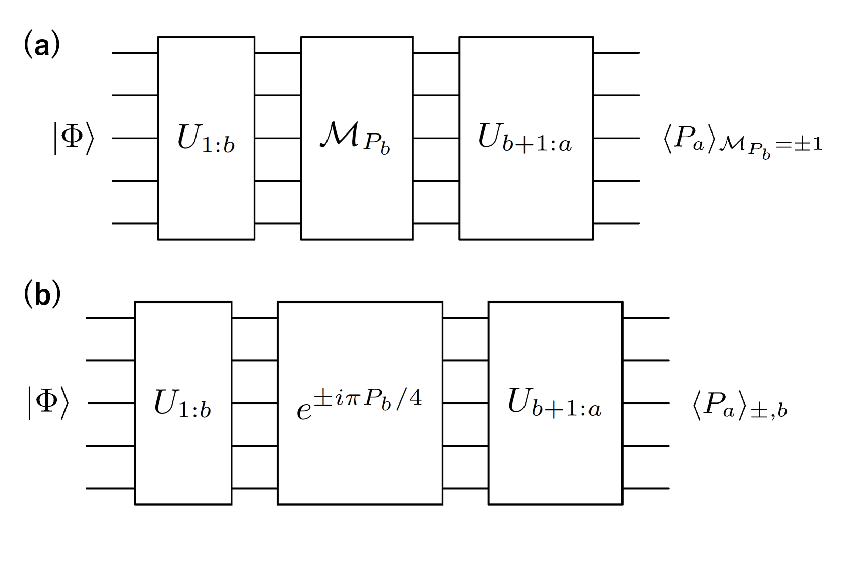
Figure 1: (a) Quantum circuit to evaluate Eq. (21) and (b) quantum circuit to evaluate Eq. (24). These figures are based on Ref. Mitarai and Fujii (2019). $\mathcal{M}_{P_{b}}$ is a projective measurement of the Pauli operator $P_{b}$.

IV.2.1 Evaluation of $\braket{\varphi_{k}}{\partial_{a}\partial_{b}\varphi_{l}}$

To calculate $\braket{\varphi_{k}}{\partial_{a}\partial_{b}\varphi_{l}}$, let us first consider evaluating

$$\bra{\Phi}U^{\dagger}(\vec{\theta})\frac{\partial}{\partial\theta_{a}}\frac{\partial}{\partial\theta_{b}}U(\vec{\theta})\ket{\Phi}$$ (19)

with $\ket{\Phi}$ being an arbitrary reference state. When $a=b$, it follows $\bra{\Phi}U^{\dagger}(\vec{\theta})\frac{\partial^{2}}{\partial\theta_{a}^{2}}U(\vec{\theta})\ket{\Phi}=-g_{a}^{2}\bra{\Phi}U^{\dagger}(\vec{\theta})U(\vec{\theta})\ket{\Phi}=-g_{a}^{2}$. When $a\neq b$, we assume $1\leq b<a\leq N_{\theta}$ without loss of generality. By using the method in Ref. Mitarai and Fujii (2019), the real and imaginary parts of Eq. (19) are evaluated separately in the following way.

The real part is calculated with quantum circuits containing projective measurements of the Pauli operator $P_{b}$ denoted by $\mathcal{M}_{P_{b}}$,

$$\begin{split}&\mathrm{Re}\left(\bra{\Phi}U^{\dagger}(\vec{\theta})\frac{\partial}{\partial\theta_{a}}\frac{\partial}{\partial\theta_{b}}U(\vec{\theta})\ket{\Phi}\right)\\ &=-g_{a}g_{b}\times\\ &\left(p(\mathcal{M}_{P_{b}}=1)\braket{P_{a}}_{\mathcal{M}_{P_{b}}=1}-p(\mathcal{M}_{P_{b}}=-1)\braket{P_{a}}_{\mathcal{M}_{P_{b}}=-1}\right),\end{split}$$ (20)

where

$$\begin{split}&\braket{P_{a}}_{\mathcal{M}_{P_{b}}=\pm 1}\\ &=\frac{1}{4}\frac{\bra{\Phi}U_{1:b}^{{\dagger}}(I\pm P_{b})U_{b+1:a}^{{\dagger}}P_{a}U_{b+1:a}(I\pm P_{b})U_{1:b}\ket{\Phi}}{p(\mathcal{M}_{P_{b}}=\pm 1)}\end{split}$$ (21)

is the conditional expectation value of $P_{a}$ when the projective measurement of $P_{b}$ yields $\pm 1$, and

$$p(\mathcal{M}_{P_{b}}=\pm 1)=\left|\frac{1}{2}(I\pm P_{b})U_{1:b}\ket{\Phi}\right|^{2}$$ (22)

is the probability of getting the result $\pm 1$ for the projective measurement of $P_{b}$. If $P_{b}$ is a single Pauli operator or even if $P_{b}$ is a multi-qubit Pauli operator, we expect that the projective measurement of it can be performed in near-term quantum devices . The total circuit for evaluating Eq. (21) is shown in Fig. 1(a).

On the other hand, the imaginary part of Eq. (19) can be calculated as

$$\begin{split}\mathrm{Im}&\left(\bra{\Phi}U^{\dagger}(\vec{\theta})\frac{\partial}{\partial\theta_{a}}\frac{\partial}{\partial\theta_{b}}U(\vec{\theta})\ket{\Phi}\right)\\ &=\frac{g_{a}g_{b}}{2}(\braket{P_{a}}_{+,b}-\braket{P_{a}}_{-,b}),\end{split}$$ (23)

where

$$\braket{P_{a}}_{\pm,b}$$ (24)

$$= \bra{\Phi}U_{1:b}^{{\dagger}}e^{\mp i\pi P_{b}/4}U_{b+1:a}^{{\dagger}}P_{a}U_{b+1:a}e^{\pm i\pi P_{b}/4}U_{1:b}\ket{\Phi},$$

is the expectation value of $P_{a}$ for the quantum state $U_{b+1:a}e^{\pm i\pi P_{b}/4}U_{1:b}\ket{\Phi}$. The circuit for calculation is shown in Fig 1(b).

Then, to obtain $\braket{\varphi_{k}}{\partial_{a}\partial_{b}\varphi_{l}}$ we take advantage of the following equality

$$\begin{split}2\braket{\varphi_{k}}{\partial_{a}\partial_{b}\varphi_{l}}=&\braket{\varphi_{k,l}^{+}}{\partial_{a}\partial_{b}\varphi_{k,l}^{+}}-\braket{\varphi_{k,l}^{-}}{\partial_{a}\partial_{b}\varphi_{k,l}^{-}}\\ &+\frac{1}{i}\left(\braket{\varphi_{k,l}^{i+}}{\partial_{a}\partial_{b}\varphi_{k,l}^{i+}}-\braket{\varphi_{k,l}^{i-}}{\partial_{a}\partial_{b}\varphi_{k,l}^{i-}}\right),\end{split}$$ (25)

where $\ket{\varphi_{k,l}^{\pm}}=U_{1:N}(\ket{\psi_{k}}\pm\ket{\psi_{l}})/\sqrt{2}$ and $\ket{\varphi_{k,l}^{i\pm}}=U_{1:N}(\ket{\psi_{k}}\pm i\ket{\psi_{l}})/\sqrt{2}$. All terms in the right hand side of (25) can be evaluated by the method described above with taking $\ket{\Phi}$ appropriately, so the $\braket{\varphi_{k}}{\partial_{a}\partial_{b}\varphi_{l}}$ is also obtained.

IV.2.2 Evaluation of $\braket{\varphi_{k}}{\partial_{c}\varphi_{l}}$

Next, we describe how to compute $\braket{\varphi_{k}}{\partial_{c}\varphi_{l}}$. It follows that

$$\begin{split}\braket{\varphi_{k}}{\partial_{c}\varphi_{l}}&=\bra{\psi_{k}}U^{\dagger}(\vec{\theta})\frac{\partial}{\partial\theta_{c}}U(\vec{\theta})\ket{\psi_{l}}\\ &=ig_{c}\bra{\psi_{k}}U^{\dagger}_{1:c}P_{c}U_{1:c}\ket{\psi_{l}}.\end{split}$$ (26)

The term in the last line can be evaluated by the method of Eq. (13) by substituting $\ket{\varphi_{k,l}^{\pm}(\vec{R})}$ by $U_{1:c}\frac{1}{\sqrt{2}}(\ket{\psi_{k}}\pm\ket{\psi_{l}})$ and $\ket{\varphi_{k,l}^{\pm i}(\vec{R})}$ with $U_{1:c}\frac{1}{\sqrt{2}}(\ket{\psi_{k}}\pm i\ket{\psi_{l}})$.

IV.2.3 Summary

In summary, calculation of the 2-NAC $D_{kl}^{I}$ proceeds as follows:

1. Perform the SSVQE or the MCVQE and obtain approximate eigenstates $\ket{\varphi_{i}(\vec{R})}$ and eigenenergies $\tilde{E}_{i}(\vec{R})$ of $H(\vec{R})$.

2. Calculate the derivative of the Hamiltonian $\frac{\partial H}{\partial R_{I}}$ on classical computers and obtain $\frac{\partial\theta^{*}_{a}}{\partial R_{I}}$ and $\frac{\partial^{2}\theta^{*}_{c}}{\partial R_{I}^{2}}$ in Eq. (18) by solving Eq. (14) and Eq. (15).

3. For all $a,b=1,\ldots,N_{\theta}$, evaluate Eq. (19) for $\ket{\Phi}=\ket{\varphi_{k,l}^{\pm}},\ket{\varphi_{k,l}^{i\pm}}$, by using Eq. (20) and Eq. (23). Plugging them in Eq. (25) yields the value of $\braket{\varphi_{k}}{\partial_{a}\partial_{b}\varphi_{l}}$.

4. For all $c=1,\ldots,N_{\theta}$, evaluate $\braket{\varphi_{k}}{\partial_{c}\varphi_{l}}$ according to Eq. (26).

5. Substituting all values obtained in previous steps into Eq. (18) gives the 2-NAC.

The main contribution of this paper is that we reduce the definition of the NACs (Eqs. (1) and (2)) to the formulas that we can evaluate on quantum devices by the existing techniques. Here we note that the procedure 2 follows the techniques in Ref. Mitarai et al. (2020), the procedure 3 partially uses those in Ref. Mitarai and Fujii (2019), and the procedure 4 basically follows those in Ref. Nakanishi et al. (2019).

V Calculating Berry’s phase with variational quantum eigensolver

In this section, we describe a method for calculating Berry’s phase with the VQE algorithm. From the results of the VQE, while we can access the density operators of the eigenstate $\rho_{k}(\vec{\theta}^{*})=\ket{\varphi_{0}(\vec{\theta}^{*})}\bra{\varphi_{0}(\vec{\theta}^{*})}$ determined by the optimized circuit-parameters $\vec{\theta}^{*}$, we cannot access the information about the phase of quantum state. Here we discuss how to calculate Berry’s phase on quantum devices from the optimized circuit-parameters obtained by the VQE. In the following, without loss of generality, we only consider the ground state as the eigenstate. Let $\mathcal{N}_{0}$ denote the set of normalized states in a complex Hilbert space $\mathcal{H}$. We consider performing the VQE from one point $\vec{R}_{0}\coloneqq\vec{R}(t_{0})$ of the closed loop $\mathcal{C}_{\vec{R}}\coloneqq\{\vec{R}(t)\mid t\in[t_{0},t_{1}],\vec{R}(t_{0})=\vec{R}(t_{1})\}$ in the system-parameters space and continue doing it along $\mathcal{C}_{\vec{R}}$, then we obtain a smooth curve $\mathcal{C}_{\vec{\theta}^{*}}\coloneqq\{\vec{\theta}^{*}(\vec{R}(t))\mid t\in[t_{0},t_{1}]\}$ in the circuit-parameter space. For simplicity, let $\vec{\theta}^{*}_{\mathrm{s}}\coloneqq\vec{\theta}^{*}(\vec{R}(t_{0}))$ and $\vec{\theta}^{*}_{\mathrm{t}}\coloneqq\vec{\theta}^{*}(\vec{R}(t_{1}))$ denote the starting point and the end point of $\mathcal{C}_{\vec{\theta}^{*}}$, respectively. We note that $\vec{\theta}^{*}_{\mathrm{s}}\neq\vec{\theta}^{*}_{\mathrm{t}}$ may occur, i.e., the curve $\mathcal{C}_{\vec{\theta}^{*}}$ of the optimal parameters does not necessarily form the closed loop in the circuit-parameter space even when $\mathcal{C}_{\vec{R}}$ is the closed loop in the system-parameter space. This is because the VQE does not care about the overall phase of the ground state, and for most cases there is a redundancy in the ansatz $\ket{\varphi_{0}(\vec{\theta})}$ such that $\ket{\varphi_{0}(\vec{\theta}_{1})}=e^{i\xi}\ket{\varphi_{0}(\vec{\theta}_{2})},e^{i\xi}\neq 1$ for some $\vec{\theta}_{1}\neq\vec{\theta}_{2}$. Next, we introduce the projective Hilbert space called Ray space. Ray space $\mathcal{R}$ is defined as the equivalent class $\mathcal{R}\coloneqq\mathcal{N}_{0}/\sim$ where the equivalence relation $\sim$ holds for two elements of $\mathcal{N}_{0}$ which differ only by a global phase. We also define the projection map $\pi:\ket{\psi}\in\mathcal{N}_{0}\rightarrow\rho=\ket{\psi}\bra{\psi}\in\mathcal{R}$. For a given curve $\mathcal{C}_{\mathcal{N}_{0}}=\{\ket{\varphi_{0}(\vec{\theta}^{*})}\}\subset\mathcal{N}_{0}$, its projection to $\mathcal{R}$ is also the curve $\mathcal{C}_{\rho}\coloneqq\{\rho(\vec{\theta}^{*})\mid\rho=\ket{\varphi_{0}(\vec{\theta}^{*})}\bra{\varphi_{0}(\vec{\theta}^{*})},\vec{\theta}^{*}\in\mathcal{C}_{\vec{\theta}^{*}}\}\subset\mathcal{R}$, and this curve $\mathcal{C}_{\rho}$ in $\mathcal{R}$ is determined uniquely according to the optimized circuit-parameters $\vec{\theta}^{*}$.

Then let us describe and formulate the way to calculate Berry’s phase based on the results of the VQE. Suppose that a curve $\mathcal{C}_{\rho}=\{\rho(\vec{\theta}^{*})\}$ is given. Here, we consider a particular lift $\mathcal{C}_{\mathcal{N}_{0}}=\{\ket{\varphi_{0}(\vec{\theta}^{*})}\}$ of $\mathcal{C}_{\rho}$ such that $\pi(\mathcal{C}_{\mathcal{N}_{0}})=\mathcal{C}_{\rho}$ where $\ket{\varphi_{0}(\vec{\theta}^{*})}$ is fixed up to a phase. We assume that $\ket{\varphi_{0}(\vec{\theta}^{*})}$ is smooth, i.e., $\ket{\varphi_{0}(\vec{\theta}^{*})}$ is differentiable with respect to $\vec{\theta}^{*}$. With this lift $\mathcal{C}_{\mathcal{N}_{0}}$, Berry’s phase can be defined as Mukunda and Simon (1993)

$$\begin{split}\Pi_{\mathcal{C}_{\rho}}\coloneqq-i\int_{\vec{\theta}^{*}_{\mathrm{s}}}^{\vec{\theta}^{*}_{\mathrm{t}}}d\vec{\theta}^{*}\cdot&\braket{\varphi_{0}(\vec{\theta}^{*})}{\frac{\partial}{\partial\vec{\theta}^{*}}}{\varphi_{0}(\vec{\theta}^{*})}\\ &\quad\quad\quad\quad\quad+\arg(\braket{\varphi_{0}(\vec{\theta}^{*}_{\mathrm{s}})}{\varphi_{0}(\vec{\theta}^{*}_{\mathrm{t}})}).\end{split}$$ (27)

We want to emphasize here that Berry’s phase is a functional of the curve $\mathcal{C}_{\rho}$. Namely, for a given curve $\mathcal{C}_{\rho}$, though we can construct a new curve $C^{\prime}_{\mathcal{N}_{0}}$ which differs only by $U(1)$ phase degree of freedom from $\mathcal{C}_{\mathcal{N}_{0}}$ with a real smooth function $\Theta(\vec{\theta}^{*})$,

$$\begin{split}\mathcal{C}_{\mathcal{N}_{0}}\rightarrow C^{\prime}_{\mathcal{N}_{0}}:\quad&\ket{\varphi_{0}^{\prime}(\vec{\theta}^{*})}=e^{i\Theta(\vec{\theta}^{*})}\ket{\varphi_{0}(\vec{\theta}^{*})},\\ \pi(\mathcal{C}_{\mathcal{N}_{0}})&=\pi(C^{\prime}_{\mathcal{N}_{0}}),\end{split}$$ (28)

the value of Berry’s phase $\Pi_{\mathcal{C}_{\rho}}$ calculated with the curve $\mathcal{C}^{\prime}_{\mathcal{N}_{0}}$ is identical to that with $\mathcal{C}_{\mathcal{N}_{0}}$.

As discussed above, by performing the VQE, we obtain the curves $\mathcal{C}_{\vec{\theta}^{*}}$ and $\mathcal{C}_{\rho}$. To calculate Berry’s phase based on the Eq. (27), we have to choose some fixed lift $\mathcal{C}_{\mathcal{N}_{0}}$ from $\mathcal{C}_{\mathcal{\rho}}$. Due to the arbitrariness of the lift, we can fix the phase freedom globally and choose $\mathcal{C}_{\mathcal{N}_{0}}$ so that the freedom does not depend on $\vec{\theta}^{*}$. Therefore, given a $\rho(\vec{\theta}^{*}_{\mathrm{s}})$, we first choose $\ket{\varphi_{0}(\vec{\theta}^{*}_{\mathrm{s}})}$ up to phase, and then form a lift $\mathcal{C}_{\mathcal{N}_{0}}=\{\ket{\varphi_{0}(\vec{\theta}^{*})}\}$ uniquely up to a phase degree of freedom in the starting point of the curve $\ket{\varphi_{0}(\vec{\theta}^{*}_{\mathrm{s}})}$. By considering such lift, the terms appearing in the Eq. (27) can be reduced to the quantities which can be evaluated with quantum devices. In the following, we explain how to evaluate the terms in the right hand side of Eq. (27).

V.1 Evaluation of the first term

The first term of Eq. (27) is computed by discretization of the closed loop $\mathcal{C}_{\vec{R}}$ and numerical integration of the integrand. We discretize the value of the system-parameters $\vec{R}$ on $\mathcal{C}_{\vec{R}}$ as $\vec{R}_{0},\ldots,\vec{R}_{K-1}$ appropriately and also define $\vec{R}_{K}=\vec{R}_{0}$. The VQE algorithm is performed for all points $\{\vec{R}_{p}\}_{p=0}^{K}$ and the optimal circuit-parameters are obtained as $\{\vec{\theta}^{*}_{p}=\vec{\theta}^{*}(\vec{R}_{p})\}_{p=0}^{K}$. We define $\vec{\theta}_{0}^{*}\coloneqq\vec{\theta}^{*}_{\mathrm{s}}(\vec{R}_{0})$ and $\vec{\theta}_{K}^{*}\coloneqq\vec{\theta}^{*}_{\mathrm{t}}(\vec{R}_{0})$ and stress again that $\vec{\theta}_{0}^{*}\neq\vec{\theta}_{K}^{*}$ may hold in general due to the redundancy of the ansatz. Here because we choose the phase freedom of the lift $\mathcal{C}_{\mathcal{N}_{0}}=\{\ket{\varphi_{0}(\vec{\theta}^{*})}\}$ which is independent on $\vec{\theta}^{*}$, the integrand of the first term can be written as

$$\begin{split}\braket{\varphi_{0}(\vec{\theta}^{*})}{\frac{\partial}{\partial\theta_{a}^{*}}}{\varphi_{0}(\vec{\theta}^{*})}&=\bra{\psi_{0}}U^{\dagger}(\vec{\theta}^{*})\frac{\partial}{\partial\theta_{a}^{*}}U(\vec{\theta}^{*})\ket{\psi_{0}}\\ &=ig_{a}\bra{\psi_{0}}U^{*{\dagger}}_{1:a}P_{a}U_{1:a}^{*}\ket{\psi_{0}},\end{split}$$ (29)

so it is evaluated by measuring the expectation value of $P_{a}$ for the state $U_{1:a}^{*}\ket{\psi_{0}}$, which can be evaluated on quantum devices. Therefore the integral is approximated by

$$\int_{\mathcal{C^{\prime}}}d\vec{\theta}^{*}\cdot\braket{\varphi_{0}(\vec{\theta}^{*})}{\frac{\partial}{\partial\vec{\theta}^{*}}}{\varphi_{0}(\vec{\theta}^{*})}$$ (30)

$$\approx \sum_{p=0}^{K-1}(\vec{\theta}_{p+1}^{*}-\vec{\theta}_{p}^{*})\cdot\left.\braket{\varphi_{0}(\vec{\theta}^{*})}{\frac{\partial}{\partial\vec{\theta}^{*}}}{\varphi_{0}(\vec{\theta}^{*})}\right|_{\vec{\theta}^{*}=\vec{\theta}^{*}_{p}}.$$

V.2 Evaluation of the second term

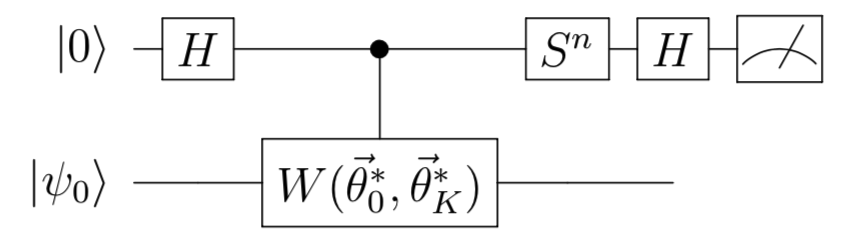
Figure 2: The Hadamard test to evaluate the phase difference $\arg(\braket{\varphi(\vec{\theta}^{*}_{\mathrm{s}})}{\varphi(\vec{\theta}^{*}_{\mathrm{t}})})$ in Eq. (27). The upper line represents an ancillary qubit which is measured, and the lower line represents the system on which $W(\vec{\theta}_{0}^{*},\vec{\theta}_{K}^{*})\coloneqq U^{{\dagger}}(\vec{\theta}^{*}_{K})U(\vec{\theta}^{*}_{0})$ operates. The results of the measurements for the ancillary qubit gives the value of $\mathrm{Re}\left(\braket{\varphi(\vec{\theta}_{0}^{*})}{\varphi(\vec{\theta}_{K}^{*})}\right)$ and $\mathrm{Im}\left(\braket{\varphi(\vec{\theta}_{0}^{*})}{\varphi(\vec{\theta}_{K}^{*})}\right)$ for $n=0,1$.

The second term in Eq. (27), $\arg(\braket{\varphi_{0}(\vec{\theta}^{*}_{\mathrm{s}})}{\varphi_{0}(\vec{\theta}^{*}_{\mathrm{t}})})$, is evaluated by the difference of the overall phase of two wavefunctions $\ket{\varphi_{0}(\theta^{*}_{0})}$ and $\ket{\varphi_{0}(\theta^{*}_{K})}$. This can be performed by estimating $\arg(\braket{\varphi_{0}(\theta^{*}_{0})}{\varphi_{0}(\theta^{*}_{K})})=\arg(\braket{\psi_{0}}{U^{{\dagger}}(\vec{\theta}^{*}_{0})U(\vec{\theta}^{*}_{K})}{\psi_{0}})$ with the Hadamard test Cleve et al. (1998) depicted in Fig. 2. It requires one ancillary qubit and the controlled-$U(\vec{\theta})$ gates, which are costly for near-term quantum devices. We finally mention that if we construct the lift $\mathcal{C}_{\mathcal{N}_{0}}$ of $\mathcal{C}_{\rho}$ so that the phase degree of freedom depends on $\vec{\theta}^{*}$, by taking both terms in Eq. (27) into account, Eq. (27) can be reduced to the quantities which can be evaluated on quantum devices as discussed above .

V.3 Comparison with previous studies

We here compare previous work on calculating Berry’s phase on quantum devices with our method. In Ref. Murta et al. (2020), Berry’s phase is calculated by simulating adiabatic dynamics of the system $U_{\mathcal{C}}=\mathcal{T}e^{-i\int_{0}^{T}dsH(s)}$, where $\mathcal{T}$ is the time-ordered product and $H(s)$ is a time-dependent Hamiltonian, which varies along the closed loop $\mathcal{C}$ in sufficiently long time $T$. $U_{\mathcal{C}}$ is implemented on quantum computers by the Suzuki-Trotter decomposition, and the Hadamard test like Fig. 2 is performed to detect the phase difference between the initial ground state $\ket{\chi(\vec{R}_{0})}$ and the time-evolved state $U_{\mathcal{C}}\ket{\chi(\vec{R_{0}})}$. The phase difference between $\ket{\chi(\vec{R}_{0})}$ and $U_{\mathcal{C}}\ket{\chi(\vec{R_{0}})}$ contains the dynamical phase and Berry’s phase, but the former phase can be neglected by combining the forward- and backward-time evolutions by assuming the Hamiltonian of the system has the time-reversal symmetry. Compared with this strategy, our proposal for calculating Berry’s phase based on the VQE has two features. First, we do not have to assume the time-reversal symmetry in the system to remove the contribution from the dynamical phase like in the previous study because we directly calculate Berry’s phase based on the definition Eq. (6). Our method can apply to general quantum systems. Second, the causes of errors are quite different. More concretely, while the errors in the previous methods arise from the Trotterization of the time evolution operator, the errors in our method mainly come from two sources: one is the approximation error of the eigenstates obtained by the VQE, and the other is the numerical error of integration in Eq. (30). These errors can be reduced by deepening the ansatz circuits and taking more discretized points on $\mathcal{C}$, respectively. We comment that further research is needed to conclude the difference in the performance between our method and these previous methods.

Finally, we introduce another method to calculate Berry’s phase based on the VQE with a lot of Hadamard tests. Using the formula

$$\Pi_{\mathcal{C}}\approx-i\sum_{i=0}^{K}\mathrm{Im}\left(\ln\braket{\varphi_{0}(\vec{\theta}^{*}_{i})}{\varphi_{0}(\vec{\theta}^{*}_{i+1})}\right),$$ (31)

with taking the principal branch of the complex logarithm, $-\pi\leq\mathrm{Im}(z)<\pi$ for $z\in\mathbb{C}$, is one of the candidates for avoiding discretization error of the closed loop $\mathcal{C}$ and numerical instability Fukui et al. (2005). The value of $\braket{\varphi_{0}(\vec{\theta}^{*}_{i})}{\varphi_{0}(\vec{\theta}^{*}_{i+1})}$ is evaluated by the Hadamard test in Fig. 2 by substituting $\vec{\theta}_{0(K)}^{*}$ with $\vec{\theta}_{i(i+1)}^{*}$.

V.4 Summary

Berry’s phase can be calculated based on the VQE as follows:

1. Discretize the closed loop $\mathcal{C}$ in the system-parameters space as $\{\vec{R}_{p}\}_{p=0}^{K}$ appropriately and perform the VQE for all points.

2. Calculate the first term of Eq. (27) by using Eq. (29) and Eq. (30).

3. If necessary, evaluate the phase difference $\arg(\braket{\varphi_{0}(\vec{\theta}^{*}_{\mathrm{s}})}{\varphi_{0}(\vec{\theta}^{*}_{\mathrm{t}})})$ by the Hadamard test shown in Fig. 2.

4. Substituting all values obtained in the previous steps into Eq. (27) gives the Berry’s phase.

VI Experiment on a real quantum device

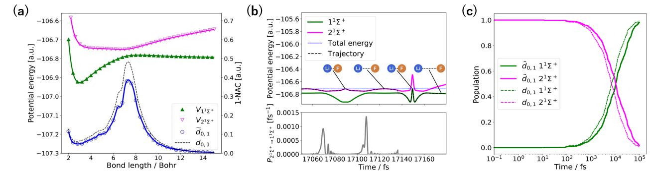
Figure 3: (a) Numerical results of the potential energy curves of the $1^{1}\Sigma^{+}$ state (upper triangles) and $2^{1}\Sigma^{+}$ state (lower triangles) of LiF obtained by the SSVQE and experimental results of the 1-NAC $\tilde{d}_{0,1}$ between the two states (circles) at the bond distance $R$ in the range of $2$ to $15$ Bohr. The solid lines represent the spline interpolated curves computed by SciPy, a numerical library in Python Virtanen et al. (2020). The dashed lines show the exact numerical results of the 1-NAC $d_{0,1}$ in a noiseless situation calculated with the Qiskit’s statevector simulator Qis (2020). The exact potential energy curves calculated by the exact diagonalization are not presented in the figure since they coincide with the ones obtained by the SSVQE (presented in the figure) by less than $10^{-10}$ a.u. for the whole range of $R$. (b) Potential energies of $1^{1}\Sigma^{+}$ state and $2^{1}\Sigma^{+}$ state (upper panel) of LiF and the transition probability $P_{2^{1}\Sigma^{+}\rightarrow 1^{1}\Sigma^{+}}$ (lower panel) for one trajectory obtained by the TSH molecular dynamics simulation using $\tilde{d}_{0,1}$ values in (a). On this trajectory, the molecule hops from $2^{1}\Sigma^{+}$ state to $1^{1}\Sigma^{+}$ state at 17136.2 fs during bond shrinking motion and it is dissociated into Li and F atoms. (c) Time evolution of the population of the $1^{1}\Sigma^{+}$ state and $2^{1}\Sigma^{+}$ state of LiF computed by 500 trajectories of TSH simulation using the values of 1-NAC, $\tilde{d}_{0,1}$ and $d_{0,1}$, in (a).

In this section, we show an experimental result of our algorithm for the 1-NAC on a real quantum device and the non-adiabatic molecular dynamics (MD) simulation based on the experimental values of the 1-NAC.

We consider a lithium fluoride (LiF) molecule with bond length $R$ and its electronic states under the Born-Oppenheimer approximation. In this system, the potential energy curves, or eigenenergies $E$ as a function of $R$, of the two lowest ${}^{1}\Sigma^{+}$ states are known to exhibit the avoided crossing Werner and Meyer (1981); Bauschlicher and Langhoff (1988); Bandrauk and Gauthier (1989, 1990), and it plays a crucial role for nonadiabatic dynamics such as photodissociation. Here we focus on this avoided crossing and the resulting nonadiabaitc dynamics by modeling the system with a simple two-state model. Specifically, the electronic Hamiltonian of LiF at bond distance $R$ is constructed by two orbitals obtained by the state-average complete active space self-consistent field (CASSCF) method Sun et al. (2017). By considering symmetries in the system, one can obtain a two-qubit Hamiltonian $H_{\mathrm{LiF}}(R)$ from that electronic Hamiltonian. Further details are described in Appendix A.

We run our algorithm to calculate the 1-NAC (Sec. IV) of $H_{\mathrm{LiF}}(R)$ at various bond length $R$ in the IBM Q cloud quantum device (ibmq_valencia) IBM (2020). First, the SSVQE calculation for $H_{\mathrm{LiF}}(R)$ is performed on a classical simulator where the exact and noiseless expectation values of observables are obtained. The ansatz for the SSVQE, $U(\vec{\theta})$, is depicted in Fig. 4

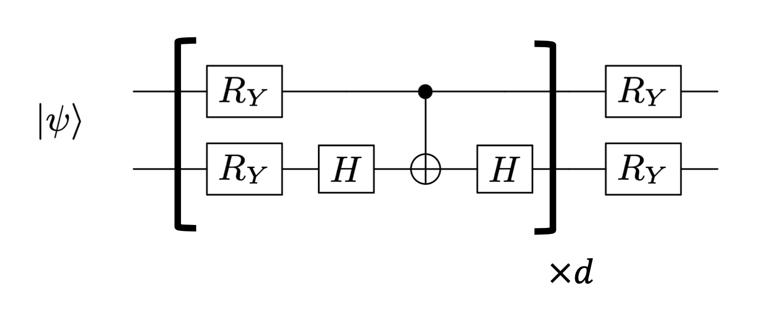
Figure 4: The ansatz circuit $U(\vec{\theta})$ for the SSVQE. Each $R_{Y}=\exp(-iY\theta/2)=\begin{pmatrix}\cos\theta/2&\sin\theta/2\\ -\sin\theta/2&\cos\theta/2\\ \end{pmatrix}$ has a rotational angle $\theta$ as an independent parameter, and $d=4$ denotes the depth of the ansatz. The rotation angles of $R_{Y}$ gates are optimized during the SSVQE in our experiments. We note that quantum states generated by this circuit for real wavefunction $\ket{\psi}$ remain real for any choice of $\theta$.

and we optimize the parameters $\vec{\theta}$ to minimize the cost function (10). The initial states to which the ansatz applied are $\ket{\psi_{0}}=\ket{00},\ket{\psi_{1}}=\ket{01}$ states. To calculate the singlet ($S=0$) states ${}^{1}\Sigma^{+}$, we penalize the triplet ($S=1$) states by modifying the Hamiltonian in the cost function as $H^{\prime}=H_{\mathrm{LiF}}(R)+\beta\hat{S}^{2}$, where $\hat{S}^{2}$ is the spin squared operator and $\beta=4.0$ is a constant Kuroiwa and Nakagawa (2021). We obtain the (approximate) eigenstates $\ket{\varphi_{0,1}(\vec{\theta}^{*})}=U(\vec{\theta}^{*})\ket{\psi_{0,1}}$ and eigenenergies $\tilde{E}_{0,1}$ for two ${}^{1}\Sigma^{+}$ states in this way from the classical simulator (Fig. 3(a) shows the potential energy curves). Next, the transition amplitude $\braket{\varphi_{0}(\vec{\theta}^{*})}{\frac{dH_{\mathrm{LiF}}(R)}{dR}}{\varphi_{1}(\vec{\theta}^{*})}$ is computed on a quantum device by evaluating each term of the right hand sides of Eq. (13) with 8192 shots. Since the wavefunction is real by definition of the ansatz $U(\vec{\theta})$, we consider only the real part of Eq. (13). Finally, the 1-NAC is obtained by plugging the estimate of $\braket{\varphi_{0}(\vec{\theta}^{*})}{\frac{dH_{\mathrm{LiF}}(R)}{dR}}{\varphi_{1}(\vec{\theta}^{*})}$ into the numerator of Eq. (3) and that of $\tilde{E}_{0}-\tilde{E}_{1}$ into the denominator. As we mentioned in Sec. II, the 1-NAC is not gauge invariant. Even when considering only real wavefunctions as in this case, the 1-NAC still has indefinite sign, but here the sign is determined by considering the continuity of the 1-NAC with respect to the nuclear coordinate $\vec{R}$. We comment that the way of calculating the 1-NAC here is chosen to remove the effect of the noise and errors in the real quantum device during the SSVQE and focus on evaluating the transition amplitude.

The result of the 1-NAC is shown in Fig. 3(a). Because of the noise in the real quantum device, the values of the transition amplitude are smaller than the exact results but still qualitatively consistent with them. This shrinking could be resolved by, for example, using the error mitigation technique Temme et al. (2017); Endo et al. (2018) for near-term quantum devices.

In addition, we perform the trajectory surface hopping (TSH) Tully and Preston (1971) molecular dynamics calculation using Tully’s fewest switches algorithm Tully (1990) based on the obtained values of the potential energy curves and the 1-NAC (Fig. 3(a)). We assume a situation where a LiF molecule is excited by light to the first electronic excited state. In the TSH simulation, the nuclear energy gradient $\frac{\partial\tilde{E}_{0,1}}{\partial R}$ and the 1-NAC at various bond lengths $R$ are requested by the TSH program code, and we feed it with the values interpolated from the results of the SSVQE and the 1-NAC experiment. The details of the interpolation are described in Appendix B. We prepare a set of 500 molecular geometries and nuclear velocities as a harmonic-oscillator Wigner distribution for the vibrational ground state at the equilibrium geometrical structure in the electronic ground state $1^{1}\Sigma^{+}$. We run the trajectories from the first electronic excited state $2^{1}\Sigma^{+}$ with a time step of 0.1 fs and find that the trajectories hop from $2^{1}\Sigma^{+}$ to $1^{1}\Sigma^{+}$ where the dissociation occurs as shown in Fig. 3(b). The dynamics of the populations of the $1^{1}\Sigma^{+}$ state and $2^{1}\Sigma^{+}$ state is calculated based on the results of 500 trajectories and shown in Fig. 3(c). Since the experimentally-obtained 1-NAC values are smaller than the noiseless simulation ones (Fig. 3(a)), the decay of the $2^{1}\Sigma^{+}$ population calculated by using the experimental values of 1-NAC is slightly slower than that is calculated by using the noiseless simulation values of 1-NAC. Nevertheless, the overall dynamics of the populations is similar to each other and this indicates the possibility of performing TSH in a quantum device in the near future.

The TSH simulation is conducted by the open-source library SHARC Mai et al. (2019); Richter et al. (2011); Mai et al. (2018).

Although we consider the 1-NAC throughout this section, we perform additional numerical demonstrations of our methods by simulating the quantum circuits to calculate the 1-NAC and 2-NAC of the hydrogen molecules and Berry’s phase of a two-site spin model in Appendix D.

VII Discussion

Our proposed methods presented in the previous sections are based on the analytical derivative of the eigenstates obtained by the SSVQE. This section compares our methods with those using the numerical derivative of the eigenstates by the finite difference method. The comparison will be made from two points of view: (1) the number of distinct Hamiltonians to perform the SSVQE to obtain the optimal circuit-parameters $\vec{\theta}^{*}$ and (2) the total number of measurements required to evaluate the NACs and Berry’s phase after performing the SSVQE. We ignore the cost of classical computation throughout analyses in this section.

We recall that $N_{\theta}$ and $N_{x}$ are the dimensions of the circuit-parameters and system-parameters, respectively. The number of qubits in the system is denoted as $n$ and the number of Pauli terms in the Hamiltonian as $N_{H}$. For quantum chemistry problems $N_{H}$ is typically $O(n^{4})$ McArdle et al. (2020); Cao et al. (2019), but several methods for reducing $N_{H}$ are proposed Motta et al. (2018); Huggins et al. (2021). The detailed derivations of the formulas in this section (Eqs. (32), (34), and (37)) are presented in Appendix C.

VII.1 Cost of 1-NAC

Let us consider our proposed method to calculate the 1-NAC $d_{kl}^{I}$ with fixed $k,l$ and all $I=1,\ldots N_{x}$ at some fixed system-parameters $\vec{R}$. The evaluation of the 1-NAC is performed by calculating the denominator and numerator in Eq. (3). Both can be obtained by applying a single optimized ansatz circuit $U(\vec{\theta}^{*}(\vec{R}))$ resulting from the SSVQE to several initial states and measuring appropriate observables, so the number of distinct Hamiltonians to perform the SSVQE is just one. Meanwhile, the number of measurements to calculate the 1-NAC is estimated as follows. When we write the Hamiltonian as $H(\vec{R})=\sum_{i=1}^{N_{H}}h_{i}(\vec{R})P_{i}$, where $P_{i}$ is Pauli operator and $h_{i}(\vec{R})$ is a real coefficient, the values of $\braket{\varphi_{k(l)}}{H(\vec{R})}{\varphi_{k(l)}}=\sum_{i=1}^{N_{H}}h_{i}(\vec{R})\braket{\varphi_{k(l)}}{P_{i}}{\varphi_{k(l)}}$ and $\braket{\varphi_{k}}{\partial H(\vec{R})/\partial R_{I}}{\varphi_{l}}=\sum_{i=1}^{N_{H}}\partial h_{i}(\vec{R})/\partial R_{I}\braket{\varphi_{k}}{P_{i}}{\varphi_{l}}$ are necessary to compute the 1-NAC. The term $\braket{\varphi_{k(l)}}{P_{i}}{\varphi_{k(l)}}$ is evaluated as the expectation value of $P_{i}$, and similarly the term $\braket{\varphi_{k}}{P_{i}}{\varphi_{l}}$ ($i=1,\ldots,N_{H}$) is evaluated as a sum of four expectation values in the right hand sides of Eq. (13). By taking into account errors in evaluating those expectations values, the number of measurements to estimate the 1-NAC within the error $\epsilon$ is given by

$$\begin{split}&N_{\mathrm{total}}^{\mathrm{1\mathchar 45\relax NAC}}\\ &=O\left[\frac{N_{H}}{\epsilon^{2}|\Delta E_{k,l}|^{4}}\left(|\Delta E_{k,l}|\left\|\frac{\partial H}{\partial R_{I^{*}}}\right\|+\|H\||A_{I^{*}}|\right)^{2}\right],\end{split}$$ (32)

where $A_{I}(\Delta E_{k,l})$ is the numerator (denominator) of Eq. (3), $\|H\|=\sum_{i}|h_{i}|$, $\|\partial H/\partial R_{I}\|=\sum_{i}|\partial h_{i}/\partial R_{I}|$, and $I^{*}=\mathrm{argmax}_{I}\left(|\Delta E_{k,l}|\left\|\frac{\partial H}{\partial R_{I}}\right\|+\|H\||A_{I}|\right)$. It scales with the number of the Pauli terms in the Hamiltonian but does not depend on the number of circuit-parameters $N_{\theta}$ by virtue of Eq. (3). The dependence on $I$, or the system-parameters, is also absent because it is absorbed into the classical computation of the coefficient $\partial h_{i}(\vec{R})/\partial R_{I}$ Mitarai et al. (2020).

To compare with our method, one can consider a method to evaluate the 1-NAC based on numerical differentiation of the eigenstates obtained by the SSVQE. In such approach, the 1-NAC can be evaluated by the following formula,

$$d_{k,l}^{I}\approx\frac{\tau_{k,l}(\vec{R},\vec{R}+h\vec{e}_{I})-\tau_{k,l}(\vec{R},\vec{R}-h\vec{e}_{I})}{2h},$$ (33)

where $\tau_{k,l}(\vec{R},\vec{R}\pm h\vec{e}_{I})$=$\braket{\varphi_{k}(\vec{\theta}^{*}(\vec{R}))}{\varphi_{l}(\vec{\theta}^{*}(\vec{R}\pm h\vec{e}_{I}))}$, $h$ is a positive number, and $\vec{e}_{I}$ is the unit vector in $I$-th direction. For simplicity, we will represent $\tau_{k,l}(\vec{R},\vec{R}\pm h\vec{e}_{I})$ as $\tau_{k,l}^{\pm,I}$.

When evaluating each term of Eq. (33), we assume that ${\tau_{k,l}^{\pm,I}}$ is estimated from the overlap $\left|\braket{\psi_{k}}{U^{{\dagger}}(\vec{\theta}^{*}(\vec{R}))U(\vec{\theta}^{*}(\vec{R}\pm h\vec{e}_{I}))}{\psi_{l}}\right|^{2}$, which can be easily evaluated from measurements on near-term quantum devices if $\ket{\psi_{k}},\ket{\psi_{l}}$ are computational basis states Higgott et al. (2019). We then obtain the value of $\tau_{k,l}^{\pm,I}$ by taking the square root of the overlaps with a positive sign (real value) Havlíček et al. (2019). This treatment can be justified when we solve problems in quantum chemistry, where wavefunctions are often real, and we adopt an ansatz which produces a real wavefunction. This approach to evaluate Eq. (33) avoids the costly Hadamard test and is considered to be feasible on near-term quantum devices. We note that our methods are always applicable without the assumption above.

To evaluate the 1-NAC with Eq. (33), we need optimal parameters $\vec{\theta}^{*}(\vec{R}),\vec{\theta}^{*}(\vec{R}\pm h\vec{e}_{I})$ for all $I$, so the number of distinct Hamiltonians to perform the SSVQE in the finite difference method is $2N_{x}+1=O(N_{x})$. By considering the error in estimating the overlaps, the number of measurements to estimate the 1-NAC with the precision of $\epsilon$ in the finite difference method is at least

$${N^{{}^{\prime}}}_{\mathrm{total}}^{\mathrm{1\mathchar 45\relax NAC}}=O(N_{x}/T_{k,l}^{2}\epsilon^{2}),$$ (34)

where $T_{k,l}=\min_{\sigma=\pm,I}\tau_{k,l}^{\sigma,I}$ and we assume the condition $M_{3}\geq O(\epsilon)$, where $M_{3}=\max_{I}\max_{s\in[-h,h]}\left|\tau_{k,l}^{(I,3)}(s)\right|$ and $\tau_{k,l}^{(I,3)}(s)=\frac{d^{3}}{ds^{3}}\tau_{k,l}(\vec{R},\vec{R}+s\vec{e}_{I})$. Both our method (32) and the finite difference method (34) scale with $\epsilon^{-2}$, so the prefactors determine the efficiency of them. When $N_{x}$, or the number of system-parameters (nuclei of the molecule), becomes large, the finite difference method will suffer from a large number of the SSVQE runs and the measurements compared with our method.

VII.2 Cost of 2-NAC

To calculate the 2-NAC $D_{kl}^{I}$ with fixed $k,l$ and all $I=1,\ldots N_{x}$ at $\vec{R}$ with our method, we require one optimized circuit-parameter $\theta^{*}(\vec{R})$, so the number of distinct Hamiltonians to perform the SSVQE is again one. Let us consider the number of measurements. We need the derivatives $\{\frac{\partial\theta^{*}_{a}}{\partial R_{I}},\frac{\partial^{2}\theta^{*}_{a}}{\partial R_{I}^{2}}\}_{I=1}^{N_{x}}$ which are obtained as the solutions of Eqs. (14)(15). The coefficients of these equations are determined within error $\epsilon$ by performing $O(N_{\theta}^{3}N_{H}/\epsilon^{2})$ measurements. Since the error propagation from the coefficients to the solutions $\{\frac{\partial\theta^{*}_{a}}{\partial R_{I}},\frac{\partial^{2}\theta^{*}_{a}}{\partial R_{I}^{2}}\}_{I=1}^{N_{x}}$ is very complicated, we here let the error of the solutions be $\epsilon$ (see Ref. Mitarai et al. (2020) for similar discussion). The value of $\braket{\varphi_{k}}{\partial_{a}\partial_{b}\varphi_{l}}(a,b=1,\ldots,N_{\theta})$ in Eq. (25) is obtained by measuring $O(N_{\theta}^{2}/\epsilon^{2})$ times within error $\epsilon$. Similarly, $\braket{\varphi_{k}}{\partial_{c}\varphi_{l}}(c=1,\ldots,N_{\theta})$ in Eq. (26) is calculated by $O(N_{\theta}/\epsilon^{2})$ measurements. Therefore, the total number of measurements to evaluate the 2-NAC by our method is roughly given by

$$N_{\mathrm{total}}^{\mathrm{2\mathchar 45\relax NAC}}=O(N_{\theta}^{3}N_{H}/\epsilon^{2}),$$ (35)

where the meaning of $\epsilon$ has to be cared for. It does not depend on the number of system-parameters $N_{x}$.

The finite difference method is based on the following formula:

$$D_{k,l}^{I}\approx\frac{\tau_{k,l}(\vec{R},\vec{R}+h\vec{e}_{I})+\tau_{k,l}(\vec{R},\vec{R}-h\vec{e}_{I})}{h^{2}}$$ (36)

where we used $\tau_{k,l}(\vec{R},\vec{R})=0$. Similarly to the case of the 1-NAC, the number of distinct Hamiltonians to perform the SSVQE is $O(N_{x})$. To bound the error of the 2-NAC by $\epsilon$, the finite difference method requires at least

$${N^{{}^{\prime}}}_{\mathrm{total}}^{\mathrm{2\mathchar 45\relax NAC}}=O\left(N_{x}^{2}/T_{k,l}^{2}\epsilon^{2}\right)$$ (37)

measurements under the condition $M_{4}\geq O(\epsilon)$, where $M_{4}=\max_{I}\max_{s\in[-h,h]}\left|\tau_{k,l}^{(I,4)}(s)\right|$ and $\tau_{k,l}^{(I,4)}(s)=\frac{d^{4}}{ds^{4}}\tau_{k,l}(\vec{R},\vec{R}+s\vec{e}_{I})$. The number of measurements in our method (35) does not depends on $N_{x}$ while the finite difference method (37) does, as with the 1-NAC.

VII.3 Cost of Berry’s phase

For calculating Berry’s phase, the closed path $\mathcal{C}$ is discretized into $K$ points. The integrand (Eq. (27)) is evaluated at all $K$ points and numerically integrated both in our method and the finite difference method. We therefore compare our method with the finite difference method only in terms of the cost to obtain the integrand at all the discretized points.

In our method, the integrand at each discretized point can be evaluated by Eq. (29). The total number of distinct Hamiltonians to perform the VQE is $K+1=O(K)$. If we bound the error in estimating each integrand by $\epsilon$, the total number of measurements is given by

$$N_{\mathrm{total}}^{\mathrm{Berry}}=O(KN_{\theta}/\epsilon^{2}).$$ (38)

In the finite difference, the integrand can be evaluated with the finite difference method by the following formula,

$$\begin{split}\frac{\braket{\varphi_{0}(\vec{R}_{k})}{\varphi_{0}(\vec{R}_{k}+h\vec{v}_{k})}-\braket{\varphi_{0}(\vec{R}_{k})}{\varphi_{0}(\vec{R}_{k}-h\vec{v}_{k})}}{2h}\end{split}$$ (39)

where $\vec{v}_{k}\propto\vec{R}_{k+1}-\vec{R}_{k}$ is the unit vector along the closed loop $\mathcal{C}$. The minimal number of measurements to obtain all integrands within error $\epsilon$ can be derived in a similar way for the 1-NAC, and the result is

$${N^{{}^{\prime}}}_{\mathrm{total}}^{\mathrm{Berry}}=O(K/T_{0,0}^{2}\epsilon^{2}),$$ (40)

under the condition $M_{3}^{{}^{\prime}}\geq O(\epsilon)$ where $M_{3}^{{}^{\prime}}=\max_{k}\max_{s\in[-h,h]}\left|\tau_{0,0}^{(k,3)}(s)\right|$ and $\tau_{0,0}^{(k,3)}(s)=\frac{d^{3}}{ds^{3}}\tau_{0,0}(\vec{R},\vec{R}+s\vec{v}_{k})$.

VIII Conclusion

In this paper, we have proposed methods to calculate the NACs and Berry’s phase based on the VQE. We utilize the SSVQE and the MCVQE algorithms, which enable us to evaluate transition amplitudes of observables between approximate eigenstates. We explicitly present quantum circuits and classical post-processings to evaluate the NACs and Berry’s phase in the framework of the VQE. For the 1-NAC, the calculations are simplified by taking advantage of the formula (3). The 2-NAC is obtained by combining the projective measurements and the expectation-value measurements of Pauli operators. The evaluation of Berry’s phase is also carried out by the measurements of expectation values of Pauli operators with numerical integration of the definition of Berry’s phase in addition to performing the Hadamard test once. We note that our method for calculating Berry’s phase is applicable for molecular systems which have the conical intersection Baer (2006). To show the potential feasibility of our method for the 1-NAC on a near-term quantum device, we evaluate the value of the 1-NAC of a lithium fluoride molecule on the IBM Q processor. Based on those results, we perform the nonadiabatic molecular dynamics simulation of photodissociation of a lithium fluoride for the first time. The methods given in the present paper contribute to enlarging the usage of the VQE and accelerate further developments to investigate quantum chemistry and quantum many-body problems on near-term quantum devices.

We lastly comment on the effect of the barren plateau problem McClean et al. (2018); Cerezo et al. (2021); Cerezo and Coles (2021); Uvarov and Biamonte (2021); Sharma et al. (2020b) to our methods. The barren plateau problem states that the gradients of the expectation values of observables with respect to ansatz circuit parameters vanish exponentially with the increase of the number of qubits when the ansatz has enough expressibility. When the barren plateau occurs, it is difficult to obtain the optimal circuit parameters $\vec{\theta}^{*}$ because the gradients become too small to optimize the parameters. Our proposed methods in this paper totally discuss the procedures after the optimal circuit parameters have been obtained (i.e., the VQE has successfully converged). Although our methods do not work when we cannot obtain $\vec{\theta}^{*}$, several techniques Grant et al. (2019); Skolik et al. (2021); Verdon et al. (2019); Anand et al. (2020); Pesah et al. (2020) to avoid or ameliorate the barren plateau for the VQE and other variational quantum algorithms have been proposed.

Appendix A Hamiltonian for LiF

The model Hamiltonian of a LiF molecule at a bond length $R$ under the Born-Oppenheimer approximation, $H_{\mathrm{LiF}}(R)$, is constructed by the following steps. (1) The state-average CASSCF method with the active space of (6 orbital, 6 electrons) is carried out by adopting the aug-ccppvdz basis set. The state-average is taken for two lowest ${}^{1}\Sigma^{+}$ states. (2) We pick two lowest $\sigma,\sigma^{*}$ molecular orbitals from the six optimized orbitals of CASSCF and construct a fermionic Hamiltonian by using them. (3) The parity mapping method Bravyi and Kitaev (2002); Seeley et al. (2012) is employed to map the fermionic Hamiltonian to the qubit Hamiltonian; the number of qubits required is four at this point. Two qubits among the four are frozen from the symmetry constraints for the number of electrons and the number of total z-component of the spin Bravyi et al. (2017), which finally results in the two-qubit Hamiltonian. The construction of the Hamiltonian is processed by PySCF Sun et al. (2018) and OpenFermion McClean et al. (2020).

Appendix B Interpolation of the results to perform TSH

As described in Sec. VI, we interpolate the values of the (approximate) eigenenergies $\tilde{E}_{0},\tilde{E}_{1}$ and the 1-NAC $\tilde{d}_{0,1}$ evaluated at the finite number of points and supply them to the programming code for the TSH molecular dynamics simulation. Sixty-six points in the range of $2$ to $15\AA$ are used for evaluation, and we perform the cubic spline interpolation for them implemented in Scipy, a numerical library in Python Virtanen et al. (2020).

Appendix C Cost analysis of our algorithms

C.1 Cost of our algorithm for 1-NAC

To estimate the number of measurements to evaluate the 1-NAC with our method, let us consider the error in estimating expectation values of the Hamiltonian $H(\vec{R})$ and $\frac{\partial H(\vec{R})}{\partial R}$. We write $H(\vec{R})=\sum_{i=1}^{N_{H}}h_{i}(\vec{R})P_{i}$ and $\partial H(\vec{R})/\partial R_{I}=\sum_{i=1}^{N_{H}}\partial h_{i}(\vec{R})/\partial R_{I}P_{i}$ as the same in the main text. The Hoeffding’s inequality Hoeffding (1963) implies that an expectation value $\braket{P_{i}}$ can be estimated within the precision $\epsilon_{P}$ with high probability $1-\delta$ by measuring $P_{i}$ for $O(\ln(1/\delta)/\epsilon^{2}_{P})$ times. When we perform $O(\ln(1/\delta)/\epsilon^{2}_{P})$ measurements for estimating each $\braket{P_{i}}$, the total error in estimating the expectation value of $H(\vec{R})$ is

$$\left|\widetilde{\braket{H(\vec{R})}}-\braket{H(\vec{R})}\right|\leq\epsilon_{P}\sum_{i=1}^{N_{H}}|h_{i}|=\epsilon_{P}\|H\|,$$ (41)

where $\widetilde{\cdots}$ is an estimated value of $\cdots$ and $\|H\|=\sum_{i=1}^{N_{H}}|h_{i}|$. In the same way, the error of $\langle\frac{\partial H(\vec{R})}{\partial R_{I}}\rangle$ is given as

$$\left|\widetilde{\Braket{\frac{\partial H(\vec{R})}{\partial R_{I}}}}-\Braket{\frac{\partial H(\vec{R})}{\partial R_{I}}}\right|\leq\epsilon_{P}\left\|\frac{\partial H}{\partial R_{I}}\right\|,$$ (42)

where $\left\|\partial H/\partial R_{I}\right\|=\sum_{i=1}^{N_{H}}\left|\partial h_{i}/\partial R_{I}\right|$.

By using Eqs. (41)(42), we can derive the total number of measurements needed to estimate the 1-NAC within error $\epsilon$. Equation $\eqref{eq: 1-NAC formula}$ is evaluated in our method as

$$d_{k,l}^{I}=-\frac{\bra{\varphi_{k,l}^{+}}\frac{\partial H(\vec{R})}{\partial R_{I}}\ket{\varphi_{k,l}^{+}}-\bra{\varphi_{k,l}^{-}}\frac{\partial H(\vec{R})}{\partial R_{I}}\ket{\varphi_{k,l}^{-}}}{2(\bra{\varphi_{k}}H(\vec{R})\ket{\varphi_{k}}-\bra{\varphi_{l}}H(\vec{R})\ket{\varphi_{l}})}.$$ (43)

When we perform $O(\ln(1/\delta)/\epsilon^{2}_{P})$ measurements to estimate the expectation value of each $P_{i}$ appearing in $\braket{\varphi_{k,l}^{\pm}}{\frac{\partial H(\vec{R})}{\partial R_{I}}}{\varphi_{k,l}^{\pm}},\braket{\varphi_{k(l)}}{H(\vec{R})}{\varphi_{k(l)}}$, the error propagation follows that the total error is given by

$$\left|\widetilde{d_{k,l}^{I}}-d_{k,l}^{I}\right|\lesssim\frac{2\epsilon_{P}}{|\Delta E_{k,l}|^{2}}\left(|\Delta E_{k,l}|\left\|\frac{\partial H}{\partial R_{I}}\right\|+\|H\||A_{I}|\right),$$ (44)

where $A_{I},\Delta E_{k,l}$ are the numerator and denominator of Eq. (43), respectively. To upper bound the error of $d_{k,l}^{I}$ by $\epsilon$, it is enough to set

$$\epsilon_{P,I}=\frac{\epsilon|\Delta E_{k,l}|^{2}}{2\left(|\Delta E_{k,l}|\left\|\frac{\partial H}{\partial R_{I}}\right\|+\|H\||A_{I}|\right)}.$$ (45)

Recalling that the 1-NACs for all $I=1,\ldots,N_{x}$ are obtained by the same results of the measurements $\braket{P_{i}}$, we conclude that the total number of measurements to estimate all the 1-NACs within the error $\epsilon$ with probability $1-\delta$ is given by

$$\begin{split}&N_{\mathrm{total}}^{\mathrm{1\mathchar 45\relax NAC}}\\ &=O\left[\frac{N_{H}\ln(1/\delta)}{\epsilon^{2}|\Delta E_{k,l}|^{4}}\left(|\Delta E_{k,l}|\left\|\frac{\partial H}{\partial R_{I^{*}}}\right\|+\|H\||A_{I^{*}}|\right)^{2}\right],\end{split}$$ (46)

where $I^{*}=\mathrm{argmax}_{I}\left(|\Delta E_{k,l}|\left\|\frac{\partial H}{\partial R_{I}}\right\|+\|H\||A_{I}|\right)$.

C.2 Cost of the finite difference method for 1-NAC

Let us discuss the number of measurements to calculate the 1-NAC with the finite difference method based on Eq. (33). Let $s_{k,l}^{\pm,I}$ denote the overlap $\left|\braket{\psi_{k}}{U^{{\dagger}}(\vec{\theta}^{*}(\vec{R}))U(\vec{\theta}^{*}(\vec{R}\pm h\vec{e}_{I}))}{\psi_{l}}\right|^{2}$ and we compute $\tau_{k,l}^{\pm,I}$ in Eq. (33) as $\tau_{k,l}^{\pm,I}=\sqrt{s_{k,l}^{\pm,I}}$. By using Hoeffding’s inequality, we know that $O(\ln(1/\delta)/\epsilon_{s}^{2})$ projective measurements for the state $U^{{\dagger}}(\vec{\theta}^{*}(\vec{R}))U(\vec{\theta}^{*}(\vec{R}\pm h\vec{e}_{I})\ket{\psi_{l}}$ onto the computational basis state $\ket{\psi_{k}}$ is required to estimate $s_{k,l}^{\pm,I}$ within error $\epsilon_{s}$ with probability $1-\delta$.

When the error of the overlap $s_{k,l}^{\pm,I}$ is bounded by $\epsilon_{s}$, or $\left|\widetilde{s_{k,l}^{\pm,I}}-s_{k,l}^{\pm,I}\right|\leq\epsilon_{s}$, it follows that

$$\left|\widetilde{\tau_{k,l}^{\pm,I}}-\tau_{k,l}^{\pm,I}\right|\lesssim\frac{\epsilon_{s}}{2\tau_{k,l}^{\pm,I}}.$$ (47)

The error of the 1-NAC with the finite difference method is then be expressed as

$$\left|d_{k,l}^{I}-\frac{\widetilde{\tau_{k,l}^{+,I}}-\widetilde{\tau_{k,l}^{-,I}}}{2h}\right|\leq\frac{h^{2}}{6}M_{3}^{(I)}+\frac{\epsilon_{s}}{2h\tau_{k,l}^{I}},$$ (48)

where $\tau_{k,l}^{I}=\min\{\tau_{k,l}^{+,I},\tau_{k,l}^{-,I}\}$, $M_{3}^{(I)}=\max_{s\in[-h,h]}\left|\tau_{k,l}^{(I,3)}(s)\right|$ and $\tau_{k,l}^{(I,3)}(s)=\frac{d^{3}}{ds^{3}}\tau_{k,l}(\vec{R},\vec{R}+s\vec{e}_{I})$. To upper bound the right-hand side by $\epsilon$, we have to choose $\epsilon_{s}$ as

$$\epsilon_{s}=2\tau_{k,l}^{I}\left(\epsilon h-\frac{h^{3}}{6}M_{3}^{(I)}\right).$$ (49)

Therefore, the total number of measurements needed to evaluate the 1-NAC for all $I=1,\ldots,N_{x}$ within the precision $\epsilon$ with the finite difference method is

$${N^{{}^{\prime}}}_{\mathrm{total}}^{\mathrm{1\mathchar 45\relax NAC}}=O\left[\frac{N_{x}\ln(1/\delta)}{T_{k,l}^{2}\left(\epsilon h-\frac{h^{3}}{6}M_{3}\right)^{2}}\right],$$ (50)

where $T_{k,l}^{2}=\min_{I}\tau_{k,l}^{I}$ and $M_{3}=\max_{I}M_{3}^{(I)}$. Moreover, to clarify the dependence of $\epsilon$, we take $h$ such that $\epsilon_{s}$ attains the maximum with respect to $h$ and that ${N^{{}^{\prime}}}_{\mathrm{total}}^{\mathrm{1\mathchar 45\relax NAC}}$ takes the minimum. This is realized for $h=\sqrt{\frac{2\epsilon}{M_{3}}}$ and we obtain $\epsilon_{s,\mathrm{max}}=\frac{4\sqrt{2}}{3}T_{k,l}M_{3}^{-\frac{1}{2}}\epsilon^{\frac{3}{2}}$. Under the assumption that $M_{3}\geq O(\epsilon)$, we have $\epsilon_{s,\mathrm{max}}\leq\frac{4\sqrt{2}}{3}T_{k,l}\epsilon$. In such case, it follows that

$${N^{{}^{\prime}}}_{\mathrm{total}}^{\mathrm{1\mathchar 45\relax NAC}}=O\left(\frac{N_{x}\ln(1/\delta)}{T_{k,l}^{2}\epsilon^{2}}\right).$$ (51)

C.3 Cost of the finite difference method for 2-NAC

The same argument applies to the error of 2-NAC with the finite difference method based on Eq. (36). When we have $\left|\widetilde{\tau_{k,l}^{\pm,I}}-\tau_{k,l}^{\pm,I}\right|\leq\epsilon_{s}/(2\tau_{k,l}^{\pm,I})$, the error of Eq. (36) is given by

$$\left|D_{k,l}^{I}-\frac{\widetilde{\tau_{k,l}^{+}}+\widetilde{\tau_{k,l}^{-}}}{h^{2}}\right|\leq\frac{h^{2}}{12}M_{4}^{(I)}+\frac{\epsilon_{s}}{h^{2}\tau_{k,l}^{I}},$$ (52)

where $M_{4}^{(I)}=\max_{s\in[-h,h]}\left|\tau_{k,l}^{(I,4)}(s)\right|$ and $\tau_{k,l}^{(I,4)}(s)=\frac{d^{4}}{ds^{4}}\tau_{k,l}(\vec{R},\vec{R}+s\vec{e}_{I})$. To suppress the error of the 2-NAC within $\epsilon$ with the finite difference method, we have to take $\epsilon_{s}$ as

$$\epsilon_{s}=\tau_{k,l}^{I}\left(\epsilon h^{2}-\frac{h^{4}}{12}M_{4}^{(I)}\right),$$ (53)

and obtain

$${N^{{}^{\prime}}}_{\mathrm{total}}^{\mathrm{2\mathchar 45\relax NAC}}=O\left[\frac{N_{x}^{2}}{T_{k,l}^{2}\left(\epsilon h^{2}-\frac{h^{4}}{12}M_{4}\right)^{2}}\right],$$ (54)

where $M_{4}=\max_{I}M_{4}^{(I)}$. Similarly to the analysis for the 1-NAC, when we take $h=\sqrt{\frac{3\epsilon}{M_{4}}}$, we obtain $\epsilon_{s,\mathrm{max}}=\frac{9}{8}\frac{\epsilon^{2}}{M_{4}}$. If $M_{4}\geq O(\epsilon)$, it follows $\epsilon_{s,\mathrm{max}}\leq\frac{9}{8}\epsilon$. Finally, we reach

$${N^{{}^{\prime}}}_{\mathrm{total}}^{\mathrm{2\mathchar 45\relax NAC}}=O\left(\frac{N_{x}^{2}\ln(1/\delta)}{T_{k,l}^{2}\epsilon^{2}}\right).$$ (55)

Appendix D Numerical simulations for NACs and Berry’s phase

In this section, we demonstrate our methods for calculating the NACs, the DBOC, and Berry’s phase by numerical simulations. Regarding the NACs, we consider the different electronic states of the hydrogen molecules. For the DBOC, we also take the electronic state of the hydrogen molecules. As for Berry’s phase, we take a simple two-site spin model with a “twist” parameter where Berry’s phase is quantized. In all the cases, numerical simulations of our method exhibit almost perfect agreement with the exact results. In addition, we can reproduce the shift of the equilibrium distance of the hydrogen atom by adding the DBOC to the potential energy curve obtained by the VQE Handy et al. (1986). These results further validates our methods proposed in the main text.

D.1 NACs of the hydrogen molecule

In the numerical simulation of the NACs and the DBOC, the electronic Hamiltonians of the hydrogen molecules are prepared in bond lengths from $0.5\AA$ to $2.0\AA$ with the interval of $0.1\AA$. Furthermore, we arrange the electronic Hamiltonian around the equilibrium point from $0.7320\AA$ to $0.7350\AA$ fine enough to see the shift of the equilibrium distance with the interval of $0.0001\AA$. We perform the standard Hartree-Fock calculation by employing STO-3G minimal basis set and compute the fermionic second-quantized Hamiltonian McArdle et al. (2020); Cao et al. (2019) with open-source libraries PySCF Sun et al. (2018) and OpenFermion McClean et al. (2020). The Hamiltonians are mapped to the sum of the Pauli operators (qubit Hamiltonians) by the Jordan-Wigner transformation Jordan and Wigner (1928).

The SSVQE algorithm for the qubit Hamiltonians is executed with an ansatz consisting of $SO(4)$ gates Parrish et al. (2019a) shown in Fig. 5. This ansatz gives real-valued wavefunctions for any parameters $\vec{\theta}$. To obtain charge-neutral and spin-singlet eigenstates, we add penalty terms containing the total particle number operator $\hat{N}$ and the total spin squared operator $\hat{S}^{2}$ to the Hamiltonian whose expectation value is to be minimized Kuroiwa and Nakagawa (2021). The cost function is

$$\begin{split}\mathcal{L}^{\prime}(\vec{\theta})=\sum_{i=0}^{M-1}w_{i}\bra{\psi_{i}}U^{{\dagger}}(\vec{\theta})H^{\prime}U(\vec{\theta})\ket{\psi_{i}},\\ H^{\prime}=H(\vec{R})+\beta_{S}\hat{S}^{2}+\beta_{N}(\hat{N}-N_{0})^{2},\end{split}$$ (56)

where $N_{0}=2$ is the number of electrons and $\beta_{S}=\beta_{N}=10$ are the penalty coefficients. We choose $M=3$ and obtain the singlet ground state for $i=0$ and another electronic state for $i=2$ which has a non-zero value of NACs between the ground state (i.e., having the same symmetry as the ground state). The reference states and the weights are taken as $\ket{\psi_{0}}=\ket{0011},\ket{\psi_{1}}=\ket{0101},\ket{\psi_{2}}=\ket{0110}$ and $w_{0}=3,w_{1}=2,w_{2}=1$. The circuit-parameters $\vec{\theta}$ are optimized by the BFGS algorithm implemented in Scipy library Virtanen et al. (2020). All simulations are run by the high-speed quantum circuit simulator Qulacs  Suzuki et al. (2020).

The results of the numerical calculation are shown in Fig. 6. We calculate the 1-NAC $d_{02}$ and 2-NAC $D_{02}$ between the ground state $i=0$ ($S_{0}$ state) and the excited state $i=2$ ($S_{2}$ state) as well as the DBOC of the ground state ($S_{0}$ state). The results are in agreement with the values computed by numerical differentiation of the full configuration interaction (Full-CI) results based on the definition of the NACs (Eq. (1) and Eq. (2) in the main text). In addition, the result shown in Fig. 6(c) exhibits the shift of the equilibrium distance from $0.7349\AA$ to $0.7348\AA$ by considering the DBOC based on Eq. (18) when $k=l=0$. As mentioned in the main text, the 2-NAC also has indefinite sign, thus here we determine sign by considering the continuity of the 2-NAC with respect to the nuclear coordinate.

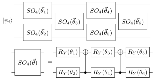
Figure 5: Ansatz quantum circuit for the VQE of the hydrogen molecule Parrish et al. (2019a). Each $\vec{\theta}$ has six parameters, and $R_{Y}(\theta)=e^{-i\frac{\theta}{2}Y}$. The total number of parameters is 36.

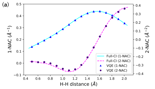
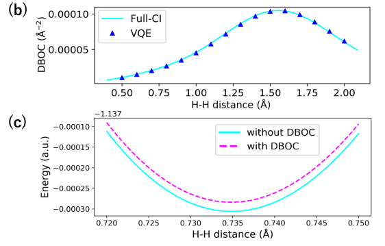
Figure 6: (a) Numerical results of calculating the 1-NAC $d_{02}$ and 2-NAC $D_{02}$ between $S_{0}$ state and $S_{2}$ state of the hydrogen molecule in bond lengths from $0.5\AA$ to $2.0\AA$ with the interval of $0.1\AA$. (b) Numerical results of calculating the DBOC of $S_{0}$ state of the hydrogen molecule from $0.5\AA$ to $2.0\AA$ with the interval of $0.1\AA$. (c) Numerical results of calculating potential energy curves by the VQE around the equilibrium distance of the hydrogen molecule without the DBOC (solid line) and with the DBOC (dashed line) from $0.7320\AA$ to $0.7350\AA$ with the interval of $0.0001\AA$. Including the DBOC shifts the equilibrium distance from $0.7349\AA$ to $0.7348\AA$. The NACs of “Full-CI” are obtained by numerical differentiation of the Full-CI results.

D.2 Berry’s phase of twisted 2-spin model

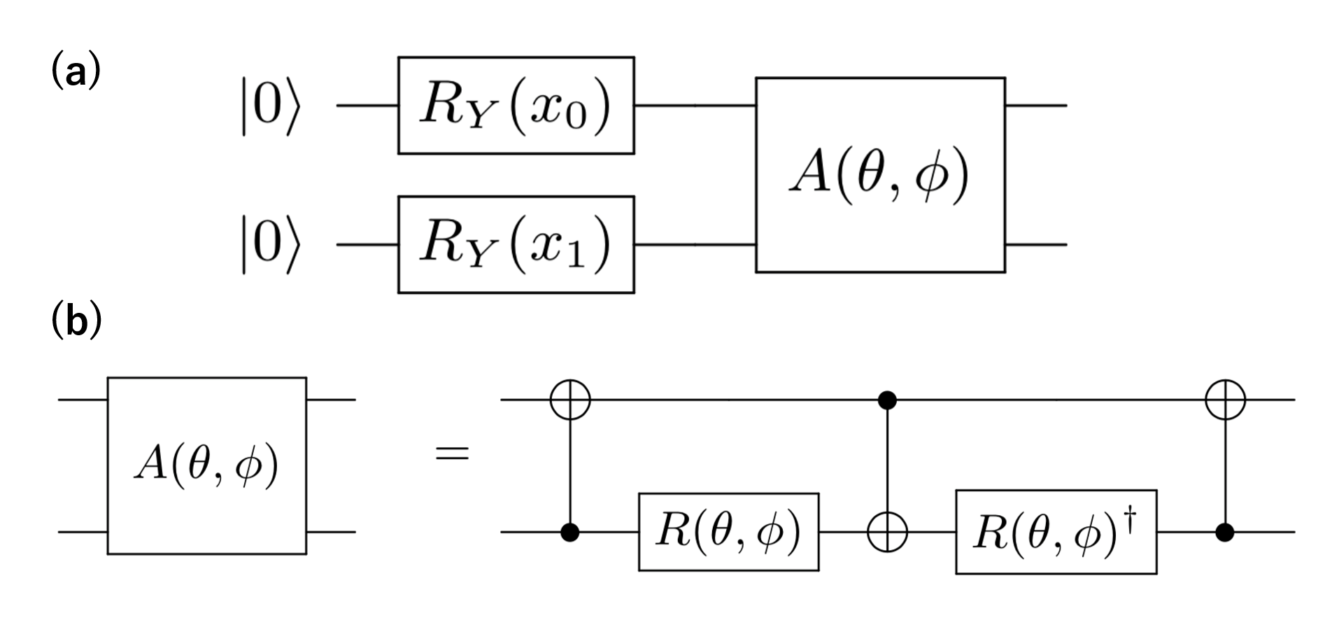
Figure 7: (a) Ansatz quantum circuit to find the ground state of Eq. (57). It contains four parameters $(x_{0},x_{1},\theta,\phi)$ to be optimized. (b) Definition of the particle-number-preserving gate $A(\theta,\phi)$ Gard et al. (2020). We define $R(\theta,\phi)$ as $R(\theta,\phi)=R_{Y}(\theta+\pi/2)R_{Z}(\phi+\pi)$, where $R_{Y}(\theta)=e^{i\theta Y/2}$ and $R_{Z}(\phi)=e^{i\phi Z/2}$.

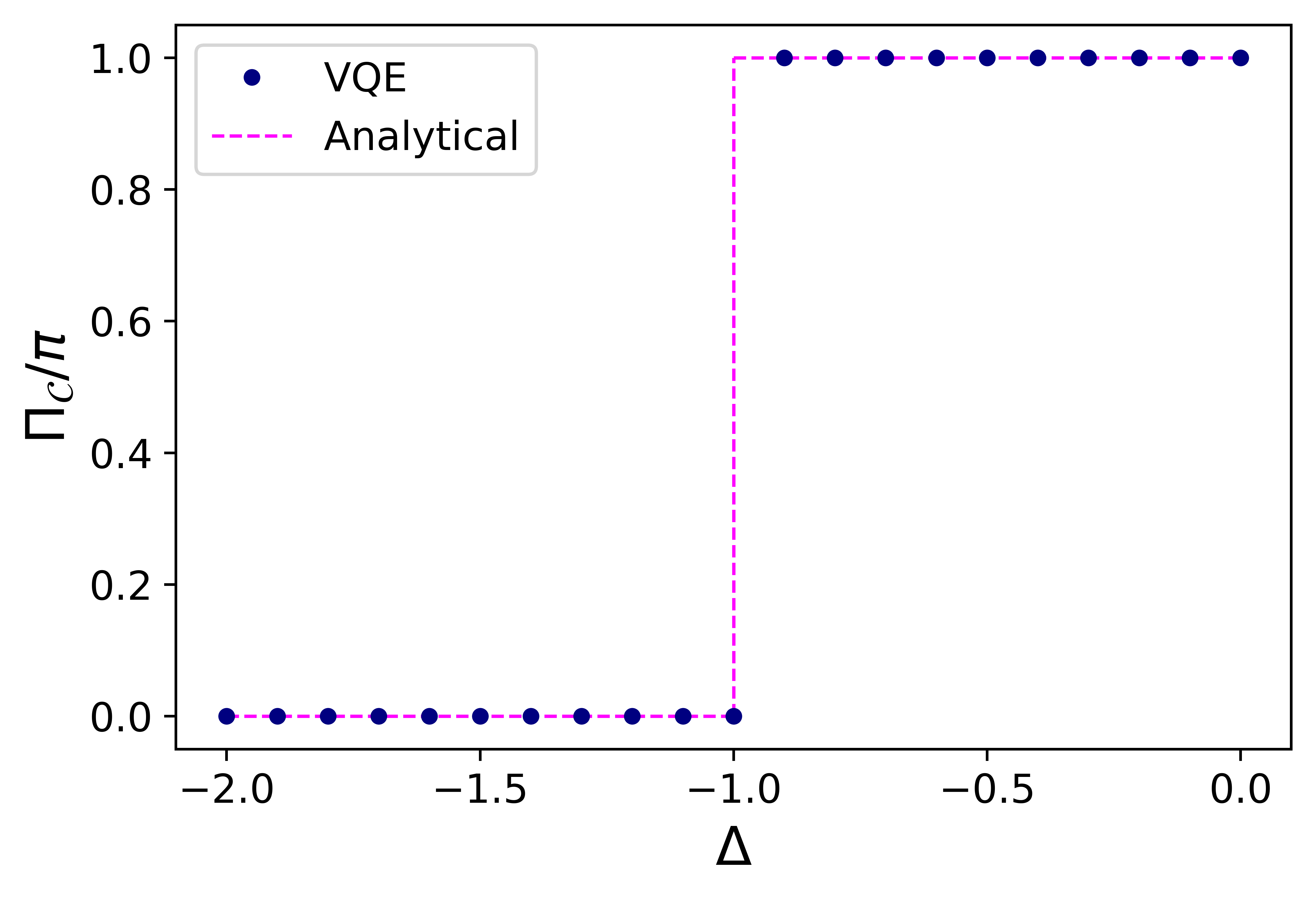
Figure 8: Numerical results of Berry’s phase $\Pi_{\mathcal{C}}$ of the model (57) based on Eq. (27) for the path $\rho=0\to 2\pi$ (dots). The analytical values of the model (57) (dashed line). We note that the numerical result when $\Delta=-1.0$ is unstable because of the degeneracy of the ground state.

To demonstrate our method for Berry’s phase, we use a two-site spin-1/2 model with a twist. The Hamiltonian is defined as

$$H_{\Delta}(\rho)=-\frac{1}{2}\left(e^{-i\rho}S_{0}^{+}S_{1}^{-}+e^{i\rho}S_{0}^{-}S_{1}^{+}\right)+\Delta S_{0}^{z}S_{1}^{z},$$ (57)

where $S_{i}^{\pm}=\frac{1}{2}(X_{i}\pm Y_{i})$, $S_{i}^{z}=\frac{1}{2}Z_{i}$, and $\rho$ is a twist angle. $\Delta$ is the parameter determines type and strength of the interaction between spins. The ground state for $-1<\Delta$ of this model is

$$\ket{\chi_{0}(\rho)}=\frac{1}{\sqrt{2}}\left(\ket{01}+e^{i\rho}\ket{10}\right),$$ (58)

while for $\Delta<-1$ it is degenerate as

$$\ket{\chi_{0}(\rho)}=\ket{00},\ket{11}.$$ (59)

Since $H(\rho=0)=H(\rho=2\pi)$, we can consider Berry’s phase $\Pi_{\mathcal{C}}$ associated to the closed path $\mathcal{C}$ from $\rho=0$ to $\rho=2\pi$. From the exact expression of the ground state above, the analytical values of $\Pi_{\mathcal{C}}$ can be calculate as $\Pi_{\mathcal{C}}=\pi$ for $-1<\Delta$ and $\Pi_{\mathcal{C}}=0$ for $\Delta<-1$. Berry’s phase $\Pi_{\mathcal{C}}$, in this case, is called the local $Z_{2}$ Berry’s phase and known to detect the topological nature of the ground state of quantum many-body systems Hatsugai (2006); Kariyado et al. (2018).

We perform the VQE for the model (57) with the ansatz depicted in Fig. 7. Again, the BFGS algorithm implemented in Scipy library Virtanen et al. (2020) is used and all quantum circuit simulations are run by Qulacs in the noiseless case. We discretize the path from $\rho=0$ as $\rho=2\pi$ into $100$ points uniformly and run the VQE at each point. The first term of Eq. (27) is calculated by the summation (30) and the phase difference $\arg(\braket{\varphi(\vec{\theta}^{*}_{\mathrm{s}})}{\varphi(\vec{\theta}^{*}_{\mathrm{t}})})$ in Eq. (27) is evaluated by the Hadamard test in Fig. 2. The result is shown in Fig. 8. The value of Berry’s phase $\Pi_{\mathcal{C}}$ exhibits the sharp transition reflecting the change of the ground state. These results illustrate the validity of our method to calculate Berry’s phase based on the VQE.

References

- Preskill (2018) John Preskill, “Quantum Computing in the NISQ era and beyond,” Quantum 2, 79 (2018).
- McArdle et al. (2020) Sam McArdle, Suguru Endo, Alán Aspuru-Guzik, Simon C. Benjamin, and Xiao Yuan, “Quantum computational chemistry,” Rev. Mod. Phys. 92, 015003 (2020).
- Cao et al. (2019) Yudong Cao, Jonathan Romero, Jonathan P. Olson, Matthias Degroote, Peter D. Johnson, Mária Kieferová, Ian D. Kivlichan, Tim Menke, Borja Peropadre, Nicolas P. D. Sawaya, Sukin Sim, Libor Veis, and Alán Aspuru-Guzik, “Quantum chemistry in the age of quantum computing,” Chemical Reviews 119, 10856–10915 (2019).
- Mitarai et al. (2018) K. Mitarai, M. Negoro, M. Kitagawa, and K. Fujii, “Quantum circuit learning,” Phys. Rev. A 98, 032309 (2018).
- Farhi and Neven (2018) Edward Farhi and Hartmut Neven, “Classification with quantum neural networks on near term processors,” arXiv:1802.06002 (2018).
- Havlíček et al. (2019) Vojtěch Havlíček, Antonio D. Córcoles, Kristan Temme, Aram W. Harrow, Abhinav Kandala, Jerry M. Chow, and Jay M. Gambetta, “Supervised learning with quantum-enhanced feature spaces,” Nature 567, 209–212 (2019).
- Kusumoto et al. (2021) Takeru Kusumoto, Kosuke Mitarai, Keisuke Fujii, Masahiro Kitagawa, and Makoto Negoro, “Experimental quantum kernel trick with nuclear spins in a solid,” npj Quantum Information 7, 94 (2021).
- Farhi et al. (2014) Edward Farhi, Jeffrey Goldstone, and Sam Gutmann, “A quantum approximate optimization algorithm,” arXiv preprint arXiv:1411.4028 (2014).
- Cong et al. (2019) Iris Cong, Soonwon Choi, and Mikhail D. Lukin, “Quantum convolutional neural networks,” Nature Physics 15, 1273–1278 (2019).
- Cerezo et al. (2020) M. Cerezo, Kunal Sharma, Andrew Arrasmith, and Patrick J. Coles, “Variational quantum state eigensolver,” (2020), arXiv:2004.01372 [quant-ph] .
- Romero et al. (2017) Jonathan Romero, Jonathan P Olson, and Alan Aspuru-Guzik, “Quantum autoencoders for efficient compression of quantum data,” Quantum Science and Technology 2, 045001 (2017).
- Sharma et al. (2020a) Kunal Sharma, Sumeet Khatri, M Cerezo, and Patrick J Coles, “Noise resilience of variational quantum compiling,” New Journal of Physics 22, 043006 (2020a).
- McClean et al. (2016) Jarrod R McClean, Jonathan Romero, Ryan Babbush, and Alán Aspuru-Guzik, “The theory of variational hybrid quantum-classical algorithms,” New Journal of Physics 18, 023023 (2016).
- Endo et al. (2020a) Suguru Endo, Zhenyu Cai, Simon C. Benjamin, and Xiao Yuan, “Hybrid quantum-classical algorithms and quantum error mitigation,” (2020a), arXiv:2011.01382 [quant-ph] .
- Peruzzo et al. (2014) Alberto Peruzzo, Jarrod McClean, Peter Shadbolt, Man-Hong Yung, Xiao-Qi Zhou, Peter J. Love, Alán Aspuru-Guzik, and Jeremy L. O’Brien, “A variational eigenvalue solver on a photonic quantum processor,” Nature Communications 5, 4213 (2014).
- O’Malley et al. (2016) P. J. J. O’Malley, R. Babbush, I. D. Kivlichan, J. Romero, J. R. McClean, R. Barends, J. Kelly, P. Roushan, A. Tranter, N. Ding, B. Campbell, Y. Chen, Z. Chen, B. Chiaro, A. Dunsworth, A. G. Fowler, E. Jeffrey, E. Lucero, A. Megrant, J. Y. Mutus, M. Neeley, C. Neill, C. Quintana, D. Sank, A. Vainsencher, J. Wenner, T. C. White, P. V. Coveney, P. J. Love, H. Neven, A. Aspuru-Guzik, and J. M. Martinis, “Scalable quantum simulation of molecular energies,” Phys. Rev. X 6, 031007 (2016).
- Kandala et al. (2017) Abhinav Kandala, Antonio Mezzacapo, Kristan Temme, Maika Takita, Markus Brink, Jerry M. Chow, and Jay M. Gambetta, “Hardware-efficient variational quantum eigensolver for small molecules and quantum magnets,” Nature 549, 242–246 (2017).
- Colless et al. (2018) J. I. Colless, V. V. Ramasesh, D. Dahlen, M. S. Blok, M. E. Kimchi-Schwartz, J. R. McClean, J. Carter, W. A. de Jong, and I. Siddiqi, “Computation of molecular spectra on a quantum processor with an error-resilient algorithm,” Phys. Rev. X 8, 011021 (2018).
- Hempel et al. (2018) Cornelius Hempel, Christine Maier, Jonathan Romero, Jarrod McClean, Thomas Monz, Heng Shen, Petar Jurcevic, Ben P. Lanyon, Peter Love, Ryan Babbush, Alán Aspuru-Guzik, Rainer Blatt, and Christian F. Roos, “Quantum chemistry calculations on a trapped-ion quantum simulator,” Phys. Rev. X 8, 031022 (2018).
- Kandala et al. (2019) Abhinav Kandala, Kristan Temme, Antonio D. Córcoles, Antonio Mezzacapo, Jerry M. Chow, and Jay M. Gambetta, “Error mitigation extends the computational reach of a noisy quantum processor,” Nature 567, 491–495 (2019).
- McClean et al. (2017) Jarrod R. McClean, Mollie E. Kimchi-Schwartz, Jonathan Carter, and Wibe A. de Jong, “Hybrid quantum-classical hierarchy for mitigation of decoherence and determination of excited states,” Phys. Rev. A 95, 042308 (2017).
- Nakanishi et al. (2019) Ken M. Nakanishi, Kosuke Mitarai, and Keisuke Fujii, “Subspace-search variational quantum eigensolver for excited states,” Phys. Rev. Research 1, 033062 (2019).
- Parrish et al. (2019a) Robert M. Parrish, Edward G. Hohenstein, Peter L. McMahon, and Todd J. Martínez, “Quantum computation of electronic transitions using a variational quantum eigensolver,” Phys. Rev. Lett. 122, 230401 (2019a).
- Jones et al. (2019) Tyson Jones, Suguru Endo, Sam McArdle, Xiao Yuan, and Simon C Benjamin, “Variational quantum algorithms for discovering hamiltonian spectra,” Phys. Rev. A 99, 062304 (2019).
- Higgott et al. (2019) Oscar Higgott, Daochen Wang, and Stephen Brierley, “Variational quantum computation of excited states,” Quantum 3, 156 (2019).
- Ollitrault et al. (2020) Pauline J. Ollitrault, Abhinav Kandala, Chun-Fu Chen, Panagiotis Kl. Barkoutsos, Antonio Mezzacapo, Marco Pistoia, Sarah Sheldon, Stefan Woerner, Jay M. Gambetta, and Ivano Tavernelli, “Quantum equation of motion for computing molecular excitation energies on a noisy quantum processor,” Phys. Rev. Research 2, 043140 (2020).
- Yoshioka et al. (2020) Nobuyuki Yoshioka, Yuya O. Nakagawa, Kosuke Mitarai, and Keisuke Fujii, “Variational quantum algorithm for nonequilibrium steady states,” Phys. Rev. Research 2, 043289 (2020).
- Liu et al. (2021) Huan-Yu Liu, Tai-Ping Sun, Yu-Chun Wu, and Guo-Ping Guo, “Variational quantum algorithms for steady states of open quantum systems,” (2021), arXiv:2001.02552 [quant-ph] .
- Mitarai et al. (2020) Kosuke Mitarai, Yuya O. Nakagawa, and Wataru Mizukami, “Theory of analytical energy derivatives for the variational quantum eigensolver,” Phys. Rev. Research 2, 013129 (2020).
- Parrish et al. (2019b) Robert M Parrish, Edward G Hohenstein, Peter L McMahon, and Todd J Martinez, “Hybrid quantum/classical derivative theory: Analytical gradients and excited-state dynamics for the multistate contracted variational quantum eigensolver,” arXiv:1906.08728 (2019b).
- O’Brien et al. (2019) Thomas E. O’Brien, Bruno Senjean, Ramiro Sagastizabal, Xavier Bonet-Monroig, Alicja Dutkiewicz, Francesco Buda, Leonardo DiCarlo, and Lucas Visscher, “Calculating energy derivatives for quantum chemistry on a quantum computer,” npj Quantum Information 5, 113 (2019), arXiv:1905.03742 [quant-ph] .
- Endo et al. (2020b) Suguru Endo, Iori Kurata, and Yuya O. Nakagawa, “Calculation of the green’s function on near-term quantum computers,” Phys. Rev. Research 2, 033281 (2020b).
- Lengsfield III and Yarkony (1992) Byron H. Lengsfield III and David R. Yarkony, “Nonadiabatic interactions between potential energy surfaces: Theory and applications,” in Advances in Chemical Physics (John Wiley & Sons, Ltd, 1992) Chap. 1, pp. 1–71.
- Yarkony (2012) David R. Yarkony, “Nonadiabatic quantum chemistry—past, present, and future,” Chemical Reviews 112, 481–498 (2012).
- Berry (1984) Michael Victor Berry, “Quantal phase factors accompanying adiabatic changes,” Proceedings of the Royal Society of London. A. Mathematical and Physical Sciences 392, 45–57 (1984).
- Xiao et al. (2010) Di Xiao, Ming-Che Chang, and Qian Niu, “Berry phase effects on electronic properties,” Rev. Mod. Phys. 82, 1959–2007 (2010).
- Cohen et al. (2019) Eliahu Cohen, Hugo Larocque, Frédéric Bouchard, Farshad Nejadsattari, Yuval Gefen, and Ebrahim Karimi, “Geometric phase from aharonov–bohm to pancharatnam–berry and beyond,” Nature Reviews Physics 1, 437–449 (2019).
- Tully (1990) John C. Tully, “Molecular dynamics with electronic transitions,” The Journal of Chemical Physics 93, 1061–1071 (1990).
- Tully (2012) John C. Tully, “Perspective: Nonadiabatic dynamics theory,” The Journal of Chemical Physics 137, 22A301 (2012).
- Tavernelli (2015) Ivano Tavernelli, “Nonadiabatic molecular dynamics simulations: Synergies between theory and experiments,” Accounts of Chemical Research 48, 792–800 (2015).
- Takatsuka et al. (2015) Kazuo Takatsuka, Takehiro Yonehara, Kota Hanasaki, and Yasuki Arasaki, Chemical Theory beyond the Born-Oppenheimer Paradigm (WORLD SCIENTIFIC, 2015).
- Nakahara (2003) Mikio Nakahara, Geometry, topology and physics (CRC Press, 2003).
- Born and Oppenheimer (1927) M. Born and R. Oppenheimer, “Zur quantentheorie der molekeln,” Annalen der Physik 389, 457–484 (1927).
- Asbóth et al. (2016) János K Asbóth, László Oroszlány, and András Pályi, A short course on topological insulators (Springer, 2016).
- Hatsugai (2006) Yasuhiro Hatsugai, “Quantized berry phases as a local order parameter of a quantum liquid,” Journal of the Physical Society of Japan 75, 123601 (2006).
- Kariyado et al. (2018) Toshikaze Kariyado, Takahiro Morimoto, and Yasuhiro Hatsugai, “ berry phases in symmetry protected topological phases,” Phys. Rev. Lett. 120, 247202 (2018).
- Araki et al. (2020) Hiromu Araki, Tomonari Mizoguchi, and Yasuhiro Hatsugai, “ berry phase for higher-order symmetry-protected topological phases,” Phys. Rev. Research 2, 012009 (2020).
- Cleve et al. (1998) R. Cleve, A. Ekert, C. Macchiavello, and M. Mosca, “Quantum algorithms revisited,” Proceedings of the Royal Society of London Series A 454, 339 (1998).
- Murta et al. (2020) Bruno Murta, G. Catarina, and J. Fernández-Rossier, “Berry phase estimation in gate-based adiabatic quantum simulation,” Phys. Rev. A 101, 020302 (2020).
- IBM (2020) “IBM Quantum Experience,” (2020), https://quantum-computing.ibm.com/ .
- Hellmann (1933) H. Hellmann, “Zur Rolle der kinetischen Elektronenenergie für die zwischenatomaren Kräfte,” Zeitschrift fur Physik 85, 180–190 (1933).
- Feynman (1939) R. P. Feynman, “Forces in molecules,” Phys. Rev. 56, 340–343 (1939).
- Ben-Nun et al. (2000) M. Ben-Nun, Jason Quenneville, and Todd J. Martínez, “Ab initio multiple spawning: Photochemistry from first principles quantum molecular dynamics,” The Journal of Physical Chemistry A 104, 5161–5175 (2000).
- Ben-Nun and Martínez (2002) Michal Ben-Nun and Todd. J. Martínez, “Ab initio quantum molecular dynamics,” in Advances in Chemical Physics (John Wiley & Sons, Ltd, 2002) pp. 439–512.
- Handy et al. (1986) Nicholas C. Handy, Yukio Yamaguchi, and Henry F. Schaefer, “The diagonal correction to the born–oppenheimer approximation: Its effect on the singlet–triplet splitting of ch2 and other molecular effects,” The Journal of Chemical Physics 84, 4481–4484 (1986).
- Valeev and Sherrill (2003) Edward F. Valeev and C. David Sherrill, “The diagonal born–oppenheimer correction beyond the hartree–fock approximation,” The Journal of Chemical Physics 118, 3921–3927 (2003).
- Ryabinkin et al. (2014) Ilya G. Ryabinkin, Loïc Joubert-Doriol, and Artur F. Izmaylov, “When do we need to account for the geometric phase in excited state dynamics?” The Journal of Chemical Physics 140, 214116 (2014).
- Gherib et al. (2016) Rami Gherib, Liyuan Ye, Ilya G. Ryabinkin, and Artur F. Izmaylov, “On the inclusion of the diagonal born-oppenheimer correction in surface hopping methods,” The Journal of Chemical Physics 144, 154103 (2016).
- Errea et al. (2004) L. F. Errea, L. Fernández, A. Macías, L. Méndez, I. Rabadán, and A. Riera, “Sign-consistent dynamical couplings between ab initio three-center wave functions,” The Journal of Chemical Physics 121, 1663–1669 (2004).
- Vibók et al. (2005) Ágnes Vibók, Gábor J Halász, Sándor Suhai, and Michael Baer, “Assigning signs to the electronic nonadiabatic coupling terms: The H2, O system as a case study,” The Journal of Chemical Physics 122, 134109 (2005).
- Miao et al. (2019) Gaohan Miao, Nicole Bellonzi, and Joseph Subotnik, “An extension of the fewest switches surface hopping algorithm to complex hamiltonians and photophysics in magnetic fields: Berry curvature and “magnetic” forces,” The Journal of Chemical Physics 150, 124101 (2019).
- Gard et al. (2020) Bryan T. Gard, Linghua Zhu, George S. Barron, Nicholas J. Mayhall, Sophia E. Economou, and Edwin Barnes, “Efficient symmetry-preserving state preparation circuits for the variational quantum eigensolver algorithm,” npj Quantum Information 6, 10 (2020).
- Lee et al. (2019) Joonho Lee, William J. Huggins, Martin Head-Gordon, and K. Birgitta Whaley, “Generalized unitary coupled cluster wave functions for quantum computation,” Journal of Chemical Theory and Computation 15, 311–324 (2019).
- Grimsley et al. (2019) Harper R. Grimsley, Sophia E. Economou, Edwin Barnes, and Nicholas J. Mayhall, “An adaptive variational algorithm for exact molecular simulations on a quantum computer,” Nature Communications 10, 3007 (2019).
- Tang et al. (2021) Ho Lun Tang, V. O. Shkolnikov, George S. Barron, Harper R. Grimsley, Nicholas J. Mayhall, Edwin Barnes, and Sophia E. Economou, “Qubit-ADAPT-VQE: An Adaptive Algorithm for Constructing Hardware-Efficient Ansätze on a Quantum Processor,” PRX Quantum 2, 020310 (2021).
- Matsuzawa and Kurashige (2020) Yuta Matsuzawa and Yuki Kurashige, “Jastrow-type decomposition in quantum chemistry for low-depth quantum circuits,” Journal of Chemical Theory and Computation 16, 944–952 (2020).
- Mitarai and Fujii (2019) Kosuke Mitarai and Keisuke Fujii, “Methodology for replacing indirect measurements with direct measurements,” Phys. Rev. Research 1, 013006 (2019).
- Note (1) The projective measurement of can be performed by applying a unitary gate which satisfies , executing the projective measurement of and finally applying after the projective measurement Mitarai and Fujii (2019). Such unitary can be constructed with depth, where is the number of qubits. First, we transform the non-identity part of into a product of gates by using gates and gates (note that ). Then CNOT gates are applied to make into by using the equality . Therefore, the depth of quantum gates needed is at most .
- Mukunda and Simon (1993) N. Mukunda and R. Simon, “Quantum kinematic approach to the geometric phase. i. general formalism,” Annals of Physics 228, 205–268 (1993).
- Note (2) Even if we choose the phase degree of freedom that depends on , the quantities that are evaluated on quantum devices to calculate Berry’s phase is the same. We consider the lift with , and the integrand of the first term can be written as . Integrating this term over gives additional terms with respect to the first term of Eq. (27\@@italiccorr), but, on the other hand, also gives rise to additional terms , which cancel each other out.
- Fukui et al. (2005) Takahiro Fukui, Yasuhiro Hatsugai, and Hiroshi Suzuki, “Chern numbers in discretized brillouin zone: Efficient method of computing (spin) hall conductances,” Journal of the Physical Society of Japan 74, 1674–1677 (2005).
- Virtanen et al. (2020) Pauli Virtanen, Ralf Gommers, Travis E. Oliphant, Matt Haberland, Tyler Reddy, David Cournapeau, Evgeni Burovski, Pearu Peterson, Warren Weckesser, Jonathan Bright, Stéfan J. van der Walt, Matthew Brett, Joshua Wilson, K. Jarrod Millman, Nikolay Mayorov, Andrew R. J. Nelson, Eric Jones, Robert Kern, Eric Larson, C. J. Carey, İlhan Polat, Yu Feng, Eric W. Moore, Jake VanderPlas, Denis Laxalde, Josef Perktold, Robert Cimrman, Ian Henriksen, E. A. Quintero, Charles R. Harris, Anne M. Archibald, Antônio H. Ribeiro, Fabian Pedregosa, Paul van Mulbregt, and SciPy 1. 0 Contributors, “SciPy 1.0: fundamental algorithms for scientific computing in Python,” Nature Methods 17, 261–272 (2020).
- Qis (2020) “Qiskit,” (2020), https://github.com/Qiskit .
- Werner and Meyer (1981) Hans Joachim Werner and Wilfried Meyer, “MCSCF study of the avoided curve crossing of the two lowest states of LiF,” The Journal of Chemical Physics 74, 5802–5807 (1981).
- Bauschlicher and Langhoff (1988) Charles W. Bauschlicher and Stephen R. Langhoff, “Full configuration-interaction study of the ionic-neutral curve crossing in LiF,” The Journal of Chemical Physics 89, 4246–4254 (1988).
- Bandrauk and Gauthier (1989) André D. Bandrauk and Jean Marc Gauthier, “Infrared multiphoton dissociation of LiF by a coupled equation method,” Journal of Physical Chemistry 93, 7552–7554 (1989).
- Bandrauk and Gauthier (1990) André D. Bandrauk and Jean-Marc Gauthier, “Above-threshold molecular photodissociation in ionic molecules: a numerical simulation,” J. Opt. Soc. Am. B 7, 1420–1427 (1990).
- Sun et al. (2017) Qiming Sun, Jun Yang, and Garnet Kin-Lic Chan, “A general second order complete active space self-consistent-field solver for large-scale systems,” Chemical Physics Letters 683, 291 – 299 (2017).
- Kuroiwa and Nakagawa (2021) Kohdai Kuroiwa and Yuya O. Nakagawa, “Penalty methods for a variational quantum eigensolver,” Phys. Rev. Research 3, 013197 (2021).
- Temme et al. (2017) Kristan Temme, Sergey Bravyi, and Jay M Gambetta, “Error mitigation for short-depth quantum circuits,” Physical review letters 119, 180509 (2017).
- Endo et al. (2018) Suguru Endo, Simon C Benjamin, and Ying Li, “Practical quantum error mitigation for near-future applications,” Physical Review X 8, 031027 (2018).
- Tully and Preston (1971) John C Tully and Richard K Preston, “Trajectory Surface Hopping Approach to Nonadiabatic Molecular Collisions: The Reaction of H+ with D2,” The Journal of Chemical Physics 55, 562–572 (1971).
- Mai et al. (2019) Sebastian Mai, Martin Richter, Moritz Heindl, Maximilian F. S. J. Menger, Andrew Atkins, Matthias Ruckenbauer, Felix Plasser, Lea Maria Ibele, Simon Kropf, Markus Oppel, Philipp Marquetand, and Leticia González, “Sharc2.1: Surface hopping including arbitrary couplings — program package for non-adiabatic dynamics,” sharc-md.org (2019).
- Richter et al. (2011) Martin Richter, Philipp Marquetand, Jesús González-Vázquez, Ignacio Sola, and Leticia González, “SHARC: ab initio molecular dynamics with surface hopping in the adiabatic representation including arbitrary couplings,” J. Chem. Theory Comput. 7, 1253–1258 (2011).
- Mai et al. (2018) Sebastian Mai, Philipp Marquetand, and Leticia González, “Nonadiabatic dynamics: The sharc approach,” WIREs Computational Molecular Science 8, e1370 (2018).
- Motta et al. (2018) Mario Motta, Erika Ye, Jarrod Mcclean, Zhendong Li, Austin Minnich, Ryan Babbush, and Garnet Chan, “Low rank representations for quantum simulation of electronic structure,” npj Quantum Information 7, 83 (2018).
- Huggins et al. (2021) William J. Huggins, Jarrod R. McClean, Nicholas C. Rubin, Zhang Jiang, Nathan Wiebe, K. Birgitta Whaley, and Ryan Babbush, “Efficient and noise resilient measurements for quantum chemistry on near-term quantum computers,” npj Quantum Information 7, 23 (2021).
- Baer (2006) Michael Baer, “Studies of molecular systems,” in Beyond Born–Oppenheimer: Electronic Nonadiabatic Coupling Terms and Conical Intersections (John Wiley & Sons, Ltd, 2006) Chap. 4, pp. 84–104.
- McClean et al. (2018) Jarrod R. McClean, Sergio Boixo, Vadim N. Smelyanskiy, Ryan Babbush, and Hartmut Neven, “Barren plateaus in quantum neural network training landscapes,” Nature Communications 9, 4812 (2018), arXiv:1803.11173 [quant-ph] .
- Cerezo et al. (2021) M. Cerezo, Akira Sone, Tyler Volkoff, Lukasz Cincio, and Patrick J. Coles, “Cost function dependent barren plateaus in shallow parametrized quantum circuits,” Nature Communications 12, 1791 (2021), arXiv:2001.00550 [quant-ph] .
- Cerezo and Coles (2021) M Cerezo and Patrick J Coles, “Higher order derivatives of quantum neural networks with barren plateaus,” Quantum Science and Technology 6, 035006 (2021).
- Uvarov and Biamonte (2021) A V Uvarov and J D Biamonte, “On barren plateaus and cost function locality in variational quantum algorithms,” Journal of Physics A: Mathematical and Theoretical 54, 245301 (2021).
- Sharma et al. (2020b) Kunal Sharma, M. Cerezo, Lukasz Cincio, and Patrick J. Coles, “Trainability of dissipative perceptron-based quantum neural networks,” (2020b), arXiv:2005.12458 [quant-ph] .
- Grant et al. (2019) Edward Grant, Leonard Wossnig, Mateusz Ostaszewski, and Marcello Benedetti, “An initialization strategy for addressing barren plateaus in parametrized quantum circuits,” Quantum 3, 214 (2019).
- Skolik et al. (2021) Andrea Skolik, Jarrod Mcclean, M. Mohseni, Patrick van der Smagt, and Martin Leib, “Layerwise learning for quantum neural networks,” Quantum Machine Intelligence 3, 5 (2021).
- Verdon et al. (2019) Guillaume Verdon, Michael Broughton, Jarrod R. McClean, Kevin J. Sung, Ryan Babbush, Zhang Jiang, Hartmut Neven, and Masoud Mohseni, “Learning to learn with quantum neural networks via classical neural networks,” (2019), arXiv:1907.05415 [quant-ph] .
- Anand et al. (2020) Abhinav Anand, Matthias Degroote, and Alán Aspuru-Guzik, “Natural evolutionary strategies for variational quantum computation,” (2020), arXiv:2012.00101 [quant-ph] .
- Pesah et al. (2020) Arthur Pesah, M. Cerezo, Samson Wang, Tyler Volkoff, Andrew T. Sornborger, and Patrick J. Coles, “Absence of barren plateaus in quantum convolutional neural networks,” (2020), arXiv:2011.02966 [quant-ph] .
- Bravyi and Kitaev (2002) Sergey B. Bravyi and Alexei Yu. Kitaev, “Fermionic quantum computation,” Annals of Physics 298, 210 – 226 (2002).
- Seeley et al. (2012) Jacob T. Seeley, Martin J. Richard, and Peter J. Love, “The bravyi-kitaev transformation for quantum computation of electronic structure,” The Journal of Chemical Physics 137, 224109 (2012), https://doi.org/10.1063/1.4768229 .
- Bravyi et al. (2017) Sergey Bravyi, Jay M Gambetta, Antonio Mezzacapo, and Kristan Temme, “Tapering off qubits to simulate fermionic hamiltonians,” arXiv:1701.08213 (2017).
- Sun et al. (2018) Qiming Sun, Timothy C. Berkelbach, Nick S. Blunt, George H. Booth, Sheng Guo, Zhendong Li, Junzi Liu, James D. McClain, Elvira R. Sayfutyarova, Sandeep Sharma, Sebastian Wouters, and Garnet Kin-Lic Chan, “Pyscf: the python-based simulations of chemistry framework,” WIREs Computational Molecular Science 8, e1340 (2018).
- McClean et al. (2020) Jarrod R McClean, Nicholas C Rubin, Kevin J Sung, Ian D Kivlichan, Xavier Bonet-Monroig, Yudong Cao, Chengyu Dai, E Schuyler Fried, Craig Gidney, Brendan Gimby, Pranav Gokhale, Thomas Häner, Tarini Hardikar, Vojtěch Havlíček, Oscar Higgott, Cupjin Huang, Josh Izaac, Zhang Jiang, Xinle Liu, Sam McArdle, Matthew Neeley, Thomas O’Brien, Bryan O’Gorman, Isil Ozfidan, Maxwell D Radin, Jhonathan Romero, Nicolas P D Sawaya, Bruno Senjean, Kanav Setia, Sukin Sim, Damian S Steiger, Mark Steudtner, Qiming Sun, Wei Sun, Daochen Wang, Fang Zhang, and Ryan Babbush, “OpenFermion: the electronic structure package for quantum computers,” Quantum Science and Technology 5, 034014 (2020).
- Hoeffding (1963) Wassily Hoeffding, “Probability inequalities for sums of bounded random variables,” Journal of the American Statistical Association 58, 13–30 (1963).
- Jordan and Wigner (1928) P. Jordan and E. Wigner, “Über das Paulische Äquivalenzverbot,” Zeitschrift fur Physik 47, 631–651 (1928).
- Suzuki et al. (2020) Yasunari Suzuki, Yoshiaki Kawase, Yuya Masumura, Yuria Hiraga, Masahiro Nakadai, Jiabao Chen, Ken M Nakanishi, Kosuke Mitarai, Ryosuke Imai, Shiro Tamiya, et al., “Qulacs: a fast and versatile quantum circuit simulator for research purpose,” arXiv preprint arXiv:2011.13524 (2020).