Remarks on ${\mathcal{H}}^{\infty}$ Controller Design for SISO Plants with Time Delays

Abstract

The skew Toeplitz approach is one of the well developed methods to design ${\mathcal{H}}^{\infty}$ controllers for infinite dimensional systems. In order to be able to use this method the plant needs to be factorized in some special manner. This paper investigates the largest class of SISO time delay systems for which the special factorizations required by the skew Toeplitz approach can be done. Reliable implementation of the optimal controller is also discussed. It is shown that the finite impulse response (FIR) block structure appears in these controllers not only for plants with I/O delays, but also for general time-delay plants.

1 Introduction

There are many well-developed techniques for finding ${\mathcal{H}}^{\infty}$ optimal and suboptimal controllers for systems with time delays. In particular, when the plant is a dead-time system: $e^{-hs}P_{0}(s)$ where $P_{0}$ is a rational SISO plant, the optimal ${\mathcal{H}}^{\infty}$ control problem is solved by Zhou and Khargonekar (1987), Foias et al. (1986), using operator theoretic methods; see also Smith (1989), Ozbay (1990) and their references. State-space solution to the same problem is given in Tadmor (1997), and Meinsma and Zwart (2000). Notably, Meinsma and Zwart (2000) used $J$-spectral factorization approach to solve the MIMO version of the problem. Moreover they showed the finite impulse response (FIR) structure appearing in the reliable implementation of the ${\mathcal{H}}^{\infty}$ controllers for dead-time systems. Meinsma and Mirkin (2005) extended this result to the multi-delay dead-time systems (input/output delay case).

A closed-form controller formula is obtained by Kashima and Yamamoto (2003) for the sensitivity minimization problem involving pseudorational plants. For more general infinite dimensional plants a solution is given by Foias et al. (1996). Their approach needs inner-outer factorization of the plant. Toker and Özbay (1995) simplified this method and brought into a compact form.

Kashima (2005) obtained an expression for the optimal ${\mathcal{H}}^{\infty}$ controller for the plants that can be expressed as a cascade connection of a finite-dimensional generalized plant and a scalar inner function. As it was done by Mirkin (2003), the solution is reduced to solving two algebraic Riccati equations and an additional one-block problem. Moreover, Kashima (2005) gave the inner-outer factorizations of stable pseudorational systems.

In our study, we determine the largest class of time-delay systems (TDS) for which the Skew-Toeplitz approach of Foias et al. (1996) is applicable. In order to use this method it is necessary to do inner-outer factorizations of the plant. An additional assumption is that the infinite dimensional plant has finitely many unstable zeros or poles. In this paper, we give necessary and sufficient conditions for TDS to have finitely many unstable zeros or poles. We classify the TDS and give conditions such that the desired factorization is possible. For admissible plants, the factorization is given and optimal ${\mathcal{H}}^{\infty}$ controller is obtained. The unstable pole-zero cancellation in the optimal controller expression of Toker and Özbay (1995) is eliminated. This way we establish the link between Toker and Özbay (1995) and Meinsma and Zwart (2000) by showing the FIR structure appearing in ${\mathcal{H}}^{\infty}$ controllers for not only dead-time plants, but also for more general TDS.

2 Preliminary Definitions and Results

In Foias et al. (1996); Toker and Özbay (1995), it is assumed that the plant is in the form

$$\hat{P}(s)=\frac{\hat{m}_{n}(s)\hat{N}_{o}(s)}{\hat{m}_{d}(s)}$$ (1)

where $\hat{m}_{n}(s)$ is inner, infinite dimensional and $\hat{m}_{d}(s)$ is inner, finite dimensional and $\hat{N}_{o}(s)$ is outer, possibly infinite dimensional. The optimal ${\mathcal{H}}^{\infty}$ controller, $\hat{C}_{opt}$, stabilizes the feedback system and achieves the minimum ${\mathcal{H}}^{\infty}$ cost, $\hat{\gamma}_{opt}$:

$$\hat{\gamma}_{opt}=\left\|\left[\begin{array}[]{c}\hat{W}_{1}(1+\hat{P}\hat{C}_{opt})^{-1}\\ \hat{W}_{2}\hat{P}\hat{C}_{opt}(1+\hat{P}\hat{C}_{opt})^{-1}\end{array}\right]\right\|_{\infty}$$ (2)

where $\hat{W}_{1}$ and $\hat{W}_{2}$ are finite dimensional weights of the mixed sensitivity minimization problem.

Recently, the optimal ${\mathcal{H}}^{\infty}$ control problem is solved by Gümüşsoy and Özbay (2004) for systems with infinitely many unstable poles and finitely many unstable zeros by using the duality with the problem (2). In this case, the plant has a factorization

$$\tilde{P}(s)=\frac{\tilde{m}_{d}(s)\tilde{N}_{o}(s)}{\tilde{m}_{n}(s)}$$ (3)

where $\tilde{m}_{n}$ is inner, infinite dimensional, $\tilde{m}_{d}(s)$ is finite dimensional, inner, and $\tilde{N}_{o}(s)$ is outer, possibly infinite dimensional. For this dual problem, the optimal controller, $\tilde{C}_{opt}$, and minimum ${\mathcal{H}}^{\infty}$ cost, $\tilde{\gamma}_{opt}$, are found for the mixed sensitivity minimization problem

$$\tilde{\gamma}_{opt}=\left\|\left[\begin{array}[]{c}\tilde{W}_{1}(1+\tilde{P}\tilde{C}_{opt})^{-1}\\ \tilde{W}_{2}\tilde{P}\tilde{C}_{opt}(1+\tilde{P}\tilde{C}_{opt})^{-1}\end{array}\right]\right\|_{\infty}.$$ (4)

In this paper we consider general delay systems:

$$P(s)=\frac{r_{p}(s)}{t_{p}(s)}=\frac{\sum_{i=1}^{n}r_{p,i}(s)e^{-h_{i}s}}{\sum_{j=1}^{m}t_{p,j}(s)e^{-\tau_{j}s}}$$ (5)

satisfying the assumptions

1. 1. $r_{p,i}(s)$ and $t_{p,j}(s)$ are polynomials with real coefficients;

   2. $h_{i}$, $\tau_{j}$ are rational numbers such that $0\leq h_{1}<h_{2}<\ldots<h_{n}$, and $0\leq\tau_{1}<\tau_{2}<\ldots<\tau_{m}$, with $h_{1}\geq\tau_{1}$;

   3. define the polynomials $r_{p,i_{max}}$ and $t_{p,j_{max}}$ with largest polynomial degree in $r_{p,i}$ and $t_{p,j}$ respectively (the smallest index if there is more than one), then, ${\textrm{deg}\{r_{p,i_{max}}(s)\}}\leq{\textrm{deg}\{t_{p,{j_{max}}}(s)\}}$ and $h_{i_{max}}\geq\tau_{j_{max}}$ where $\textrm{deg}\{.\}$ denotes the degree of the polynomial;

2. $P$ has no imaginary axis zeros or poles;

3. $P$ has finitely many unstable poles or zeros, or equivalently $r_{p}(s)$ or $t_{p}(s)$ has finitely many zeros in $\mathbb{C}_{+}$;

4. $P$ can be written in the form of (1) or (3).

Conditions stated in $A.1$ are not restrictive. In most cases $A.2$ can be removed if the weights are chosen in a special manner. The conditions $A.3-A.4$ come from the Skew-Toeplitz approach. It is not easy to check assumptions $A.3-A.4$, unless a quasi-polynomial root finding algorithm is used. We will give a necessary and sufficient condition to check the assumption $A.3$ in section 2.1 and give conditions to check the assumption $A.4$ in section 3.1.

By simple rearrangement, $P$ can be written as,

$$P(s)=\frac{R(s)}{T(s)}=\frac{\sum_{i=1}^{n}R_{i}(s)e^{-h_{i}s}}{\sum_{j=1}^{m}T_{j}(s)e^{-\tau_{j}s}}$$ (6)

where $R_{i}$ and $T_{j}$ are finite dimensional, stable, proper transfer functions. The assumptions $A.1-A.4$ and rearrangement of the plant are illustrated on the following example. Consider the system

$$\dot{x}_{1}(t) = -x_{1}(t-0.2)-x_{2}(t)+u(t)+2u(t-0.4),$$

$$\dot{x}_{2}(t) = 5x_{1}(t-0.5)-3u(t)+2u(t-0.4),$$

$$y(t) = x_{1}(t).$$ (7)

whose transfer function is in the form

$$P(s) = \frac{r_{p}(s)}{t_{p}(s)}=\frac{\sum_{i=1}^{2}r_{p,i}(s)e^{-h_{i}s}}{\sum_{i=1}^{3}t_{p,i}(s)e^{-\tau_{i}s}},$$ (8)

$$= \frac{(s+3)e^{-0s}+2(s-1)e^{-0.4s}}{s^{2}e^{-0s}+se^{-0.2s}+5e^{-0.5s}}.$$

Note that $r_{p,i}$ and $t_{p,j}$ are polynomials with real coefficients, delays are nonnegative with increasing order. By $i_{max}=1$ and $j_{max}=1$, $h_{1}=0\geq\tau_{1}=0$ and ${\textrm{deg}\{r_{p,1}(s)\}}=1\leq{\textrm{deg}\{t_{p,1}(s)\}}=2$. Therefore, assumption $A.1$ is satisfied. The plant, $P$ has no imaginary axis poles or zeros (assumption $A.2$). The denominator of the plant, $t_{p}(s)$ has finitely many unstable zeros at $0.4672\pm 1.8890j$, whereas $r_{p}(s)$ has infinitely many unstable zeros converging to $1.7329~{}-~{}(5k+2.5)\pi j$ as $k\rightarrow\infty$. Therefore, plant has finitely many unstable poles satisfying assumption $A.3$. One can show that the plant can be factorized as (1). In this example we have

$$P=\frac{R}{T}=\frac{\sum_{i=1}^{2}R_{i}(s)e^{-h_{i}s}}{\sum_{i=1}^{3}T_{j}(s)e^{-\tau_{i}s}}$$ (9)

where

$$R_{i}(s) = \frac{r_{p,i}(s)}{(s+1)^{2}},\quad\textrm{and}\quad T_{j}=\frac{t_{p,j}(s)}{(s+1)^{2}}$$

are stable proper finite dimensional transfer functions. Below we give conditions such that $A.3-A.4$ can be checked easily.

2.1 Time Delay Systems with Finitely Many Unstable Zeros or Poles

Definition 2.1

Consider $R(s)=\sum_{i=1}^{n}R_{i}(s)e^{-h_{i}s}$ where each $R_{i}$ is a rational, proper, stable transfer function with real coefficient, and $0\leq h_{1}<h_{2}<\ldots<h_{n}$. Let relative degree of $R_{i}(s)$ be $d_{i}$, then

• if $d_{1}<\max{\{d_{2},\ldots,d_{n}\}}$, then $R(s)$ is a retarded-type time-delay system (RTDS),

• if $d_{1}=\max{\{d_{2},\ldots,d_{n}\}}$, then $R(s)$ is a neutral-type time-delay system (NTDS),

• if $d_{1}>\max{\{d_{2},\ldots,d_{n}\}}$, then $R(s)$ is an advanced-type time-delay system (ATDS).

Note that if $R$ and $T$ are ATDS, plant has always infinitely many unstable zeros and poles which is not a valid plant for Skew-Toeplitz approach. It is well-known that RTDS has finitely unstable zeros on the right-half plane, Bellman and Cooke (1963). Therefore, we will give a necessary and sufficient condition to check whether a NTDS has finitely many or infinitely many unstable zeros with the following lemma:

Lemma 2.1

Assume that $R(s)$ is a NTDS with no imaginary axis zeros and poles, then the system, $R$, has finitely many unstable zeros if and only if all the roots of the polynomial, $\varphi(r)=1+\sum_{i=2}^{n}\xi_{i}r^{\tilde{h}_{i}-\tilde{h}_{1}}$ has magnitude greater than $1$ where

$$\xi_{i} = \lim_{\omega\rightarrow\infty}R_{i}(j\omega)R_{1}^{-1}(j\omega)\quad\forall\;i=2,\dots,n,$$

$$h_{i} = \frac{\tilde{h}_{i}}{N},\quad N,\tilde{h}_{i}\in\mathbb{Z}_{+},\;\forall\;i=1,\dots,n.$$

Proof. Since delays are rational numbers, there exist positive integers $N$ and $\tilde{h}_{i}$. If $R$ is a NTDS, there is no root with real part extending to infinity, i.e.,

$$\left|\frac{R(s)e^{h_{1}s}}{R_{1}(s)}\right|_{\sigma\rightarrow\infty}\geq 1-\lim_{\sigma\rightarrow\infty}\sum_{i=2}^{n}|\xi_{i}|e^{-(h_{i}-h_{1})\sigma}>0$$

where $s=\sigma+j\omega$. Therefore, NTDS may have infinitely many unstable zeros extending to infinity in imaginary part with bounded positive real part, see Bellman and Cooke (1963). $R$ has finitely many unstable zeros if and only if $R(\sigma+j\omega)$ has finitely many zeros as $\omega\rightarrow\infty$ and $0<\sigma<\sigma_{o}<\infty$. Equivalently, $R(\sigma+j\omega)$ has finitely many unstable zeros if and only if

$$\left.\lim_{\omega\rightarrow\infty}\frac{R(s)}{R_{1}(s)e^{-h_{1}s}}\right|_{s=\sigma_{o}+j\omega}=1+\sum_{i=2}^{n}\xi_{i}r^{\tilde{h}_{i}-\tilde{h}_{1}}$$ (10)

has finitely many unstable zeros where $r=e^{-\left(\frac{\sigma+j\omega}{N}\right)}$. Let $r_{0}$ is the root of (10). Then,

$$|r_{o}|=e^{-\sigma/N},\quad\sigma=-N\ln{|r_{o}|}.$$

Therefore, the system $R$ has finitely many unstable zeros if and only if all the roots of the polynomial (10) has magnitude greater than one. Note that if there exists a root $r_{o}$ of (10) with $|r_{o}|\leq 1$, then there are infinitely many unstable zeros of $R$ converging to $r_{o,k}=-\frac{\ln{|r_{o}|}}{N}-jN(\angle{r_{o}}+2\pi k)$ as $k\rightarrow\infty$ where $k\in\mathbb{Z}$ and $\angle{r_{o}}$ is the phase of the complex number $r_{o}$. $\Box$

Corollary 2.1

The time-delay system $R$ has finitely many unstable zeros if and only if $R$ is a RTDS or $R$ is a NTDS satisfying Lemma 2.1.

A time delay system with finitely many unstable zeros will be called an $F$-system. We define the conjugate of $R(s)=\sum_{i=1}^{n}R_{i}(s)e^{-h_{i}s}$ as $\bar{R}(s):=e^{-h_{n}s}R(-s)M_{C}(s)$ where $M_{C}$ is inner, finite dimensional whose poles are poles of $R$. For the above example, we have

$$R(s)=\frac{s+3+2(s-1)e^{-0.4s}}{(s+1)^{2}}$$

where $h_{1}=0$, $h_{2}=0.4$ and $M_{C}(s)=\left(\frac{s-1}{s+1}\right)^{2}$. So, the conjugate of $R(s)$ can be written as,

$$\bar{R}(s)=\frac{2(s+1)+(s-3)e^{-0.4s}}{(s+1)^{2}}.$$ (11)

Corollary 2.2

The time-delay system $\bar{R}$ has finitely many unstable zeros if and only if $R$ is a ATDS or $R$ is a NTDS with $\bar{R}$ satisfying Lemma 2.1.

The system $R$ whose conjugate $\bar{R}$ has finitely many unstable zeros is an $I$-system. Using Corollary 2.1, an equivalent condition for assumption $A.3$ is the following.

Corollary 2.3

Plant (6) has finitely many unstable zeros or poles if and only if $R$ or $T$ is an $F$-system.

Using Corollary 2.3, it is easy to check whether the plant has finitely many unstable or zeros. After putting the plant in the form (6), if $R$ or $T$ is RTDS, then assumption $A.3$ is satisfied; if $R$ or $T$ is NTDS and Lemma 2.1 is satisfied at least for one of them, then assumption $A.3$ holds.

It is well known that, since $R\in{\mathcal{H}}^{\infty}$, functions in the form $R$ admit inner outer factorizations

$$R=m_{n}N_{o}$$ (12)

where $m_{n}$ is inner and $N_{o}$ is outer. To illustrate this first assume that $R$ is an $F$-system. By Corollary 2.1, it has finitely many unstable zeros. Define an inner function $M_{R}$ whose zeros are unstable zeros of $R$. Note that $M_{R}$ is finite dimensional, rational function. Then, $R$ can be factorized as in (12) where $m_{n}=M_{R}$ and $N_{o}=\frac{R}{M_{R}}$. Note that unstable zeros of $R$ are cancelled by zeros of $M_{R}$, therefore $N_{o}$ is outer and $m_{n}$ is inner by construction of $M_{R}$. Similarly, if $R$ is an $I$-system, By Corollary 2.2, $\bar{R}$ has finitely many unstable zeros. Define an inner function $M_{\bar{R}}$ whose zeros are unstable zeros of $\bar{R}$. Using this result, $R$ can be factorized as in (12) where $m_{n}=\frac{R}{\bar{R}}M_{\bar{R}}$ and $N_{o}=\frac{\bar{R}}{M_{\bar{R}}}$.

Corollary 2.4

The plant $P=\frac{R}{T}$ satisfies $A.3-A.4$ if one of the following conditions are valid:

1. $R$ is $I$-system and $T$ is $F$-system (IF plant),

2. $R$ is $F$-system and $T$ is $I$-system (FI plant),

3. $R$ is $F$-system and $T$ is $F$-system (FF plant).

Proof. The TDS (6) should have finitely many unstable zeros or poles to apply Skew-Toeplitz approach. By Corollary 2.1, $R$ or $T$ should be a $F$-system which covers all the cases except $R$ and $T$ are $I$-systems. Recall that $P$ (6) can be factorized as

$$P=\frac{R}{T}=\frac{m_{n,R}N_{o,p}}{m_{n,T}N_{o,T}}=\frac{m_{n,R}}{m_{n,T}}N_{o}$$

where $N_{o}=\frac{N_{o,R}}{N_{o,T}}$ is outer function. Note that when $R$ is $F$ or $I$-system, $m_{n,R}$ is finite or infinite dimensional respectively. Similarly, when $T$ is $F$ or $I$-system, $m_{n,T}$ is finite or infinite dimensional respectively. Therefore, the plant (6) can be factorized as (1) or (3). $\Box$

Remarks:

1. By Corollary 2.4, it is easy to check whether assumptions $A.3-A.4$ are satisfied or not. For the plant (9) in the example, $T$ is a RTDS, by Corollary 2.1, $T$ is an $F$-system. $R$ is a NTDS and $\bar{R}$ satisfies Corollary 2.2, therefore, $R$ is a $I$-system, i.e., $\varphi(r)$ for $\bar{R}$ (11) is $1+\frac{1}{2}r$ and root of the polynomial has magnitude greater than $1$.

2. One can show that $R$ or $T$ has infinitely many imaginary-axis zeros if and only if corresponding $\varphi(r)$ has a root with magnitude $1$ in Lemma 2.1. Since by assumption $A.2$, $P$ has no imaginary axis poles or zeros, this possibility is eliminated. In fact, if plant $P$ does not have infinitely many imaginary-axis poles or zeros, the magnitude of roots of $\varphi(r)$ is never equal to $1$.

3. For a given system $R$, if magnitudes of all roots of $\varphi(r)$ in Lemma 2.1 are smaller than one, then $R$ is an $I$-system.

4. $R$ is an $F$-system $\Longleftrightarrow$ $\bar{R}$ is an $I$-system.

2.2 FIR Part of the Time Delay Systems

We now show a special structure of time delay systems. This key lemma is used in the next section.

Lemma 2.2

Let $R$ be as in Lemma 2.1 and $M_{R}$ be a finite dimensional system whose zeros are included in the zeros of $R$. Let $\mathcal{S}_{z}^{+}$ be the set of common $\mathbb{C}_{+}$ zeros of $R$ and $M_{R}$. Then $\frac{R}{M_{R}}$, can be decomposed as $\frac{R}{M_{R}}=H_{R}(s)+\mathcal{F}_{R}(s)$, where $H_{R}$ is a system whose poles are outside of $\mathcal{S}_{z}^{+}$ and the impulse response of $\mathcal{F}_{R}$ has finite support (by a slight abuse of notation we say $\mathcal{F}_{R}$ is an FIR filter).

Proof. For simplicity assume that $z_{1},z_{2},\dots,z_{n_{z}}\in\mathcal{S}_{z}^{+}$ are distinct. We can rewrite $\frac{R}{M_{R}}$ as $\frac{R}{M_{R}}=\sum_{i=1}^{n}\frac{R_{i}}{M_{R}}e^{-h_{i}s}$, and decompose each term by partial fraction, $\frac{R_{i}}{M_{R}}=H_{i}+F_{i}$ where the poles of $F_{i}$ are elements of $\mathcal{S}_{z}^{+}$ and define the terms $H_{R}$ and $\mathcal{F}_{R}$ as,

$$H_{R}(s)=\sum_{i=1}^{n}H_{i}(s)e^{-h_{i}s},\;\mathcal{F}_{R}(s)=\sum_{i=1}^{n}F_{i}(s)e^{-h_{i}s}.$$

where $F_{i}$ is strictly proper and $\mathcal{F}_{R}(z_{k})$ is finite $\forall\;i=1,\dots,n_{z}$. The lemma ends if we can show that $\mathcal{F}_{R}$ is FIR filter. Inverse Laplace transform of $\mathcal{F}_{R}$ can be written as,
$f_{R}(t)=\sum_{k=1}^{n_{z}}\left[\sum_{i=1}^{n}Res\{F_{i}(s)\}\Big{|}_{s=z_{k}}\;e^{z_{k}(t-h_{i})}u_{h_{i}}(t)\right]$ where $u_{h_{i}}(t)=u(t-h_{i})$, $u(t)$ and $Res(.)$ are unit step function and the residue of the function respectively. For $t>h_{n}$, we have
$f_{R}(t)=\sum_{k=1}^{n_{z}}e^{z_{k}t}\left[\sum_{i=1}^{n}Res\{F_{i}(s)\}\Big{|}_{s=z_{k}}\;e^{-h_{i}z_{k}}\right]$. Since, $Res\{F_{i}(s)\}\Big{|}_{s=z_{k}}=R_{i}(z_{k})Res\{M_{R}(s)\}\Big{|}_{s=z_{k}}$, $f_{R}(t)=\sum_{k=1}^{n_{z}}\left[e^{z_{k}t}Res\{M_{R}(s)\}\Big{|}_{s=z_{k}}R(z_{k})\right]\equiv 0$
for $t>h_{n}$ using the fact $\{z_{k}\}_{k=1}^{n_{z}}$ are the zeros of $R$. Therefore, we can conclude that $\mathcal{F}_{R}$ is a FIR filter with support $[0,h_{n}]$. Note that the above arguments are also valid for common zeros with multiplicities in $\mathcal{S}_{z}^{+}$. $\Box$

Note that this decomposition eliminates unstable pole-zero cancellation in $\frac{R}{M_{R}}$ and brings it into a form which is easy for numerical implementation. Lemma 2.2 explains the FIR part of the ${\mathcal{H}}^{\infty}$ controllers as shown below. Assume that $R$ is defined as in Definition 2.1 and $R_{0}$ is a bi-proper, finite dimensional system. By partial fraction, $\frac{R_{i}}{R_{0}}=R_{i,r}+R_{i,0}\quad\forall i=1,\dots,n$, where the $R_{i,0}$ is strictly proper transfer function whose poles are same as the zeros of $R_{0}$. Then, the decomposition operator, $\Phi$, is defined as,

$$\Phi(R,R_{0})=H_{R}+\mathcal{F}_{R}$$

where $H_{R}=\sum_{i=1}^{n}R_{i,r}e^{-h_{i}s}$ and $\mathcal{F}_{R}=\sum_{i=1}^{n}R_{i,0}e^{-h_{i}s}$ are infinite dimensional systems. Note that if the zeros of $R_{0}$ are also unstable zeros of $R$, then $\mathcal{F}_{R}$ is a FIR filter by Lemma 2.2.

3 Main Results

In this section, we construct the optimal ${\mathcal{H}}^{\infty}$ controller for the plant $P$, (6), satisfying assumptions $A.1-A.4$. By Corollary 2.4, the plant, $P=\frac{R}{T}$, is assumed to be either IF, FI or FF plant.

For each case, we will find optimal ${\mathcal{H}}^{\infty}$ controller and obtain a structure where there is no internal unstable pole-zero cancellation in the controller.

3.1 Factorization of the Plants

In order to apply the Skew- Toeplitz approach, we need to factorize the plant as in (1) or (3).

3.1.1 IF Plant Factorization

Assume that the plant in (6) satisfies $A.1-A.4$, and $R$ is $I$-system and $T$ is $F$-system. Then $P$ is in the form (1), where

$$\hat{m}_{n} = e^{-(h_{1}-\tau_{1})s}M_{\bar{R}}\frac{\{e^{h_{1}s}R\}}{\bar{R}},\quad\hat{m}_{d}=M_{T},$$

$$\hat{N}_{o} = \frac{\bar{R}}{M_{\bar{R}}}\frac{M_{T}}{\{e^{\tau_{1}s}T\}}.$$ (13)

where $M_{\bar{R}}$ is an inner function whose zeros are the unstable zeros of $\bar{R}(s)$. Since $R$ is $I$-system, conjugate of $R$ has finitely many unstable zeros, so $M_{\bar{R}}$ is well-defined. Similarly, zeros of $M_{T}$ are unstable zeros of $T$. Note that $\hat{m}_{n}$ and $\hat{m}_{d}$ are inner functions, infinite and finite dimensional respectively. $\hat{N}_{o}$ is an outer term.

3.1.2 FI Plant Factorization

Let the plant (6) satisfy $A.1-A.4$ (with $h_{1}=\tau_{1}=0$), and assume $R$ is $F$-system and $T$ is $I$-system. Then the plant $P$ can be factorized as in (3),

$$\tilde{m}_{n} = M_{\bar{T}}\frac{T}{\bar{T}},\quad\tilde{m}_{d}=M_{R}(s),\quad\tilde{N}_{o}=\frac{R}{M_{R}}\frac{M_{\bar{T}}}{\bar{T}}.$$

The zeros of $M_{R}$ are right half plane zeros of $R$. The unstable zeros of $\bar{T}(s)$ are the same as the zeros of $M_{\bar{T}}$. Similar to previous section, conjugate of $T$ has finitely many unstable zeros since $T$ is an $I$-system. The right half plane pole-zero cancellations in $\tilde{m}_{n}$ and $\tilde{N}_{o}$ will be eliminated in Section 3.2.2 by the method of Section 2.2.

3.1.3 FF Plant Factorization

Let $P=R/T$ satisfy $A.1-A.4$, with $R$ and $T$ being $F$-systems. In this case $P$ is in the from (1),

$$\hat{m}_{n} = e^{-(h_{1}-\tau_{1})s}M_{R},\quad\hat{m}_{d}=M_{T}(s),$$

$$\hat{N}_{o} = \frac{\{e^{h_{1}s}R\}}{M_{R}}\frac{M_{T}}{\{e^{\tau_{1}s}T\}}$$ (14)

where $M_{R}$ and $M_{T}$ are inner functions whose zeros are unstable zeros of $R$ and $T$ respectively. Note that when $h_{1}=\tau_{1}=0$, $\hat{m}_{n}$ is finite dimensional. Then, exact unstable pole-zero cancellations are possible in this case (except the ones in $\hat{N}_{o}$).

3.2 Optimal ${\mathcal{H}}^{\infty}$ Controller Design

Optimal ${\mathcal{H}}^{\infty}$ controllers for problems (2) and (4) are given in Toker and Özbay (1995) and Gümüşsoy and Özbay (2004) for the plants (1) and (3) respectively. Given the plant and the weighting functions, the optimal ${\mathcal{H}}^{\infty}$ cost, $\gamma_{opt}$ can be found as described in these papers. Then, one needs to compute transfer functions labeled as $E_{\gamma_{opt}}$, $F_{\gamma_{opt}}$ and $L$. Due to space limitations we skip this procedure, see Toker and Özbay (1995) and Gümüşsoy and Özbay (2004) for full details. Instead, we now simplify the structure of the controllers so that a reliable implementation is possible, i.e. there are no internal unstable pole-zero cancellations.

3.2.1 Controller Structure of IF Plants

By using the method in Toker and Özbay (1995); Foias et al. (1996), the optimal controller can be written as,

$$\hat{C}_{opt}=\frac{K_{\hat{\gamma}_{opt}}\left(\frac{e^{\tau_{1}s}T}{M_{T}}\right)}{\frac{\bar{R}}{M_{\bar{R}}}+e^{\tau_{1}s}RF_{\hat{\gamma}_{opt}}L}$$ (15)

where $K_{\hat{\gamma}_{opt}}=E_{\hat{\gamma}_{opt}}F_{\hat{\gamma}_{opt}}M_{T}L$. In order to obtain this structure of controller:

1. Do the necessary cancellations in $K_{\hat{\gamma}_{opt}}$,

2. Partition, $K_{\hat{\gamma}_{opt}}$ as, $K_{\hat{\gamma}_{opt}}=\theta_{\hat{\gamma}_{opt}}\theta_{T}$ where $\theta_{\hat{\gamma}_{opt}}$ is a bi-proper transfer function. The zeros of $\theta_{\hat{\gamma}_{opt}}$ are right half plane zeros of $E_{\hat{\gamma}_{opt}}M_{T}$,

3. By Lemma 2.2, obtain ($H_{T}$, $\mathcal{F}_{T}$), ($H_{R_{1}}$,$\mathcal{F}_{R_{1}}$) and ($H_{R_{2}}$, $\mathcal{F}_{R_{2}}$) using the partitioning operator,

   $$H_{T}+\mathcal{F}_{T} = \Phi(e^{\tau_{1}s}T\theta_{T},M_{T}),$$

   $$H_{R_{1}}+\mathcal{F}_{R_{1}} = \Phi(\bar{R},M_{\bar{R}}\theta_{\hat{\gamma}_{opt}}),$$

   $$H_{R_{2}}+\mathcal{F}_{R_{2}} = \Phi(e^{\tau_{1}s}RF_{\hat{\gamma}_{opt}}L,\theta_{\hat{\gamma}_{opt}}).$$

Then, the optimal controller has the form,

$$\hat{C}_{opt}=\frac{H_{T}+\mathcal{F}_{T}}{H_{\hat{\gamma}_{opt}}+\mathcal{F}_{\hat{\gamma}_{opt}}}$$ (16)

where $H_{T}$, $H_{\hat{\gamma}_{opt}}=H_{R_{1}}+H_{R_{2}}$ are TDS and $\mathcal{F}_{T}$, $\mathcal{F}_{\hat{\gamma}_{opt}}=\mathcal{F}_{R_{1}}+\mathcal{F}_{R_{2}}$ are FIR filters. The controller has no unstable pole-zero cancellations.

3.2.2 Controller Structure of FI Plants

After the data transformation is done shown as shown in Gümüşsoy and Özbay (2004) $\tilde{\gamma}_{opt}$, $E_{\tilde{\gamma}_{opt}}$, $F_{\tilde{\gamma}_{opt}}$ and $L$ can be found as in IF plant case. We can write the inverse of the optimal controller similar to (15):

$$\tilde{C}^{-1}_{opt}=\frac{K_{\tilde{\gamma}_{opt}}\left(\frac{R}{M_{R}}\right)}{\frac{\bar{T}}{M_{\bar{T}}}+TF_{\tilde{\gamma}_{opt}}L}$$ (17)

where $K_{\tilde{\gamma}_{opt}}=E_{\tilde{\gamma}_{opt}}F_{\tilde{\gamma}_{opt}}M_{R}L$. Similar to IF plant case, we can obtain a reliable controller structure:

1. Do the necessary cancellations in $K_{\tilde{\gamma}_{opt}}$,

2. Partition, $K_{\tilde{\gamma}_{opt}}$ as, $K_{\tilde{\gamma}_{opt}}=\theta_{\tilde{\gamma}_{opt}}\theta_{R}$ where $\theta_{\tilde{\gamma}_{opt}}$ is a bi-proper transfer function. The zeros of $\theta_{\tilde{\gamma}_{opt}}$ are unstable zeros of $E_{\tilde{\gamma}_{opt}}M_{R}$,

3. By Lemma 2.2, obtain ($H_{R}$, $\mathcal{F}_{R}$), ($H_{T,1}$,$\mathcal{F}_{T_{1}}$) and ($H_{T_{2}}$, $\mathcal{F}_{T_{2}}$) using the partitioning operator,

   $$H_{R}+\mathcal{F}_{R} = \Phi(R\theta_{R},M_{R}),$$

   $$H_{T_{1}}+\mathcal{F}_{T_{1}} = \Phi(\bar{T},M_{\bar{T}}\theta_{\tilde{\gamma}_{opt}}),$$

   $$H_{T_{2}}+\mathcal{F}_{T_{2}} = \Phi(TF_{\tilde{\gamma}_{opt}}L,\theta_{\tilde{\gamma}_{opt}}).$$

Then, the optimal controller has the form,

$$\tilde{C}_{opt}=\frac{H_{\tilde{\gamma}_{opt}}+\mathcal{F}_{\tilde{\gamma}_{opt}}}{H_{R}+\mathcal{F}_{R}}.$$ (18)

where $H_{R}$, $H_{\tilde{\gamma}_{opt}}=H_{T_{1}}+H_{T_{2}}$ are TDS and $\mathcal{F}_{R}$, $\mathcal{F}_{\tilde{\gamma}_{opt}}=\mathcal{F}_{T_{1}}+\mathcal{F}_{T_{2}}$ are FIR filters. The controller has no unstable pole-zero cancellations. Note that the optimal controller is dual case of IF plants, $R$ and $T$ are interchanged with $h_{1}=\tau_{1}=0$.

3.2.3 Controller Structure of FF Plants

Structure of FF plants is similar to that of IF plants. We can calculate $\hat{\gamma}_{opt}$, $E_{\hat{\gamma}_{opt}}$, $F_{\hat{\gamma}_{opt}}$, $L$ by the method in Toker and Özbay (1995); Foias et al. (1996) and write optimal controller as:

$$\hat{C}_{opt}=\frac{K_{\hat{\gamma}_{opt}}\frac{\{e^{\tau_{1}}T\}}{M_{T}(s)}}{\frac{\{e^{h_{1}s}R\}}{M_{R}}+e^{\tau_{1}s}RF_{\hat{\gamma}_{opt}}L}$$ (19)

where $K_{\hat{\gamma}_{opt}}=E_{\hat{\gamma}_{opt}}F_{\hat{\gamma}_{opt}}M_{T}L$. The optimal ${\mathcal{H}}^{\infty}$ controller structure can be found by following similar steps as in IF plants. The controller structure will be the same as in (16). Note that when $h_{1}=\tau_{1}=0$, since $\hat{m}_{n}$ in (3.1.3) is finite dimensional, it possible to cancel the zeros of $\theta_{\hat{\gamma}_{opt}}$ with denominator.

4 Example

We consider IF plant (2) and weights as $W_{1}(s)=\frac{2s+2}{10s+1}$ and $W_{2}(s)=0.2(s+1.1)$. After the plant is factorized as (3.1.1), the optimal ${\mathcal{H}}^{\infty}$ cost for two block problem (2) is $\hat{\gamma}_{opt}=0.7203$. The impulse responses of $\mathcal{F}_{T}$ and $\mathcal{F}_{\hat{\gamma}_{opt}}$, of the controller (16), are FIR as in Figures 1 and 2, respectively.

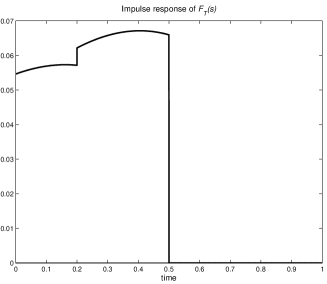
Figure 1: $f_{T}(t)$

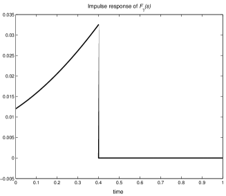
Figure 2: $f_{\hat{\gamma}_{opt}}(t)$

5 Concluding Remarks

In this paper we have discussed general time delay systems and defined FI, IF and FF types of plants. We showed how assumptions of the Skew Toeplitz theory can be checked, and illustrated numerically stable implementations of the optimal ${\mathcal{H}}^{\infty}$ controllers, avoiding internal pole-zero cancellations.

We should also mention that if the plant $P$ is written in terms of specific time delay factors, we may still design optimal ${\mathcal{H}}^{\infty}$ controllers even if $P$ is not in any of the types we have considered (i.e. IF, FI, and FF types). It is possible to design ${\mathcal{H}}^{\infty}$ controller for the following cases. Given the plant $P=\frac{R}{T}$, assume that $T$ is an $F$ system and $R$ is neither $F$ or $I$ system, but it can be factorized as $R=R_{F}R_{I}$ where $R_{F}$ is an $F$ system and $R_{I}$ is an $I$ system. Then, we can factorize the plant as (1),

$$\hat{m}_{n} = M_{R_{F}}M_{\bar{R}_{I}}\frac{R_{I}}{\bar{R}_{I}},\quad\hat{m}_{d}=M_{T},$$

$$\hat{N}_{o} = \left(\frac{R_{F}}{M_{R_{F}}}\right)\left(\frac{\bar{R}_{I}}{M_{\bar{R}_{I}}}\right)\left(\frac{M_{T}}{T}\right)$$

where $M_{R_{F}}$, $M_{\bar{R}_{I}}$ and $M_{T}$ are finite dimensional, inner functions whose zeros are unstable zeros of $R_{F}$, $\bar{R}_{I}$ and $T$ respectively. By this factorization, the optimal controller can be obtained as in (16). For the dual case, let $R$ be an $F$ system and $T=T_{F}T_{I}$ where $T_{F}$ is an $F$ system and $T_{I}$ is an $I$ system. Now the plant is in the form (3),

$$\tilde{m}_{n} = M_{R},\quad\tilde{m}_{d}=M_{T_{F}}M_{\bar{T}_{I}}\frac{T_{I}}{\bar{T}_{I}},$$

$$\tilde{N}_{o} = \left(\frac{R}{M_{R}}\right)\left(\frac{M_{T_{F}}}{T_{F}}\right)\left(\frac{M_{\bar{T}_{I}}}{\bar{T}_{I}}\right)$$

where $M_{R}$, $M_{\bar{T}_{I}}$ and $M_{T_{F}}$ are finite dimensional, inner functions whose zeros are unstable zeros of $R$, $\bar{T}_{I}$ and $T_{F}$ respectively. Now the optimal controller can be obtained as in (18).

Another interesting point to note is that the following plant is a special case of an FF system:

$$\dot{x}(t) = \sum_{i=1}^{n_{A}}A_{i}x(t-h_{A,i})+\sum_{j=1}^{n_{b}}b_{j}u(t-h_{b,j}),$$

$$y(t) = \sum_{k=1}^{n_{c}}c_{k}x(t-h_{c,k})+du(t-h_{d})$$ (20)

where $A_{i}\in{\mathbb{R}}^{n\times n}$, $b_{j}\in{\mathbb{R}}^{n\times 1}$, $c_{k}\in{\mathbb{R}}^{1\times n}$ and $d\in{\mathbb{R}}$. Define $x(t):=[x_{1}(t),\ldots,x_{n}(t)]^{T}$. The time-delays, $\{h_{A,i}\}_{i=1}^{n_{A}}$, $\{h_{b,i}\}_{i=1}^{n_{b}}$, $\{h_{c,i}\}_{i=1}^{n_{c}}$ are nonnegative rational numbers with ascending ordering respectively and $h_{d}\geq 0$. Therefore, we can design an optimal ${\mathcal{H}}^{\infty}$ controller for the plant (5) if there are no imaginary axis poles or zeros (or the weights are chosen in such a way that certain factorizations in Foias et al. (1996) can be done).

In general to see the plant type (IF, FI, FF), the transfer function should be obtained first, then using $R$ and $T$, one can decide the plant type by Corollary 2.1 and 2.2. The optimal ${\mathcal{H}}^{\infty}$ controller can be found by factorization of the plant and elimination of unstable pole-zero cancellations.

References

- Bellman and Cooke (1963) R. Bellman and K. L. Cooke, Differential-Difference Equations, 2.edn, pp. 342–348, New York: Academic Press.
- Foias et al. (1996) C. Foias, H. Özbay, A. Tannenbaum (1996). Robust Control of Infinite Dimensional Systems: Frequency Domain Methods, Lecture Notes in Control and Information Sciences, No. 209, Springer-Verlag, London.
- Foias et al. (1986) C. Foias, A. Tannenbaum and G. Zames (1986). “Weighted sensitivity minimization for delay systems,” IEEE Trans. Automatic Control, vol.31, pp.763–766.
- Gümüşsoy and Özbay (2004) S. Gümüşsoy and H. Özbay (2004). “On the Mixed Sensitivity Minimization for Systems with Infinitely Many Unstable Modes,” Syst. & Control Lett., vol. 53 no 3-4, pp. 211–216.
- Hirata et al. (2000) K. Hirata, Y. Yamamoto, and A. Tannenbaum (2000). “A Hamiltonian-based solution to the two-block problem for general plants in and rational weights,” Syst. & Control Lett., vol.40, pp. 83–96.
- Kashima (2005) K. Kashima, (2005). General solution to standard control problems for infinite-dimensional systems, Ph.D. Thesis, Kyoto University, Japan.
- Kashima and Yamamoto (2003) K. Kashima and Y. Yamamoto (2003). “Equivalent characterization of invariant subspaces of and applications to the optimal sensitivity problem,” Proc. of the IEEE Conf. on Decision and Control, vol.2, p.1824–1829.
- Meinsma and Mirkin (2005) G. Meinsma and L. Mirkin (2005). “ control of systems with multiple I/O delays via decomposition to adobe problems,” IEEE Trans. Automatic Control, vol.50, pp. 199–211.
- Meinsma and Zwart (2000) G. Meinsma and H. Zwart (2000). “On control for dead-time systems,” IEEE Trans. Automatic Control, vol.45, pp.272–285.
- Mirkin (2003) L. Mirkin (2003). “On the extraction of dead-time controllers and estimators from delay-free parameterizations,” IEEE Trans. Automatic Control, vol.48, pp.543–553.
- Ozbay (1990) H. Özbay (1990). “A simpler formula for the singular-values of a certain hankel operator,” Syst. & Control Lett., vol.15, pp.381–390.
- Ozbay et al. (1993) H. Özbay, M.C. Smith and A. Tannenbaum (1993). “Mixed-sensitivity optimization for a class of unstable infinite-dimensional systems,” Linear Algebra and its Applications, vol. 178, pp.43–83.
- Smith (1989) M.C. Smith (1989). “Singular-values and vectors of a class of hankel-operators,” Syst. & Control Lett., vol.12, pp.301–308.
- Tadmor (1997) G. Tadmor (1997). “Weighted sensitivity minimization in systems with a single input delay: A state space solution,” SIAM J. Control and Optimization, vol. 35, pp. 1445–1469.
- Toker and Özbay (1995) O. Toker and H. Özbay (1995). “ Optimal and suboptimal controllers for infinite dimensional SISO plants,” IEEE Trans. Automatic Control, vol.40, pp.751–755.
- Zhou and Khargonekar (1987) K. Zhou and P.P. Khargonekar (1987) “On the weighted sensitivity minimization problem for delay systems,” Syst. & Control Lett., vol.8, pp.307–312.