Divisors of Modular Parametrizations of Elliptic Curves

Abstract.

The modularity theorem implies that for every elliptic curve $E/\mathbb{Q}$ there exist rational maps from the modular curve $X_{0}(N)$ to $E$, where $N$ is the conductor of $E$. These maps may be expressed in terms of pairs of modular functions $X(z)$ and $Y(z)$ where $X(z)$ and $Y(z)$ satisfy the Weierstrass equation for $E$ as well as a certain differential equation. Using these two relations, a recursive algorithm can be used to calculate the $q$ - expansions of these parametrizations at any cusp. Using these functions, we determine the divisor of the parametrization and the preimage of rational points on $E$. We give a sufficient condition for when these preimages correspond to CM points on $X_{0}(N)$. We also examine a connection between the algebras generated by these functions for related elliptic curves, and describe sufficient conditions to determine congruences in the $q$-expansions of these objects.

1. Introduction and statement of results

The modularity theorem [12, 2] guarantees that for every elliptic curve $E$ of conductor $N$ there exists a weight $2$ newform $f_{E}$ of level $N$ with Fourier coefficients in $\mathbb{Z}$. The Eichler integral of $f_{E}$ (see (3)) and the Weierstrass $\wp$-function together give a rational map from the modular curve $X_{0}(N)$ to the coordinates of some model of $E.$ This parametrization has singularities wherever the value of the Eichler integral is in the period lattice. Kodgis [6] showed computationally that many of the zeros of the Eichler integral occur at CM points. Peluse [8] later proved several general cases confirming many of these conjectured zeros using the theory of Hecke operators and Atkin–Lehner involutions.

In [1], the authors use the modular parametrization of an elliptic curve to give a harmonic Maass form of weight $3/2$ whose Fourier coefficients encode the vanishing of central $L$-values and $L$-derivatives of quadratic twists of the curve. The Birch and Swinerton-Dyer conjecture asserts that the order of vanishing of the central $L$-value of an elliptic curve is the rank of the curve. Kolyvagin[7] confirmed this conjecture if the order of vanishing is less than $2$. Unfortunately, the result of [1] is only fully constructive if the modular parametrization is holomorphic on the upper half plane. Otherwise we must remove the singularities, a task which is difficult without knowledge of their locations.

For a modular function $F$ for some subgroup $\Gamma$ of $\operatorname{SL}_{2}(\mathbb{Z})$, we consider the modular polynomial of $F$

(1) $$\Phi_{F}(x):=\prod_{\gamma\in\Gamma\backslash SL_{2}(\mathbb{Z})}\Big{(}x-F(\gamma z)\Big{)}=\sum A_{i}(z)x^{i}.$$

One of our goals is to calculate the minimal divisor of $(\ref{ModPoly})$ for $F$ which are rational in terms of the coordinates functions $(X(z),Y(z))$ of a given modular parametrization of $E$, chosen so as to have poles at the divisor of the parametrization. We may calculate the divisor by calculating the divisor of the coefficient functions $A_{i}(z)$. In order to calculate the product in $(\ref{ModPoly})$ we need the expansion of $F$ at each of the cusps of $\Gamma$. Algorithms for calculating the coefficients of $X(z)$ and $Y(z)$ at the cusp infinity are described by Cremona [3], and we include a variation of that method that allows for the computation of coefficients at any cusp.

Example 1.1.

For the elliptic curve

(11a1) $$E:y^{2}+y=x^{3}-x^{2}-10x-20$$

one can calculate that $E$ has $(5,5)$ and $(5,-6)$ as points of order $5$. If we set $F(z)=\left(X(z)-5\right)^{-1}$, then $F(z)$ has zeros only when $z$ is an element of the complex lattice associated to $E$, and poles only when $z$ is mapped to one of these $5$-torsion points. Computing the divisor of $\Phi_{F}(X)$, we find that

$$X(z)=5\quad\implies\quad(j(z)+24729001)(j(z)+32768)=0.$$

If $z=\frac{1+\sqrt{-11}}{2}$, then $j(z)=-32768$. Since $j(z)$ is invariant under the action of $\operatorname{SL}_{2}(\mathbb{Z})$ while $F$ is only $\Gamma_{0}(11)$ invariant, we look at the $\Gamma_{0}(11)\backslash\operatorname{SL}_{2}(\mathbb{Z})$ orbit of $z$ to find

$$z_{0}=\frac{-11+\sqrt{-11}}{55}\quad\implies\quad\big{(}X(z_{0}),Y(z_{0})\big{)}=(5,5).$$

Thus the point $z_{0}$ is a preimage of the rational point $(5,5)$, and is a CM point on $X_{0}(11)$.

The points of $X_{0}(N)$ are in correspondence with pairs $(e,c)$ where $e$ is an elliptic curve and $c\subset e$ is a cyclic subgroup of order $N$ (See Appendix C.13 of [10]). Using this description, we give a sufficient condition for when a point $\mathcal{P}$ lying above a rational point $P$ on $E$ is a CM point. The proof is given in section $3$.

Theorem 1.2.

Fix an elliptic curve $E/\mathbb{Q}$ of conductor $N$ and $P$ a point on $E$. Let $\mathcal{P}$ a point on $X_{0}(N)$ that maps to $P$ under some modular parametrization, and which is in correspondence to the pair $(e,c)$ where $e$ is an elliptic curve over a number field $K$. For each $m\mid\mid N$, either $e$ admits an $m$-isogeny defined over $K$ or $e$ has CM by an order of discriminant $D$ where $0\leq-D\leq 4m$ and $D$ is a square $\pmod{4m}$.

In section $4$ we consider the question, given an elliptic curve $E$, when are the coefficients of these parametrizations contained in some prime ideal $\mathfrak{p}$ of a number ring $\mathcal{O}$? One sufficient condition we give is that the elliptic curves are isogenous, and have congruent coefficients mod $p$ for some prime $p$ lying below $\mathfrak{p}$. Another sufficient condition we provide is a bound similar to Sturm’s bound that implies that every coefficient of the parametrizations are in $\mathfrak{p}$ after a certain finite number of coefficients are.

2. Elliptic Curves

Given an elliptic curve $E$, we denote the periods of $E$ by $\omega_{1},\omega_{2}$, and the period lattice they generate by $\Lambda_{E}$. The Weierstrass $\wp$ function is defined in terms of $\Lambda_{E}$ and a complex variable $z$ as follows:

$$\wp(z,\Lambda_{E}):=\frac{1}{z^{2}}+\sum_{\begin{subarray}{c}\lambda\in\Lambda_{E}\\ \lambda\neq 0\end{subarray}}\frac{1}{(z+\lambda)^{2}}-\frac{1}{\lambda^{2}}.$$

The $\wp$-function $\wp(z,\Lambda_{E})$ is even as a function of $z$, and its defining series is absolutely convergent and doubly periodic with periods $\omega_{1},\omega_{2}$. The functions $\wp(z,\Lambda_{E})$ and $\wp^{\prime}(z,\Lambda_{E})$ satisfy the relation

(2) $$\wp^{\prime}(z,\Lambda_{E})^{2}=4\wp(z,\Lambda_{E})^{3}-g_{2}\wp(z,\Lambda_{E})-g_{3},$$

where

$$g_{2}=g_{2}(\Lambda_{E})=60\sum_{\begin{subarray}{c}\lambda\in\Lambda_{E}\\ \lambda\neq 0\end{subarray}}(\lambda)^{-4}$$

and

$$g_{3}=g_{3}(\Lambda_{3})=140\sum_{\begin{subarray}{c}\lambda\in\Lambda_{E}\\ \lambda\neq 0\end{subarray}}(\lambda)^{-6}.$$

Also associated $E$ is the canonical differential

$$\omega=mf_{E}(z)dz,$$

where $m$ is the Manin constant and $f_{E}$ is the weight two cusp form associated to $E$. The Eichler integral is then defined as

(3) $$\varepsilon(z)=\int_{z}^{i\infty}\omega=\int_{z}^{i\infty}mf_{E}(\tau)d\tau.$$

The function $\varepsilon(z)$ is not modular, but if $\gamma=\left(\begin{smallmatrix}a&b\\ c&d\end{smallmatrix}\right)\in\Gamma_{0}(N)$ acts as usual on the upper-half plane, then

$$\frac{d}{dz}\big{(}\varepsilon(\gamma z)-\varepsilon(z)\big{)} =\frac{d}{dz}2\pi i\int_{\gamma z}^{z}mf_{E}(\tau)d\tau$$

$$=2\pi im\big{(}f_{E}(z)-(cz+d)^{2}f_{E}(z)(cz+d)^{-2}\big{)}=0$$

where the second to last equality follows from the fundamental theorem of calculus and the modularity of $f_{E}$. So $\varepsilon(z)$ is almost modular, in that the difference $\varepsilon(\gamma z)-\varepsilon(z)$ depends only on $\gamma$, and not on $z$. Denote this difference by

$$C(\gamma):=\varepsilon(\gamma z)-\varepsilon(z).$$

One readily verifies that $C:\Gamma_{0}(N)\rightarrow m\Lambda_{E}$ is a group homomorphism. Eichler and Shimura [4, 9] showed that when the Manin constant is $1$, that $C$ is actually an isomorphism.

For any $\lambda\in\mathbb{C}$ such that $\lambda\in\textnormal{End}(E)$, we have that $\lambda\Lambda_{E}\subseteq\Lambda_{E}$. So it is possible to define

$$\wp_{\lambda}(z,\Lambda_{E}):=\lambda^{2}\wp(\lambda z,\Lambda_{E})=\wp(z,\frac{1}{\lambda}\Lambda_{E}),$$

where the extra factor $\lambda^{2}$ normalizes $\wp_{\lambda}$ to have a leading coefficient of $q^{-2}$ in its Fourier expansion. Similarly,

$$\wp_{\lambda}^{\prime}(z,\Lambda_{E}):=\lambda^{3}\wp^{\prime}(\lambda z,\Lambda_{E})=\wp^{\prime}(z,\frac{1}{\lambda}\Lambda_{E}).$$

With this notation we define

$$X_{\lambda}(z)=m^{2}\wp_{\lambda}(\varepsilon(z),\Lambda_{E})-\frac{a_{1}^{2}+4a_{2}}{12},$$

$$Y_{\lambda}(z)=\frac{m^{3}}{2}\wp_{\lambda}^{\prime}(\varepsilon(z),\Lambda_{E})-\frac{a_{1}m^{2}}{2}\wp_{\lambda}(\varepsilon(z),\Lambda_{E})+\frac{a_{1}^{3}+4a_{1}a_{2}-12a_{3}}{24}$$

for $E$ given in general Weierstrass form with the convention that if the subscript $\lambda$ is omitted we take $\lambda=1$. Note that if $E$ is given in Wierstrass short form then

$$X_{\lambda}(z):=m^{2}\wp_{\lambda}(\varepsilon(z),\Lambda_{E})\quad Y_{\lambda}(z):=\frac{m^{3}}{2}\wp_{\lambda}^{\prime}(\varepsilon(z),\Lambda_{E}).$$

By construction $X_{\lambda}(z),Y_{\lambda}(z)$ satisfy the Wierstrass equation for the elliptic curve. Importantly, $X_{\lambda}(z)$ and $Y_{\lambda}(z)$ are modular over $\Gamma_{0}(N)$ since

$$\wp_{\lambda}(\varepsilon(\gamma z),\Lambda_{E})=\wp_{\lambda}(\varepsilon(z)+C(\gamma),\Lambda_{E})=\wp_{\lambda}(\varepsilon(z),\Lambda_{E})$$

where the final equality holds because $\lambda C(\gamma)\in\Lambda_{E}$. A similar calculation holds for $Y_{\lambda}(z)$ as well as the parametrizations for the general form.

3. Expansions at Other Cusps

The first step in computing the coefficient functions $A_{i}$ in $(\ref{ModPoly})$ is to compute the $q$-expansions of each of the factors $(x-F(\gamma z))$ for $x$ a formal variable and $\gamma\in\operatorname{SL}_{2}(\mathbb{Z})$. Since we are interested specifically in $F$ that are rational functions of $X_{\lambda}(z)$ and $Y_{\lambda}(z)$ it suffices to calculate the $q$-expansions for $X(\gamma z)$ and $Y(\gamma z)$. These coefficients are determined by two relations,

(4) $$qX^{\prime}=(2Y+a_{1}X+a_{3})f_{E}$$

known as the invarient differential of $E$(see section III of [10]), and the elliptic curve relation

(5) $$Y^{2}+a_{1}XY+a_{3}Y=X^{3}+a_{2}X^{2}+a_{4}X+a_{6}.$$

A recursive algorithm was given by Cremona [3] using these two relations to calculate the expansions of $X(z)$ and $Y(z)$. Acting on $(\ref{defEichler})$ and $(\ref{DifRel})$ by a matrix $\gamma\in\operatorname{SL}_{2}(\mathbb{Z})$ gives relations that allow us to recursively calculate the coefficients of modular parametrizations around cusps other than infinity. There are, however, a few complications we examine below.

If we let $q_{N}(z)=e^{\frac{2\pi i}{N}z}$, we can write the expansions of the modular parametrizations at a cusp $\rho$ with width $w$ as $X_{\lambda}(\gamma z)=\sum_{n=-2}^{\infty}b_{n}q_{w}^{n}$ and $Y_{\lambda}(\gamma z)=\sum_{n=-3}^{\infty}d_{n}q_{w}^{n}$. Note that $b_{i},d_{i}$ might be zero for $i=-3,-2,-1$ if neither $X$ nor $Y$ have poles at $\rho$. By examining the first few terms if the Laurent series of $\wp_{\lambda}$ and $\wp_{\lambda}^{\prime}$ and evaluating them at $\varepsilon(\gamma z)$ we can calculate $b_{-2}$ and $d_{-3}$. So our inductive set up will be to assume that we know the $b_{i}$ coefficients for $-2\leq i\leq n-1$ and the $d_{j}$ coefficients for $-3\leq j\leq n-2$ and use this information to calculate $b_{n}$ and $d_{n-1}$. Letting $c_{n}$ denote the coefficient of $q_{w}^{n}$ of $f_{E}(\gamma z)$, relation $(\ref{defEichler})$ gives us that

$$\frac{1}{w}\sum_{n=-2}^{\infty}nb_{n}q_{w}^{n}=\Big{(}2\sum_{n=-3}^{\infty}d_{n}q_{w}^{n}+a_{1}\sum_{n=-2}^{\infty}b_{n}q_{w}^{n}+a_{3}\Big{)}\sum_{n=1}^{\infty}c_{n}q_{w}^{n}.$$

Comparing the coefficients of $q_{w}^{n}$ gives us one linear relation between $b_{n}$ and $d_{n-1}$

$$nb_{n}=2w\sum_{k=-3}^{n-1}c_{n-k}d_{k}+a_{1}w\sum_{k=-2}^{n-1}c_{n-k}b_{k}+a_{3}wc_{n}.$$

Comparing the $q_{w}^{n-4}$ term in $(\ref{DifRel})$ gives us

$$\sum_{k=-3}^{n-1}d_{n-4-k}d_{k}+a_{1}\sum_{k=-3}^{n-4}b_{n-4-k}d_{k}+a_{3}d_{n-4}=\\ \sum_{k=-2}^{n}\sum_{j=-2}^{n-2-k}b_{n-4-k-j}b_{j}b_{k}+a_{2}\sum_{k=-2}^{n-2}b_{n-4-j}b_{j}+a_{4}b_{n-4}+a_{6}^{*}$$

where $a_{6}^{*}$ indicates that this term is present only if $n-4=0$. This gives a second linear relation between $d_{n-1}$ and $b_{n}$, which allows us to solve for $d_{n-1}$ and $b_{n}$ uniquely whenever the determinant of the system is not $0$, i.e. when $-2nd_{-3}^{2}+6wc_{1}b_{-2}^{2}\not=0$. Supposing that $X_{\lambda}(z)$ has a pole at $\rho$, (so that neither $d_{-3}$ nor $b_{-2}$ are $0$), then

$$-2n(d_{-3})^{2}+6wc_{1}(b_{-2})^{2}=0\quad\implies n=\frac{3wc_{1}(b_{-2})^{2}}{(d_{-3})^{2}}.$$

So this recursive process will not fail if we can find the first $\frac{3wc_{1}(b_{-2})^{2}}{(d_{-3}^{2})}$ nontrivial terms of $X(z)$ and $Y(z)$ via the Laurent series expansions of $\wp_{\lambda}$ and $\wp_{\lambda}^{\prime}$. Note that when $\rho=\infty$, we have that $w=c_{1}=b_{-2}=d_{-3}=1$ so that Cremona’s algorithm doesn’t fail with simply $3$ known terms of the Laurent expansion of $\wp_{\lambda}(\varepsilon(z))$.

However, if there are no poles at $\rho$, then $d_{-3}=b_{-2}=0$, and the determinant will be $0$ for all $n$. So when calculating the $q_{w}$-expansions around cusps without poles, we need to compare other powers of $q_{w}$ to get information about such systems. Fortunately, we can simply compare powers of $q_{w}^{n}$ in $(\ref{defEichler})$ and $(\ref{DifRel})$ to get that a system with determinant $n(2d_{0}+a_{1}b_{0}+a_{3})$.

Interestingly, this determinant is zero when $2d_{0}+a_{1}b_{0}+a_{3}=0$, i.e when the constant terms of the expansions give a point of order $2$ on $E$. This is seen most easily by looking at $(\ref{defEichler})$, and observing that $2d_{0}+a_{1}b_{0}+a_{3}=0$ corresponds to a vertical tangent line on $E$. However, this is easily rectified. We first take $2d_{0}+a_{1}b_{0}+a_{3}=0$ as a hypothesis and compare powers of $q_{w}^{n}$ in $(\ref{defEichler})$ and powers of $q_{w}^{n}$ in $(\ref{DifRel})$ exactly like the previous case. The main difference is that since $2d_{0}+a_{1}b_{0}+a_{3}=0$, this gives us a system in the unknowns $b_{n}$ and $d_{n-1}$ instead of in terms of $b_{n}$ and $d_{n}$. So by examining $3$ cases we can effectively calculate the $q_{w}$-expansions of the modular parametrizations $X(z)$ and $Y(z)$ around any cusp.

Now that we can efficiently calculate these $q$-expansions for $X(\gamma z),Y(\gamma z)$ it is possible to construct

$$\Phi_{F}(x):=\prod_{\gamma\in\Gamma_{0}(N)\backslash SL_{2}(\mathbb{Z})}\Big{(}x-F(\gamma z)\Big{)}=\sum A_{i}(z)x^{i}$$

where $x$ is a formal variable and $F$ is any rational function in $X_{\lambda}(z)$ and $Y_{\lambda}(z)$. Note that by construction, the coefficients of $\Phi_{F}(x)$ are modular functions which are invariant under the action of $\operatorname{SL}_{2}(\mathbb{Z})$, and so are rational functions in Klein’s $j$-function.

In practice, in order to compute the minimal divisor of $\Phi_{F}(x)$ it is computationally advantageous to compute each of the functions $F(\gamma z)$ and then use symmetric polynomials to calculate the necessary coefficient functions until we locate all the poles of $F$.

Example 3.1.

Consider the elliptic curve

(26b1) $$E:y^{2}+xy+y=x^{3}-x^{2}-3x+3.$$

The point $(1,0)$ lies on $E$ and has $(1,-2)$ as its inverse. Then looking at the function $F(z)=\frac{Y(z)+2}{X(z)-1}$, we see that $F$ has a simple pole at the values $z\in\mathcal{H}$ that map $(X(z),Y(z))$ to $(1,0)$. Note that the conductor of $E$ is $26$, and $[\operatorname{SL}_{2}(\mathbb{Z}):\Gamma_{0}(26)]=42$. Calculating the trace of $\Phi_{F}$ (or the coefficient $A_{41}(z)$) we get

$$\sum_{\gamma\in\Gamma_{0}(26)\backslash\operatorname{SL}_{2}(\mathbb{Z})}F(\gamma z)=\frac{-j(z)^{2}+54688j(z)-37627200}{j(z)-54000}.$$

Testing the $42$ cosets of $\Gamma_{0}(26)$ in $\operatorname{SL}_{2}(\mathbb{Z})$ gives us that for $z_{0}=\frac{-7+\sqrt{-3}}{52}$, $\left(X(z_{0}),Y(z_{0})\right)=(1,0)$. Thus the preimage of the rational point $(1,0)$ is a CM point on $X_{0}(26)$.

Using this theory we are able to give a condition for when a point $P$ on an elliptic curve $E$ is the image of a CM point $\mathcal{P}$ on the modular curve and prove Theorem $1.2$.

Proof.

Suppose that $m$ exactly divides $N$ and let $\mathcal{P}_{2}=(e_{2},c_{2})$ be the image of $\mathcal{P}_{1}=(e_{1},c_{1})$ under the Atkin-Lehner involution $W_{m}=\left(\begin{smallmatrix}am&b\\ cN&dm\end{smallmatrix}\right)$ for integers $a,b,c,d$. The matrix $W_{m}$ imposes a rational map from $X_{0}(N)$ to itself, so if $e_{1}$ is not isomorphic to $e_{2}$, then $W_{m}$ is a rational isogeny of the curves $e_{1}$ and $e_{2}$. If $e_{1}$ is isomorphic to $e_{2}$ and we write the periods for $e_{1}$, $e_{2}$ as $\omega_{11},\omega_{12}$ and $\omega_{21},\omega_{22}$ respectively, then $W_{m}$ takes $\tau_{1}=\frac{\omega_{12}}{\omega_{11}}$ to $\tau_{2}=\frac{\omega_{22}}{\omega_{21}}$. However, since $e_{1}\cong e_{2}$, there must be a matrix $A=\left(\begin{smallmatrix}\alpha&\beta\\ \gamma&\delta\end{smallmatrix}\right)$ in $\operatorname{SL}_{2}(\mathbb{Z})$ such that $W_{m}\tau_{1}=\tau_{2}=A\tau_{1}$. This gives a quadratic relation that $\tau_{1}$ satisfies, namely

$$(am\tau_{1}+b)(\gamma\tau_{1}+\delta)=(\alpha\tau_{1}+\beta)(cN\tau_{1}+dm).$$

Expanding and collecting like terms gives

$$(am\gamma-c\alpha N)\tau_{1}^{2}+(b\gamma+am\delta-cN\beta-dm\alpha)\tau_{1}+b\delta-dm\beta=0.$$

The discriminant of this quadratic is

$$D =(b\gamma+am\delta-cN\beta-dm\alpha)^{2}-4(am\gamma-c\alpha N)(b\delta-dm\beta)$$

$$=b^{2}\gamma^{2}+a^{2}m^{2}\delta^{2}+c^{2}N^{2}\beta^{2}+d^{2}m^{2}\alpha^{2}$$

$$+2b\gamma am\delta-2b\gamma cN\beta-2b\gamma dm\alpha-2am\delta cN\beta-2adm^{2}\alpha\delta+2cN\beta dm\alpha$$

$$-4(am\gamma b\delta-am^{2}d\beta\gamma-cNb\alpha\delta+c\alpha Ndm\beta).$$

We collect like terms and use the fact that $\det(W_{m})=adm^{2}-cNb=m$ to get

$$D =b^{2}\gamma^{2}+a^{2}m^{2}\delta^{2}+c^{2}N^{2}\beta^{2}+d^{2}m^{2}\alpha^{2}$$

$$-2b\gamma am\delta+2b\gamma cN\beta-2b\gamma dm\alpha-2am\delta cN\beta+2adm^{2}\alpha\delta-2cN\beta dm\alpha$$

$$-4(m\alpha\delta-m\beta\gamma).$$

Factoring and using that $\det(A)=\alpha\delta-\beta\gamma=1$ gives that

$$D =(b\gamma-am\delta+cN\beta-dm\alpha)^{2}-4m.$$

Thus $D$ is a square mod $4m$. Since $\tau_{1}$ is in the upper half plane, we must have that $D<0$. However, since $(b\gamma-am\delta+cN\beta-dm\alpha)^{2}$ is non-negative, it follows that $-4m\leq D<0$. ∎

Example 3.2.

We return to the curve

(26b1) $$E:y^{2}+xy+y=x^{3}-x^{2}-3x+3$$

of conductor $26$ and index $42$. Consider the points $(1,-2)$ and $(3,2)$ with inverses $(1,0)$ and $(3,-6)$ on $E$. Then the functions $F$ and $G$ given by

$$F(z)=\frac{Y(z)-0}{X(z)-1},\quad G(z)=\frac{Y(z)+6}{X(z)-3}$$

have simple poles for $z$ such that $(X(z),Y(z))=(1,-2)$ or $(3,2)$ respectively. We calculate specific coefficient functions of $\Phi_{F}=\sum A_{i}(z)x^{i}$ and $\Phi_{G}=B_{i}(z)x^{i}$ to determine the location of these poles in the upper half plane:

$$A_{41}(z) =\frac{-j(z)^{2}+288156\cdot j(z)-199626768}{j(z)-287496},$$

$$B_{40}(z) =\frac{j(z)^{3}-3214\cdot j(z)^{2}+2726620\cdot j-274323456}{j(z)-1728}.$$

Thus $\Phi_{F}(z)$ has poles only when $j(z)=287496$, i.e when $z$ is in the $\operatorname{SL}_{2}(\mathbb{Z})$ orbit of $\sqrt{-4}$, and $G(z)$ has poles only when $j(z)=1728$ i.e when $z$ is in the $\operatorname{SL}_{2}(\mathbb{Z})$ orbit of $\sqrt{-1}$. Comparing the actions of the coset representatives of $\Gamma_{0}(26)$, we find that $z_{0}:=\frac{-5+\sqrt{-1}}{52}$ satisfies $(X(z),Y(z))=(1,-2)$, and $z_{1}=\frac{5+\sqrt{-1}}{13}$ satisfies $(X(z),Y(z))=(3,2)$.

Examining the action of the Atkin-Lehner involutions $W_{2}$ and $W_{13}$, we find that $F_{2}=F(W_{2}z)$ , and $G_{2}=G(W_{2}z)$ have coefficient functions

$$A_{40}(z)=\frac{-j(z)^{2}+3235\cdot j(z)-2655936}{j(z)-1728},\quad\quad B_{41}(z)=\frac{-42\cdot j(z)+21954240}{j(z)-287496},$$

while $F_{13}:=F(W_{13}z)$ and $G_{13}:=G(W_{13}z)$ have coefficient functions

$$A_{41}(z) =\frac{-j(z)^{2}+288156\cdot j(z)-199626768}{j(z)-287496},$$

$$B_{40}(z) =\frac{j(z)^{3}-3214\cdot j(z)^{2}+2726620\cdot j-274323456}{j(z)-1728}.$$

Thus since $W_{2}$ exchanges the poles of $F$ and $G$, Theorem $1.2$ gives that the points $z_{0}$, $z_{1}$ correspond to isogenous elliptic curves on $X_{0}(26)$. Additionally, since $W_{13}$ fixes $z_{0}$ and $z_{1}$, Theorem $1.2$ also tells us they are both CM points on $X_{0}(26)$ whose orders have discriminants that must be squares mod $52$. In fact, the minimal polynomial of $z_{0}$ is $104z^{2}-20z+1$ which has discriminant $-16\equiv 6^{2}\mod 52$, and the minimal polynomial for $z_{1}$ is $13z^{2}-10z+2$ which has discriminant $-4\equiv 10^{2}\mod 52$.

Example 3.3.

Theorem $1.2$ can also be visualized in the following way. Consider again the elliptic curve $E:y^{2}+y=x^{3}-x^{2}-10x-20$ of conductor $11$, and the fundamental domain $F_{11}$ in figure $1$ for the congruence subgroup $\Gamma_{0}(11)$.

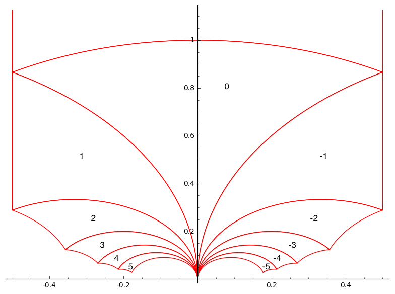
Figure 1. fundamental domain $F_{11}$ for $\Gamma_{0}(11)$

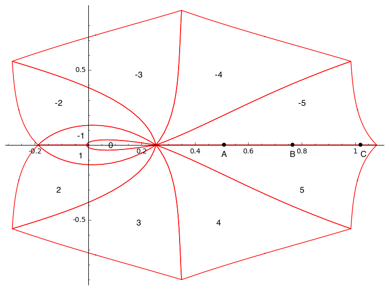
Figure 2. Eichler integral over the boundary of $F_{11}$

This fundamental domain has been constructed by taking $\operatorname{SL}_{2}(\mathbb{Z})$ coset representatives of the form $\left(\begin{smallmatrix}0&-1\\ 1&j\end{smallmatrix}\right)$ for $-5\leq j\leq 5$, with each $j$ labeled in the corresponding hypertriangle. The associated newform of $E$ is $f_{E}=q-2q^{2}-q^{3}+2q^{4}\dots$. Taking complex values $z$ on the boundary of $F_{11}$ and calculating $\varepsilon(z)=\int_{z}^{i\infty}mf_{E}(\tau)d\tau$ gives the image in Figure $2$. The resulting image tiles the plane in a parallelogram-type pattern, with the same periods as $E$. The points $A,B$ and $C$ have been labeled at $2/5$, $3/5$ and $4/5$ times the real period of $E$ respectively. They correspond to the points $(5,-6),(5,5)$ and $(16,60)$ on $E$ respectively. The action of $W_{11}$ interchanges the two cusps in Figure $2$ ($\infty$ located at the origin, and $0$ located at the value $.2538\dots$ on the real line which is $1/5$ the real period of $E$). Up to translation by the real period, we see that $W_{11}$ interchanges the points $A$ and $C$ but fixes point $B$. By Theorem $1.2$ we conclude that the preimages of the points $(5,-6)$ and $(16,60)$ on $X_{0}(11)$ give isogenous elliptic curves, while the preimage of $(5,5)$ on $X_{0}(11)$ must be a CM point as we saw in Example $1.1$.

4. Congruences Between Generated Algebras

Consider the elliptic curves $E_{1}$, $E_{2}$ given by

(14a1) $$E_{1}:y^{2}+xy+y =x^{3}+4x-6,$$

(14a2) $$E_{2}:y^{2}+xy+y =x^{3}-36x-70.$$

These curves have coefficients that are congruent mod $8$ and interestingly, if we look at the $q$-expansions of the row reduced basis elements of $\mathbb{Q}[X(z),Y(z)]$, we notice a similar phenomenon.

Basis over $E_{1},$ $X=X_{E_{1}}(z)$, $Y=Y_{E_{1}}(z)$	$q$-expansion
$1$				$1$
$X(z)-2$	$q^{-2}$	$+q^{-1}$	$+2q$	$+2q^{2}$	$+3q^{3}$	$+\cdots$
$-Y(z)-2X(z)-2$	$q^{-3}$	$+2q^{-1}$	$+5q$	$+4q^{2}$	$+2q^{3}$	$+\cdots$
$X(z)^{2}+2Y(z)-X(z)+2$	$q^{-4}$	$-q^{-1}$	$-2q$	$+8q^{2}$	$+5q^{3}$	$+\cdots$
$-Y(z)X(z)-3X(z)^{2}+2Y(z)+3X(z)-2$	$q^{-5}$		$-2q$	$-4q^{2}$	$+18q^{3}$	$+\cdots$
$X(z)^{3}+3X(z)Y(z)-5Y(z)+2X(z)-6$	$q^{-6}$	$-2q^{-1}$	$+4q$	$-7q^{2}$	$-6q^{3}$	$+\cdots$
Basis over $E_{2},$ $X=X_{E_{2}}(z)$, $Y=Y_{E_{2}}(z)$	$q$-expansion
$1$				$1$
$X(z)-2$	$q^{-2}$	$+q^{-1}$	$+2q$	$10q^{2}$	$-5q^{3}$	$+\cdots$
$-Y(z)-2X(z)-2$	$q^{-3}$	$+2q^{-1}$	$-3q$	$-4q^{2}$	$+2q^{3}$	$+\cdots$
$X(z)^{2}+2Y(z)-X(z)-14$	$q^{-4}$	$-q^{-1}$	$+14q$		$+29q^{3}$	$+\cdots$
$-Y(z)X(z)-3X(z)^{2}+2Y(z)+3X(z)+38$	$q^{-5}$		$+6q$	$-28q^{2}$	$-14q^{3}$	$+\cdots$
$X(z)^{3}+3X(z)Y(z)-5Y(z)-22X(z)-6$	$q^{-6}$	$-2q^{-1}$	$-12q$	$+25q^{2}$	$+138q^{3}$	$+\cdots$

The coefficients of the $q$-expansions are also congruent mod $8$. This is not simply a consequence of the congruence of the equations of $E_{1}$ and $E_{2}$. For example, the curves

(15a3) $$E_{3}:y^{2}+xy+y =x^{3}+x^{2}-5x+2,$$

(15a4) $$E_{4}:y^{2}+xy+y =x^{3}+x^{2}+35x-28.$$

are congruent mod $10$, but the $q$ expansions of the $X$ term of their optimal modular parametrizations are

$$X_{E_{3}}(z) =q^{-2}+q^{-1}+1+2q+3q^{2}+\hskip 6.02249ptq^{3}+\cdots-6q^{11}+\cdots,$$

$$X_{E_{4}}(z) =q^{-2}+q^{-1}+1+2q-5q^{2}+9q^{3}+\cdots+7q^{11}+\cdots.$$

Comparing the $q^{2}$ terms shows that any congruence between these two parametrizations must divide $8$, and comparing the $q^{11}$ terms shows that any such congruence must divide $13$. Thus we conclude that there are no nontrivial congruences between the parametrizations. So when do congruences in the elliptic curve equation give rise to congruences in the generated algebras?

If we assume that the two elliptic curves $E_{1}$ and $E_{2}$ given by

$$E_{1}:y^{2}+a_{1}xy+a_{3}y =x^{3}+a_{2}x^{2}+a_{4}x+a_{6},$$

$$E_{2}:y^{2}+\alpha_{1}xy+\alpha_{3}y =x^{3}+\alpha_{2}x^{2}+\alpha_{4}x+\alpha_{6},$$

are isogenous, then their period lattices will intersect nontrivially in a lattice $\Lambda_{3}$, corresponding to an elliptic curve $E_{3}$ with integral model

$$y^{2}+\beta_{1}xy+\beta_{3}y=x^{3}+\beta_{2}x^{2}+\beta_{4}x+\beta_{6}.$$

Thus the difference

$$g(z):=\wp(z,\Lambda_{1})-\wp(z,\Lambda_{2})$$

is an even, elliptic function with period lattice $\Lambda_{3}$. If we let $\{r_{i}\}$ represent the complex numbers such that $\wp(r_{i},\Lambda_{3})$ is a zero of $g(z)$ in a fundamental parallelogram of $\Lambda_{3}$ and let $\{t_{j}\}$ be the values in $\Lambda_{3}$ such that $\wp(t_{j},\Lambda_{3})$ is a pole of $g(z)$ (repeated according to multiplicities) except possibly at the origin (even if the origin is a zero or pole of $g$), then the function

$$\frac{\prod_{i}\left(\wp(z,\Lambda_{3})-\wp(r_{i},\Lambda_{3})\right)}{\prod_{j}(\wp(z,\Lambda_{3})-\wp(t_{j},\Lambda_{3}))}$$

is monic, and has the same zeros and poles as $g(z)$ except possibly at $0$. However, a classical arguement shows that the product must have the same zero or pole as $g(z)$ at $0$ as well (see [5] for example). Thus

(6) $$g(z)=\wp(z,\Lambda_{1})-\wp(z,\Lambda_{2})=C\frac{\prod_{i}(\wp(z,\Lambda_{3})-\wp(r_{i},\Lambda_{3}))}{\prod_{j}(\wp(z,\Lambda_{3})-\wp(t_{j},\Lambda_{3}))}$$

for some constant $C$. Since

$$\wp(z,\Lambda_{1})-\wp(z,\Lambda_{2})=\frac{g_{2}(\Lambda_{1})-g_{2}(\Lambda_{2})}{20}z^{2}+\frac{g_{3}(\Lambda_{1})-g_{3}(\Lambda_{2})}{28}z^{4}+\cdots$$

we see that

$$C=C(\Lambda_{1},\Lambda_{2})=\begin{cases}\frac{g_{2}(\Lambda_{1})-g_{2}(\Lambda_{2})}{20}&\text{ if }g_{2}(\Lambda_{1})\neq g_{2}(\Lambda_{2})\\ \frac{g_{3}(\Lambda_{1})-g_{3}(\Lambda_{2})}{28}&\text{ if }g_{2}(\Lambda_{1})=g_{2}(\Lambda_{2}).\end{cases}$$

With this notation we have the following.

Theorem 4.1.

Suppose that $E_{1},E_{2}$ are two isogenous elliptic curves over $\mathbb{Q}$. Also assume that the coordinates of the torsion points of order dividing $N$ in $\overline{\mathbb{Q}}$ are algebraic integers. Then there is an explicit natural number $D(\Lambda_{1},\Lambda_{2})$ so that the $q$-expansion of $X_{E_{1}}-X_{E_{2}}$ is congruent to a constant mod $C(\Lambda_{1},\Lambda_{2})/D(\Lambda_{1},\Lambda_{2})$.

Proof.

Evaluating equation (6) at $\varepsilon(z)$, and adding the appropriate constant to both sides of the equality gives

$$X_{E_{1}}(z)-X_{E_{2}}(z) =\wp(\varepsilon(z),\Lambda_{1})+\frac{a_{1}^{2}-4a_{2}}{12}-\wp(\varepsilon(z),\Lambda_{2})-\frac{\alpha_{1}^{2}-4\alpha_{2}}{12}$$

$$=C\frac{\prod_{i}(\wp(\varepsilon(z),\Lambda_{3})-\wp(r_{i},\Lambda_{3}))}{\prod_{j}(\wp(\varepsilon(z),\Lambda_{3})-\wp(t_{j},\Lambda_{3}))}+\frac{a_{1}^{2}-\alpha_{1}^{2}+4\alpha_{2}-4a_{2}}{12}$$

$$=C\frac{\prod_{i}X_{E_{3}}-R_{i}}{\prod_{j}X_{E_{3}}-T_{j}}+\frac{a_{1}^{2}-\alpha_{1}^{2}+4\alpha_{2}-4a_{2}}{12}$$

where $R_{i}=\wp(r_{i},\Lambda_{3})-\frac{\beta_{1}^{2}-4\beta_{2}}{12}$ and $T_{j}=\wp(t_{j},\Lambda_{3})-\frac{\beta_{1}^{2}-4\beta_{2}}{12}$. The final equality follows from In fact that $X_{E_{3}}=\wp(z,\Lambda_{3})+\frac{\beta_{1}^{2}-4\beta_{4}}{12}$ so that the fraction cancels out of the $X_{E_{3}}$ term and the $R_{i}$ or $T_{j}$ term.

The $T_{j}$’s are $x$-coordinates of torsion points of order dividing $N$ because the poles of $g(z)$ occur at lattice points of either $\Lambda_{1}$ or $\Lambda_{2}$. By hypothesis, these coordinates are algebraic integers. Since the $q$-expansions of both $X_{E_{1}}$ and $X_{E_{2}}$ are both integers, we also have that each of $\wp(r_{i},\Lambda_{3})$ must be algebraic. So we define $D=D(\Lambda_{1},\Lambda_{2})=\prod_{i}D_{i}$ where $D_{i}$ is the minimal natural number so that $D_{i}R_{i}$ is an algebraic integer.Thus

$$X_{E_{1}}(z)-X_{E_{2}}(z)=\frac{C}{D}\frac{\prod_{i}D_{i}X_{E_{3}}-D_{i}R_{i}}{\prod_{j}X_{E_{3}}-T_{j}}.$$

Since the formal product $(\prod_{j}X_{E_{3}}-T_{j})^{-1}$ has algebraic integer coefficients, and since $D_{i}R_{i}$ is an algebraic integer for all $i$, the above shows that all but the constant term of the $q$-expansion of $X_{E_{1}}(z)-X_{E_{2}}(z)$ are congruent to zero mod $C/D$. ∎

Example 4.2.

Let’s return to the curves $E_{1}$, $E_{2}$ (Cremona labels 14a1 and 14a2) where we found a congruence mod $8$ between the $q$-expansions for their modular parametrizations. The period lattices for $E_{1},E_{2}$ are given by the generators

$$(z_{11},z_{12})\approx(1.981341,.990670+1.325491i),\quad(z_{21},z_{22})\approx(.990670,1.325491i),$$

and so we see that $\Lambda_{E_{1}}\subseteq\Lambda_{E_{2}}$. So we can write $\wp(z,\Lambda_{2})$ as a rational function in $\wp(z,\Lambda_{1})$. A quick calculation shows that in fact,

$$\wp(z,\Lambda_{1})-\wp(z,\Lambda_{2})=\frac{8}{13/12-\wp(z,\Lambda_{1})}.$$

Since $X_{E_{1}}(z)=\wp(\varepsilon(z),\Lambda_{1})-1/12$, we conclude that

$$X_{E_{1}}(z)-X_{E_{2}}(z)=\frac{8}{1-X_{E_{1}}}.$$

Since $X_{E_{1}}$ has integer coefficients, this makes the congruence mod $8$ between $X_{E_{1}}$ and $X_{E_{2}}$ now apparent.

Example 4.3.

Using Theorem $4.1$ we can now see why the curves

(15a3) $$E_{3}:y^{2}+xy+y =x^{3}+x^{2}-5x+2,$$

(15a4) $$E_{4}:y^{2}+xy+y =x^{3}+x^{2}+35x-28.,$$

had only the trivial congruence mod $1$ even though their expressions share a congruence mod $10$. These curves are isogenous and $\Lambda_{3}\subseteq\Lambda_{4}$, so we can write the difference $X_{E_{4}}-X_{E_{3}}$ as a rational funtion in terms of $X_{E_{3}}$. Since $g_{2}(\Lambda_{E_{3}})/20=241/240$ and $g_{2}(\Lambda_{E_{4}})/20=-1679/240$, we see that $C=(241+1679)/240=8$. Also, we compute that

$$X_{E_{4}}-X_{E_{3}}=C\frac{-(X_{E_{3}}-\frac{3}{4})(X_{E_{3}}-\frac{3}{2})}{(X_{E_{3}}-1)(X_{E_{3}})^{2}}.$$

So we see that $D=8$ as well. Thus $C/D=1$.

While Theorem $4.1$ describes many congruent algebras, it does not describe all congruences that we noticed computationally on curves of conductor less than $100$. For example, the curves

(96a3) $$E_{1}:y^{2} =x^{3}+x^{2}-32x+60$$

(48a5) $$E_{2}:y^{2} =x^{3}+x^{2}-384x+2772.$$

are not isogenous over $\mathbb{Q}$, so Theorem $4.1$ doesn’t tell us of any congruences between the two algebras. However, looking at the difference of the $q$-expansions of the modular parametrizations of the $x$ coordinates of these two curves gives

$$-68q+780q^{3}-5020q^{5}+24140q^{7}-96712q^{9}+340500q^{11}-1086568q^{13}+\textnormal{O}(q^{15}).$$

So we see that this form appears to be $0$ mod $4$. In fact, computationally we can confirm that a large number of coefficients are divisible by $4$. We would like to be able to tell that all of the coefficients are congruent to $0$ by looking at some finite number of terms in the $q$-expansion. To this end, we give a generalization of Sturm’s bound that applies to meromorphic modular forms. The arguement is essentially the same, but we give a proof for completeness. For a modular form with $q$-expansion $f=\sum a_{n}q^{n}$ we denote

$$\textnormal{ord}_{\mathfrak{p}}f:=\textnormal{ord}_{\infty}(f\bmod\mathfrak{p})=\min\{n:a_{n}\not\in\mathfrak{p}\}$$

and observe that since $\mathfrak{p}$ is a prime ideal, $\textnormal{ord}_{\mathfrak{p}}(fg)=\textnormal{ord}_{\mathfrak{p}}(f)+\textnormal{ord}_{\mathfrak{p}}(g)$. We also denote by $M_{k}^{!!}(\Gamma,\mathcal{O})$ the collection of meromorphic modular forms of weight $k$ over $\Gamma$ with coefficients in $\mathcal{O}$. Finally, let $f^{[\gamma]_{k}}$ denote $(cz+d)^{-k}f(\gamma z)$ where $\gamma=\left(\begin{smallmatrix}a&b\\ c&d\\ \end{smallmatrix}\right)\in SL_{2}(\mathbb{Z})$. With this notation we prove the following.

Lemma 4.4.

Let $\mathfrak{p}$ be a prime ideal in the ring of integers $\mathcal{O}$ of a number field $K$. Further suppose that $f\in M_{k}^{!!}(\Gamma,\mathcal{O})$ and $|\Gamma\backslash\operatorname{SL}_{2}(\mathbb{Z})|=m$. Finally, let $\Omega$ be the set of points on $X_{0}(N)$ where $f$ has poles. Then

$$\textnormal{ord}_{\mathfrak{p}}(f)+\sum_{\tau\in\Omega}\textnormal{ord}_{\tau}(f)>\frac{km}{12}$$

implies that $f\equiv 0\pmod{\mathfrak{p}}$.

Proof.

We start with the case $\Gamma=\textnormal{SL}_{2}(\mathbb{Z})$. We first note that since $f$ is meromorphic, $\textnormal{ord}_{\tau}f<\infty$ for all $\tau\in\Omega$. Also, since the coefficients of $f$ are elements of $\mathcal{O}$, for each of the finite complex numbers $\tau_{i}\in\Omega\cap\Gamma\backslash\mathcal{H}$, we can pick relatively prime algebraic integers $\alpha_{i}$, $\beta_{i}$ so that $\beta_{i}j(z)-\alpha_{i}$ has a zero of order at least $1$ at $\tau_{i}$. So

$$g(z):=f(z)\prod_{i}(\beta_{i}j(z)-\alpha_{i})^{-\textnormal{ord}_{\tau_{i}}f}$$

has poles only at infinity, and is modular over $\textnormal{SL}_{2}(\mathbb{Z})$. Thus Sturm’s theorem applies giving $g(z)\equiv 0\mod\mathfrak{p}$ since

$$\textnormal{ord}_{\mathfrak{p}}(g) =\textnormal{ord}_{\mathfrak{p}}(f)-\sum_{\tau_{i}\in\Omega}\textnormal{ord}_{\tau_{i}}(f_{i})\textnormal{ord}_{\mathfrak{p}}(\beta_{i}j+\alpha_{i})$$

$$\geq\textnormal{ord}_{\mathfrak{p}}(f)+\sum_{\tau_{i}\in\Omega}\textnormal{ord}_{\tau_{i}}(f)>\frac{k}{12}.$$

The first inequality holds since $\alpha_{i}$ and $\beta_{i}$ are relatively prime algebraic integers in $\mathcal{O}$, implies that each of the terms $(\beta_{i}j+\alpha_{i})$ has order $0,-1$ mod $\mathfrak{p}$ corresponding to $\beta_{i}\in\mathfrak{p}$ or not. Thus $g\equiv 0\pmod{\mathfrak{p}}$ which implies that $f\equiv 0\pmod{\mathfrak{p}}$. This concludes the proof in the case that $\Gamma=\textnormal{SL}_{2}(\mathbb{Z})$.

If $\Gamma$ is an arbitrary congruence subgroup, we first pick $N$ so that $\Gamma(N)\subseteq\Gamma$ with $m$ coset representatives $\gamma_{\ell}$ for $\Gamma(N)$ and we set $L=K(\zeta_{N})$. Since $f\in M_{k}^{!!}(\Gamma(N),L)$ and $\Gamma(N)$ is a normal subgroup of $\operatorname{SL}_{2}(\mathbb{Z})$, the functions $f^{[\gamma_{\ell}]_{k}}$ are elements of $M_{k}^{!!}(\Gamma(N),L)$. Furthermore, the denominators of the fourier coefficients of $f^{[\gamma_{\ell}]_{k}}$ are bounded because each is a finite $L$-linear combination of some integral basis of a finite dimensional subspace of $M_{k}^{!!}(\Gamma(N),L)$. Note that in general $M^{!!}_{k}(\Gamma(N),L)$ is not finite dimensional; however, if we restrict ourselves to the subspace that has poles of the same order and at the same locations as those of $f$ and $f^{[\gamma_{\ell}]_{k}}$, then this subspace is finite dimensional. Thus we can pick constants $A_{\ell}\in L^{\times}$ so that each of the functions $\textnormal{ord}_{\mathfrak{P}}(A_{\ell}f^{[\gamma_{\ell}]_{k}})=0$ for some prime ideal $\mathfrak{P}$ lying over $\mathfrak{p}$. Letting $\gamma_{1}$ be the identity matrix, the function

$$G(z):=f(z)\prod_{\ell=2}^{m}A_{\ell}f^{[\gamma_{\ell}]_{k}}$$

is a meromorphic modular form of weight $km$ over $\textnormal{SL}_{2}(\mathbb{Z})$ with coefficients in $\mathcal{O}_{L}$. Then

$$\textnormal{ord}_{\mathfrak{P}}(G)\geq\textnormal{ord}_{\mathfrak{p}}(G)\geq\textnormal{ord}_{\mathfrak{p}}(f)+\sum_{\tau\in\Omega}\textnormal{ord}_{\tau}(f)>\frac{km}{12},$$

where the first equality follows because $\mathfrak{P}\cap\mathcal{O}_{K}=\mathfrak{p}$. We conclude that $G\equiv 0\pmod{\mathfrak{P}}$ from the $\operatorname{SL}_{2}(\mathbb{Z})$ case. Since each of the functions $A_{\gamma_{\ell}}f^{[\gamma_{\ell}]_{k}}$ were chosen such that $\textnormal{ord}_{\mathfrak{P}}(A_{\ell}f^{[\gamma_{\ell}]_{k}})=0$, this gives $G\equiv 0\pmod{\mathfrak{p}}$ and so $f\equiv 0\pmod{\mathfrak{p}}$. See theorem $9.18$ in [11] to compare the above to the proof of Sturm’s theorem for elements of $M_{k}(\Gamma,\mathcal{O})$. ∎

Corollary 4.5.

If $X_{E_{1}}$ and $X_{E_{2}}$ are modular parametrizations for the $x$ coordiantes of elliptic curves $E_{1}$ and $E_{2}$ of conductor $N_{1}$ and $N_{2}$ with modular degrees $d_{1}$ and $d_{2}$ respectively, then if $\textnormal{ord}_{p}(X_{E_{1}}-X_{E_{2}})>2(d_{1}+d_{2})$, then $X_{E_{1}}\equiv X_{E_{2}}\mod p$.

Proof.

The number of poles of $X_{E_{i}}$ is at most $2d_{i}$ counting multiplicities. Thus the corollary follows immediately from Theorem $4.4$ applied to the difference $X_{E_{1}}-X_{E_{2}}$ which is modular over $\Gamma_{0}(\text{lcm}\left(N_{1},N_{2}\right))$ since

$$\textnormal{ord}_{p}(X_{E_{1}}-X_{E_{2}})+\sum_{\tau\in\omega}\textnormal{ord}_{\tau}(X_{E_{1}}-X_{E_{2}})>2(d_{1}+d_{2})-2(d_{1}+d_{2})=0=\frac{km}{12}.$$

∎

Note that this bound is independent of both $N_{1}$ and $N_{2}$ since the weight $k$ of the modular parametrizations is zero. We obtain a better estimate if we know a priori the locations of the poles of $X_{E_{i}}$ and if they cancel in the difference $X_{E_{1}}-X_{E_{2}}$.

Corollary $4.4$ gives us an easy way for determining if two related parametrizations are congruent mod $\mathfrak{p}$. Returning to our earlier example with the curves

(96a3) $$E_{1}:y^{2} =x^{3}+x^{2}-32x+60,$$

(48a5) $$E_{2}:y^{2} =x^{3}+x^{2}-384x+2772,$$

since the modular degree of both $E_{1}$ and $E_{2}$ is $8$, computing $2(8+8)=32$ coefficients of the difference function and observing that they are congruent to $0$ mod $4$ is sufficient to prove that all of the coefficients are congruent mod $4$.

References

[1]
Claudia Alfes, Michael Griffin, Ken Ono, and Larry Rolen.
Weierstrass mock modular forms and elliptic curves.
Res. Number Theory, 1:Art. 24, 31, 2015.
[2]
Christophe Breuil, Brian Conrad, Fred Diamond, and Richard Taylor.
On the modularity of elliptic curves over : wild 3-adic
exercises.
Journal of the American Mathematical Society, 14(4):843, 2001.
[3]
J. E. Cremona.
Algorithms for modular elliptic curves.Cambridge University Press, Cambridge, 1992.
[4]
Martin Eichler.
Quaternäre quadratische formen und die riemannsche vermutung für
die kongruenzzetafunktion.
Archiv der Mathematik, 5:355, 1954.
[5]
Neal Koblitz.
Introduction to elliptic curves and modular forms.Graduate Texts in Mathematics, 97. Springer-Verlag, New York, 1993.
[6]
Lisa Kodgis.
Zeros of the modular parameterization of rational elliptic curves.
Thesis submitted to the University of Hawai’i, 2011.
[7]
V. A. Kolyvagin.
Finiteness of and Sha for a
subclass of Weil curves.
Izv. Akad. Nauk SSSR Ser. Mat., 52(3):522–540, 670–671, 1988.
[8]
Sarah Peluse.
On zeros of eichler integrals.
Archiv der Mathematik, 102(1):71, 2014.
[9]
Goro Shimura.
Correspondances modulaires et les fonctions de courbes
algébriques.
Journal of the Mathematical Society of Japan, 10:1, 1958.
[10]
Joseph H. Silverman.
The arithmetic of elliptic curves.Graduate Texts in Mathematics, 106. Springer, Dordrecht, 2009.
[11]
William Stein.
Modular forms, a computational approach.Graduate Studies in Mathematics, 79. American Mathematical Society,
Providence, RI, 2007.
[12]
Andrew Wiles.
Modular elliptic curves and fermat’s last theorem.
Annals of Mathematics. Second Series, 141(3):443, 1995.