A random-walk benchmark for single-electron circuits

Abstract

Mesoscopic integrated circuits aim for precise control over elementary quantum systems. However, as fidelities improve, the increasingly rare errors and component crosstalk pose a challenge for validating error models and quantifying accuracy of circuit performance. Here we propose and implement a circuit-level benchmark that models fidelity as a random walk of an error syndrome, detected by an accumulating probe. Additionally, contributions of correlated noise, induced environmentally or by memory, are revealed as limits of achievable fidelity by statistical consistency analysis of the full distribution of error counts. Applying this methodology to a high-fidelity implementation of on-demand transfer of electrons in quantum dots we are able to utilize the high precision of charge counting to robustly estimate the error rate of the full circuit and its variability due to noise in the environment. As the clock frequency of the circuit is increased, the random walk reveals a memory effect. This benchmark contributes towards a rigorous metrology of quantum circuits.

Precise manipulation of individual quantum particles in complex single-electron circuits for sensors, quantum metrology, and quantum information transfer Baeuerle2018 ; Pekola2013 requires tools to certify fidelity and establish a scalable error model. A similar challenge arises in the gate-based approach to universal quantum computation DiVincenzo2000 ; Chow2012 ; Barends2014 ; Benhelm2008 ; Gaebler2016 ; Ballance2016 where benchmarking gate sequences Emerson2005 ; Knill2008 ; Magesan2011 ; Huang2019 ; Erhard2019 are employed to validate independent-error models Arute2019 which are crucial for scaling towards fault-tolerance Aharonov2008 ; Fowler2012 . Here, we introduce the idea of benchmarking by error accumulation to integrated single-electron circuits. We experimentally realize clock-controlled transfer of electrons through a chain of quantum dots, and describe the statistics of accumulated charge by a random-walk model. High-fidelity components and unprecedented accuracy of charge counting enable the detection of excess noise beyond the sampling error, the identification of the timescale for consecutive step interaction, and an accurate estimate for the failure probabilities of the elementary charge transfer. Abstracting errors from component to circuit level opens a path to leverage charge counting for microscopic certification of electrical quantities challenging the precision of metrological measurements Stein2015 , and to introduce fidelity control in building blocks of quantum circuits Takada2019 ; Mills2019 ; Nakajima2019 ; Freise2020 .

In quantum metrology, stability and reproducibility of the environment for elementary quantum entities (photons, qubits, electrons) and their uncontrolled interactions set the practical limits on the precision of quantum circuits Smirne2016 , which approach the fundamental quantum limits, i.e.  counting shot noise for independent identical particles, or the Heisenberg limit for entanglement-enhanced measurements Giovannetti2011 . In particular, accurate benchmarking of fidelity in the presence of long-term drifts and memory is difficult but essential for the validation of the precision of quantum standards. Identifying and quantifying the residual error, i.e. any deviation from the perfect performance of a circuit, define the challenge to be answered by the random-walk benchmarking for high-precision single-electron current sources. Validating consistency of the error model by statistical testing ensures the robustness of the fidelity estimates, which is an actively studied problem in the related context of assessing quantum computation platforms Ball2016 ; Epstein2014 ; OMalley2015 ; Arute2019 .

The random-walk benchmarking addresses the question of uniformity in time of repeated identical operations by error accumulation. The error signal (syndrome) considered here is the discrete charge stored in the circuit after executing a sequence of $t$ operations. The measured deviation $x$ in the number of trapped electrons is modelled by the probability $p_{x}^{t}$ for a random walker to reach integer coordinate $x$ from initial position of $x=0$ in $t$ steps, see Figure 1. In the desired high-fidelity limit of near-deterministic on-demand transfer of a fixed number of electrons any residual randomly occurring errors that alter $x$ will be very rare and the walker will remain stationary most of the time, with occasional steps of length one. Here we study to what extent two single-step, $x\to x\pm 1$, probabilities $P_{\pm}$ describe the statistics of $x$ collected by repeated operation of the circuit, and how deviations from independent error accumulation can be detected and quantified, revealing otherwise hidden physics. The baseline random-walk model with $t$- and $x$-independent $P_{\pm}$ predicts the following distribution:

$$p^{t}_{x\geq 0}=(1-P_{+}-P_{-})^{t-x}(P_{+})^{x}\binom{t}{x}\times\\ {}_{2}F_{1}\left(\frac{x-t}{2},\frac{x-t+1}{2};x+1;\frac{4P_{+}P_{-}}{(1-P_{+}-P_{-})^{2}}\right)$$ (1)

with $p^{t}_{x<0}$ obtained from Eq. (1) by $x\rightarrow-x$ and $P_{\pm}\rightarrow P_{\mp}$ (see derivation in Supplementary Note I). Here the first term of the product describes decay of fidelity that is exponential in $t$, while the binomial coefficient and the Gaussian hypergeometric function ${}_{2}F_{1}$ (here a polynomial of order at most $t$) take into account the self-intersecting paths as single-step errors accumulate and partially cancel at large $t$ (see Figure 1a).

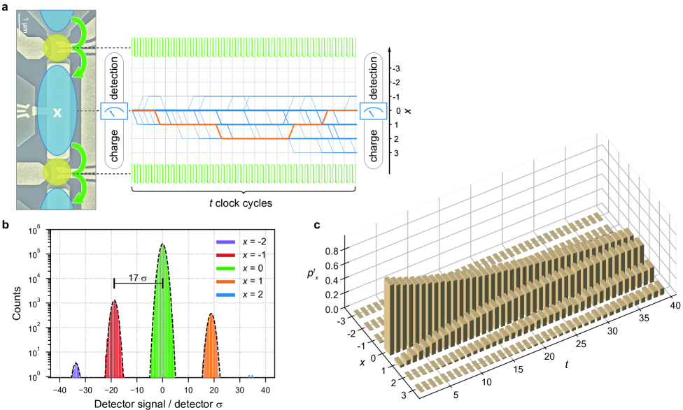
Figure 1: (a) Sample micrograph and measurement scheme. After the initial charge measurement $t$ clock cycles are applied. The paths taken by 30 simulated walkers (using error rates extracted from the counting statistics) are represented by blue lines, transitioning every clock cycle in $x$ by a step of $-1,0,+1$. The frequency with which each branch is visited is indicated by the linewidth. A final charge measurement yields the end-point of the random walk as the difference between initial and final charge. The orange line exemplifies a single random walk with self-intersections. (b) Signal to noise ratio: a (typical) histogram of the differential charge detection signal with the identified difference in electron number indicated by color. The peak separation is shown in units of the Gaussian noise amplitude $\sigma$ (black dashed lines indicate the corresponding Gaussian fits). (c) Measured statistics of finding the walker at position $x$ after $t$ steps.

Experimentally, the high-fidelity circuit for electron transfer is realized by a chain of quantum dots in which the first and the last dot are operated as single-electron pumps Kaestner2015 and the central dot provides the error signal as shown in Figure 1. A clock of frequency ($f=$ $30\text{\,}\mathrm{MHz}300\text{\,}\mathrm{MHz}$) drives the pumps to transfer one electron per cycle through the chain (from top to bottom in Figure 1).

Within one clock-cycle, the entrance barrier to the dynamic quantum dot is lowered and raised by the pump stimulus, isolating one electron from the source reservoir and then ejecting it over the high exit barrier; barrier height asymmetry between entrance and exit defines the transfer direction Kaestner2008 . The operating points of the pumps are chosen to minimize and approximately balance the error probabilities of transferring either zero or two electrons instead of one (with a slight bias towards zero-electron transfers, as this error rate only increases exponentially and not double-exponentially with deviations from the optimal operating point Kashcheyevs2010 ). The working points of the pumps are not retuned when operating the full circuit. Reproducible formation of quantum dots Gerster2018 allows to demonstrate high-fidelity operation of the circuit event at zero magnetic field, at which readout precision is enhanced by cryogenic reflectometry.

The excess charge $x$ from accumulating errors is inferred from a differential measurement by a charge detector capacitively coupled to the central dot, reading out the detector state before and after each sequence transferring $t$ electrons. As tunneling events are only enabled by the clocked stimulus applied to the pumps, a long detector integration-time up to $1\text{\,}\mathrm{m}\mathrm{s}$ can be chosen for unambiguous identification of $x$ with a signal to noise ratio of 17 (Figure 1b). A full histogram of detector states before and after the transfer sequence allows to reconstruct the shape of the Coulomb blockade peak resonance utilized by the charge detector and provides rigorous classification thresholds for the identification of $x$. The sequence of electron transfer and charge detection is repeated with the repetition rate limited by the detector integration-time (up to $4\text{\,}\mathrm{kHz}$), until a set number of counts ($N=$$1\text{\times}{10}^{5}2\text{\times}{10}^{6}$) is accumulated. Any deviations not aligned with the measurement timing, such as instabilities in the charge detector, are readily recognized and discarded, while unintended charge transitions during the operation of the pump are counted and correctly identified as errors.

Although the individual accuracy of the active components can exceed metrological precision Giblin2019 , their simultaneous operation in a mesoscopic circuit Fricke2011 precludes the prediction of transfer fidelity from component-wise characterization due to interactions and cross-talk between the elements in the chain, exemplifying the need for circuit-level benchmarking. Experimental evidence for strong discord between component-wise and circuit-level characterization is given in Supplementary Note II.2.

Here we report the measurement results on two devices: device A introduces the methodology to resolve effects beyond statistical noise of independent error accumulation in a high-fidelity circuit, while device B demonstrates the effects of memory with increased repetition frequency. Both devices share very similar device geometries and parameters.

Figure 2a shows the counting statistics measured for device A at $f=$30\text{\,}\mathrm{M}\mathrm{H}\mathrm{z}$$ for $t$ up to $10^{4}$ compared to predictions of the baseline model. General trends expected from the random walk are evident: for short sequences, $t<1000\ll(P_{+}\,P_{-})^{-1/2}$, the power-law rise of the probabilities $p^{t}_{|x|>0}$ corresponds to the exponential decay of error-free transfer fidelity $p^{t}_{0}$ which remains close to $1$. For longer sequences the distribution spreads and the weight of self-intersecting paths (e.g. orange line in Fig. 1) increases, in accordance with Eq. (1).

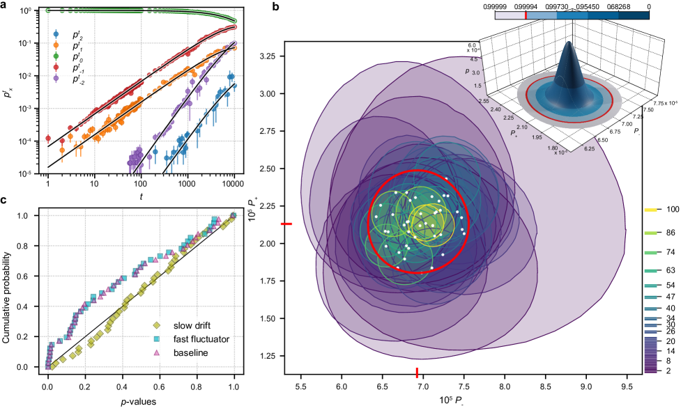
Figure 2: (a) Measured $p^{t}_{x}$ for device A; error bars are given by the standard deviation of the binomial distribution, solid lines show a least-squares fit of Eq. (1). (b) Likelihood-maximising $P_{\pm}$ (white dots) and $p>0.05$ consistency regions estimated separately for each sequence length (coded by color). The inset shows the probability density function of the Dirichlet distribution with parameter $\boldsymbol{\alpha}=($2.427\,195\text{\times}{10}^{3}3.504\,960\text{\times}{10}^{7}7.468\,530\text{\times}{10}^{2}$)$. The corresponding global best-fit values for $P_{\pm}$ are marked by red lines on the axes of the consistency-region plot. The color scale indicates the level of confidence at different coverage factors $k$ for a symmetric normal distribution; the red circle in both plots and the marker in the color scale indicates the region corresponding to $k=4$. (c) Empirical cumulative distribution of $p$-values for different models in comparison to the uniform distribution (black line).

The key question for random-walk benchmarking is whether the uncorrelated residual randomness defined by two probabilities $P_{+}$ and $P_{-}$ predicts the entire probability distribution. This question is answered in three steps: (i) significance testing of deviations from the baseline model as a statistical null hypothesis to delineate the inevitable sampling error from model error; (ii) extending the model to accommodate correlated excess noise Mavadia2018 detected in the first step; (iii) perform parameter estimation of the noise model that yields average values of $P_{\pm}$ with an estimate of the variability.

For consistency testing, we have increased the number $N$ of samples per sequence by a factor of $\sim 10$, and limited $t$ to 100. Fisherian significance tests Christensen2005 are used to define consistency regions of $p$-value greater than $0.05$ in the parameter space $(P_{+},P_{-})$ where the baseline model cannot be rejected at this significance level (see Methods). Figure 2b shows quasielliptic consistency regions computed for each sequence length $t$ separately, randomly clustering in a tight area with the sizes shrinking roughly as $\sim 1/\sqrt{t}$, as expected. Their overlap is only partial: best-fit global $(P_{+},P_{-})$ estimated from maximal likelihood (marked on the axes of Figure 2b) lies outside of $7$ regions out of $42$. A more rigorous test on whether this inconsistency can be explained by sampling error alone is provided by Fisher’s meta-analysis method (Figure 2c): under the null-hypothesis, the cumulative distribution of $p$-values obtained separately for each sequence length $t$ should be uniform (a straight line) Borenstein2009 ; Fisher1932 (see Supplementary Note III.3) which is not the case for the best-fit baseline model (triangles in Figure 2c). Quantitatively, the baseline model yields global Fisher’s combined $p<3\times 10^{-6}$, and hence is statistically rejected. We attribute this incompatibility to excess noise due to imperfections in the physical realization of the baseline model. Nevertheless, the partial overlap and the tight clustering observed in Figure 2b suggests that the excess noise is rather small. We model the excess noise as stochastic variability of $P_{\pm}$, and check whether it can be plausibly explained by the presence of two-level fluctuators Paladino2014 .

To quantify the excess noise, the model is now extended (part (ii) of the outline above) by drawing the step probabilities $P_{\pm}$ randomly from a Dirichlet distribution Ng2011 ; Johnson97 (Supplementary Note IV) over the standard 2-simplex; the corresponding parameters $\boldsymbol{\alpha}=\left\{\alpha\,\left\langle P_{-}\right\rangle,\alpha\,(1-\left\langle P_{+}\right\rangle-\left\langle P_{-}\right\rangle),\alpha\,\left\langle P_{+}\right\rangle\right\}$ are specified by two means, $\langle P_{\pm}\rangle$, and one additional concentration parameter $\alpha$ which controls the variance, $\Delta P_{\pm}^{2}=\left\langle P_{\pm}\right\rangle(1-\left\langle P_{\pm}\right\rangle)/(\alpha+1)$. The Dirichlet distribution is strongly peaked near the mean point for $\alpha\gg\left\langle P_{\pm}\right\rangle^{-1}$, and always guarantees $0\leq P_{\pm}\leq 1$. This extra randomness can be introduced at different timescales Ball2016 . Uncorrelated noise (new $P_{\pm}$ after each step of a walk) is equivalent to the baseline model with $P_{\pm}\to\left\langle P_{\pm}\right\rangle$, and is already ruled out by the significance tests above. We compare a “fast fluctuator” model in which a new pair of $P_{\pm}$ is drawn independently after completion of each individual random walk versus a “slow drift” model in which the values of $P_{\pm}$ are randomly reset only after all $N$ realizations for a fixed number of steps have been collected (precise excess noise model definitions are given in Supplementary Note IV.1 and IV.2, and the data acquisition timeline is illustrated in Fig. S1). Although short of proper time-resolved noise metrology OMalley2015 , contrasting these two correlated-noise models gives an indication of the relevant timescales (nanoseconds versus half-hour in the experiments). The sensitivity of Fisher’s significance testing makes it possible to distinguish between the two models, which cannot be resolved by the second moment of $\langle p_{x}^{t}\rangle$ as utilized, e.g., for noise-averaged fidelities in randomized benchmarking of quantum gates Mavadia2018 . The results of Fisher’s combined test (see Figure 2c) favour the “slow drift” ($p=0.71$) over the “fast fluctuator” ($p<3\times 10^{-6}$) model. The corresponding best-fitting Dirichlet distribution (parameters indicated by red lines on the axes of Figure 2b and plotted in the inset) gives $1\,\sigma$ uncertainty estimates $P_{-}=(6.92\pm 0.14)\times 10^{-5}$ and $P_{+}=(2.13\pm 0.08)\times 10^{-5}$. Parametric instability at only a few-percent level validates a suitably extended random walk model as a robust representation of error accumulation in this high-fidelity single-electron circuit.

In order to gain insight into a possible physics mechanism for excess noise and illustrate the robustness of statistical methods, we have simulated the experimental timeline using a random walk model with $P_{\pm}$ parameters subjected to $1/f$ noise from an ensemble of independent two-level fluctuators (see Supplementary Note V). The results follow the general pattern outlined above: (i) for a fixed size of the statistical sample, there is a threshold in the excess noise amplitude above which the data contradict both the baseline and the fast-fluctuator models but remain consistent with the slow-drift model. This threshold corresponds to excess noise sufficiently affecting probabilities of multiple errors per burst to reveal inconsistency with Eq. (1) in the tails ($|x|>1$) of the error syndrome distribution $p_{x}^{t}$. (ii) The estimated best-fit $\Delta P_{\pm}$ parameters correlate well with the standard deviation of the $P_{\pm}$ in the underlying simulation. (iii) Even a single fluctuator with a fixed switching rate (bimodal distribution of $P_{\pm}$ and a Poisson distribution of switching times Jenei2019 ) can generate detectable excess noise still consistent with our Dirichlet-based statistical models. As for the physics of the real device in a noisy environment, the simulations favor an explanation of the detected excess noise by the presence of multiple charge fluctuators over a single two-level system due to the absence of a bimodal signature in Fig. 2b. In conclusion, accurate statistics of error counts can give enough sensitivity to reliably estimate the baseline error rates $P_{\pm}$ and even capture a fingerprint of long-time correlations in the environment.

The methodology to quantify independent error accumulation described above makes it possible to probe the effect of increased clock frequency on the circuit and thereby investigate response times of the electron shuttle and interactions between subsequent steps. In device B the error rates are $P_{-}=(6.31\pm 0.23)\times 10^{-3}$ and $P_{+}=(2.71\pm 0.043)\times 10^{-2}$ at the same frequency of $30\text{\,}\mathrm{M}\mathrm{H}\mathrm{z}$ as device A investigated above. Ten-fold increase of the clock frequency to $300\text{\,}\mathrm{M}\mathrm{H}\mathrm{z}$ is introduced by uniform time compression of signals controlling the transfer operations; the resulting counting statistics is presented in Figure 3a (circles). The random-walk model with constant $P_{\pm}$, described by Eq. (1), no longer applies even qualitatively, which raises the question whether the fidelity of the circuit has decreased to a point where errors can no longer be considered rare as outlined in the beginning. This question is answered in the negative with the help of the following theorem defining a spread condition, which sets a precise bound on the applicability of the random-walk approach with possibly non-stationary error rates: If distributions $(p_{x}^{t})$ and $(p_{x}^{t+1})$ satisfy

$$\sum\limits_{y=-\infty}^{x-1}p_{y}^{t}\leq\sum\limits_{y=-\infty}^{x}p_{y}^{t+1}\leq\sum\limits_{y=-\infty}^{x+1}p_{y}^{t}\quad\text{for all }x,$$ (2)

then there exists a set of transition probabilities $P_{\pm 1}^{(x,t)}$ such that $(p_{x}^{t+1})$ is generated from $(p_{x}^{t})$ by a Markov chain $p_{x}^{t+1}=p_{x}^{t}+\sum_{s=\pm 1}\left[P_{s}^{(x-s,t)}p_{x-s}^{t}-P_{s}^{(x,t)}p_{x}^{t}\right]$. Conversely, any discrete-space, discrete-time random walk with steps of lengths at most $1$ (our definition of a high-fidelity circuit) satisfies the spread condition (2), see Supplementary Note VII for proof of both claims.

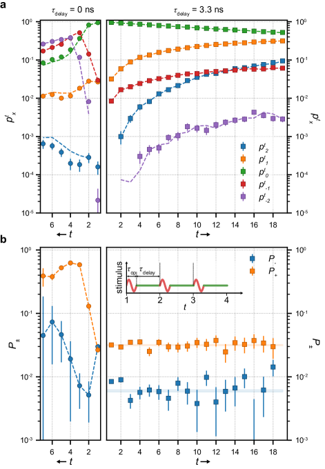
Figure 3: (a) Measured $p^{t}_{x}$ for device B at a clock frequency of $300\text{\,}\mathrm{MHz}$ and $\tau_{\text{Delay}}=$0\text{\,}\mathrm{s}$$ (left, $t$-axis inverted) and $\tau_{\text{Delay}}=$3.\overline{3}\text{\,}\mathrm{ns}$$ (right). Dashed lines represent $p_{x}^{t}$ predicted by deconvolved single-step error rates and $p^{t-1}_{x}$. (b) Single-step error rates $P_{\pm}^{t}$ for $\tau_{\text{Delay}}=$0\text{\,}\mathrm{s}$$ (left, $t$-axis inverted, dashed lines show guide to the eye) and $\tau_{\text{Delay}}=$3.\overline{3}\text{\,}\mathrm{ns}$$ (right, translucent area corresponds to the $1\,\sigma$ uncertainty estimates). Inset depicts the timing diagram of the sequence – a stimulus of duration $\tau_{\text{op}}$ drives the transfer operation followed by delay time $\tau_{\text{Delay}}$ before the next step.

We find that the distributions measured on device B do satisfy the spread condition (2) as long as all $x$ are fully resolved in counting ($t\leq 6$). We estimate the non-stationary but $x$-homogeneous single-step error probabilities of the corresponding Markov chains, $P_{\pm 1}^{(x,t)}=P_{\pm}^{t}$, by a numerical deconvolution of the Markov process equation (Supplementary Note II.1). The resulting error rates $P_{\pm}^{t}$ in Fig. 3b provide reasonable prediction (dashed lines) of the measured $p_{x}^{t}$ in Fig. 3a (circles). The $t$-dependence of $P_{\pm}^{t}$ is strong and reproduced well above the noise. This implies memory: probabilities for the next step depend on how many steps have taken place before. $P_{\pm}^{t}$ do not saturate within $t\leq 6$ indicating a long memory time of more than $6\,\tau_{\text{op}}=$20\text{\,}\mathrm{n}\mathrm{s}$$.

To probe this memory effect, we introduce a delay time $\tau_{\mathrm{Delay}}$ between otherwise unaltered signals driving the transfer operations thus extending the physical time $f^{-1}$ corresponding to a single step of the random walk from $\tau_{\text{op}}$ to $\tau_{\text{op}}+\tau_{\text{Delay}}$ as sketched in Figure 3b. With increasing delay, a gradual reduction of the $t$-dependence in $P_{\pm}^{t}$ is observed until, for $\tau_{\mathrm{Delay}}>$3\text{\,}\mathrm{ns}$$ (see right part of Fig. 3a and b), the stationary behaviour consistent with the baseline model is recovered. Surprisingly, $\tau_{\text{Delay}}$ sufficient to recover stationary behaviour is on the order of a single step duration $\tau_{\text{op}}$, significantly shorter than the number of steps with pronounced memory effect at $\tau_{\text{Delay}}=$0\text{\,}\mathrm{ns}$$ (Figure 3b). Both times are significantly longer than the expected timescales in GaAs systems for relaxation via electron-electron or phonon interaction Ridley1991 ; Snoke1992 ; Molenkamp1992 , and raise the need for a dedicated investigation. In Fig. 3b $P^{t}_{\pm}$, estimated at each $t$ by deconvolution (squares), are compared with the confidence intervals of the “slow-drift” model with stationary $P_{\pm}$ (color bands). The comparison shows good agreement and is consistent with our framework for random-walk benchmarking of high-fidelity single-electron circuits. For the showcased device, circuit-level interactions and memory effects significantly lower the attainable clock speed compared to record frequencies for individual pumps reported in the literature Yamahata2016 . However, benchmarking by error accumulation introduces a tool to investigate these limitations and identify possible mitigation-techniques since $\tau_{\text{op}}$ and $\tau_{\text{Delay}}$ can be freely adjusted with error rates still accurately estimated on the circuit level, as long as these remain within the high-fidelity bound monitored by the spread condition.

In conclusion, the view of single-electron components as elements of a digital circuit has enabled an abstract and universal description of fidelity in terms of the random walk of an error syndrome. Accumulation of errors over long sequences allows to probe fast and accurate operations beyond the bandwidth of a slow single-charge detector. The accompanying statistical methodology quantifies the stability of the error process and uncovers short memory times, both of which are elusive to direct observation. In quantum metrology, an accurate estimate of the circuit error has an immediate application: the variance of the current $I=(I_{s}+I_{d})/2$ flowing into ($I_{s}$) and out of ($I_{d}$) the circuit is given by the variance of the differential charge $x$, which corresponds to the displacement current $I_{s}-I_{d}=efx/t$. Hence, the variance of $x$, $\Delta x^{2}\approx(\langle P_{+}\rangle+\langle P_{-}\rangle)\,t+(\Delta P_{+}^{2}+\Delta P_{-}^{2})\,t^{2}$, provides a bound for the deviation of the current $I$ from the error-free value $ef$, enabling counting-verification of a primary standard for the ampere. In the broader context, sensitive tests of single-electron circuits create new ground for developing benchmarking techniques of engineered quantum systems.

Methods

Devices A and B were fabricated from GaAs/AlGaAs heterostructures with two dimensional electron gas (2DEG) nominally $90\text{\,}\mathrm{n}\mathrm{m}$ below the surface. Quantum dots are formed by CrAu top gates depleting a shallow-etched mesa Gerster2018 . The charge detector is formed against the edge of a separate mesa and capacitively coupled to the central quantum dot via a floating gate Fricke2014 . All measurements were performed in a dilution refrigerator at a base temperature of $20\text{\,}\mathrm{mK}$ and $0\text{\,}\mathrm{T}$ external field. The charge detector signal is read out by rf reflectometry Schoelkopf1998 . Sinusoidal pulses generated by arbitrary waveform generators modulate the entrance barriers of the single electron pumps and drive the clock-controlled electron transfer Kaestner2015 . The drift-stability due to control voltages is estimated to be better than $10^{-8}$. Charge transfer and detector readout are triggered in a sequence: (i) readout of the initial detector state, (ii) application of $t$ sinusoidal pulses to both pumps simultaneously, (iii) readout of the final detector state, (iv) reset by connecting the intermediate dot to source. The difference between initial and final detector state yields the charge $x$ deposited on the central quantum dot by the burst transfer, providing raw data for subsequent statistical analysis. Fisher’s $p$-value for each experimentally measured $x$-resolved set of $N$ counts is defined as the probability of an equally or more extreme outcome under the null-hypothesis being tested (either the baseline random walk or one of the two excess noise models with Dirichlet-distributed $P_{\pm}$); it is evaluated by Monte Carlo sampling as described in the Supplementary Notes III and IV.

Supplemental information

Contents

1. I Baseline model
2. II Assessing $P_{\pm}$ values from the experimental data
   1. II.1 Estimation of step-wise probabilities $P_{\pm}^{t}$ by deconvolution
   2. II.2 Comparison between measured and predicted $P_{\pm}$
3. III Model consistency testing
   1. III.1 Fisher’s significance testing
   2. III.2 Consistency regions
   3. III.3 Combining the $p$-values
   4. III.4 Maximum likelihood estimation
4. IV Dirichlet distribution-based random-walk models
   1. IV.1 Model 1 (fast fluctuator)
      1. Model description
      2. Probability mass function
      3. Consistency testing
   2. IV.2 Model 2 (slow drift)
      1. Model description
      2. Probability mass function
      3. Consistency testing
5. V Excess noise simulations
   1. V.1 Noise simulation procedure
   2. V.2 Noise simulation results
      1. Detection of excess noise
      2. Example of statistical methodology applied to the simulated data
      3. Simulations of a single fluctuator
6. VI Slow drift model: variance of random walker’s position
7. VII Proof for spread condition

I Baseline model

Consider a time-homogeneous discrete-time random walk on the set of integers which starts at 0 and at each step moves $+1$ with probability $P_{+}$, moves $-1$ with probability $P_{-}$ and stays at the same vertex with probability $P_{0}$; here we assume $P_{+},P_{-},P_{0}\in(0,1)$, $P_{-}+P_{0}+P_{+}=1$.

To describe this process formally, consider a random variable $\mathbf{K}=(K_{-1},K_{0},K_{+1})$ following a multinomial distribution with $t>0$ trials and three categories, with associated probabilities $P_{-}$, $P_{0}$ and $P_{+}$, respectively. Then the random variable $X=K_{+1}-K_{-1}$ corresponds to the position of the random walker after $t$ steps, since all steps can be modeled with independent discrete random variables with three possible outcomes ($-1$, $0$ and $+1$, respectively) and respective probabilities $P_{-}$, $P_{0}$ and $P_{+}$. First we show that the probability mass function of the discrete variable $X\in\{-t,-t+1,\ldots,t-1,t\}$ is given by (1) in the main text; i.e., let ${p_{x}^{t}}:=\Pr(X=x)$, then

Claim 1.

The probability mass function (PMF) of the variable $X$ is

$${p_{x}^{t}}=\begin{cases}(P_{+})^{x}(P_{0})^{t-x}\,\binom{t}{x}\,{}_{2}F_{1}\left(\frac{x-t}{2},\frac{x-t+1}{2};x+1;\frac{4P_{+}P_{-}}{P_{0}^{2}}\right),&x\geq 0,\\ (P_{-})^{-x}(P_{0})^{t+x}\,\binom{t}{-x}\,{}_{2}F_{1}\left(\frac{-x-t}{2},\frac{-x-t+1}{2};-x+1;\frac{4P_{+}P_{-}}{P_{0}^{2}}\right),&x<0,\end{cases}$$ (3)

for $x\in\{-t,-t+1,\ldots,t-1,t\}$.

Proof.

Suppose that $x\geq 0$; then the event $X=x$, i.e., the event of the random walker being at the position $x$ after $t$ steps, is equivalent to the event that the multinomially distributed variable $\mathbf{K}=(K_{-1},K_{0},K_{+1})$ satisfies $K_{+1}-K_{-1}=x$ (i.e., to the event that the random walker has moved $K_{+1}$ steps to the right and $K_{-1}=K_{+1}-x$ steps to the left). Therefore $\Pr(X=x)$ can be obtained from the multinomial distribution’s PMF as

$$\Pr(X=x)=\sum_{\begin{subarray}{c}\mathbf{k}:\\ k_{1}-k_{-1}=x\\ k_{-1}+k_{0}+k_{1}=t\end{subarray}}\Pr(\mathbf{K}=\mathbf{k}).$$

Since $\mathbf{K}$ follows a multinomial distribution with $t>0$ trials and three categories with respective probabilities $P_{-}$, $P_{0}$ and $P_{+}$, its PMF is given by

$$\Pr(\mathbf{K}=\mathbf{k})=\frac{t!}{k_{-1}!k_{0}!k_{1}!}\,P_{-}^{k_{-1}}P_{0}^{k_{0}}P_{+}^{k_{1}},$$

where $\mathbf{k}:=(k_{-1},k_{0},k_{1})$ is a vector of nonnegative integers satisfying $k_{-1}+k_{0}+k_{1}=t$.

Notice that such $\mathbf{k}$ can additionally satisfy $k_{1}-k_{-1}=x\geq 0$ only if $\mathbf{k}$ is of the form $\mathbf{k}=(s,t-x-2s,x+s)$, for some nonnegative integer $s$. Moreover, since $k_{0}\geq 0$, we obtain the constraint $t-x-2s\geq 0$, i.e., $s\leq 0.5(t-x)$. We conclude that all suitable vectors $\mathbf{k}$ are parametrized by a nonnegative integer $s$, which is upper-bounded by $0.5(t-x)$ (more precisely, the maximal valid $s$ value is the floor function of $0.5(t-x)$). For each such $s$ the corresponding vector is $\mathbf{k}=(s,t-x-2s,x+s)$ and the probability of the event $\mathbf{K}=\mathbf{k}$ is

$$\Pr(\mathbf{K}=(s,t-x-2s,x+s))=\frac{t!}{s!(x+s)!(t-x-2s)!}\,P_{-}^{s}P_{0}^{t-x-2s}P_{+}^{x+s},$$

respectively. Thus $p_{x}^{t}:=\Pr(X=x)$ is simply the sum of these multinomial probabilities:

$$p_{x}^{t} =\sum_{\begin{subarray}{c}\mathbf{k}:\\ k_{1}-k_{-1}=x\\ k_{-1}+k_{0}+k_{1}=t\end{subarray}}\Pr(\mathbf{K}=\mathbf{k})=\sum_{s=0}^{(t-x)/2}\Pr\left(\mathbf{K}=(s,t-x-2s,x+s)\right)$$

$$=\sum_{s=0}^{(t-x)/2}\frac{t!}{s!(x+s)!(t-x-2s)!}\,P_{-}^{s}P_{0}^{t-x-2s}P_{+}^{x+s}.$$

The latter quantity can be equivalently expressed as

$$p_{x}^{t} =P_{+}^{x}P_{0}^{t-x}\,\binom{t}{x}\sum_{s=0}^{(t-x)/2}\frac{(t-x)!}{(x+s)!(t-x-2s)!s!}\,\left(\frac{P_{+}P_{-}}{P_{0}^{2}}\right)^{s}.$$

Let us show that

$$\sum_{s=0}^{(t-x)/2}\frac{(t-x)!}{(x+s)!(t-x-2s)!s!}\,\left(\frac{P_{+}P_{-}}{P_{0}^{2}}\right)^{s}=\,{}_{2}F_{1}\left(\frac{x-t}{2},\frac{x-t+1}{2};x+1;\frac{4P_{+}P_{-}}{P_{0}^{2}}\right),$$ (4)

which will establish (3) and conclude the proof.

We start by rewriting the LHS of (4). Observe that $(x+s)!=(x+1)_{s}$, where $(a)_{s}:=a(a+1)\ldots(a+s-1)$ stands for the Pochhammer’s symbol. Furthermore,

$$\frac{(t-x)!}{(t-x-2s)!} =(t-x)(t-x-1)\ldots(t-x+1-2s)$$

$$=4^{s}\left(\frac{t-x}{2}-s+1\right)_{s}\left(\frac{t-x-1}{2}-s+1\right)_{s}$$

$$=4^{s}\left(\frac{x-t}{2}\right)_{s}\left(\frac{x-t+1}{2}\right)_{s},$$

where the last step applies the identity $(-a)_{s}=(-1)^{s}(a-s+1)_{s}$. Therefore

$$\sum_{s=0}^{(t-x)/2}\frac{(t-x)!}{(x+s)!(t-x-2s)!s!}\,\left(\frac{P_{+}P_{-}}{P_{0}^{2}}\right)^{s}=\sum_{s=0}^{(t-x)/2}\frac{\left(\frac{x-t}{2}\right)_{s}\left(\frac{x-t+1}{2}\right)_{s}}{(x+1)_{s}\,s!}\,\left(\frac{4P_{+}P_{-}}{P_{0}^{2}}\right)^{s}.$$

The upper limit $(t-x)/2$ in the latter sum can be replaced with infinity, since the numerator $\left(\frac{x-t}{2}\right)_{s}\left(\frac{x-t+1}{2}\right)_{s}$ is zero for the additional terms with $s>0.5(t-x)$. It remains to recognize now that the sum coincides with the definition of the Gaussian hypergeometric function ${}_{2}F_{1}$. We have verified (4), which concludes the proof of (3) when $x\geq 0$. The case $x<0$ follows from similar considerations. ∎

We note that discrete distributions similar to $X$ have been considered before. In particular, Zhang2011 considers an analogue of our random variable $X$ and computes $p_{0}^{t}$ (termed “return probability $p_{0}(t)$” in the paper). $X$ is also closely related to the inverse trinomial distribution shimizu1991 ; Aoyama05 , defined via a random walk on the line. Nevertheless, we are not aware of prior work establishing the PMF (3) of $X$.

The return probability for the random walk, $p_{0}^{t}$, is the probability of error-free electron transfer in the context of our benchmarking application, and hence can also be interpreted as transfer fidelity. As long as the contribution of the return paths is negligible, $p_{0}^{t}$ decays exponentially, but for larger $t$ the exponential decay is modified. Below we derive an explicit asymptotics that characterizes both sides of this crossover.

Claim 2.

$$p_{0}^{t}\approx\begin{cases}P_{0}^{t}\,,&t\ll(P_{+}{P_{-}})^{-1/2}\\ \frac{\left(P_{0}+2\sqrt{P_{+}P_{-}}\right)^{1/2+t}}{(4\pi\,t)^{1/2}(P_{+}\,P_{-})^{1/4}}\,,&t\gg(P_{+}{P_{-}})^{-1/2}\end{cases}.$$

Proof.

By (3) we have

$$p_{0}^{t}=(P_{0})^{t}{}_{2}F_{1}\left(\frac{-t}{2},\frac{-t+1}{2};1;z\right),$$

where we denote $z=4P_{+}P_{-}/P_{0}^{2}$. We start by observing that by a quadratic transformation (DLMF, , Eq. 15.8.13) we have

$${}_{2}F_{1}\left(\frac{-t}{2},\frac{-t+1}{2};1;z\right)={}_{2}F_{1}\left(-t,0.5;1;\zeta\right)\cdot\left(1-0.5\zeta\right)^{-t},$$ (5)

where the variable $\zeta$ is defined by $\frac{\zeta}{2-\zeta}=\sqrt{z}$, i.e.,

$$\zeta=\frac{2\sqrt{z}}{1+\sqrt{z}}=\frac{4\sqrt{P_{+}P_{-}}}{P_{0}+2\sqrt{P_{+}P_{-}}}\quad\text{and}\quad(1-0.5\zeta)^{-1}=\frac{P_{0}+2\sqrt{P_{+}P_{-}}}{P_{0}}.$$

Using the equality (5) we arrive at

$$p_{0}^{t}=(P_{0}+2\sqrt{P_{+}P_{-}})^{t}\,{}_{2}F_{1}\left(-t,0.5;1;\zeta\right).$$ (6)

Since the hypergeometric function on the right hand side of (6) is a degree-$t$ polynomial in the variable $\zeta\ll 1$, for small values of $t$ we can approximate

$$P_{0}+2\sqrt{P_{+}P_{-}}\approx P_{0}\quad\text{and}\quad{}_{2}F_{1}\left(-t,0.5;1;\zeta\right)\approx 1,$$

leading to the first part of the claim.

Now we consider (6) with fixed $\zeta$ when $t\to+\infty$. We apply an asymptotic expansion of the hypergeometric function in case of a large argument due to Erdélyi (Erdelyi53, , p. 77, Eq. 15), which exploits the relation between the (Gaussian) hypergeometric function ${}_{2}F_{1}$ and the confluent hypergeometric function ${}_{1}F_{1}$:

$${}_{2}F_{1}\left(-t,0.5;1;\zeta\right)\sim_{1}F_{1}(0.5;1;-t\zeta)\sim\frac{\Gamma(1)(t\zeta)^{-0.5}}{\Gamma(0.5)}\left(1+O\left(\left|t\zeta\right|^{-1}\right)\right)\sim\frac{1}{\sqrt{\pi t\zeta}}.$$

Combining this with (6) and substituting $\zeta=\frac{4\sqrt{P_{+}P_{-}}}{P_{0}+2\sqrt{P_{+}P_{-}}}$ gives us the second part of the claim. ∎

Finally, consider $N$ independent observations of the random variable $X$, i.e., i.i.d. random variables $X_{1},\ldots,X_{N}\sim X$. Let $Z_{x}=\left|\left\{j\in\{1,\ldots,N\}\;:\;X_{j}=x\right\}\right|$ be the number of times the value $x\in\{-t,\ldots,t\}$ appears among these $N$ observations. Then the random variable

$$\mathbf{Z}_{N,t}=(Z_{-t},Z_{-t+1},\ldots,Z_{0},Z_{1},\ldots,Z_{t})$$

follows a multinomial distribution with $N$ trials and $2\,t+1$ categories, labeled from $-t$ to $t$, and respective probabilities ${p_{x}^{t}}$. When there is no ambiguity, this notation is simplified to $\mathbf{Z}$. The probability to observe a particular vector $\mathbf{z}\in\mathbb{N}_{0}^{2t+1}$, $\sum_{x=-t}^{t}z_{x}=N$ (where $\mathbb{N}_{0}$ stands for the set of nonnegative integers) is

$$\Pr(\mathbf{Z}=\mathbf{z})=N!\prod_{x=-n}^{n}\frac{\left(p_{x}^{t}\right)^{z_{x}}}{z_{x}!}.$$ (7)

II Assessing $P_{\pm}$ values from the experimental data

II.1 Estimation of step-wise probabilities $P_{\pm}^{t}$ by deconvolution

Under the assumption that the $P_{\pm}^{t}$-values are independent of the position $x$ of the random walker, they can be extracted by deconvolution of $p_{x}^{t}$ and $p_{x}^{t+1}$. For that let us expand the model used so far and consider a random walk on the set of integers which at time $t$ performs transition $x\mapsto x+j$ with probability $P_{j}^{t}$, $x,j\in\mathbb{Z}$. Here $P_{j}^{t}\in(0,1)$ for all $j$ and $\sum_{j\in\mathbb{Z}}P_{j}^{t}=1$.

The experiment yields two vectors from $\mathbb{R}^{2m+1}$, $m\in\mathbb{N}$, representing the distributions $\mathbf{p}^{t}=\left(p_{-m}^{t},\ldots,p_{-1}^{t},p_{0}^{t},p_{1}^{t},\ldots,p_{m}^{t}\right)$ and $\mathbf{p}^{t+1}=\left(p_{-m}^{t+1},\ldots,p_{-1}^{t+1},p_{0}^{t+1},p_{1}^{t+1},\ldots,p_{m}^{t+1}\right)$. We shall assume $P_{j}^{t}=0$ for all $j\in\mathbb{Z}$ s.t. $\left|j\right|\geq m$. The distribution $\mathbf{p}^{t+1}$ represents the position of the random walker after $t+1$ steps and satisfies

$$p_{x}^{t+1}=\sum_{j\in\mathbb{Z}}P_{j}^{t}p_{x-j}^{t},$$

i.e., $\mathbf{p}^{t+1}=\mathbf{P}^{t}\ast\mathbf{p}^{t}$ is the discrete convolution of $\mathbf{P}^{t}=\left(P_{-m}^{t},\ldots,P_{-1}^{t},P_{0}^{t},P_{1}^{t},\ldots,P_{m}^{t}\right)$ and $\mathbf{p}^{t}$. Therefore $\mathbf{P}^{t}$ can be extracted by discrete deconvolution, which is performed as follows.

Let $\mathfrak{p}^{t+1}$, $\mathfrak{p}^{t}$ and $\mathfrak{P}^{t}$ stand for the Fourier transform of $\mathbf{p}^{t+1}$, $\mathbf{p}^{t}$ and $\mathbf{P}^{t}$, respectively, then

$$\mathfrak{p}^{t+1}={\mathfrak{P}^{t}}\cdot\mathfrak{p}^{t},\quad\text{i.e.,}\quad\mathfrak{P}^{t}_{x}=\frac{\mathfrak{p}^{t+1}_{x}}{\mathfrak{p}^{t}_{x}}\quad\text{for all }x.$$

The vector $\mathfrak{p}^{t}$ is calculated from $p^{t}$ as

$$\mathfrak{p}_{x}^{t}=\sum_{n=-m}^{m}p_{n}^{t}\exp{\left(-\mathrm{i}x\beta_{n}\right)},\quad\text{where }\mathrm{i}=\sqrt{-1}\text{ and }\beta_{n}=\frac{2\pi n}{2m+1},$$

similarly for $\mathfrak{p}^{t+1}$. Now we can the get $\mathbf{P}^{t}$ by applying the inverse discrete Fourier transform to $\mathfrak{P}^{t}$:

$$P_{j}^{t}=\frac{1}{2m+1}\sum_{n=-m}^{m}\mathfrak{P}^{t}_{n}\exp{\left(\mathrm{i}n\beta_{j}\right)}.$$

Further details on how the deconvolution is performed and the uncertainty propagates can be found in Eichstaedt2016 . Now that we have extracted $\mathbf{P}^{t}$, we find for the experiment described in the main text, that $P_{|j|>1}^{t}\approx 0$ which allows us to approximate $P_{+}^{t}=P^{t}_{+1}$, and $P_{-}^{t}=P^{t}_{-1}$.

II.2 Comparison between measured and predicted $P_{\pm}$

The characterization of the single electron pumps gives us their transport statistic $q_{m}^{(i)}$, which is the probability of pump $i\in\left\{1,2\right\}$ transporting $m\in\mathbb{Z}$ electrons. Assuming independence of simultaneous pump operation we can calculate the probability $P_{x}$ that charge on the island increases by $x\in\mathbb{Z}$ electrons (here $P_{\pm 1}$ is equivalent to $P_{\pm}$ in (1) in the main text) as

$$P_{x}(\text{predicted})=\sum\limits_{m}q_{m+x}^{(1)}\cdot q_{m}^{(2)}\,.$$ (8)

Table S1 provides an example for agreement between measured and predicted values of $P_{\pm}$ for non-interacting pumps.

	single pumps
$m$	$q_{m}^{(1)}$	$q_{m}^{(2)}$
0	$0.000\,21$ p m 0.00005	$3.6$ p m 2.8 e-05
1	$0.999\,82$ p m 0.00006	$0.999\,975$ p m 0.000019
2	$0.0$ p m 2.0 e-05	$0.0$ p m 1.2 e-05

	whole device
$x$	$P_{x}$ (measured)	$P_{x}$ (predicted)
$-1$	$0.000\,12$ p m 0.00004	$0.000\,21$ p m 0.00005
$0$	$0.999\,78$ p m 0.00005	$0.999\,80$ p m 0.00006
$1$	$0.0$ p m 2.1 e-05	$3.6$ p m 3.4 e-05

Table S1: Comparison between measured and predicted values of $P_{x}$, showing good agreement.

For the measurement in Table S2 the waveform of the pump drive was changed from a low-frequency sinusoidal to a sharp voltage transient. Here we see a strong disagreement between the prediction of single pump characterization and the measurement of the $P_{\pm}$-values. This disagreement is caused by a strong shift of the operation point which occurs as soon as the pumps are operated simultaneously, indicating a strong correlation between the pumps.

	single pumps
$m$	$q_{m}^{(1)}$	$q_{m}^{(2)}$
0	$0.000\,12$ p m 0.00016	$0.000\,00$ p m 0.00014
1	$0.999\,74$ p m 0.00019	$1.000\,00$ p m 0.00014
2	$0.000\,12$ p m 0.00017	$0.000\,00$ p m 0.00014

	whole device
$x$	$P_{x}$ (measured)	$P_{x}$ (predicted)
-1	$0.239$ p m 0.006	$0.000\,12$ p m 0.00021
0	$0.776$ p m 0.005	$0.999\,74$ p m 0.00024
1	$0.000\,12$ p m 0.00016	$0.000\,12$ p m 0.00022

Table S2: Disagreement between measured and predicted $P_{x}$-values for sharp-transient waveform.

III Model consistency testing

The experimental data consist of observations (actually, rebinned observations as described in Supplementary Note III.2) of random variables $\mathbf{Z}_{N_{1},t_{1}}$, $\mathbf{Z}_{N_{2},t_{2}}$, …, $\mathbf{Z}_{N_{L},t_{L}}$, for several different pairs $(N_{1},t_{1})$, …, $(N_{L},t_{L})$, which, according to the model outlined in Supplementary Note I, all share the same step probabilities $(P_{-},P_{+})$.

We consider the problem of determining if there is a parameter $P_{\pm}$ such that the experimental data do not contradict the model, at the fixed significance level. More generally, we are interested in extracting a region in the parameter space such that the experimental data do not contradict the model for each choice of the parameter from the region; for brevity, we will refer to this region as consistency region. It should be stressed that this approach is different from parameter estimation problem, in that here we are interested in parameter values which cannot be statistically rejected as incompatible with the data, whereas the parameter estimation techniques deal with estimating the values of the parameters in some fashion, e.g., by finding the values of parameters under which the experimental data are most probable under the assumed model.

The problem of testing consistency of the model with a specific parameter value is twofold: since the data correspond to several pairs of $(N,t)$, with different parameters $N,t$ but the same step probabilities $(P_{-},P_{+})$, there are two questions to be asked:

1. Are the data for the particular value of $(N,t)$ consistent with the model for some parameter $P_{\pm}$?

2. Are all the data consistent with the model for some fixed value of $P_{\pm}$?

We start by testing consistency with the model in case of an observation of $\mathbf{Z}_{N,t}$ for a single pair $(N,t)$.

III.1 Fisher’s significance testing

Let $\mathbf{z}_{0}$ be an observation of the random variable $\mathbf{Z}:=\mathbf{Z}_{N,t}$, with prescribed parameters $t,N$ but unknown probabilities $P_{-},P_{0},P_{+}$.

We employ Fisher’s significance testing framework in order to extract the consistency regions for the parameter ${\boldsymbol{\theta}}=(P_{-},P_{0},P_{+})$. In its simplest form, a Fisherian test formulates Christensen2005 a single hypothesis, the null hypothesis $H_{0}$, which specifies the null distribution (i.e., in our case $H_{0}:{\boldsymbol{\theta}}={\boldsymbol{\theta}}^{*}$ for some fixed ${\boldsymbol{\theta}}^{*}$); then a certain test statistic $T$ is computed from the observation $\mathbf{z}_{0}$, leading to a value $T(\mathbf{z}_{0})$. The $p$-value of the test is the tail probability of $T(\mathbf{Z})$ under $H_{0}$. In our setting, the test statistic will be non-negative and smaller values will indicate stronger disagreement with the null hypothesis. Then the $p$-value of the test is

$$p(\mathbf{z}_{0})=\sum_{\begin{subarray}{c}\mathbf{z}:\\ T(\mathbf{z})\leq T(\mathbf{z}_{0})\end{subarray}}\Pr(\mathbf{Z}=\mathbf{z}),$$

where $\Pr(\mathbf{Z}=\mathbf{z})$ stands for the probability of the event $\mathbf{Z}=\mathbf{z}$ under the null hypothesis and the sum is over all those values $\mathbf{z}$ of the random vector $\mathbf{Z}$ that satisfy $T(\mathbf{z})\leq T(\mathbf{z}_{0})$ In the Fisher’s significance testing framework the $p$-value is interpreted as “a measure of extent to which the data do not contradict the model” (Christensen2005, , p.122). Therefore Fisher’s significance testing allows to check if $H_{0}$ must be rejected (at the chosen significance level) for the particular value $\boldsymbol{\theta}^{*}$; next, we shall employ Fisher’s significance testing to extract the region of those $\boldsymbol{\theta}$ values for which the respective $H_{0}$ cannot be rejected, see Supplementary Note III.2.

The problem of testing whether the parameters of a multinomial distribution equal specified values has been well-investigated Conover1972 ; Smith1981 ; Cressie1984 ; Jann2008 . The common approaches (such as Pearson’s $\chi^{2}$ test, $G^{2}$ test or power-divergence test Cressie1984 which subsumes the former tests) are asymptotic tests which can be highly biased. This is due to the fact that under the null hypothesis the random variable $X$ has vanishingly small tail probabilities (and the actual observed samples $\mathbf{z}$ have zero observed counts in the respective positions). This phenomenon makes the asymptotic tests ill-suited for the actual data.

An alternative to the aforementioned tests is the exact multinomial test Cressie1984 , which enumerates all possible multinomial outcomes; its test statistic $T$ is the probability of obtaining the particular outcome under the null hypothesis. Then the $p$-value of the test is

$$\sum_{\begin{subarray}{c}\mathbf{z}:\\ \Pr(\mathbf{Z}=\mathbf{z})\leq\Pr(\mathbf{Z}=\mathbf{z}_{0})\end{subarray}}\Pr(\mathbf{Z}=\mathbf{z}).$$

However, the exhaustive enumeration quickly becomes computationally intractable as $N$ grows. We instead apply a Monte Carlo test (proposed in Barnard1963 , see also Hope1968 ; Besag1992 ; Jann2008 ), which can be seen as an extension of the exact multinomial test. In the Monte Carlo hypothesis testing procedure, a large number (say, $N_{\mathrm{sim}}$) samples from the multinomial distribution under the null hypothesis are simulated; for each sample $\mathbf{z}$ the test statistic $\Pr(\mathbf{z})$ is calculated (i.e., the probability to draw $\mathbf{z}$ from the distribution $\mathbf{Z}$ under the null hypothesis). Let $k$ be the number of samples for which the test statistic is at least as extreme as for the observed vector $\mathbf{z}_{0}$ (i.e., the number of samples $\mathbf{z}$ for which $\Pr(\mathbf{z})\leq\Pr(\mathbf{z}_{0})$). Then the $p$-value of the test is $(k+1)/(N_{\mathrm{sim}}+1)$.

III.2 Consistency regions

Since $P_{0}=1-P_{+}-P_{-}$, the Monte Carlo tests are applied to extract $95\%$ consistency region for the pair $(P_{-},P_{+})$. This region is defined as the set of all admissible $(P_{-},P_{+})$ values for which the $p$-value obtained by testing the hypothesis $H_{0}:{\boldsymbol{\theta}}=(P_{-},(1-P_{-}-P_{+}),P_{+})$ is at least $0.05$.

In practice, since the observed vector $\mathbf{z}_{0}$ has many zero entries (as $N$ is too small to observe “$X=x$” when $\left|x\right|$ is large) and, since the experimental data is limited to small $\left|x\right|$, the data are rebinned. Depending on the dynamical range of the detector and available computational resources, we consider a random variable $\tilde{\mathbf{Z}}=(\tilde{Z}_{-3},\tilde{Z}_{-2},\tilde{Z}_{-1},\tilde{Z}_{0},\tilde{Z}_{1},\tilde{Z}_{2},\tilde{Z}_{3})$ instead of the random variable $\mathbf{Z}$ where

$$\tilde{Z}_{-3}=\sum_{x\leq-3}Z_{x},\quad\tilde{Z}_{3}=\sum_{x\geq 3}Z_{x},\text{ and }\tilde{Z}_{x}=Z_{x},\ \left|x\right|\leq 2,$$ (9)

and perform the aforementioned tests against an observation $\tilde{\mathbf{z}}_{0}$ of $\tilde{\mathbf{Z}}$. Further on, this subtlety will be assumed implicitly, i.e., when talking of the random variable $\mathbf{Z}$ or its observation $\mathbf{z}_{0}$, the rebinned counterparts $\tilde{\mathbf{Z}}$ and $\tilde{\mathbf{z}}_{0}$ are to be understood.

III.3 Combining the $p$-values

The discussion above attempts to answer if the data are consistent with some $P_{\pm}$, for a particular value of $(N,t)$; the challenge now is to combine the statistical tests done for all $L$ pairs of $(N,t)$. While for each fixed pair $\left(N,t\right)$ the $95\%$ consistency region can be constructed from the observation of the respective $\mathbf{Z}_{N,t}$, the goal is to obtain a global measure of discrepancy between the data and the hypothesis $H_{0}:{\boldsymbol{\theta}}=(P_{-},(1-P_{-}-P_{+}),P_{+})$, taking into account the observations for all pairs $(N,t)$.

This task can be viewed as the problem of combining several independent $p$-values, which arises in meta-analysis Borenstein2009 . When testing a true point null hypothesis and the test statistic is absolutely continuous, it can be shown that the $p$-values under the null hypothesis are uniformly distributed in $[0,1]$. This allows to apply, e.g., Fisher’s method of testing uniformity Fisher1932 (for an overview of other ways to combine $p$-values, see (Winkler2016, , Appendix A)). In our case both the random variables $\mathbf{Z}_{N,t}$ and the test statistic are discrete, thus under the null hypothesis all $p$-values obtained for each pair $(N,t)$ only approximate the uniform distribution. Fisher’s method is used to approximately determine the combined $p$-value, even though in case of sparse discrete distribution this approximation may Mielke2004 yield conservative results.

In practice, due to the computational cost involved with computing the combined $p$-value, this global consistency test is only performed for a single value of $\boldsymbol{\theta}$. The value $(P_{+},P_{-})=($2.130\,664\text{\times}{10}^{-5}6.924\,426\text{\times}{10}^{-5}$)$ we performed the combined test on is the one under which the observed data are most probable, i.e., the maximum likelihood estimate, see Supplementary Note III.4. However, the combined $p$-value $2.230\,876\,680\,796\,699\text{\times}{10}^{-06}$ means that $H_{0}$ needs to be rejected; also visually (see Figure 2c, triangles) it is clear that the distribution of $p$-values is far from uniform. Hence one concludes that this model with fixed $P_{\pm}$ for all pairs $(N,t)$ is incompatible with the experimental data.

III.4 Maximum likelihood estimation

The preceding discussion tries to determine if the data contradict the model, within the given level of significance. However, if one only tries to find the most suitable choice of parameters $P_{\pm}$, a natural approach is to maximize the likelihood function, i.e., (in case of a single observation for a single pair $(N,t)$) maximize the expression in (7), with $z_{x}$ being the actual observed values, with respect to the unknown parameters $P_{\pm}$. The task is equivalent to maximizing the logarithm of the likelihood,

$$\ell_{N,t}(\boldsymbol{\theta})=\ln\Gamma(N+1)+\sum_{x=-n}^{n}\left(z_{x}\ln\left(p_{x}^{t}(\boldsymbol{\theta})\right)-\ln\Gamma(z_{x}+1)\right),$$

where $p_{x}^{t}(\boldsymbol{\theta})$ stands for the RHS in (3) and $\ln\Gamma$ is the natural logarithm of the gamma function.

Since the observations across the $L$ different pairs $(N_{i},t_{i})$ are assumed to be independent, the joint probability of observing the complete data is the product of individual probabilities for each separate $(N_{i},t_{i})$, i.e., the global log-likelihood function to be maximized is

$$\ell(\boldsymbol{\theta})=\sum_{i=1}^{L}\ell_{N_{i},t_{i}}(\boldsymbol{\theta}).$$

Maximizing this function over the standard 2-simplex using the experimental data gives the maximum likelihood estimate $(P_{+},P_{-})=($2.130\,664\text{\times}{10}^{-5}6.924\,426\text{\times}{10}^{-5}$)$.

IV Dirichlet distribution-based random-walk models

Further we consider the case when the step probabilities $P_{-}$, $P_{+}$ are themselves random variables. We assume that $(P_{-},P_{0},P_{+})$ follows a Dirichlet distribution, which is Ng2011 “one of the key multivariate distributions for random vectors confined to the simplex”. The Dirichlet distribution also becomes important when the observed data are superficially similar to the multinomial distribution but exhibit more variance than the multinomial distribution permits. As authors in (Ng2011, , p.199) note, “One possibility of this kind of extra variation is that the multinomial probabilities” are not constant across the trials and the vector of probabilities can be interpreted as a random vector in the standard simplex; in this case the Dirichlet distribution is a convenient choice, resulting in a compound probability distribution, the Dirichlet-multinomial distribution (Ng2011, , Definition 6.1).

The Dirichlet distribution on the standard 2-simplex $\Delta^{2}$ with positive parameter vector $\boldsymbol{\alpha}=(\alpha_{0},\alpha_{1},\alpha_{2})$, denoted by $\operatorname{Dir}(\boldsymbol{\alpha})$, is a probability distribution with (Ng2011, , Definition 2.1) the density function

$$f_{\boldsymbol{\alpha}}({\boldsymbol{\theta}})=\frac{\prod_{i=0}^{2}\Gamma(\alpha_{i})}{\Gamma(\sum_{i=0}^{2}\alpha_{i})}\theta_{0}^{\alpha_{0}-1}\theta_{1}^{\alpha_{1}-1}\theta_{2}^{\alpha_{2}-1},\quad{\boldsymbol{\theta}}=(\theta_{0},\theta_{1},\theta_{2})\in\Delta^{2}.$$ (10)

The mean value and the variance of $\theta_{i}$, $i=0,1,2$, are given by

$$\operatorname{E}(\theta_{i})=\frac{\alpha_{i}}{\sum_{j=0}^{2}\alpha_{j}}=:\tilde{\alpha}_{i},\quad\operatorname{Var}(\theta_{i})=\frac{\tilde{\alpha}_{i}(1-\tilde{\alpha}_{i})}{1+\sum_{j=0}^{2}\alpha_{j}},$$

respectively, i.e., the mean value of $\theta_{i}$ is proportional to the parameter ${\alpha_{i}}$, but the variance of $\theta_{i}$ decreases as $\sum_{i=0}^{2}\alpha_{i}$ is increased. This allows to employ the Dirichlet distribution to model the scattering of the vector $(P_{-},P_{0},P_{+})\in\Delta^{2}$ around its mean value with a single additional parameter characterizing the magnitude of the scattering.

We proceed by considering two extensions of the baseline model, one where the variable ${\boldsymbol{\theta}}=(P_{-},P_{0},P_{+})$ is chosen independently for each of the $N$ separate random walks, and another where ${\boldsymbol{\theta}}=(P_{-},P_{0},P_{+})$ is the same for all $N$ random walks (but another ${\boldsymbol{\theta}}\sim\operatorname{Dir}({\boldsymbol{\alpha}})$ is independently drawn if either $N$ or $t$ is changed).

IV.1 Model 1 (fast fluctuator)

Model description

Let ${\boldsymbol{\alpha}}=(\alpha_{-1},\alpha_{0},\alpha_{1})$ be a fixed vector of positive parameters. For each pair $(N,t)$ we consider the following process:

• repeat $N$ times:

  • choose a random vector ${\boldsymbol{\theta}}=(P_{-},P_{0},P_{+})\sim\operatorname{Dir}({\boldsymbol{\alpha}})$ (independently each time);

  • perform $t$ steps of the random walk with the respective step probabilities $(P_{-},P_{0},P_{+})$;

  • observe the position of the random walker $X\in\{-t,-t+1,\ldots,t-1,t\}$;

• given the $N$ observations $X_{1},\ldots,X_{N}$, denote $Z_{x}=\left|\left\{j\in\{1,\ldots,N\}\;:\;X_{j}=x\right\}\right|$ and define the random variable

  $$\mathbf{Z}_{N,t}=(Z_{-t},Z_{-t+1},\ldots,Z_{0},Z_{1},\ldots,Z_{t}).$$

This model corresponds to choosing step probabilities $P_{-},P_{+}$ independently for each repetition of a random walk of a fixed length $t$. This way the random variable $\mathbf{Z}_{N,t}$ again has multinomial distribution, but now with modified (compared to the baseline model) probabilities incorporating the underlying Dirichlet distribution.

Probability mass function

To describe this process more formally, for each pair $(N,t)$ let $\mathbf{K}=(K_{-1},K_{0},K_{+1})$ have the Dirichlet-multinomial distribution with $t>0$ trials and parameter ${\boldsymbol{\alpha}}=(\alpha_{-1},\alpha_{0},\alpha_{1})$. Define a random variable $X=K_{+1}-K_{-1}$, supported in the set $\{-t,-t+1,\ldots,t-1,t\}$; denote ${p_{x}^{t}:=\Pr(X=x)}$ and define a multinomial variable $\mathbf{Z}_{N,t}$ with $N$ trials, $2t+1$ categories (from $-t$ to $t$) and the respective probabilities $p_{x}^{t}$, $x\in\{-t,-t+1,\ldots,t-1,t\}$.

Since $\mathbf{K}$ follows the Dirichlet-multinomial distribution, its PMF (for a vector of nonnegative integers $\mathbf{k}=(k_{-1},k_{0},k_{1})$ s.t. $k_{-1}+k_{0}+k_{1}=t$) satisfies (Johnson97, , Eq. 35.152)

$$\Pr(\mathbf{K}=\mathbf{k})=\frac{t!\,\Gamma(\alpha_{\bullet})}{\Gamma(t+\alpha_{\bullet})}\frac{\Gamma(k_{-1}+\alpha_{-1})\Gamma(k_{0}+\alpha_{0})\Gamma(k_{1}+\alpha_{1})}{k_{-1}!\,k_{0}!\,k_{1}!\Gamma(\alpha_{-1})\Gamma(\alpha_{0})\Gamma(\alpha_{1})},$$

where we denote $\alpha_{\bullet}:=\sum_{i}\alpha_{i}$. Notice that if we keep the fractions $\theta_{i}:=\frac{\alpha_{i}}{\alpha_{\bullet}}$ fixed, then in the limit $\alpha_{\bullet}\to\infty$ the random variable $\mathbf{K}$ becomes multinomially distributed, i.e.,

$$\Pr(\mathbf{K}=\mathbf{k})\xrightarrow[\alpha_{\bullet}\to\infty]{}\frac{t!}{k_{-1}!\,k_{0}!\,k_{1}!}\theta_{-1}^{k_{-1}}\theta_{0}^{k_{0}}\theta_{1}^{k_{1}}.$$

This follows easily from the gamma function property $\Gamma(k+a)\sim\Gamma(a)a^{k}$ as $a\to\infty$.

Henceforth,

$$p^{t}_{x} =\sum_{\begin{subarray}{c}\mathbf{k}:\\ k_{1}-k_{-1}=x\\ k_{-1}+k_{0}+k_{1}=t\end{subarray}}\Pr(\mathbf{K}=\mathbf{k})=\sum_{l=\max\{0,-x\}}^{(t-x)/2}\Pr\left(\mathbf{K}=(l,t-x-2l,x+l)\right)$$

$$=\frac{t!\,\Gamma(\alpha_{\bullet})}{\Gamma(t+\alpha_{\bullet})\prod_{i}\Gamma(\alpha_{i})}\,\sum_{l=\max\{0,-x\}}^{(t-x)/2}\frac{\Gamma(l+\alpha_{-1})\Gamma(t-x-2l+\alpha_{0})\Gamma(x+l+\alpha_{1})}{l!(t-x-2l)!(x+l)!}.$$ (11)

Observe that keeping the fractions $\frac{\alpha_{i}}{\alpha_{\bullet}}$ fixed and letting $\alpha_{\bullet}\to\infty$ makes the probabilities $p^{t}_{x}$ given by (11) tend to the respective probabilities given by (3) (with $P_{-}=\alpha_{-1}/\alpha_{\bullet}$ and $P_{+}=\alpha_{1}/\alpha_{\bullet}$).

After $N$ independent observations the multinomial vector $\mathbf{Z}_{N,t}$ is obtained, supported in the set $\left\{\mathbf{z}\in\mathbb{N}_{0}^{2t+1}:\sum_{x=-t}^{t}z_{x}=N\right\}$, with

$$\Pr(\mathbf{Z}_{N,t}=\mathbf{z})=N!\prod_{x=-n}^{n}\frac{\left(p_{x}^{t}\right)^{z_{x}}}{z_{x}!},\quad\mathbf{z}\in\mathbb{N}_{0}^{2t+1},\ \sum_{x=-t}^{t}z_{x}=N.$$ (12)

The variable $\mathbf{Z}_{N,t}$ still has the multinomial distribution, as in the baseline model, and Eq. (12) is the same as (7) but with $p_{x}^{t}$ given by (11). However, in contrast to the baseline model, the vector $\mathbf{K}$ has the Dirichlet-multinomial distribution instead of the multinomial distribution as before. That, in turn, implies that the probabilities $p_{x}^{t}$ are not calculated from (3), but given by (11) instead. In effect, $\mathbf{Z}_{N,t}$ is a multinomial distribution, but different probabilities associated with its categories, when compared to the baseline model.

Consistency testing

Consistency of this model is tested similarly as in the baseline case:

• For each particular pair $(N,t)$, we perform a Fisherian test of the hypothesis $H_{0}:{\boldsymbol{\alpha}}={\boldsymbol{\alpha}}^{*}$ for some fixed ${\boldsymbol{\alpha}}^{*}$, given an observation $\mathbf{z}_{0}$ of $\mathbf{Z}=\mathbf{Z}_{N,t}$. The test is again conducted in the Monte Carlo manner as described previously, by drawing $N_{\mathrm{sim}}$ samples from the multinomial distribution under the null hypothesis and extracting the $p$-value as $(k+1)/(N_{\mathrm{sim}}+1)$. Here $k$ indicates the number of the simulated samples $\mathbf{z}$ satisfying $\Pr(\mathbf{Z}=\mathbf{z})\leq\Pr(\mathbf{Z}=\mathbf{z}_{0})$.

• Consistency of the model taking into account all $L$ different pairs $(N,t)$ is done by combining the $L$ obtained $p$-values, via Fisher’s method of testing uniformity.

The value ${\boldsymbol{\alpha}}^{*}$ to be tested in the previous step is again the maximum likelihood estimate, obtained by maximizing the function

$$\ell(\boldsymbol{\alpha})=\sum_{i=1}^{L}\ell_{N_{i},t_{i}}(\boldsymbol{\alpha}),$$

where

$$\ell_{N,t}(\boldsymbol{\alpha})=\ln\Gamma(N+1)+\sum_{x=-n}^{n}\left(z_{x}\ln\left(p_{x}^{t}(\boldsymbol{\alpha})\right)-\ln\Gamma(z_{x}+1)\right),$$

and $p_{x}^{t}(\boldsymbol{\alpha})$ is given by the RHS of (11). Maximizing this function over the parameter space using the experimental data gives the maximum likelihood estimate $\boldsymbol{\alpha}^{*}=($9.077\,198\,49\text{\times}{10}^{01}1.309\,604\,21\text{\times}{10}^{06}2.784\,843\,41\text{\times}{10}^{01}$)$. However, the combined $p$-value $2.076\,843\,697\,741\,329\,3\text{\times}{10}^{-06}$ again indicates that $H_{0}$ needs to be rejected; as it is seen in Figure 2c (squares), the distribution of $p$-values still remains far from uniform. Consequently, this model is also incompatible with the experimental data.

IV.2 Model 2 (slow drift)

Model description

Let again ${\boldsymbol{\alpha}}=(\alpha_{-1},\alpha_{0},\alpha_{1})$ be a vector of positive parameters. Now we consider the following process for each pair $(N,t)$:

• choose a random vector ${\boldsymbol{\theta}}=(P_{-},P_{0},P_{+})\sim\operatorname{Dir}({\boldsymbol{\alpha}})$;

• repeat $N$ times:

  • perform $t$ steps of the random walk with the respective step probabilities $(P_{-},P_{0},P_{+})$;

  • observe the position of the random walker $X\in\{-t,-t+1,\ldots,t-1,t\}$;

• given the $N$ observations $X_{1},\ldots,X_{N}$, denote $Z_{x}=\left|\left\{j\in\{1,\ldots,N\}\;:\;X_{j}=x\right\}\right|$ and define the random variable

  $$\mathbf{Z}_{N,t}=(Z_{-t},Z_{-t+1},\ldots,Z_{0},Z_{1},\ldots,Z_{t}).$$

This way, the vector ${\boldsymbol{\theta}}=(P_{-},P_{0},P_{+})\sim\operatorname{Dir}({\boldsymbol{\alpha}})$ is drawn independently across different pairs $(N,t)$, yet for each particular $(N,t)$ it is fixed for all $N$ random walks (the $N$ random walks are assumed to be conditionally independent given $\boldsymbol{\theta}$). The resulting random variable $\mathbf{Z}_{N,t}$ has a discrete compound distribution, akin to the Dirichlet-multinomial distribution; however, $\mathbf{Z}_{N,t}$ is not multinomially distributed anymore.

Technically, the key difference from the previous model is that all $N$ random walks use the same (randomly drawn from $\operatorname{Dir}({\boldsymbol{\alpha}})$) vector ${\boldsymbol{\theta}}$, therefore marginalization of ${\boldsymbol{\theta}}$ happens only after forming the counts vector $\mathbf{Z}_{N,t}$. In contrast, in the previous model the Dirichlet variable is marginalized after forming the vector $\mathbf{K}$, resulting in the Dirichlet-multinomial distribution for $\mathbf{K}$ and a standard multinomial variable $\mathbf{Z}_{N,t}$.

Probability mass function

To characterize the model more formally, for each pair $(N,t)$ and a fixed vector ${\boldsymbol{\theta}}=(P_{-},P_{0},P_{+})$ let $p_{x}^{t}({\boldsymbol{\theta}})$, $\left|x\right|\leq t$, be defined as in the RHS of (3). The random variable $\mathbf{Z}_{N,t}$ is defined by compounding the multinomial distribution (7) with the Dirichlet distribution $\operatorname{Dir}({\boldsymbol{\alpha}})$, i.e., $\mathbf{Z}_{N,t}$ is supported in the set $\left\{\mathbf{z}\in\mathbb{N}_{0}^{2t+1}:\sum_{x=-t}^{t}z_{x}=N\right\}$ and its PMF is obtained by marginalizing over the Dirichlet variable: for $\mathbf{z}\in\mathbb{N}_{0}^{2t+1}$ such that $\sum_{x=-t}^{t}z_{x}=N$,

$$\Pr(\mathbf{Z}_{N,t}=\mathbf{z})=\frac{N!}{\prod_{x=-n}^{n}z_{x}!}\int_{\Delta^{2}}\prod_{x=-n}^{n}\left(p_{x}^{t}({\boldsymbol{\theta}})\right)^{z_{x}}f_{\boldsymbol{\alpha}}({\boldsymbol{\theta}})\,\mathrm{d}{\boldsymbol{\theta}},$$ (13)

where the integration is over the standard 2-simplex $\Delta^{2}$ and

$$f_{\boldsymbol{\alpha}}({\boldsymbol{\theta}})=\frac{\prod_{i=-1}^{1}\Gamma(\alpha_{i})\theta_{i}^{\alpha_{i}-1}}{\Gamma(\alpha_{\bullet})},\quad\alpha_{\bullet}:=\alpha_{-1}+\alpha_{0}+\alpha_{1},$$ (14)

is the PDF of the Dirichlet distribution (adapted from (10)). It is worth mentioning that since only the parameters $P_{\pm},P_{0}$ are chosen from the Dirichlet distribution, instead of all $2t+1$ event probabilities associated to the multinomial distribution, the resulting compound distribution is not Dirichlet-multinomial.

Consistency testing

Given an observation $\mathbf{z}_{0}$ of $\mathbf{Z}_{N,t}$, we again perform Monte Carlo test of the hypothesis $H_{0}:{\boldsymbol{\alpha}}={\boldsymbol{\alpha}}^{*}$, for some fixed ${\boldsymbol{\alpha}}^{*}$. However, now the probability $\Pr(\mathbf{Z}_{N,t}=\mathbf{z})$ has the complicated analytical form (13), which is difficult to compute numerically. Therefore also $\Pr(\mathbf{Z}_{N,t}=\mathbf{z})$ is estimated via Monte Carlo approximation, i.e., for the particular parameter ${\boldsymbol{\alpha}}^{*}$ and the observed vector $\mathbf{z}_{0}$ we

• draw $N_{\mathrm{sim}}$ independent samples ${\boldsymbol{\theta}}\in\Delta^{2}$ from $\operatorname{Dir}({\boldsymbol{\alpha}}^{*})$;

• for each of the sampled vectors ${\boldsymbol{\theta}}=(P_{-},P_{0},P_{+})$ draw a sample $\mathbf{z}$ from the multinomial distribution specified by (7) (where the probabilities $p_{x}^{t}$ are computed using the sampled values $P_{-},P_{+}$).

• This way $N_{\mathrm{sim}}$ vectors $\mathbf{z}_{1}$, …, $\mathbf{z}_{N_{\mathrm{sim}}}$ are obtained, among them many may coincide. Suppose that $m$ distinct vectors $\mathbf{z}_{1}^{\prime}$, …, $\mathbf{z}_{m}^{\prime}$ were obtained, with their respective frequencies $k_{1}$, $k_{2}$, …, $k_{m}$, $\sum_{i}k_{i}=N_{\mathrm{sim}}$. We can assume that $k_{1}\leq k_{2}\leq\ldots\leq k_{m}$.

• Suppose that $\mathbf{z}^{\prime}_{j}$ coincides with the actual observation $\mathbf{z}_{0}$, and (provided that $j<m$) $k_{j}<k_{j+1}$; then the $p$-value of the test is declared $(k+1)/(N_{\mathrm{sim}}+1)$, where $k:=k_{1}+k_{2}+\ldots+k_{j}$. In case $\mathbf{z}_{0}$ does not occur among the $N_{\mathrm{sim}}$ obtained vectors, the $p$-value is declared 0.

By employing the outlined procedure, we can perform consistency testing similarly as before. Consistency of the model taking into account all $L$ different pairs $(N,t)$ is done by combining the $L$ obtained $p$-values, via Fisher’s method of testing uniformity.

The value ${\boldsymbol{\alpha}}^{*}$ to be tested now is found differently, compared to the previous models. This is due to the fact that the probabilities $\Pr(\mathbf{Z}=\mathbf{z})$ are estimated only approximately via Monte Carlo, which complicates maximizing the likelihood function.

Instead, we fix the fractions $\frac{\alpha_{i}}{\alpha_{\bullet}}$ to the best values of $P_{\pm}$ found in the baseline model (Supplementary Note III.4) and optimize the parameter $\alpha_{\bullet}$, i.e., $\boldsymbol{\alpha}$ is in form $\alpha_{\bullet}\cdot\ (P_{-},P_{0},P_{+})$, where $(P_{+},P_{-})=($2.130\,664\text{\times}{10}^{-5}6.924\,426\text{\times}{10}^{-5}$)$. The cost function associated with $\alpha_{\bullet}$ is

$$C(\alpha_{\bullet})=\sum_{i=1}^{L}\left|p_{(i)}-\frac{i}{L}\right|,$$ (15)

where $p_{(i)}$ stands for the $i$-th smallest value among $p_{1},p_{2},\ldots,p_{L}$, where the latter are the $p$-values returned by the $L$ tests of the hypothesis $H_{0}:{\boldsymbol{\alpha}}=\alpha_{\bullet}\cdot\ (P_{-},P_{0},P_{+})$. In other words, the cost function measures the distance between the empirical distribution function of $p$-values and the line corresponding to the cumulative distribution function corresponding to the uniform distribution.

The minimization of the cost function over $\alpha_{\bullet}$ estimates the optimal parameter to $\boldsymbol{\alpha}^{*}=($2.427\,195\text{\times}{10}^{3}3.504\,960\text{\times}{10}^{7}7.468\,530\text{\times}{10}^{2}$)$, with precision limited by numerical expense of Monte Carlo trials for $p_{(i)}$. The combined $p$-value equals $0.711\,690\,250\,550\,258\,1$, therefore the null hypothesis $H_{0}:{\boldsymbol{\alpha}}={\boldsymbol{\alpha}}^{*}$ cannot be rejected. Also, as it is seen in Figure 2c (diamonds), the distribution of $p$-values visually conforms to the uniform. Henceforth, the experimental data do not contradict this model.

V Excess noise simulations

The purpose of this Supplementary Note is to illustrate that our excess noise models can be consistent with and give reasonable estimates of realistic parametric variability one expects from an ensemble of TLFs (multi-timescale $1/f$-noise), or from a single but strong TLF (bimodal excess noise), despite a generic Dirichlet distribution and a single correlation timescale underpinning the “fast-fluctuator” and the “slow-drift” tests.

First we define a model that simulates fluctuating environment of the real experiments, and then analyze the simulated error counts using the same statistical tests as applied in the main text and described in Supplementary Notes III, IV.1 and IV.2. The results in Section V.2 below illustrate the three main findings summarized in the main text: (i) a threshold in excess noise amplitude, above which the advanced statistical tests become useful; (ii) an example of simulated environment with results of statistical tests similar to experiment, and a comparison between estimated and actual measure of parametric variability $\Delta P_{\pm}$; (iii) a summary of single fluctuator behavior w.r.t. “fast fluctuator” and “slow drift” statistical test.

V.1 Noise simulation procedure

Our approach to simulate $1/f$ noise by an ensemble of two-level fluctuators (TLFs) follows the principles reviewed in Paladino2014 . The timeline for the experiment is shown schematically in Figure S1. The differential error signal $x$ is measured after each burst (i.e., transfer sequence) of length $t_{i}$, repeated consecutively $N_{i}$ times, for a fixed set of burst lengths $i=1\,\ldots\,L$.

Figure S1: Illustration of the experimental timeline. Circles denote a single instance of the random walk (one burst). The colors show the state of a single fluctuator (green for $0$, blue for $1$) in a particular realization of the simulated disorder.

We explore the regime when the duration of one burst, $t_{i}\,f^{-1}$, is much shorter than the detector-limited time interval $\tau_{0}$ between the repetitions (e.g., up to a few $\text{\,}\mathrm{\SIUnitSymbolMicro}\mathrm{s}$ for the former and on the order of a $\text{\,}\mathrm{m}\mathrm{s}$ for the latter for device A). Switching events in the environment can only contribute significantly on time scales of $\tau_{0}$ and longer, and are neglected during the short bursts. This means that $P_{\pm}(\mathrm{t})$ remain fixed during a single instance of the random walk starting at an absolute time $\mathrm{t}$ (an integer multiple of $\tau_{0}$), and the particular value of $x$ is distributed according to Eq. (3) with a particular instance of $P_{\pm}(\mathrm{t})$. In the statistical models defined in Supplementary Note IV.1–IV.2, the values of $P_{\pm}$ are drawn from a Dirichlet distribution after the time $\tau_{0}$ (“fast fluctuator”) or after time $\tau_{0}\,N_{i}$ (“slow drift”). Here, in contrast, we generate $P_{\pm}(\mathrm{t})$ from a continuous-time Markov process characterized by a set of switching rates $\{\Gamma_{1},\Gamma_{2}\,\ldots,\Gamma_{M}\}$ with $\Gamma_{m}\geq\tau_{0}^{-1}$.

The value of $P_{\pm}(\mathrm{t})$ is determined by an average over $M$ two-level fluctuators,

$$P_{\pm}(\mathrm{t})=\frac{1}{M}\sum_{m=1}^{M}P_{\pm}^{(m)}\left[\xi_{m}(\mathrm{t})\right]\,,$$ (16)

where $\xi_{m}(\mathrm{t})=0$ or $1$ is the state of the $m$-th fluctuator at time $\mathrm{t}$. Each fluctuator is characterized by two modes, $P_{\pm}^{(m)}\left[0\right]$ and $P_{\pm}^{(m)}\left[1\right]$, both drawn once for each full-timeline simulation from a globally fixed Dirichlet distribution. Parameters of the latter are the mean values $\langle P_{\pm}\rangle$ and the total $\alpha_{\text{noise}}$ which determines the level of excess noise. The scatter parameter $\alpha_{\text{noise}}$ of the mode distribution is free; it controls the excess noise level.

Switchings $\xi_{m}\to 1-\xi_{m}$ happen randomly with a rate $\Gamma_{m}$ (same in both directions) independently of other fluctuators. Hence each fluctuator is described by a $2\times 2$ continuous-time Markov chain transition rate matrix $\left(\begin{smallmatrix}-\Gamma_{m}&\Gamma_{m}\\ \Gamma_{m}&-\Gamma_{m}\end{smallmatrix}\right)$. An example of a timetrace of one fluctuator switching between two modes is shown by colorboxes in Figure S1.

Two cases are considered:

• $1/f$-noise: $M=100$, $\Gamma_{m}=(10^{-8}\ldots 10^{0})\,\tau_{0}^{-1}$, with $\log\Gamma_{m}$ chosen randomly from a uniform distribution.

• Single TLF: $M=1$ and $\Gamma_{1}$ as an adjustable parameter.

In a simulation, $N_{\text{tot}}$ values of $x$ are available. For each burst length $t_{i}$, the corresponding vector $\mathbf{z}_{i}$ containing the number of counts for each category of $x$ is compiled in the same way as in experiment. For statistical evaluation of the simulated timetraces, we have binned the simulated counts into five categories, instead of seven as in Eq. (9).

We fixed the set of $L=42$ burst lengths with $1\leq t_{i}\leq 100$ and samples sizes $\{N_{1}\ldots N_{L}\}$ with $N_{\text{tot}}=\sum_{i=1}^{L}N_{i}=$38\,022\,642$$ and $$5.003\,92\text{\times}{10}^{5}$\leq N_{i}\leq$1.398\,826\text{\times}{10}^{06}$$ to be the same as for experimental results on device A reported in Figure 2 in the main text.

Similarly, parameters of the Dirichlet distribution for the fluctuator modes are chosen to be comparable to the experimental values, $(\langle P_{+}\rangle,\langle P_{-}\rangle)=($2.1\text{\times}{10}^{-5}7.0\text{\times}{10}^{-05}$)$.

We quantify the excess noise level by computing directly the relative standard deviation (RSD) of the simulated time traces $P_{+}(\mathrm{t})$ and $P_{-}(\mathrm{t})$, and choosing the maximum: $\text{RSD}=\max_{s=+,-}{\sigma_{s}}/{\mu_{s}}$, where

$$\mu_{s}:=\frac{1}{N_{\text{tot}}}\sum_{n=1}^{N_{\text{tot}}}P_{s}(n\,\tau_{0}),\quad\sigma_{s}^{2}:=\frac{1}{N_{\text{tot}}}\sum_{n=1}^{N_{\text{tot}}}\left[P_{s}(n\,\tau_{0})-\mu_{s}\right]^{2}.$$ (17)

are respectively the mean and the standard deviation of a particular simulated time trace; the time along the data acquisition time-line $\mathrm{t}=n\,\tau_{0}$ is measured from $0$.

V.2 Noise simulation results

Detection of excess noise

We have run a number of simulations of $1/f$ noise with varying the noise strength parameter $\alpha_{\text{noise}}$ from $10^{7.5}$ to $10^{3.6}$ and checked the statistical consistency of the accumulated error counts with the three simple models discussed in the main text: baseline model (no excess noise), “fast fluctuator” and “slow drift”.

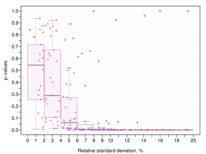
Figure S2: Results of consistency tests applied to simulated $1/f$ noise for the baseline (triangles) and the “slow drift” (diamonds) excess noise models. Horizontal axis: the relative standard deviation of the simulated timetrace $P_{\pm}(\mathrm{t})$. Triangles: combined $p$-values returned by the baseline model. Also depicted the box-and-whisker plots of groups of these values, with filled triangles representing outliers in each group. The diamonds depict the combined $p$-values returned by the “slow drift” test.

The results are plotted in Figure S2. Each symbol represents a simulation; its abscissa equals the RSD of the respective timetrace and its ordinate is the combined $p$-value obtained via consistency testing of the respective maximum likelihood estimate.

First we consider the baseline model results shown by triangles in Figure S2. For very low noise (essentially constant $P_{\pm}(\mathrm{t})$) the null hypothesis is expected to be true, and the $p$-values should be scattered approximately uniformly between $0$ and $1$, while for stronger noise we expect small $p$ to become progressively more likely.

To illustrate this transition more clearly, we have added to Figure S2 box-and-whisker plots of the same dataset, by binning the baseline $p$-values by the corresponding RSD, i.e., first group with RSD $<2\%$, second with $2\%\leq\text{RSD}<4\%$ and so on, up to $18\%\leq\text{RSD}<20\%$. The box-and-whisker plots are computed using the standard way, i.e., if $Q_{1}$, $Q_{2}$, $Q_{3}$ are the quartiles of the group and $\operatorname{IQR}=Q_{3}-Q_{1}$ is the interquartile range, then the lower and upper limits of the box are placed at $Q_{1}$ and $Q_{3}$, respectively, and the horizontal line within the box represents the median $Q_{2}$. Furthermore, the lower and upper fences are computed as $Q_{1}-1.5\operatorname{IQR}$ and $Q_{3}+1.5\operatorname{IQR}$, respectively; if any value in the group is below the lower or above the upper fence, it is considered an outlier and plotted with a filled symbol. Finally, whiskers are drawn so that the upper whisker is located either at the upper fence or the maximal value in the group (whichever is smaller); similarly, the lower whisker is located either at the lower fence or the minimal value in the group (whichever is larger).

As it can be observed in the Figure, the first two groups with RSD up to $4\%$ appear to be consistent with the standard uniform distribution. However, for relative standard deviation above 4% the distribution of the resulting $p$-values quickly deteriorates and for $\text{RSD}\geq 6\%$ already the median of the obtained $p$-values is well below the conventional $p=0.05$ threshold. We see a clear evidence of a threshold in environmental noise strengths (quantified by RSD in the simulation timetrace): if the noise is too low, the data are consistent with the baseline model. For larger values of RSD, the $p$-values for the baseline model collapse to very low values, indicating strong rejection of the null hypothesis of no excess noise.

Next we evaluate to what extent the data collected from $1/f$ noise simulations are consistent with single-timescale models discussed in the main text and in Supplementary Note IV.1 and IV.2. We have found that for this particular type of noise the behavior of the “fast fluctuator”’ test offers only a marginal improvement over the baseline model, hence the corresponding $p$-values are not plotted.

To the contrary, the “slow drift” model is generally consistent with the simulated data even if the excess noise level is high, provided that parameters of the Dirichlet distribution in the “slow drift model” (see Eq. 14) are chosen appropriately.

In Figure S2 the diamonds show the combined $p$-values for simulated noise data tested against the “slow drift” model using the Monte Carlo estimation procedure of Supplementary Note IV.2. Here we have used $\max\limits_{s=+,-}\sigma_{s}$ computed from the simulated timetrace $P_{\pm}(\mathrm{t})$ to set a priori the concentration parameter $\alpha_{\bullet}$ of the Dirichlet distribution used in the “slow drift” test. Despite the value of $\alpha_{\bullet}$ not being optimized (and hence, potentially biasing the test), the results indicate that the “slow drift” model for the data is not rejected: the $p$-values are high for the whole range of noise levels considered.

Example of statistical methodology applied to the simulated data

Here we illustrate in more detail application of statistical tests to a particular simulated timetrace of $1/f$ noise model. The simulation has used $\alpha_{\text{noise}}=10^{5.2}$ and $\left\langle P_{+}\right\rangle=$2.12\text{\times}{10}^{-05}$$, $\left\langle P_{-}\right\rangle=$6.9\text{\times}{10}^{-05}$$.

The estimated mean $\mu_{s}$ and the standard deviation $\sigma_{s}$ of the simulated $P_{\pm}(\mathrm{t})$ values are $\mu_{+}=$2.108\,606\,980\,390\,36\text{\times}{10}^{-05}$,\mu_{-}=$6.938\,102\,490\,875\,84\text{\times}{10}^{-05}$$ and $\sigma_{+}=$7.716\,197\,207\,933\,75\text{\times}{10}^{-07}$,\sigma_{-}=$1.368\,383\,497\,242\,68\text{\times}{10}^{-06}$$, which gives the relative standard deviation $\text{RSD}=$3.659\,381\,421$\%$. The simulated $P_{\pm}(\mathrm{t})$ values are well approximated by the normal distribution with the respective parameters; see the histograms of $P_{\pm}(\mathrm{t})$ in Figure S3b.

Next we describe how the spectrum of the simulated noise was analyzed. Let $R=2^{18}$, $K=\left\lfloor\frac{N_{\text{tot}}}{R}\right\rfloor=145$. Given the signal $P_{s}(n\,\tau_{0})$, $n=1,2,\ldots,N_{\text{tot}}$, where $s\in\{-,+\}$, its power spectral density (PSD) is estimated by splitting the signal into $K$ non-overlapping segments of length $R$ (the signal components with $n>KR$ are discarded) and computing the periodogram for each segment and averaging the results for the $K$ segments. Each periodogram is found by computing the squared magnitude of the discrete Fourier transform and dividing the result by $R$; moreover, the values at all frequencies except 0 and 0.5 are doubled since the one-sided periodogram is considered.

In Figure S3a we show the PSD estimates of the simulated timetrace which show the signature $1/f$ roll-off.

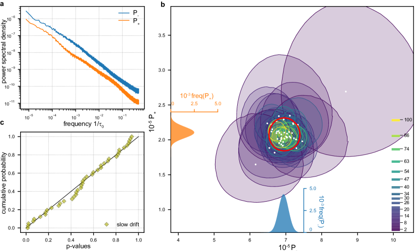
Figure S3: (a) The PSD estimates of the simulated timetrace. (b) White dots: maximum-likelihood estimates of $P_{\pm}$ in the baseline model for each sequence length separately. Also $p>0.05$ consistency regions are shown (color indicating the sequence length). The histograms of the simulated $P_{\pm}(\mathrm{t})$ values are depicted on the axes of the plot. (c) Empirical cumulative distribution of $p$-values for the slow drift model in comparison to the uniform distribution (black line).

Next, we analyze the simulated sample in the same way as the experimental data for device A, c.f. Figure 2 in the main text.

For the baseline model, the maximum likelihood gives the estimate $\left(P_{+},P_{-}\right)=\left($2.071\,61\text{\times}{10}^{-05}6.955\,32\text{\times}{10}^{-05}$\right)$, which correlates well with the underlying $\mu_{\pm}\pm\sigma_{\pm}$. Next, we employ Fisherian significance tests separately for each block of $N_{i}$ counts for a fixed burst length $t_{i}$ to define consistency regions of $p$-value greater than $0.05$ in the parameter space $(P_{+},P_{-})$ where the baseline model cannot be rejected at this significance level. These quasielliptic consistency regions are depicted in Figure S3b; again, their overlap is only partial. Fisher’s meta-analysis method yields the combined $p$-value $0.039\,145\,80$, thus the baseline model is nominally rejected.

The simulated data then were tested against the “slow drift” model with the optimized (as explained in Supplementary Note IV.2) parameters $\boldsymbol{\alpha}^{*}=($5.007\,829\,97\text{\times}{10}^{03}7.199\,349\,95\text{\times}{10}^{07}1.491\,559\,99\text{\times}{10}^{03}$)$. The cumulative distribution of the obtained $p$-values for each sequence length is shown in Figure S3c; it minimizes the empirical distance measure (15) and is close to being uniform. Quantitatively, the combined $p$-value equals $0.447\,131\,3$, implying that the simulated data are not inconsistent with the slow drift model.

The standard deviations of $P_{\pm}$ in the Dirichlet distribution $\operatorname{Dir}(\boldsymbol{\alpha}^{*})$ are $5.363\,933\text{\times}{10}^{-07}$ and $9.828\,273\text{\times}{10}^{-07}$, respectively, producing the $1\sigma$ estimates

$${P}_{+}=(2.07\pm 0.05)\times 10^{-5},\quad{P}_{-}=(6.96\pm 0.10)\times 10^{-5}\quad(\text{``slow drift'' estimate})$$

which compare well with $\mu_{\pm}\pm\sigma_{\pm}$ accessible for the simulated noise,

$$P_{+}=(2.11\pm 0.08)\times 10^{-5},\quad P_{-}=(6.94\pm 0.14)\times 10^{-5}\quad(\text{simulated noise})$$

Simulations of a single fluctuator

We have explored the excess noise model with a single fluctuator ($M=1$) with the switching rate $\Gamma_{1}$ varied in simulations from $10^{-6}\tau_{0}^{-1}$ to $\tau_{0}^{-1}$. The distribution of $P_{\pm}(\mathrm{t})$ in this case is bimodal, with the two modes, $P_{\pm}^{(1)}[0]$ and $P_{\pm}^{(1)}[1]$, chosen randomly before the start of the simulation. The corresponding noise power spectral density is a Lorentzian that crosses over from a constant to $1/f^{2}$ at frequency $f\sim\Gamma_{1}$.

With respect to the baseline and the “slow drift” statistical tests, the single-fluctuator model behaves similarly to the $1/f$ case considered above, regardless of the choice of $\Gamma_{1}$: a sufficiently large distance between the two modes generates counts inconsistent with the baseline, but compatible with the “slow drift” model with an appropriately chosen $\Delta P_{\pm}$.

The results of “fast flcutuator” tests do, in general, depend on the switching speed $\Gamma_{1}$: for fast $\Gamma_{1}\sim\tau_{0}^{-1}$ the simulated data typically are consistent with the “fast fluctuator” model, while for slower $\Gamma_{1}\ll\tau_{0}^{-1}$ the simulated data reject the “fast fluctuator” noise model.

These observations can be understood considering the characteristic frequencies to which our statistical tests are sensitive: “slow drift” probes the low-frequency part of the noise spectrum (switching rates on the order of $1/(N_{i}\tau_{0})\sim 10^{-5}\tau_{0}^{-1}$) while the “fast fluctuator” tests relatively high frequencies ($\sim\tau_{0}^{-1}$), at which the noise from a slow ($\Gamma_{1}\ll\tau^{-1}$) single fluctuator is sufficiently suppressed by the $1/f^{2}$ roll-off.

VI Slow drift model: variance of random walker’s position

In this section we derive the formula for the variance of the random walker’s position $\Delta x^{2}$ used in the concluding part of the main text.

Consider repeatedly sampling random walker’s position in the slow drift model; we are interested in the sample variance. However, the samples are correlated, since the model assumes using the same parameter $\boldsymbol{\theta}\sim\operatorname{Dir}(\boldsymbol{\alpha})$ for several ($N$) successive random walks. Henceforth, we consider the following scenario: draw $\boldsymbol{\theta}^{(1)}\sim\operatorname{Dir}(\boldsymbol{\alpha})$ and run $t$ steps of the random walk with step probabilities $\boldsymbol{\theta}^{(1)}$ for $N$ times; let $X_{1}^{(1)}$, $X_{2}^{(1)}$, $\ldots$, $X_{N}^{(1)}$ be the random walker’s position after the respective random walk has been completed. Afterwards, the step probabilities reset, i.e., a new parameter $\boldsymbol{\theta}^{(2)}\sim\operatorname{Dir}(\boldsymbol{\alpha})$ is independently drawn, and $N$ times random walk of $t$ steps is run with step probabilities $\boldsymbol{\theta}$, resulting in random variables $X_{1}^{(2)}$, $X_{2}^{(2)}$, $\ldots$, $X_{N}^{(2)}$. The process is continued until, say, $K$ blocks ${\mathbf{X}^{(k)}}:=\left(X^{(k)}_{1},X^{(k)}_{2},\ldots,X^{(k)}_{N}\right)$, $k=1,2,\ldots,K$, are obtained. It is important to stress that

1. the blocks ${\mathbf{X}^{(1)}},{\mathbf{X}^{(2)}},\ldots,{\mathbf{X}^{(K)}}$ are assumed to be pairwise independent;

2. within each block, variables $X_{i}^{(k)}$ and $X_{j}^{(k)}$, $i\neq j$, $k=1,2,\ldots,K$, are assumed to be conditionally independent given $\boldsymbol{\theta}^{(k)}$, i.e.,

   $$(X_{i}^{(k)}\perp\!\!\!\perp X_{j}^{(k)})\mid\boldsymbol{\theta}^{(k)}.$$

Let $M:=KN$; we are interested in the quantity

$$S:=\frac{1}{M}\sum_{k=1}^{K}\sum_{i=1}^{N}\left(X^{(k)}_{i}-\overline{X}\right)^{2},$$

where $\overline{X}:=\frac{1}{M}\sum_{k=1}^{K}\sum_{i=1}^{N}X_{i}^{(k)}$. In particular, the task is to find $\Delta x^{2}:=\operatorname{E}(S)$ in the $K\to\infty$ limit.

Claim 3.

The expectation $\Delta x^{2}=\operatorname{E}(S)$ in the $P_{\pm}\ll 1$, $K\to\infty$ limit satisfies

$$\Delta x^{2}=\frac{A}{1+\alpha_{\bullet}}\left(\frac{t\alpha_{\bullet}(M-1)}{M}+\frac{t^{2}(K-1)}{K}\right)\approx(\langle P_{+}\rangle+\langle P_{\pm}\rangle)\,t+(\Delta P_{+}^{2}+\Delta P_{-}^{2})\,t^{2},$$

where

$$A:=\left(\tilde{\alpha}_{-1}+\tilde{\alpha}_{1}\right)-\left(\tilde{\alpha}_{-1}-\tilde{\alpha}_{1}\right)^{2};$$

$$\tilde{\alpha}_{\pm 1}:=\frac{\alpha_{\pm 1}}{\alpha_{\bullet}};\quad\alpha_{\bullet}:=\alpha_{-1}+\alpha_{0}+\alpha_{1};$$

$$\langle P_{\pm}\rangle:=\operatorname{E}(P_{\pm})=\tilde{\alpha}_{\pm 1};$$

$$\Delta P_{\pm}^{2}:=\operatorname{Var}(P_{\pm})=\frac{\tilde{\alpha}_{\pm 1}(1-\tilde{\alpha}_{\pm 1})}{1+\alpha_{\bullet}}.$$

Proof.

We start by noting that each block $\mathbf{X}^{(k)}$ is an independent observation of the random variable $\mathbf{X}=(X_{1},X_{2},\ldots,X_{N})$, where $\mathbf{X}$ is obtained by the process above with $K=1$. Let us define a random variable $Y=\frac{1}{N}(X_{1}+\ldots+X_{N})$, then there are $K$ iid variables $Y_{1},\ldots,Y_{K}\sim Y$ corresponding to the blocks $\mathbf{X}^{(1)}$, …, $\mathbf{X}^{(K)}$ . We can express

$$S=\frac{1}{M}\sum_{i,k}\left(X^{(k)}_{i}\right)^{2}-\frac{2}{M}\sum_{i,k}\left(X^{(k)}_{i}\right)\overline{X}+\overline{X}^{2}=\frac{1}{M}\sum_{i,k}\left(X^{(k)}_{i}\right)^{2}-\overline{X}^{2}$$

and

$$\overline{X}=\frac{1}{K}(Y_{1}+Y_{2}+\ldots+Y_{K}).$$

Since $X^{(k)}_{i}$ are identically distributed, we have

$$\operatorname{E}\left(\frac{1}{M}\sum_{k=1}^{K}\sum_{i=1}^{N}\left(X^{(k)}_{i}\right)^{2}\right)=\frac{M}{M}\cdot\operatorname{E}(X_{1}^{2})=\operatorname{Var}(X_{1})+\operatorname{E}(X_{1})^{2};$$

since $Y_{1},\ldots,Y_{K}$ are iid, we have

$$(Y_{1}+Y_{2}+\ldots+Y_{K})^{2}=\sum_{k=1}^{K}Y_{k}^{2}+\sum_{k=1}^{K}\sum_{\begin{subarray}{c}l=1\\ l\neq k\end{subarray}}^{K}Y_{k}Y_{l}$$

and

$$\operatorname{E}\left(\overline{X}^{2}\right)=\frac{1}{K}\operatorname{E}(Y^{2})+\frac{K-1}{K}\operatorname{E}(Y)^{2}=\frac{1}{K}\operatorname{Var}(Y)+\operatorname{E}(Y)^{2}.$$

Consequently,

$$\Delta x^{2}=\operatorname{Var}(X_{1})+\operatorname{E}(X_{1})^{2}-\frac{1}{K}\operatorname{Var}(Y)-\operatorname{E}(Y)^{2}.$$

Let us show that

$$\operatorname{E}(X_{1})=t\left(\tilde{\alpha}_{1}-\tilde{\alpha}_{-1}\right)$$ (18)

$$\operatorname{Var}(X_{1})=\frac{At\alpha_{\bullet}}{1+\alpha_{\bullet}}+\frac{At^{2}}{1+\alpha_{\bullet}},$$ (19)

$$\operatorname{E}(Y)=\operatorname{E}(X_{1}),$$ (20)

$$\operatorname{Var}(Y)=\frac{At\alpha_{\bullet}}{N(1+\alpha_{\bullet})}+\frac{At^{2}}{1+\alpha_{\bullet}},$$ (21)

then we will arrive at

$$\Delta x^{2}=\operatorname{Var}(X_{1})-\frac{1}{K}\operatorname{Var}(Y)=\frac{At\alpha_{\bullet}(M-1)}{M(1+\alpha_{\bullet})}+\frac{At^{2}(K-1)}{K(1+\alpha_{\bullet})},$$

as desired.

Equalities (18) and (19). If $\boldsymbol{\theta}=(P_{-},P_{0},P_{+})$ is a fixed parameter, then the position of the random walker after $t$ steps with step probabilities given by $\boldsymbol{\theta}$ is given by $\delta_{1}+\ldots+\delta_{t}$, where $\delta_{i}\sim\delta$ are iid and

$$\delta=\begin{cases}\ -1,&\text{ with prob. }P_{-},\\ 0,&\text{ with prob. }P_{0},\\ +1,&\text{ with prob. }P_{+}.\end{cases}$$

Consequently, for the Dirichlet-distributed $\boldsymbol{\theta}$ the conditional expectation / variance $\operatorname{E}(X_{1}\mid\boldsymbol{\theta})$ and $\operatorname{Var}(X_{1}\mid\boldsymbol{\theta})$ satisfy

$$\operatorname{E}(X_{1}\mid\boldsymbol{\theta})=t\left(P_{+}-P_{-}\right)$$

$$\operatorname{Var}(X_{1}\mid\boldsymbol{\theta})=t\left(P_{+}+P_{-}\right)-t\left(P_{+}-P_{-}\right)^{2}.$$

By the laws of total expectation / variance, we obtain (18) and (19):

$$\operatorname{E}(X_{1}) =\operatorname{E}\left(\operatorname{E}(X_{1}\mid\boldsymbol{\theta})\right)=t(\tilde{\alpha}_{1}-\tilde{\alpha}_{-1})$$

$$\operatorname{Var}(X_{1}) =\operatorname{E}(\operatorname{Var}(X_{1}\mid\boldsymbol{\theta}))+\operatorname{Var}(\operatorname{E}(X_{1}\mid\boldsymbol{\theta}))$$

$$=t\operatorname{E}\left(P_{+}+P_{-}+2P_{+}P_{-}-P_{+}^{2}-P_{-}^{2}\right)+t^{2}\operatorname{Var}\left(P_{+}-P_{-}\right)$$

$$=\frac{t\alpha_{\bullet}A}{1+\alpha_{\bullet}}+\frac{t^{2}A}{1+\alpha_{\bullet}}.$$

To show the last equality, recall the relevant properties of $(P_{-},P_{0},P_{+})\sim\operatorname{Dir}(\boldsymbol{\alpha})$:

$$\operatorname{E}(P_{\pm})={\tilde{\alpha}}_{\pm 1};$$

$$\operatorname{Var}(P_{\pm})=\frac{\tilde{\alpha}_{\pm 1}(1-\tilde{\alpha}_{\pm 1})}{1+\alpha_{\bullet}};$$

$$\operatorname{Cov}(P_{+};P_{-})=\frac{-\tilde{\alpha}_{-1}\tilde{\alpha}_{1}}{1+\alpha_{\bullet}}.$$

Thus

$$\operatorname{Var}\left(P_{+}-P_{-}\right)=\operatorname{Var}\left(P_{+}\right)+\operatorname{Var}\left(P_{-}\right)-2\operatorname{Cov}(P_{+};P_{-})=\frac{A}{1+\alpha_{\bullet}}$$

and

$$\operatorname{E}\left(P_{+}+P_{-}+2P_{+}P_{-}-P_{+}^{2}-P_{-}^{2}\right)$$

$$=\operatorname{E}\left(P_{+}+P_{-}\right)+2\left(\operatorname{Cov}(P_{+};P_{-})+\operatorname{E}(P_{+})\operatorname{E}(P_{-})\right)-\left(\operatorname{Var}\left(P_{+}\right)+\operatorname{E}(P_{+})^{2}\right)-\left(\operatorname{Var}\left(P_{-}\right)+\operatorname{E}(P_{-})^{2}\right)$$

$$=\operatorname{E}\left(P_{+}+P_{-}\right)-\left(\operatorname{E}\left(P_{+}-P_{-}\right)\right)^{2}-\operatorname{Var}\left(P_{+}-P_{-}\right)$$

$$=A-\frac{A}{1+\alpha_{\bullet}}=\frac{\alpha_{\bullet}A}{1+\alpha_{\bullet}}.$$

Equality (20). This equality trivially follows from the definition of $Y$ and the fact that $X_{i}$ are identically distributed:

$$\operatorname{E}(Y)=\frac{1}{N}\operatorname{E}(X_{1}+\ldots+X_{N})=\frac{N}{N}\operatorname{E}(X_{1}).$$

Equality (21). The variance of the sum $X_{1}+\ldots+X_{N}$ is the sum of the covariances:

$$\operatorname{Var}(X_{1}+\ldots+X_{N})=\sum_{i=1}^{N}\operatorname{Var}(X_{i})+2\sum_{1\leq i<j<N}\operatorname{Cov}(X_{i},X_{j})$$

However, $X_{i}$ are identically distributed, therefore

$$\operatorname{Var}(Y)=\frac{1}{N^{2}}\left(N\operatorname{Var}(X_{1})+(N^{2}-N)\operatorname{Cov}(X_{1},X_{2})\right)$$ (22)

$\operatorname{Var}(X_{1})$ is given by (19), it remains to find $\operatorname{Cov}(X_{1},X_{2})$. By the law of total covariance,

$$\operatorname{Cov}(X_{1},X_{2})=\operatorname{E}\left(\operatorname{Cov}\left(X_{1},X_{2}\mid\boldsymbol{\theta}\right)\right)+\operatorname{Cov}\left(\operatorname{E}\left(X_{1}\mid\boldsymbol{\theta}\right),\operatorname{E}\left(X_{2}\mid\boldsymbol{\theta}\right)\right)$$

Since $X_{1},X_{2}$ are conditionally independent given $\boldsymbol{\theta}$, the conditional covariance vanishes: $\operatorname{Cov}\left(X_{1},X_{2}\mid\boldsymbol{\theta}\right)=0$. Moreover, as $X_{1},X_{2}$ are identically distributed,

$$\operatorname{E}\left(X_{1}\mid\boldsymbol{\theta}\right)=\operatorname{E}\left(X_{2}\mid\boldsymbol{\theta}\right)=t\left(P_{+}-P_{-}\right),$$

thus

$$\operatorname{Cov}(X_{1},X_{2})=t^{2}\operatorname{Var}\left(P_{+}-P_{-}\right)=\frac{t^{2}A}{1+\alpha_{\bullet}}.$$

We arrive at

$$\operatorname{Var}(Y)=\frac{1}{N}\left(A\cdot\frac{t\alpha_{\bullet}+t^{2}}{1+\alpha_{\bullet}}+(N-1)\frac{t^{2}A}{1+\alpha_{\bullet}}\right)=\frac{At\alpha_{\bullet}}{N(1+\alpha_{\bullet})}+\frac{At^{2}}{1+\alpha_{\bullet}},$$

which concludes the proof. ∎

VII Proof for spread condition

This section contains the proof for the spread condition shown in (2) in the main text (restated here for convenience).

Claim 4.

For any random process on the line with steps of length 1, the spread condition

$$\sum\limits_{y=-\infty}^{x-1}p_{y}^{t}\leq\sum\limits_{y=-\infty}^{x}p_{y}^{t+1}\leq\sum\limits_{y=-\infty}^{x+1}p_{y}^{t}\quad\text{for all }x,$$ (23)

must be satisfied.

Proof.

If the random process is at location $y\leq x-1$ after $t$ time steps, it must be at a location $y^{\prime}\leq x$ after $t+1$ time steps. Hence, $\sum_{y=-\infty}^{x-1}p_{y}^{t}\leq\sum_{y=-\infty}^{x}p_{y}^{t+1}$.

On the other hand, if the process is at a location $y\leq x$ after $t+1$ time steps, it has been at a location $y^{\prime}\leq x+1$ after $t$ time steps. Hence, $\sum_{y=-\infty}^{x}p_{y}^{t+1}\leq\sum_{y=-\infty}^{x+1}p_{y}^{t}$. ∎

We note that the claim applies not just to Markov processes but to any random process that can move at most distance 1 in one time step. For example, it applies to processes where the transition probabilities depend not just on the current location but also on locations in previous time steps.

Claim 5.

If two probability distributions $(p_{x}^{t})_{x\in\mathbb{Z}}$ and $(p_{x}^{t+1})_{x\in\mathbb{Z}}$ satisfy the spread condition (23), then there exists a set of transition probabilities $P_{\pm 1}^{(x,t)}$ such that $(p_{x}^{t+1})_{x\in\mathbb{Z}}$ is generated from $(p_{x}^{t})_{x\in\mathbb{Z}}$ by a Markov process

$$p_{x}^{t+1}=P_{+1}^{(x-1,t)}p_{x-1}^{t}+\left(1-P_{+1}^{(x,t)}-P_{-1}^{(x,t)}\right)p_{x}^{t}+P_{-1}^{(x+1,t)}p_{x+1}^{t},\quad x\in\mathbb{Z}.$$

Proof.

Let $q_{x}^{t}=\sum_{y=-\infty}^{x}p_{y}^{t}$; then the spread condition is equivalent to

$$q^{t}_{x-1}\leq q^{t+1}_{x}\leq q^{t}_{x+1},\quad\text{for all }x\in\mathbb{Z}.$$

Consider a Markov process in which the probability of moving left from a location $x$ at time $t$ is defined by

$$P_{-1}^{(x,t)}=\begin{cases}0&\text{if }q_{x-1}^{t}\geq q_{x-1}^{t+1}\\ \frac{1}{p_{x}^{t}}\left({q_{x-1}^{t+1}-q_{x-1}^{t}}\right)&\text{otherwise},\end{cases}$$

and the probability of moving right is defined by

$$P_{+1}^{(x,t)}=\begin{cases}0&\text{if }q_{x}^{t}\leq q_{x}^{t+1}\\ \frac{1}{p_{x}^{t}}\left({q_{x}^{t}-q_{x}^{t+1}}\right)&\text{otherwise}.\end{cases}$$

The probability to stay at $x$ is defined as $P_{0}^{(x,t)}:=1-P_{+1}^{(x,t)}-P_{-1}^{(x,t)}$. Notice that the spread condition implies

$$q_{x-1}^{t+1}-q_{x-1}^{t}\leq q_{x}^{t}-q_{x-1}^{t}=p_{x}^{t}\quad\text{and}\quad q_{x}^{t}-q_{x}^{t+1}=q_{x-1}^{t}+p^{t}_{x}-q_{x}^{t+1}\leq p^{t}_{x},$$

thus $P_{-1}^{(x,t)}\leq 1$ and $P_{+1}^{(x,t)}\leq 1$. Finally, we have $P_{0}^{(x,t)}\geq 0$. To see that, it suffices to consider the case when $P_{+1}^{(x,t)}$ and $P_{-1}^{(x,t)}$ are both positive; then we have to show

$$\left({q_{x}^{t}-q_{x}^{t+1}}\right)+\left({q_{x-1}^{t+1}-q_{x-1}^{t}}\right)\leq p^{t}_{x}.$$

However, this inequality clearly holds, since

$$\left({q_{x}^{t}-q_{x}^{t+1}}\right)+\left({q_{x-1}^{t+1}-q_{x-1}^{t}}\right)=\left({q_{x}^{t}-q_{x-1}^{t}}\right)+\left({q_{x-1}^{t+1}-q_{x}^{t+1}}\right)=p^{t}_{x}-p^{t+1}_{x}\leq p^{t}_{x}.$$

Therefore we have defined valid transition probabilities.

To see that this process produces $(p_{x}^{t+1})_{x\in\mathbb{Z}}$, let $\overline{q}_{x}^{t+1}$ be the probability of being at a location $x^{\prime}\leq x$ after applying these transition probabilities to the distribution $(p_{x}^{t})_{x\in\mathbb{Z}}$. We show that $\overline{q}_{x}^{t+1}=q_{x}^{t+1}$ for all $x$, thus the probability of being at any particular $x_{0}$ equals $q_{x_{0}}^{t+1}-q_{x_{0}-1}^{t+1}=p_{x_{0}}^{t+1}$. We consider two cases.

1. If $q_{x}^{t}\leq q_{x}^{t+1}$, we have $P_{+1}^{(x,t)}=0$ and

   $$\overline{q}_{x}^{t+1}=q_{x}^{t}+p_{x+1}^{t}P_{-1}^{(x+1,t)}=q_{x}^{t}+\left(q_{x}^{t+1}-q_{x}^{t}\right)=q^{t+1}_{x}.$$

2. If $q_{x}^{t}>q_{x}^{t+1}$, we have $P_{-1}^{(x+1,t)}=0$ and

   $$\overline{q}_{x}^{t+1}=q_{x-1}^{t}+p_{x}^{t}\left(1-P_{+1}^{(x,t)}\right)=q_{x-1}^{t}+p_{x}^{t}-\left(q_{x}^{t}-q_{x}^{t+1}\right)=q_{x}^{t+1},$$

which concludes the proof. ∎

A consequence of these two claims is that, given just the probabilities $p_{x}^{t}$, we cannot distinguish whether they come from a (possibly non-stationary, not translation-invariant) Markov process or from a more general process that moves at most distance 1 in one time step. (In the second case, the spread condition will be satisfied and then, because of Claim 5, there will be a time and location dependent Markov process that gives the same $p_{x}^{t}$.)

References

- (1) Bäuerle, C. et al. Coherent control of single electrons: a review of current progress. Rep. Prog. Phys. 81, 056503 (2018).
- (2) Pekola, J. P. et al. Single-electron current sources: Toward a refined definition of the ampere. Rev. Mod. Phys. 85, 1421–1472 (2013).
- (3) DiVincenzo, D. P. The Physical Implementation of Quantum Computation. Fortschr. Phys. 48, 771–783 (2000).
- (4) Chow, J. M. et al. Universal Quantum Gate Set Approaching Fault-Tolerant Thresholds with Superconducting Qubits. Phys. Rev. Lett. 109, 060501 (2012).
- (5) Barends, R. et al. Superconducting quantum circuits at the surface code threshold for fault tolerance. Nature 508, 500–503 (2014).
- (6) Benhelm, J., Kirchmair, G., Roos, C. F. & Blatt, R. Towards fault-tolerant quantum computing with trapped ions. Nat. Phys. 4, 463–466 (2008).
- (7) Gaebler, J. et al. High-Fidelity Universal Gate Set for Ion Qubits. Phys. Rev. Lett. 117, 060505 (2016).
- (8) Ballance, C. J., Harty, T. P., Linke, N. M., Sepiol, M. A. & Lucas, D. M. High-Fidelity Quantum Logic Gates Using Trapped-Ion Hyperfine Qubits. Phys. Rev. Lett. 117, 060504 (2016).
- (9) Emerson, J., Alicki, R. & Życzkowski, K. Scalable noise estimation with random unitary operators. J. Opt. B: Quantum Semiclassical Opt. 7, S347–S352 (2005).
- (10) Knill, E. et al. Randomized benchmarking of quantum gates. Phys. Rev. A 77 (2008).
- (11) Magesan, E., Gambetta, J. M. & Emerson, J. Scalable and Robust Randomized Benchmarking of Quantum Processes. Phys. Rev. Lett. 106, 180504 (2011).
- (12) Huang, W. et al. Fidelity benchmarks for two-qubit gates in silicon. Nature 569, 532–536 (2019).
- (13) Erhard, A. et al. Characterizing large-scale quantum computers via cycle benchmarking. Nat. Commun. 10, 1–7 (2019).
- (14) Arute, F. et al. Quantum supremacy using a programmable superconducting processor. Nature 574, 505–510 (2019).
- (15) Aharonov, D. & Ben-Or, M. Fault-tolerant quantum computation with constant error rate. SIAM J. Comput. (2008).
- (16) Fowler, A. G., Mariantoni, M., Martinis, J. M. & Cleland, A. N. Surface codes: Towards practical large-scale quantum computation. Phys. Rev. A 86, 032324 (2012).
- (17) Stein, F. et al. Validation of a quantized-current source with 0.2 ppm uncertainty. Appl. Phys. Lett. 107, 103501 (2015).
- (18) Takada, S. et al. Sound-driven single-electron transfer in a circuit of coupled quantum rails. Nat. Commun. 10, 1–9 (2019).
- (19) Mills, A. R. et al. Shuttling a single charge across a one-dimensional array of silicon quantum dots. Nat. Commun. 10, 1063 (2019).
- (20) Nakajima, T. et al. Quantum non-demolition measurement of an electron spin qubit. Nat. Nanotechnol. 14, 555–560 (2019).
- (21) Freise, L. et al. Trapping and Counting Ballistic Nonequilibrium Electrons. Physical Review Letters 124, 127701 (2020).
- (22) Smirne, A., Kołodyński, J., Huelga, S. F. & Demkowicz-Dobrzański, R. Ultimate precision limits for noisy frequency estimation. Phys. Rev. Lett. 116, 120801 (2016).
- (23) Giovannetti, V., Lloyd, S. & Maccone, L. Advances in quantum metrology. Nature Photonics 5, 222–229 (2011).
- (24) Ball, H., Stace, T. M., Flammia, S. T. & Biercuk, M. J. Effect of noise correlations on randomized benchmarking. Phys. Rev. A 93, 022303 (2016).
- (25) Epstein, J. M., Cross, A. W., Magesan, E. & Gambetta, J. M. Investigating the limits of randomized benchmarking protocols. Physical Review A 89, 062321 (2014).
- (26) O’Malley, P. J. J. et al. Qubit Metrology of Ultralow Phase Noise Using Randomized Benchmarking. Phys. Rev. Appl 3, 044009 (2015).
- (27) Kaestner, B. & Kashcheyevs, V. Non-adiabatic quantized charge pumping with tunable-barrier quantum dots: a review of current progress. Rep. Prog. Phys. 78, 103901 (2015).
- (28) Kaestner, B. et al. Single-parameter nonadiabatic quantized charge pumping. Phys. Rev. B 77, 153301 (2008).
- (29) Kashcheyevs, V. & Kaestner, B. Universal Decay Cascade Model for Dynamic Quantum Dot Initialization. Phys. Rev. Lett. 104, 186805 (2010).
- (30) Gerster, T. et al. Robust formation of quantum dots in GaAs/AlGaAs heterostructures for single-electron metrology. Metrologia 56, 014002 (2018).
- (31) Giblin, S. P. et al. Evidence for universality of tunable-barrier electron pumps. Metrologia 56, 044004 (2019).
- (32) Fricke, L. et al. Quantized current source with mesoscopic feedback. Phys. Rev. B 83, 193306 (2011).
- (33) Mavadia, S. et al. Experimental quantum verification in the presence of temporally correlated noise. npj Quantum Inf. 4, 1–9 (2018).
- (34) Christensen, R. Testing Fisher Neyman Pearson and Bayes. Am. Stat. 59, 121–126 (2005).
- (35) Borenstein, M., Hedges, L. V., Higgins, J. P. T. & Rothstein, H. R. Meta-Analysis Methods Based on Direction and p-Values, chap. 36, 325–330 (John Wiley & Sons, Chichester, 2009).
- (36) Fisher, R. A. Statistical methods for research workers (Oliver & Boyd, Edinburgh, 1932), fourth ed. - revised and enlarged edn.
- (37) Paladino, E., Galperin, Y. M., Falci, G. & Altshuler, B. L. noise: Implications for solid-state quantum information. Rev. Mod. Phys. 86, 361–418 (2014).
- (38) Ng, K. W., Tian, G.-L. & Tang, M.-L. Dirichlet and related distributions: Theory methods and applications. (John Wiley & Sons, Hoboken, 2011).
- (39) Johnson, N. L., Kotz, S. & Balakrishnan, N. Discrete multivariate distributions. Wiley series in probability and statistics (Wiley, New York, 1997).
- (40) Jenei, M. et al. Waiting time distributions in a two-level fluctuator coupled to a superconducting charge detector. Physical Review Research 1, 033163 (2019).
- (41) Ridley, B. K. Hot electrons in low-dimensional structures. Rep. Prog. Phys. 54, 169–256 (1991).
- (42) Snoke, D. W., Rühle, W. W., Lu, Y.-C. & Bauser, E. Evolution of a nonthermal electron energy distribution in GaAs. Phys. Rev. B 45, 10979–10989 (1992).
- (43) Molenkamp, L. W., Brugmans, M. J. P., van Houten, H. & Foxon, C. T. Electron-electron scattering probed by a collimated electron beam. Semicond. Sci. Technol. 7, B228 (1992).
- (44) Yamahata, G., Giblin, S. P., Kataoka, M., Karasawa, T. & Fujiwara, A. Gigahertz single-electron pumping in silicon with an accuracy better than 9.2 parts in 107. Applied Physics Letters 109, 013101 (2016).
- (45) Fricke, L. et al. Self-Referenced Single-Electron Quantized Current Source. Phys. Rev. Lett. 112, 226803 (2014).
- (46) Schoelkopf, R. J., Wahlgren, P., Kozhevnikov, A. A., Delsing, P. & Prober, D. E. The radio-frequency single-electron transistor RF-SET: A fast and ultrasensitive electrometer. Science 280, 1238–1242 (1998).
- (47) Zhang, X.-K., Wan, J., Lu, J.-J. & Xu, X.-P. Recurrence and Pólya Number of General One-Dimensional Random Walks. Commun. Theor. Phys. 56, 293–296 (2011).
- (48) Shimizu, K. & Yanagimoto, T. The inverse trinomial distribution. Jpn. J. Appl. Phys. 20, 89–96 (1991). In Japanese.
- (49) Aoyama, K. & Shimizu, K. A generalization of the inverse trinomial. Tech. Rep., Keio University. Department of Mathematics (2005). KSTS/RR-05/003.
- (50) NIST Digital Library of Mathematical Functions, Release 1.0.27 of 2020-06-15. URL http://dlmf.nist.gov/. F. W. J. Olver, A. B. Olde Daalhuis, D. W. Lozier, B. I. Schneider, R. F. Boisvert, C. W. Clark, B. R. Miller, B. V. Saunders, H. S. Cohl, and M. A. McClain, eds.
- (51) Erdélyi, A., Magnus, W., Oberhettinger, F. & Tricomi, F. G. Higher Transcendental Functions. Vol. I (McGraw-Hill Book Company, Inc., New York-Toronto-London, 1953).
- (52) Eichstädt, S. & Wilkens, V. GUM2DFT—a software tool for uncertainty evaluation of transient signals in the frequency domain. Meas. Sci. Technol. 27, 055001 (2016).
- (53) Conover, W. J. A Kolmogorov Goodness-of-Fit Test for Discontinuous Distributions. J. Am. Stat. Assoc. 67, 591–596 (1972).
- (54) Smith, P. J., Rae, D. S., Manderscheid, R. W. & Silbergeld, S. Approximating the Moments and Distribution of the Likelihood Ratio Statistic for Multinomial Goodness of Fit. J. Am. Stat. Assoc. 76, 737–740 (1981).
- (55) Cressie, N. & Read, T. R. C. Multinomial Goodness-of-Fit Tests. J. R. Stat. Soc. Ser. B Methodol. 46, 440–464 (1984).
- (56) Jann, B. Multinomial goodness–of–fit: Large–sample tests with survey design correction and exact tests for small samples. SJ 08, 122584 (2008).
- (57) Barnard, G. A. Discussion of The spectral analysis of point processes by M. S. Bartlett. J. R. Stat. Soc. Ser. B Methodol. 25, 294 (1963).
- (58) Hope, A. C. A. A Simplified Monte Carlo Significance Test Procedure. J. R. Stat. Soc. Ser. B Methodol. 30, 582–598 (1968).
- (59) Besag, J. Simple Monte Carlo P-Values. In Page, C. & LePage, R. (eds.) Computing Science and Statistics, 158–162 (Springer New York, New York, NY, 1992).
- (60) Winkler, A. M. et al. Non-parametric combination and related permutation tests for neuroimaging. Hum. Brain Mapp. 37, 1486–1511 (2016).
- (61) Mielke Jr, P. W., Johnston, J. E. & Berry, K. J. Combining Probability Values from Independent Permutation Tests: A Discrete Analog of Fishers Classical Method. Psychol. Rep. 95, 449–458 (2004).