∎

¹¹institutetext: School of Computer Science, Engineering and Mathematics
Flinders University, Adelaide, Australia
Tel.: +61 8 82012841
¹¹email: {davoud.mougouei,david.powers}@flinders.edu.au

Modeling and Selection of Interdependent Software Requirements using Fuzzy Graphs

Davoud Mougouei David M. W. Powers

(This is a post-peer-review, pre-copyedit version of an article published in International Journal of Fuzzy Systems. The final authenticated version is available online at: http://dx.doi.org/10.1007/s40815-017-0364-4.)

Abstract

Software requirement selection is to find an optimal set of requirements that gives the highest value for a release of software while keeping the cost within the budget. However, value-related dependencies among software requirements may impact the value of an optimal set. Moreover, value-related dependencies can be of varying strengths. Hence, it is important to consider both the existence and the strengths of value-related dependencies during a requirement selection. The existing selection models however, either assume that software requirements are independent or they ignore strengths of requirement dependencies. This paper presents a cost-value optimization model that considers the impacts of value-related requirement dependencies on the value of selected requirements (optimal set). We have exploited algebraic structure of fuzzy graphs for modeling value-related requirement dependencies and their strengths. Validity and practicality of the work are verified through carrying out several simulations and studying a real world software project.

1 Introduction

Owing to budget constraints, it is hardly if ever feasible to fully implement the requirements of a software release bagnall_next_2001 . Therefore, requirement selection is needed to find an optimal set of requirements with the highest value while keeping the cost within the budget mougouei2019fuzzy ; mougouei2015partial ; dahlstedt_moulding_2003 ; barney_product_2008 ; ruhe_product_2010 ; achimugu_systematic_2014 ; kukreja_value_based_2013 ; Fogelstr_Usingportfolio_2010 . This problem, also known as the Next Release Problem (NRP) bagnall_next_2001 , is mathematically formulated as a Binary Knapsack Problem (BKP) mougouei2017integer ; harman_exact_2014 ; szoke_conceptual_2011 ; zhang_multi_objective_2007 ; carlshamre_release_2002 ; lust_multiobjective_2012 ; karlsson_optimizing_1997 ; jung_optimizing_1998 .

Based on the BKP formula, the existing selection models aim to maximize the Accumulated Value (AV) of an optimal set on the assumption that the value of an optimal is derived by accumulating the Estimated Values (EV s) of selected software requirement harman_exact_2014 . However, several studies have argued that this assumption does not hold when interdependencies exist among requirements carlshamre_release_2002 ; van_den_akker_flexible_2005 ; harman_exact_2014 ; mougouei2016factoring . The reason is that software requirements affect each other’s values due to the value-related dependencies among them mougouei2020dependency ; mougouei2019dependency ; mougouei2018mathematical ; mougouei2017dependency ; mougouei2017modeling ; dahlstedt_requirements_2005 ; carlshamre_release_2002 ; karlsson_improved_1997 . As a result, excluded requirements may impact the values of selected requirements that depend on them. Hence the actual value i.e. Customer Value (CV) of a selected requirement might differ from its estimated value (EV).

On the other hand, value-related requirement dependencies can be of various strengths in the context of real world projects dahlstedt_moulding_2003 ; Robinson_RIM_2003 ; ramesh_toward_2001 . In other words, values of requirements can weakly, moderately, or strongly depend on each other wang_simulation_2012 . Therefore, it is important to consider both the existence and the strengths of value-related requirement dependencies brasil_multiobjective_2012 ; harman_exact_2014 while considering the impacts of requirements on each other’s values during a requirement selection.

However, the existing requirement selection models either assume that requirements are independent karlsson_optimizing_1997 ; jung_optimizing_1998 ; zhang_multi_objective_2007 ; finkelstein2009search ; del2010ant or they formulate requirement dependencies as precedence constraints of BKP formula without considering the strengths of those dependencies bagnall_next_2001 ; li2016value ; veerapen2015integer ; greer_software_2004 ; ruhe_quantitative_2003 ; van2011quantitative ; zhang2010search ; saliu2007bi ; van2005determination ; ngo2009optimized ; chen2013ant ; xuan2012solving ; van2008software . In the latter case, dependencies are considered as binary (0/1) relations.

As such, by excluding a requirement from an optimal set, all of its dependent requirements also have to be excluded even if the budget allows for their implementation li_integrated_2010 . This problem is referred to as Selection Deficiency Problem (SDP) mougouei2016factoring . As a result of the SDP, any small increase in the number of dependencies would dramatically depreciate the accumulated value of an optimal set li_integrated_2010 . Hence, the SDP can severely impact the efficiency of selection models that formulate all requirement dependencies as precedence relations.

This paper has focused on considering the impacts of value-related requirement dependencies on the value of an optimal set during a selection process. We have achieved this through considering both the existence and the strengths of value-related requirement dependencies during software requirement selection. In doing so, we have specially made three main contributions.

First, we have demonstrated using algebraic structure of fuzzy graphs kalampakas_fuzzy_2013 ; zimmermann_fuzzy_1996 ; rosenfeld_fuzzygraph_1975 ; mordeson_fuzzy_2001 to modeling value-related requirement dependencies and their strengths.

Second, we have proposed a new measure of value of an optimal set referred to as Overall Value (OV) that considers the impacts of value-related requirement dependencies on the value of an optimal set (selected requirements). In this regard, we have introduced the following definitions of value.

•

Estimated Value (EV): Value of a software requirement estimated by the stakeholders.
•

Customer Value (CV): Value of a software requirement derived by considering the impacts of value-related dependencies on the estimated value of that requirement.
•

Accumulated Value (AV): a measure of value of an optimal set that is derived by accumulating the estimated values of selected requirements without considering value-related dependencies.
•

Overall Value (OV): a measure of value of an optimal set that is derived by accumulating the customer values of selected requirements with the consideration of the impacts of value-related requirement dependencies on the value of the selected requirements.

Finally, we have presented a novel requirement selection model referred to as the GORS (Graph Oriented Requirement Selection), which maximizes the overall value of an optimal set while mitigating the SDP. The proposed model not only considers value-related dependencies among requirements but more importantly explicitly factors in the strengths of those dependencies.

Validity and practicality of the work are verified through a) carrying out several simulations and b) studying a real world software project. The results of our simulations as well as a case study of a real world software project have consistently shown that: (a) the GORS model can properly capture the strengths of value-related dependencies among requirements during a selection process while mitigating the selection deficiency problem (SDP), (b) the GORS model always maximizes the overall value of an optimal set, and (c) maximizing the overall and the accumulated values of an optimal set can be conflicting objectives korte_combinatorial_2006 as maximizing one may depreciate the other.

The remainder of this paper is organized as follows. We first discuss related works in Section 2. Then, Section 3 gives the details of modeling value-related requirement dependencies by fuzzy graphs. After that, Section 4 introduces our proposed formulation of overall value of an optimal set as well as our proposed graph oriented requirement selection (GORS) model. The results of our simulations and a case study of a real world software project are discussed in Section 5. Section 6 then, discusses automated identification of value-related dependencies among requirements. Finally, Section 7 concludes the paper with a summary of major contributions and future work.

2 Related Work

As discussed earlier, it is important to consider the impact of value-related dependencies during a requirement selection process carlshamre_industrial_2001 ; carlshamre_release_2002 ; dahlstedt_requirements_2005 . On this basis, the existing requirement selection models can be categorized into two distinct groups.

The first group of selection models karlsson_optimizing_1997 ; jung_optimizing_1998 ; zhang_multi_objective_2007 ; finkelstein2009search ; del2010ant referred to as BKP models are solely based on the basic formulation of binary knapsack problem harman_exact_2014 ; zhang_multi_objective_2007 ; carlshamre_release_2002 ; lust_multiobjective_2012 as given in (1).

Given a set of requirements $R$ $=\{r_{1},...,r_{n}\}$ , for each $r_{i}$ $\in R$ , $v_{i}$ and $c_{i}$ in (1) denote the estimated value and the cost of $r_{i}$ respectively. Also, $b$ denotes the available budget of the release. A binary variable $x_{i}$ specifies whether the requirement $r_{i}$ is selected ( $x_{i}$ $=1$ ) or otherwise ( $x_{i}=0$ ). As given by (1), BKP models find a subset of $R$ that maximizes the accumulated value of selected requirements $(\sum_{i=1}^{n}v_{i}x_{i})$ without considering dependencies among them ruhe_trade_2003 ; karlsson_optimizing_1997 ; jung_optimizing_1998 ; zhang_multi_objective_2007 .

Maximize	$\displaystyle\sum_{i=1}^{n}v_{i}x_{i}$	(1)
Subject to	$\displaystyle\sum_{i=1}^{n}c_{i}x_{i}\leq b$
	$\displaystyle x_{i}\in\{0,1\}$

To consider dependencies, the second group of selection models bagnall_next_2001 ; li2016value ; veerapen2015integer ; greer_software_2004 ; ruhe_quantitative_2003 ; van2011quantitative ; zhang2010search ; saliu2007bi ; van2005determination ; ngo2009optimized ; chen2013ant ; xuan2012solving ; van2008software referred to as BKP-PC models formulate dependencies as precedence constraints of the BKP formula as given by (2). For instance, consider the set of requirements $R=\{r_{1},r_{2},r_{3},r_{4}\}$ for which we have the dependency set of $D$ $=\{(r_{1},r_{2}),(r_{2},r_{3})\}$ .

The explicit dependency $(r_{1},r_{2})$ $\in D$ (when formulated as a precedence relation) means that requirement $r_{2}$ cannot be included in the optimal set unless $r_{3}$ is also selected. Equation (2) formulates these dependencies as precedence constraints set $PCS=\{x_{2}\leq x_{3},x_{1}\leq x_{2}\}$ . Moreover, the explicit dependencies $(r_{1},r_{2})$ and $(r_{2},r_{3})$ can also imply an implicit dependency from $r_{1}$ to $r_{3}$ .

Maximize	$\displaystyle\sum_{i=1}^{n}v_{i}x_{i}$	(2)
Subject to	$\displaystyle\sum_{i=1}^{n}c_{i}x_{i}\leq b$
	$\displaystyle x_{i}\in\{0,1\}$
	$\displaystyle x_{i}\leq x_{j},\text{ if }r_{i}\text{ depends on }r_{j}$

However, BKP-PC models merely captures the existence of dependencies while ignoring their strengths. As such, all dependencies are treated as binary (0/1) relations and consequently a requirement cannot be selected even in the presence of sufficient budget unless all of its dependent requirements are also selected. This makes BKP-PC models prone to the selection deficiency problem (SDP) mougouei2016factoring as discussed earlier.

As a result of the SDP, any increase in the number of dependencies would dramatically depreciate the accumulated value of selected requirements li_integrated_2010 . Therefore the SDP can severely impact the efficiency of BKP-PC models. In one study, Chen et al. li_integrated_2010 demonstrated that a $2\%$ increase in the number of dependencies (when formulated as precedence relations) would lead to almost $10\%$ decrease in the accumulated value of the optimal set.

The SDP occurs if the condition of (3) holds. The dependency set $D$ in (3) specifies the explicit dependencies among a set of requirements $R=\{r_{1},...,r_{n}\}$ where $R$ is partitioned into two distinct subsets: an optimal set $O$ $\subseteq R$ (selected requirements) and an excluded set $\tilde{O}$ $\subseteq R$ (ignored requirements) such that $O\cap\tilde{O}=\emptyset$ .

	$\displaystyle\exists\text{ }r_{i},r_{j}\in\tilde{O}:(r_{i},r_{j})\in D,$	$\displaystyle(\sum_{r_{k}\in O}c_{k})+c_{i}\leq b$		(3)
		$\displaystyle(\sum_{r_{k}\in O}c_{k})+c_{i}+c_{j}>b$

Akker et al. van_den_akker_flexible_2005 took a different approach toward requirement selection by first partitioning requirements into a set of $m\geq 1$ distinct collections $S=\{s_{1},...,s_{m}\}$ and then assigning a value to each individual collection. As given by (4), for each realized collection $s_{j}\in S$ , the difference between value of collection ( $w_{j}$ ) and its corresponding accumulated value $\sum_{r_{k}\in s_{j}}v_{k}$ is added to the accumulated value of selected requirements ( $\sum_{i=1}^{n}v_{i}$ ) to derive the value of the optimal set. $y_{j}$ in (4) specifies whether collection $s_{j}$ is fully realized ( $y_{j}=1$ ) or otherwise ( $y_{j}=0$ ). However, this model does not specify how to find the values of collections. Furthermore, estimating the values of the collections can become computationally as complex as $O(2^{n})$ for $n$ requirements.

Some of the existing works li_integrated_2010 ; sagrado_multi_objective_2013 ; Zhang_RIM_2013 have addressed the latter problem by only estimating the values of collections of size $2$ using pairwise comparisons. Pairwise comparisons however, cannot capture implicit value dependencies among requirements. Furthermore, estimating the values of collections (pairs) still remains subjective.

Maximize	$\displaystyle\sum_{i=1}^{n}v_{i}x_{i}+\sum_{j=1}^{m}(w_{j}-\sum_{r_{k}\in s_{j}}v_{k})y_{j}$	(4)
Subject to	$\displaystyle\sum_{i=1}^{n}c_{i}x_{i}\leq b$
	$\displaystyle x_{i},y_{j}\in\{0,1\}$

3 Modeling Value-related Requirement Dependencies using Fuzzy Graphs

This section highlights our reasons for choosing fuzzy graphs and then gives the details of employing fuzzy graphs for modeling value-related requirement dependencies.

3.1 Why Fuzzy Graphs?

Requirement dependencies in general and value-related requirement dependencies in particular are fuzzy relations carlshamre_industrial_2001 in the sense that strengths of those dependencies vary from large to insignificant in the context of real world software projects carlshamre_industrial_2001 ; AN_fuzzyDependency_2005 ; wang_simulation_2012 .

Fuzzy graphs on the other hand, have demonstrated to contribute to more accurate models in computer science and engineering Mathew_strong_2013 ; mordeson_applications_2000 by considering uncertainty mougouei2013fuzzy ; mougouei2012measuring ; mougouei2012goal in real world problems zadeh_fuzzysets_1965 ; Klir_1987_Uncertainty .

Hence, fuzzy graphs can properly capture the fuzziness associated with value-related dependencies among software requirements and contribute to more accurate models for software requirement selection.

It is also worth mentioning that value-related requirement dependencies are directed relations. In other words, $(r_{i},r_{j})\not\Rightarrow(r_{j},r_{i})$ . That is customer value of a requirement $r_{i}$ depends on a requirement $r_{j}$ , does not imply that the customer value of $r_{j}$ also depends on $r_{i}$ . As such, we adopt directed fuzzy graphs zimmermann_fuzzy_1996 for modeling value-related requirement dependencies.

3.2 Fuzzy Requirement Interdependency Graphs

Based on the definition of fuzzy graphs rosenfeld_fuzzygraph_1975 , a Fuzzy Requirement Interdependency Graph (FRIG) is defined as a directed fuzzy graph $G$ $=(R,D,$ $\mu$ , $\rho$ $)$ in which a non-empty set of identified requirements $R=\{r_{1},...,r_{n}\}$ constitute the graph nodes and a set of (explicit) dependencies among the requirements $D=R\times R$ form the edges of the graph.

A dependency $(r_{i},r_{j})\in D$ means that the customer value of $r_{i}$ explicitly depends on selection of $r_{j}$ . The membership function $\rho:R\times R\rightarrow[0,1]$ denotes the strengths of explicit value-related dependencies (membership degrees of edges) in $D$ . $\rho(x,y)=0$ denotes the absence of an explicit dependency from $x$ to $y$ .

The fuzzy membership function $\mu$ specifies the membership degree of requirements in $R$ . Requirements of a software are either identified and listed in its requirement set $R$ or they are unidentified. Hence, we have $\forall r_{i}\in R:\mu(r_{i})=1$ . Therefore, $G=(R,D,\mu,\rho)$ can be abbreviated as $G=(R,D,\rho)$ .

On the other hand, for $G=(R,D,\mu,\rho)$ to be a fuzzy graph, the following condition must hold at all times. $\forall(x,y)\in D:\rho(x,y)\leq\mu(x)\wedge\mu(y)$ , where $\wedge$ denotes fuzzy AND operator (taking infimum). In other words, for $\rho(x,y)$ to denote a fuzzy relation, the membership degree of a relation, also referred to as the strength of the relation (dependence) must not exceed the membership degree of either of the two elements. Theorem (1) shows that a FRIG always satisfies the condition of fuzzy graphs.

Proposition 1.

If $G=(R,D,\rho)$ is a FRIG, ( $\forall r_{i}\in R:\mu(r_{i})=1$ ) then $G$ always satisfies the condition $\forall(r_{i},r_{j})\in D:\rho(r_{i},r_{j})\leq\mu(r_{i})\wedge\mu(r_{j})$ .

Proof.

$G=(R,D,\rho)$ is a FRIG $\Rightarrow$

$a)\text{ }\forall r_{i}\in R:\mu(r_{i})=1\Rightarrow\forall(r_{i},r_{j})\in D:\mu(r_{i})\wedge\mu(r_{j})=infimum(\mu(r_{i}),\mu(r_{j}))=1$ ,

$b)\text{ }\rho:R\times R\rightarrow[0,1]\Rightarrow\forall r_{i},r_{j}\in R,\rho(r_{i},r_{j})\leq 1$ .
Therefore, $\forall(r_{i},r_{j})\in D:\rho(r_{i},r_{j})\leq\mu(r_{i})\wedge\mu(r_{j})$ . ∎

Example 1.

Let $E_{1}=(R,D,\rho)$ be a FRIG with $R=\{r_{1},r_{2},r_{3},r_{4}\}$ , $D=\{(r_{1},r_{2}),$ $(r_{2},r_{3})$ , $(r_{3},r_{4})$ $,(r_{4},r_{2})\}$ as in Figure 1. The membership function $\rho$ specifies the strengths of explicit dependencies in $D$ as $\rho(r_{1},r_{2})$ $=0.6$ , $\rho(r_{2},r_{3})=0.4,$ $\rho(r_{3},r_{4})=0.8,$ $\rho(r_{4},r_{2})=0.2$ . The dependency $(r_{1},r_{2})$ specifies that customer value of $r_{1}$ explicitly depends on $r_{2}$ and $\rho(r_{1},r_{2})$ gives the strength of the dependency ( $0.6$ ).

Figure 1: FRIG of Example 1

Value-related dependencies in a FRIG can be either explicit or implicit. Explicit dependencies are identified by the edges of the graph whereas implicit dependencies are inferred from explicit dependencies. For instance, an implicit dependency $(r_{1},r_{2},r_{3})$ from $r_{1}$ to $r_{3}$ in Figure 1 is inferred from explicit dependencies $(r_{1},r_{2})$ and $(r_{2},r_{3})$ .

Definition 1.

Value-related Dependencies, and their Strengths. Let $P=\{p_{1},p_{2},...,p_{m}\}$ be the set of all value-related dependencies from node $r_{0}$ to node $r_{n}$ in a FRIG $G=(R,D,\rho)$ . A value-related dependency $p_{i}\in P$ is defined as a sequence of distinct nodes ( $r_{0},...,r_{n}$ ) such that $\rho(r_{i-1},r_{i})>0$ , where $1\leq i\leq n$ and $n\geq 1$ is the length of the dependency.

The strength of a value-related dependency $p_{i}\in P$ is derived by (5) that is the strength of the $p_{i}$ equals to the strength of the weakest explicit value-related dependency (edge) in $p_{i}$ .

\displaystyle\forall p_{i}=(r_{0},...,r_{n})\in P,\phantom{s}\rho(p_{i})=\displaystyle\bigwedge_{j=1}^{n}\text{ }\rho(r_{j-1},r_{j})

(5)

In a FRIG $G=(R,D,\rho)$ with $m$ dependencies from a requirement $r_{0}$ to $r_{n}$ , the overall strength of all dependencies from $r_{0}$ to $r_{n}$ is denoted as $\rho^{\infty}(r_{0},r_{n})$ and calculated by (6). Based on (6), the overall strength of all dependencies from $r_{0}$ to $r_{n}$ equals to the strength of the strongest dependency among all the $m$ dependencies from $r_{0}$ to $r_{n}$ . It is clear that $\rho^{\infty}(r_{0},r_{n})=\rho(r_{0},r_{n})$ when there is no implicit value-related dependency from $r_{0}$ to $r_{n}$ .

\displaystyle\phantom{ssss}\rho^{\infty}(r_{0},r_{n})=\displaystyle\bigvee_{i=1}^{m}\rho(p_{i})

(6)

To measure the level of value-related dependencies in a FRIG $G=(R,D,\rho)$ with $n$ requirements ( $|R|=n$ ) and $k$ explicit value-related dependencies among those requirements ( $|D|=k$ ), we define Level Of Interdependency (LOI) as given in (7).

\displaystyle\phantom{sss}LOI(G)=\frac{k}{{{}^{n}\mkern-3.0muP_{2}}},{{}^{n}\mkern-3.0muP_{2}}=\frac{n!}{(n-2)!}

(7)

Example 2.

For the FRIG $E_{1}$ in Example 1, with $n=4$ , $k=4$ we have $LOI(E_{1})=\displaystyle\frac{4}{{{}^{4}\mkern-3.0muP_{2}}}=\frac{4}{12}=0.33$ .

It is also worth mentioning that requirements of software projects may negatively influence the customer values of each other. For instance, a negative dependency from a requirement $r_{i}$ to a requirement $r_{j}$ means that the customer value of $r_{i}$ will be depreciated if $r_{j}$ is selected with $r_{i}$ in an optimal set. Such negative dependency nonetheless, can be modeled as a positive dependency from $r_{i}$ to $\bar{r_{j}}$ where $\bar{r_{j}}$ denotes ignoring $r_{j}$ (excluding $r_{j}$ from an optimal set). Hence, FRIGs can capture both positive and negative value-related dependencies. Nevertheless, in this paper we only focus on positive dependencies for the sake of simplicity.

4 Optimizing the Overall Value of an Optimal Set using the GORS Model

This section gives the details of considering value-related requirement dependencies in calculating the overall value of an optimal set. We then present our proposed graph oriented requirement selection model referred to as the GORS model that optimizes the overall value an optimal.

4.1 Overall Value of an Optimal Set

During a selection process some of the requirements of a software may be excluded from the optimal set. Due to the value-related dependencies among requirements however, excluded requirements may impact the values of selected requirements that depend on them. Equation (8) captures these impacts. For a FRIG $G=(R,D,\rho)$ , $O=\{o_{1},...,o_{m}\}$ and $\tilde{O}=\{\tilde{o}_{1},...,\tilde{o}_{k}\}$ denote selected and excluded requirements respectively such that $O\subseteq R,\tilde{O}\subseteq R:O\cap\tilde{O}=\emptyset,O\cup\tilde{O}=R$ .

For $\forall o_{i}\in O$ , $I_{i}$ indicates the impact of excluded requirements on $o_{i}$ ’s value. This impact is calculated by taking supremum (fuzzy OR operator $\vee$ ) over the strengths of all dependencies from $o_{i}$ to the excluded requirements in $\tilde{O}$ . For an excluded requirement $r_{j}\in\tilde{O}$ then, the overall strength of all dependencies from $o_{i}$ to $\tilde{o_{j}}$ is denoted by $\rho^{\infty}(o_{i},\tilde{o_{j}})$ which specifies the extent to which $o_{i}$ ’s value relies on selection of $\tilde{o_{j}}$ (through all dependencies from $o_{i}$ to $o_{j}$ ) as derived by (6).

\displaystyle\hskip 10.00002pt\forall r_{i}\in R:I_{i}=\begin{cases}\displaystyle\bigvee^{k}_{j=1}(\rho^{\infty}(r_{i},\tilde{o}_{j}))&\text{if $r_{i}\in O$}\\ 0&\text{if $r_{i}\notin O$}\end{cases}

(8)

As discussed earlier, accumulated value (AV) of an optimal set $O$ is derived by accumulating the estimated values of selected requirements ( $\sum_{r_{i}\in O}v_{i}$ ). The overall value (OV) of $O$ in contrast, is derived by accumulating the customer values of selected requirements as computed by (10). Overall value of $O$ ( $\sum_{r_{i}\in O}CV_{i}$ ) captures the impacts of value-related dependencies as customer value of each requirement $r_{i}\in O$ ( $CV_{i}$ ) captures the impacts of value-related dependencies on the value of $r_{i}$ as given by (9).

\displaystyle\hskip 10.00002ptCV_{i}=v_{i}\times(1-I_{i})

(9)

\displaystyle\hskip 10.00002ptOV=\sum_{r_{i}\in O}CV_{i}=\sum_{r_{i}\in O}v_{i}\times(1-I_{i})

(10)

4.2 The GORS Selection Model

In contrast to BKP and BKP-PC models that aim to maximize the accumulated value of an optimal set, the proposed GORS model, maximizes the overall value of an optimal set by factoring in the impacts of excluded requirements on the values of selected requirements as given by (11).

Maximize	$\displaystyle\sum_{i=1}^{n}v_{i}x_{i}(1-I_{i})$	(11)
Subject to	$\displaystyle\sum_{i=1}^{n}c_{i}x_{i}<b$
	$\displaystyle x_{i}=\{0,1\}$

4.3 Examples of Requirement Selection

This section provides examples of requirement selection using BKP, BKP-PC, and GORS models.

Example 3.

Let $G_{p}=(R,D,\rho)$ be a FRIG of a software (Figure 2) with requirement set $R=\{r_{1},r_{2},r_{3},r_{4}\}$ and explicit value-related dependencies $D$ as in Figure 2 with strengths of $\rho(r_{1},r_{2})=0.4$ , $\rho(r_{1},r_{3})=0.8$ , $\rho(r_{2},r_{4})=0.3$ , $\rho(r_{3},r_{1})=0.8$ , $\rho(r_{3},r_{2})=0.6$ , $\rho(r_{3},r_{4})=0.8$ , and $\rho(r_{4},r_{3})=0.2$ . The costs and values of the requirements are specified by $C=\{c_{1}=10,c_{2}=10,c_{3}=15,c_{4}=10\}$ and $V=\{v_{1}=20,v_{2}=10,v_{3}=50,v_{4}=10\}$ respectively.

Figure 2: FRIG of Example 3

Table 1: Overall strengths of the value-related dependencies among requirements of Example 3

$\rho^{\infty}(x,y)$	$r_{1}$	$r_{2}$	$r_{3}$	$r_{4}$
$r_{1}$	$1.0$	$0.6$	$0.8$	$0.8$
$r_{2}$	$0.2$	$1.0$	$0.2$	$0.3$
$r_{3}$	$0.8$	$0.6$	$1.0$	$0.8$
$r_{4}$	$0.2$	$0.2$	$0.2$	$1.0$

Table 2: Accumulated values, overall values, and accumulated costs of the requirement subsets of Example 3

$Subset$	$AC$	$AV$	$OV$
$s_{0}=\{\}$	$0$	$0$	$0$
$s_{1}=\{r_{1}\}$	$10$	$20$	$4$
$s_{2}=\{r_{2}\}$	$10$	$10$	$7$
$s_{3}=\{r_{3}\}$	$15$	$50$	$10$
$s_{4}=\{r_{4}\}$	$10$	$10$	$8$
$s_{5}=\{r_{1},r_{2}\}$	$20$	$30$	$11$
$s_{6}=\{r_{1},r_{3}\}$	$25$	$70$	$14$
$s_{7}=\{r_{1},r_{4}\}$	$20$	$30$	$12$
$s_{8}=\{r_{2},r_{3}\}$	$25$	$60$	$17$
$s_{9}=\{r_{2},r_{4}\}$	$20$	$20$	$16$
$s_{10}=\{r_{3},r_{4}\}$	$25$	$60$	$18$
$s_{11}=\{r_{1},r_{2},r_{3}\}$	$35$	$80$	$21$
$s_{12}=\{r_{1},r_{2},r_{4}\}$	$30$	$40$	$20$
$s_{13}=\{r_{1},r_{3},r_{4}\}$	$35$	$80$	$36$
$s_{14}=\{r_{2},r_{3},r_{4}\}$	$35$	$70$	$26$
$s_{15}=\{r_{1},r_{2},r_{3},r_{4}\}$	$45$	$90$	$90$

Example 4.

Consider finding the optimal set of requirements by the BKP model. Among all subsets of $R$ in Table 2, the BKP model recommends $s_{6}=\{r_{1},r_{3}\}$ as the optimal set with the highest accumulated value of $AV=70$ and the accumulated cost of $AC=25$ . Therefore we have $O=\{r_{1},r_{3}\}$ , $\tilde{O}=\{r_{2},r_{4}\}$ . In order to compute the overall value of the optimal set, we first calculate impacts of excluded requirements on the values of selected requirements based on (8). Impacts are calculated based on overall strengths of value-related dependencies in Table 1.

Overall strengths of dependencies are calculated by (6) as explained earlier. For instance, to compute the overall strength of the dependency from $r_{4}$ to $r_{2}$ , dependencies $p_{1}=(r_{4},r_{3},r_{2})$ and $p_{2}=(r_{4},r_{3},r_{1},r_{2})$ need to be considered. Based on (6), supremum is taken over the strengths of the two dependencies to calculate the overall strength of the dependency: $\rho^{\infty}(r_{4},r_{2})=\vee((\rho(r_{4},r_{3})\wedge\rho(r_{3},r_{2})),(\rho(r_{4},r_{3})\wedge\rho(r_{3},r_{1})\wedge\rho(r_{1},r_{2})))=\vee((0.2\wedge 0.6),(0.2\wedge 0.8\wedge 0.4))=\vee(0.2,0.2)=0.2$ .

Impacts then can be computed as $I_{1}=\vee(\rho^{\infty}(r_{1},r_{2})$ , $\rho^{\infty}(r_{1},r_{4}))=0.8$ , $I_{3}=\vee(\rho^{\infty}(r_{3},r_{2}),\rho^{\infty}(r_{3},r_{4}))=0.8$ . Finally, overall value of the optimal set $O=\{r_{1},r_{3}\}$ is calculated as $OV=v_{1}\times(1-I_{1})+v_{3}\times(1-I_{3})=20\times 0.2+50\times 0.2=14$ which is less than the overall value of $s_{10}$ . Therefore, the BKP model does not necessarily maximize the overall value of an optimal set.

Example 5.

Consider finding the optimal set of requirements in Example 4 using the BKP-PC model, which finds a subset of requirements with the highest AV respecting the budget ( $AC\leq 25$ ) and the precedence constraints among the requirements. We can derive a precedence constraints set $PCS=\{x_{1}\leq x_{2}$ , $x_{1}\leq x_{3}$ , $x_{2}\leq x_{4}$ , $x_{3}\leq x_{1}$ , $x_{3}\leq x_{2}$ , $x_{3}\leq x_{4}$ , $x_{4}\leq x_{3}\}$ from the dependency set $D$ of $G_{p}$ . Obviously there is only one case that simultaneously satisfies both $PCS$ and $AC\leq 25$ , which is the empty set $s_{0}=\{\}$ ( $x_{1}=x_{2}=x_{3}=x_{4}=0$ ) in Table 2 with $AV=OV=0$ . Hence, none of the requirements can be implemented even though the budget is available for implementing some of them. This is due to the selection deficiency problem (SDP) as discussed before.

Example 6.

Consider finding the optimal set of requirements in Example 4 using the GORS model, which finds a subset of requirements with the highest OV respecting $AC\leq 25$ . To do so, we first calculate the OV of all subsets of $R$ (steps of calculation was demonstrated for $s_{6}$ in Example 4) as listed in Table 2. Among all subsets of the requirements, $s_{10}=\{r_{3},r_{4}\}$ gives the highest overall value of $OV=18$ while the accumulated cost is within the budget, that is $(AC=25\leq 25)$ . Therefore, $s_{10}=\{r_{3},r_{4}\}$ will be selected as the optimal set. $s_{10}$ however, is not giving the maximum accumulated value. $s_{6}$ for instance, provides a higher AV.

5 Validation

Validity and practicality of our work are verified through carrying out several simulations and studying a real world software project.

5.1 Simulations

5.1.1 Simulation Design

We compared performance of the GORS model against those of the BKP and BKP-PC models through carrying out simulations on requirements from two classic requirement sets Karlsson_1996 ; karlsson_optimizing_1997 ; jung_optimizing_1998 from real world projects of Ericssons Radio Access Network (RAN) and Performance Management Traffic Recording (PMR) with $14$ and $11$ requirements respectively. Estimated values and costs of the requirements of the RAN and PMR projects are listed in Table 3.

Table 3: Estimated values and costs of requirements for the RAN and PMR projects

Requirements	RAN		PMR
	Value	Cost	Value	Cost
$r_{1}$	$12$	$1$	$0$	$6$
$r_{2}$	$6$	$2$	$6$	$5$
$r_{3}$	$5$	$3$	$3$	$6$
$r_{4}$	$7$	$4$	$11$	$19$
$r_{5}$	$12$	$6$	$32$	$28$
$r_{6}$	$16$	$11$	$20$	$4$
$r_{7}$	$3$	$4$	$9$	$5$
$r_{8}$	$3$	$6$	$4$	$7$
$r_{9}$	$4$	$7$	$25$	$10$
$r_{10}$	$5$	$12$	$9$	$3$
$r_{11}$	$1$	$4$	$3$	$8$
$r_{12}$	$1$	$6$	$-$	$-$
$r_{13}$	$21$	$23$	$-$	$-$
$r_{14}$	$3$	$10$	$-$	$-$

Simulation has been widely used for the purpose of evaluation in system analysis Law_1997_SMA as well as the studies concerning requirement dependencies wang_simulation_2012 ; li_integrated_2010 . Chen et al. li_integrated_2010 for instance, proposed simulating requirement dependencies for analyzing the performance of requirement selection models.

However, to the best of our knowledge there is no work in the existing literature to study distribution of strengths of dependencies among software requirements. Hence, we simulate the strengths of explicit value-related requirement dependencies with uniformly distributed random numbers in $[0,1]$ generated by the nextDouble() Method of the Class Random in Java java_random . Our aim is to allow for evaluating the performance of selection models for various levels of dependencies among requirements.

Our simulation process starts with construction of a fuzzy requirement interdependency graph (FRIG) with randomly generated strengths of explicit value-related dependencies (edges of the graph) for a given level of interdependency ( $LOI\in[0,1]$ ). A range of budgets ( $Budget=\{1,2,...,120\}$ ) then will be specified to examine the performance of the selection models in the presence of various budget constraints.

At the end of each simulation, an optimal set of requirements will be generated by each of the selection models. Then, the accumulated value and the overall value of each optimal set will be calculated and compared against those of the other selection models. The simulation will be repeated for different levels of interdependency (LOIs) among requirements.

5.1.2 Simulation Results

Figure 3 shows the results of our simulations. The $x$ and $y$ axes show the available budget ( $Budget\in\{1,...,120\}$ ) and the level of interdependency ( $LOI\in\{0,0.1,...,1\}$ ) respectively. The $z$ axis shows the percentage of the accumulated value (overall value) of the optimal set, which is the ratio of AV (OV) to the total estimated value of the requirements multiplied by $100$ .

Our simulation results consistently showed that the BKP model maximized the accumulated value (AV) while the GORS model maximized the overall value (OV) of optimal sets. Nevertheless, none of these models simultaneously maximized both AV and OV for an optimal set. In other words, maximizing AV and OV demonstrated to be conflicting objectives.

Refer to caption — (a) Accumulated value of RAN

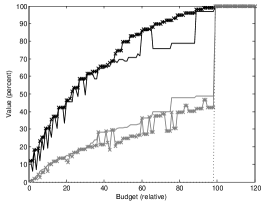
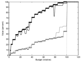
The results of our simulations also showed (Figure 3) that the efficiency of the BKP-PC model was severely impacted by the selection deficiency problem (SDP). In other words, the BKP-PC model generated the lowest $AV/OV$ unless in the presence of a sufficient budget ( $Budget\to 120$ ) and/or a negligible level of interdependency ( $LOI\to 0$ ).

For $LOI>0.25$ in both RAN and PMR requirement sets, almost no $AV/OV$ was achieved by the BKP-PC model unless budget was available for all of the requirements ( $b=\sum_{i=1}^{14}c_{i}=99$ for the RAN). It was moreover, observed (Figure 3) that the GORS model mitigated the impact of the SDP through considering the strengths of value-related dependencies.

The BKP model however was not subject to the SDP as it completely ignored dependencies among requirements.

We further observed (Figure 3) that all the of the selection models performed similar when budget was available for all of the requirements to be implemented ( $Budget\geq 99$ for RAN and $Budget\geq$ 101 for PMR) or requirements were mutually independent.

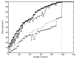
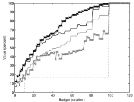
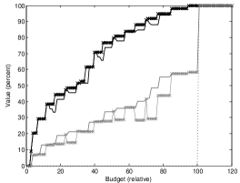
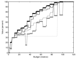
Figure 4 and Figure 5 compare AV/OV achieved by the simulated selection models for various levels of interdependencies among requirements of the RAN and PMR respectively. A dependency level of $LOI=0.8$ implies that $80\%$ of the explicit value-related dependencies have non-zero strengths. The horizontal axis shows the available budget and the vertical axis shows the percentage of the achieved $AV/OV$ .

In almost every simulation, it was observed that for a given optimal set $O$ , AV of $O$ was smaller or equal to the OV of $O$ . This is due to the fact that the overall value of an optimal set considers the impacts of value-related dependencies among requirements whereas the accumulated value of an optimal set accumulates the estimated values of selected requirements without considering their value-related dependencies.

It was further observed that the gap between overall value of an optimal set and its corresponding accumulated value ( $|AV-OV|$ ) increased as the level of interdependency (LOI) grew. The reason is that increasing the LOI increases the chances that selected requirements explicitly depend on the excluded requirements which generally results in decreasing the of overall value of the optimal set.

The BKP-PC model however always avoids choosing a requirement without its dependencies being selected. In other words, the BKP-PC model avoids dependencies from the optimal set to the excluded set and as such $AV=OV$ always holds for the BKP-PC models.

5.2 Case Study

To demonstrate practicality of the GORS model, we performed selection for $23$ requirements of a messaging software referred to as the Precious Messaging System (PMS). We employed $5$ stakeholders to estimate greer_software_2004 the costs and values of requirements of the PMS. Each requirement $r_{i}$ was assigned an estimated cost of $c_{i}\in[1,20]$ and an estimated value of $v_{i}\in[1,20]$ by different stakeholders.

Stakeholders then, performed pairwise comparisons among requirements carlshamre_industrial_2001 to identify explicit value-related dependencies and estimate the strengths of those dependencies. A dependency $(r_{i},r_{j})$ was assigned an strength of $\rho(r_{i},r_{j})\in[0,1]$ where $\rho(r_{i},r_{j})=0$ and $\rho(r_{i},r_{j})=1$ denoted no dependency and a full dependency from $r_{i}$ to $r_{j}$ respectively.

The median of $5$ estimated costs/values for each requirement $r_{i}$ then was computed to account for different opinions of stakeholders. In a similar way, for each explicit value-related dependency $(r_{i},r_{j})$ the median of the $5$ estimated strengths of that dependency was computed to specify the strength of $(r_{i},r_{j})$ . Median was taken as the measure of central tendency as it is less affected by (potentially) extreme opinions of stakeholders compared to the arithmetic mean.

Table 4 lists the estimated costs and values of the requirement of the PMS as well as the strengths of explicit value-related dependencies among those requirements. The Dependency Vector of a requirement $r_{i}$ in Table 4 denotes the strengths of explicit value-related dependencies from $r_{i}$ to other requirements of the PMS. Based on Table 4 and (7), level of interdependency is calculated for the requirements of the PMS as follows. $LOI(PMS)=\frac{113}{{{}^{23}\mkern-3.0muP_{2}}}\approxeq 0.22$ .

Table 4: Estimated values, costs, and strengths of explicit value-related dependencies (based on stakeholder’s estimations).

ID	Value	Cost	Dependency Vector $\{r_{1},...,r_{23}\}$

$r_{1}$	$20$	$10$	$\{0.0,0.0,0.0,0.5,0.3,0.0,0.6,0.4,0.0,0.0,0.0,0.7,0.0,0.0,0.0,0.0,0.0,0.0,0.0,0.0,0.1,0.0,0.3\}$
$r_{2}$	$20$	$7$	$\{1.0,0.0,0.0,0.6,0.6,0.0,0.6,0.6,0.0,0.3,0.3,0.7,0.0,0.3,0.0,0.7,0.0,0.0,0.0,0.0,0.2,0.0,0.8\}$
$r_{3}$	$6$	$1$	$\{1.0,0.0,0.0,0.5,0.3,0.0,0.6,0.0,0.0,0.0,0.0,0.7,0.0,0.0,0.0,0.0,0.0,0.0,0.0,0.0,0.0,0.0,0.0\}$
$r_{4}$	$17$	$10$	$\{0.0,0.0,0.0,0.0,0.0,0.0,0.0,0.0,0.0,0.0,0.9,0.0,0.0,0.4,0.0,0.7,0.0,0.0,0.0,0.0,0.2,0.0,0.0\}$
$r_{5}$	$3$	$12$	$\{0.0,0.0,0.0,0.0,0.0,0.0,0.0,0.0,0.0,0.0,0.5,0.0,0.0,0.0,0.0,0.2,0.0,0.0,0.0,0.0,0.0,0.0,0.0\}$
$r_{6}$	$20$	$20$	$\{0.0,0.0,0.0,0.0,0.0,0.0,0.6,0.0,0.3,0.3,0.4,0.0,0.0,0.0,0.0,0.7,0.4,0.0,0.0,0.0,0.0,0.0,0.8\}$
$r_{7}$	$15$	$6$	$\{0.0,0.0,0.0,0.0,0.0,0.0,0.0,0.0,0.0,0.0,0.0,0.0,0.0,0.0,0.0,0.0,0.0,0.0,0.0,0.0,0.0,0.0,0.0\}$
$r_{8}$	$8$	$14$	$\{0.0,0.0,0.0,0.0,0.0,0.0,0.0,0.0,0.0,0.0,0.4,0.0,0.0,0.0,0.0,0.0,0.0,0.0,0.0,0.0,0.0,0.0,0.0\}$
$r_{9}$	$20$	$15$	$\{0.0,0.7,0.0,0.0,0.0,0.7,0.0,0.3,0.0,0.0,0.8,0.2,0.4,0.0,0.2,0.7,0.0,0.0,0.0,0.0,0.2,0.0,0.0\}$
$r_{10}$	$16$	$10$	$\{0.0,0.7,0.0,0.0,0.3,0.7,0.0,0.3,0.0,0.0,0.0,0.3,0.4,0.0,0.0,0.2,0.0,0.0,0.0,0.0,0.2,0.6,0.0\}$
$r_{11}$	$20$	$4$	$\{0.0,0.0,0.0,0.4,0.0,0.0,0.0,0.0,0.0,0.0,0.0,0.0,0.0,0.0,0.0,0.0,0.4,0.0,0.0,0.0,0.2,0.0,0.0\}$
$r_{12}$	$10$	$6$	$\{0.0,0.0,0.0,0.0,0.0,0.0,0.0,0.0,0.5,0.5,0.8,0.0,0.0,0.0,0.1,0.4,0.0,0.0,0.0,0.0,0.0,0.4,0.0\}$
$r_{13}$	$8$	$5$	$\{0.0,0.0,0.0,0.0,0.0,0.0,0.0,0.0,0.0,0.0,0.8,0.0,0.0,0.0,0.1,0.4,0.0,0.0,0.0,0.0,0.1,0.6,0.0\}$
$r_{14}$	$5$	$12$	$\{0.0,0.0,0.0,0.0,0.0,0.0,0.0,0.0,0.0,0.0,0.8,0.0,0.0,0.0,0.0,0.8,0.0,0.0,0.0,0.0,0.8,0.0,0.0\}$
$r_{15}$	$8$	$15$	$\{0.0,0.0,0.0,0.0,0.0,0.0,0.0,0.0,0.0,0.0,0.8,0.0,0.0,0.0,0.0,0.8,0.0,0.0,0.0,0.0,1.0,0.0,0.0\}$
$r_{16}$	$10$	$3$	$\{0.0,0.0,0.0,0.0,0.0,0.0,0.0,0.0,0.0,0.0,0.8,0.0,0.0,0.0,0.0,0.0,0.5,0.0,0.0,0.0,0.0,0.0,0.0\}$
$r_{17}$	$15$	$12$	$\{0.0,0.0,0.0,0.0,0.0,0.0,0.0,0.0,0.0,0.0,0.8,0.0,0.0,0.0,0.0,0.0,0.0,0.5,0.0,0.0,0.0,0.0,0.0\}$
$r_{18}$	$10$	$3$	$\{0.0,0.0,0.0,0.0,0.0,0.0,0.0,0.0,0.0,0.0,0.0,0.0,0.0,0.0,0.0,0.0,0.0,0.0,0.0,0.0,0.0,0.0,0.0\}$
$r_{19}$	$20$	$20$	$\{1.0,0.3,0.0,0.7,0.5,1.0,0.6,0.5,1.0,0.6,0.4,0.0,0.0,0.1,0.8,0.8,0.0,0.0,0.0,0.0,0.0,0.0,0.8\}$
$r_{20}$	$20$	$20$	$\{1.0,0.3,0.0,0.7,0.5,1.0,0.6,0.5,1.0,0.6,0.4,0.0,0.0,0.1,0.8,0.8,0.0,0.0,0.0,0.0,0.0,0.0,0.8\}$
$r_{21}$	$15$	$12$	$\{0.0,0.0,0.0,0.0,0.0,0.0,0.0,0.0,0.0,0.0,0.8,0.0,0.0,0.0,0.1,0.8,0.2,0.0,0.0,0.0,0.0,0.3,0.0\}$
$r_{22}$	$20$	$15$	$\{0.0,0.0,0.0,0.0,0.0,0.0,0.0,0.0,0.0,0.0,0.0,0.0,0.0,0.0,0.0,0.0,0.0,0.0,0.0,0.0,0.0,0.0,0.0\}$
$r_{23}$	$20$	$10$	$\{0.0,0.0,0.0,0.0,0.0,0.0,0.0,0.0,0.0,0.0,0.0,0.0,0.0,0.0,0.0,0.0,0.0,0.0,0.0,0.0,0.0,0.0,0.0\}$

Table 5: Solution vectors and their corresponding overall value (OV) provided by the experimented selection models in the presence of various budget constraints. A selection variable

x_{i}

denotes whether requirement

r_{i}

is selected (

x_{i}=1

) or otherwise (

x_{i}=0

)

Budget	Selection Model	Overall Value (percent)	Solution Vector $\{x_{1},...,x_{23}\}$
16	BKP	5.21	$\{0,1,1,0,0,0,0,0,0,0,1,0,0,0,0,1,0,0,0,0,0,0,0\}$
	BKP-PC	10.74	$\{0,0,0,0,0,0,1,0,0,0,0,0,0,0,0,0,0,0,0,0,0,0,1\}$
	GORS	12.88	$\{0,0,0,0,0,0,1,0,0,0,1,0,0,0,0,1,0,1,0,0,0,0,0\}$ \bigstrut[b]
46	BKP	23.25	$\{1,1,1,0,0,0,1,0,0,0,1,0,0,0,0,1,0,1,0,0,0,0,1\}$ \bigstrut[t]
	BKP-PC	19.94	$\{0,0,0,0,0,0,1,0,0,0,0,0,0,0,0,0,0,1,0,0,0,1,1\}$
	GORS	26.63	$\{0,0,0,0,0,0,1,0,0,0,1,0,1,0,0,1,0,1,0,0,0,1,1\}$ \bigstrut[b]
71	BKP	31.07	$\{1,1,1,1,0,0,1,0,0,1,1,1,0,0,0,1,0,1,0,0,0,0,1\}$ \bigstrut[t]
	BKP-PC	19.94	$\{0,0,0,0,0,0,1,0,0,0,0,0,0,0,0,0,0,1,0,0,0,1,1\}$
	GORS	34.60	$\{1,1,1,0,0,0,1,0,0,0,1,1,1,0,0,1,0,1,0,0,0,1,1\}$ \bigstrut[b]
76	BKP	32.06	$\{1,1,1,1,0,0,1,0,0,1,1,1,1,0,0,1,0,1,0,0,0,0,1\}$ \bigstrut[t]
	BKP-PC	19.94	$\{0,0,0,0,0,0,1,0,0,0,0,0,0,0,0,0,0,1,0,0,0,1,1\}$
	GORS	35.74	$\{1,1,1,1,0,0,1,0,0,0,1,1,0,0,0,1,0,1,0,0,0,1,1\}$ \bigstrut[b]
81	BKP	31.90	$\{1,1,1,1,0,0,1,0,0,1,1,0,1,0,0,1,1,1,0,0,0,0,1\}$ \bigstrut[t]
	BKP-PC	19.94	$\{0,0,0,0,0,0,1,0,0,0,0,0,0,0,0,0,0,1,0,0,0,1,1\}$
	GORS	37.98	$\{0,0,0,1,0,0,0,0,0,0,1,0,0,1,0,1,1,1,0,0,1,1,1\}$ \bigstrut[b]
141	BKP	44.11	$\{1,1,1,1,0,0,1,0,1,1,1,1,1,0,0,1,1,1,0,1,0,1,1\}$ \bigstrut[t]
	BKP-PC	53.37	$\{0,0,0,1,1,0,1,1,0,0,1,0,1,1,1,1,1,1,0,0,1,1,1\}$
	GORS	59.45	$\{1,1,1,1,0,0,1,0,0,1,1,1,1,1,1,1,1,1,0,0,1,1,1\}$ \bigstrut[b]
146	BKP	45.40	$\{1,1,1,1,0,0,1,0,1,1,1,1,0,0,0,1,1,1,0,1,1,1,1\}$ \bigstrut[t]
	BKP-PC	53.37	$\{0,0,0,1,1,0,1,1,0,0,1,0,1,1,1,1,1,1,0,0,1,1,1\}$
	GORS	60.43	$\{1,1,1,1,0,0,1,1,0,0,1,1,1,1,1,1,1,1,0,0,1,1,1\}$ \bigstrut[b]
151	BKP	46.87	$\{1,1,1,1,0,0,1,0,1,1,1,1,1,0,0,1,1,1,0,1,1,1,1\}$ \bigstrut[t]
	BKP-PC	53.37	$\{0,0,0,1,1,0,1,1,0,0,1,0,1,1,1,1,1,1,0,0,1,1,1\}$
	GORS	62.27	$\{1,1,1,1,0,1,1,0,0,0,1,1,1,1,1,1,1,1,0,0,1,1,1\}$ \bigstrut[b]
156	BKP	46.87	$\{1,1,1,1,0,0,1,0,1,1,1,1,1,0,0,1,1,1,0,1,1,1,1\}$ \bigstrut[t]
	BKP-PC	53.37	$\{0,0,0,1,1,0,1,1,0,0,1,0,1,1,1,1,1,1,0,0,1,1,1\}$
	GORS	62.27	$\{1,1,1,1,0,1,1,0,0,0,1,1,1,1,1,1,1,1,0,0,1,1,1\}$ \bigstrut[b]
161	BKP	50.12	$\{1,1,1,1,0,1,1,0,1,1,1,1,1,0,0,1,1,1,0,1,0,1,1\}$ \bigstrut[t]
	BKP-PC	53.37	$\{0,0,0,1,1,0,1,1,0,0,1,0,1,1,1,1,1,1,0,0,1,1,1\}$
	GORS	64.23	$\{1,1,1,1,0,1,1,0,0,1,1,1,1,1,1,1,1,1,0,0,1,1,1\}$ \bigstrut[b]
166	BKP	51.41	$\{1,1,1,1,0,1,1,0,1,1,1,1,0,0,0,1,1,1,0,1,1,1,1\}$ \bigstrut[t]
	BKP-PC	53.37	$\{0,0,0,1,1,0,1,1,0,0,1,0,1,1,1,1,1,1,0,0,1,1,1\}$
	GORS	64.72	$\{1,1,1,1,0,1,1,0,1,0,1,1,1,1,1,1,1,1,0,0,1,1,1\}$ \bigstrut[b]
171	BKP	52.88	$\{1,1,1,1,0,1,1,0,1,1,1,1,1,0,0,1,1,1,0,1,1,1,1\}$ \bigstrut[t]
	BKP-PC	53.37	$\{0,0,0,1,1,0,1,1,0,0,1,0,1,1,1,1,1,1,0,0,1,1,1\}$
	GORS	64.72	$\{1,1,1,1,0,1,1,0,1,0,1,1,1,1,1,1,1,1,0,0,1,1,1\}$ \bigstrut[b]
176	BKP	52.88	$\{1,1,1,1,0,1,1,0,1,1,1,1,1,0,0,1,1,1,0,1,1,1,1\}$ \bigstrut[t]
	BKP-PC	53.37	$\{0,0,0,1,1,0,1,1,0,0,1,0,1,1,1,1,1,1,0,0,1,1,1\}$
	GORS	66.69	$\{1,1,1,1,0,1,1,1,0,1,1,1,1,1,1,1,1,1,0,0,1,1,1\}$ \bigstrut[b]
181	BKP	51.35	$\{1,1,1,1,0,1,1,0,1,1,1,1,1,0,0,1,1,1,1,1,0,1,1\}$ \bigstrut[t]
	BKP-PC	53.37	$\{0,0,0,1,1,0,1,1,0,0,1,0,1,1,1,1,1,1,0,0,1,1,1\}$
	GORS	67.18	$\{1,1,1,1,0,1,1,1,1,0,1,1,1,1,1,1,1,1,0,0,1,1,1\}$ \bigstrut[b]
186	BKP	52.64	$\{1,1,1,1,0,1,1,0,1,1,1,1,0,0,0,1,1,1,1,1,1,1,1\}$ \bigstrut[t]
	BKP-PC	53.37	$\{0,0,0,1,1,0,1,1,0,0,1,0,1,1,1,1,1,1,0,0,1,1,1\}$
	GORS	73.83	$\{1,1,0,1,1,1,1,1,1,1,1,1,1,1,0,1,1,1,0,0,1,1,1\}$ \bigstrut[b]
191	BKP	54.11	$\{1,1,1,1,0,1,1,0,1,1,1,1,1,0,0,1,1,1,1,1,1,1,1\}$ \bigstrut[t]
	BKP-PC	53.37	$\{0,0,0,1,1,0,1,1,0,0,1,0,1,1,1,1,1,1,0,0,1,1,1\}$
	GORS	75.31	$\{1,1,1,1,1,1,1,1,1,1,1,1,1,1,0,1,1,1,0,0,1,1,1\}$ \bigstrut[b]
196	BKP	54.11	$\{1,1,1,1,0,1,1,0,1,1,1,1,1,0,0,1,1,1,1,1,1,1,1\}$ \bigstrut[t]
	BKP-PC	53.37	$\{0,0,0,1,1,0,1,1,0,0,1,0,1,1,1,1,1,1,0,0,1,1,1\}$
	GORS	75.31	$\{1,1,1,1,1,1,1,1,1,1,1,1,1,1,0,1,1,1,0,0,1,1,1\}$ \bigstrut[b]
246	BKP	100.00	$\{1,1,1,1,1,1,1,1,1,1,1,1,1,1,1,1,1,1,1,1,1,1,1\}$ \bigstrut[t]
	BKP-PC	100.00	$\{1,1,1,1,1,1,1,1,1,1,1,1,1,1,1,1,1,1,1,1,1,1,1\}$
	GORS	100.00	$\{1,1,1,1,1,1,1,1,1,1,1,1,1,1,1,1,1,1,1,1,1,1,1\}$

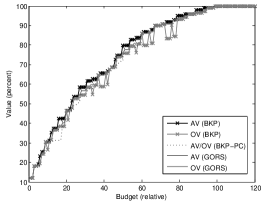
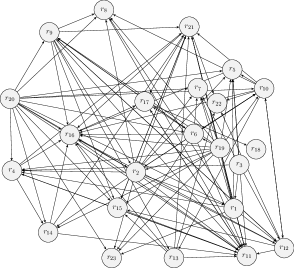
Based on the estimations provided by the stakeholders, FRIG of the PMS was constructed (Figure 6) and selections were performed using the GORS model as well as the BKP and BKP-PC models. Requirement selections were performed for various ranges of budgets ( $Budget\in\{1,...,260\}$ ) to examine the performance of the selection models.

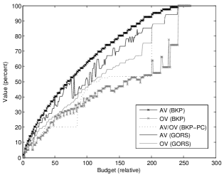
Figure 7 summarizes the results of our experiments by comparing the accumulated values (AV) and/or overall values (OV) achieved by the selection models. The horizontal axis shows the available budget ( $Budget=\{1,...,260\}$ ) and the vertical axis shows the percentages of $AV/OV$ . Table 5 lists some of the optimal sets provided by the employed selection models in the presence of various budget constraints.

Consistent with the simulations, the results of our case study demonstrated (Figure 7 and Table 5) that the BKP model always maximized the accumulated value of the selected requirements (optimal set) while the GORS model maximized the overall value of selected requirements. Moreover, maximizing accumulated value and overall value of an optimal set demonstrated to be conflicting objectives.

Furthermore, the results of our experiments showed (Figure 7 and Table 5) that the GORS model mitigated the adverse impact of the selection deficiency problem (SDP) through considering the strengths of value-related requirement dependencies while the efficiency of the BKP-PC model was negatively impacted by the SDP. For instance, we observed (Table 5) that for $Budget=81$ , overall value of the optimal set provided by the GORS model was almost twice as higher as the overall value provided by the BKP-PC model. The BKP model on the contrary, was not vulnerable to the SDP as it totally ignores dependencies.

6 Automated Identification of Explicit Value-related Requirement Dependencies

Automated identification of value-related requirement dependencies and their strengths has not been discussed in the existing literature. Nonetheless, various techniques from information retrieval and data mining domain Halpern01062015 can be borrowed to assist such automation.

This section discusses one of the several possible approaches to automate identification of value-related requirement dependencies. Our proposed approach is based on mining preferences of (potential) users of a software do2016incorporating to identify both the existence and the strengths of explicit value-related dependencies among requirements of a software.

It has been widely recognize in the literature that users’ preferences (customers’ preferences) of software requirements can determine their customer values do2016incorporating ; racheva_business_2010 as highly preferred software requirements are more likely to be purchased and used by the (potential) users. On the other hand, users preferring a requirement $r_{j}$ may also prefer a requirement $r_{i}$ (with the probability $p(r_{i}|r_{j})$ ). This is known as Market Basket Analysis or Association Rule Mining in data mining domain Halpern01062015 .

An association from a requirement $r_{j}$ to $r_{i}$ (users preferring $r_{j}$ will also prefer $r_{i}$ ) can also be interpreted as a causal relation sprenger2016foundations from $r_{j}$ to $r_{i}$ meaning that preference (selection) of $r_{j}$ may cause preference of $r_{i}$ by the users and therefore give the value of $r_{i}$ . As such, it is clear that a causal relation from $r_{j}$ to $r_{i}$ also can be interpreted as a value-related dependency from $r_{i}$ to $r_{j}$ (value of $r_{i}$ depends on preference of $r_{j}$ by the users).

Hence, association rule mining of users’ preference of requirements can be used for identification of value-related requirement dependencies and the strengths of those dependencies. In this context, measures of causal strength can be used to estimate the strengths of value-related dependencies.

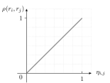
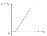
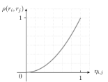
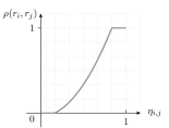
One of the most commonly adopted measures of causal strength is Pearl’s Measure of Causal Strength sprenger2016foundations ; Halpern01062015 ; pearl2009causality ; janzing2013quantifying ; eells1991probabilistic which is denoted by $\eta$ _i,j in $(\ref{Eq_Pearl})$ and derived by $p(r_{i}|r_{j})$ . That is the chances that users preferring $r_{j}$ will also prefer $r_{i}$ . This can be used to estimate the strength of an explicit value-related dependency from $r_{i}$ to $r_{j}$ . Pearl’s measure then can be mapped into a desired fuzzy membership function $\rho(r_{i},r_{j})$ (which gives the strengths of value-related dependencies in FRIGs) as demonstrated in Figure 7(e).

Various membership functions could be explored for this mapping based on the preference of the analyst. For instance, the membership function of Figure 6 treats dependencies with casual strengths below $0.16$ ( $\eta_{i,j}<0.16$ ) as not worth considering while dependencies with $\eta_{i,j}\geq 0.83$ are treated as full dependencies of strength $1$ . Such membership function might be suitable for selection models that formulate dependencies as precedence constraints (BKP-PC models).

In such models, it might be reasonable to consider a strong causal dependency (say $\eta_{i,j}\geq 0.95$ ) as a precedence relation rather than ignoring it (BKP-PC models only capture precedence relations). Figure 6 and Figure 7(e) depict other alternative membership functions which unlike membership functions of Figure 6 and Figure 6 do not assume linearity for mapping $\eta_{i,j}$ to $\rho(r_{i},r_{j})$ .

\displaystyle\phantom{ssssss}\eta_{i,j}=p(r_{i}|r_{j})=\frac{p(r_{i},r_{j})}{p(r_{j})},\phantom{s}\eta_{i,j}\in[0,1]

(12)

References

- (1) A. J. Bagnall, V. J. RaywardSmith, and I. M. Whittley, “The next release problem,” Information and Software Technology, vol. 43, no. 14, pp. 883–890, Dec. 2001.
- (2) D. Mougouei, D. M. Powers, and E. Mougouei, “A fuzzy framework for prioritization and partial selection of security requirements in software projects,” Journal of Intelligent & Fuzzy Systems, no. Preprint, pp. 1–17, 2019.
- (3) D. Mougouei, H. Shen, and M. A. Babar, “Partial selection of agile software requirements,” International Journal of Software Engineering and Its Applications, vol. 9, no. 01, pp. 113–126, 2015.
- (4) A. G. Dahlstedt and A. Persson, “Requirements interdependencies - moulding the state of research into a research agenda,” in Ninth International Workshop on Requirements Engineering: Foundation for Software Quality (REFSQ 2003), 2003, pp. 71–80.
- (5) S. Barney, A. Aurum, and C. Wohlin, “A product management challenge: Creating software product value through requirements selection,” Journal of Systems Architecture, vol. 54, no. 6, pp. 576–593, Jun. 2008.
- (6) G. Ruhe, Product Release Planning: Methods, Tools and Applications. Taylor & Francis, Jun. 2010.
- (7) P. Achimugu, A. Selamat, R. Ibrahim, and M. N. Mahrin, “A systematic literature review of software requirements prioritization research,” Information and Software Technology, vol. 56, no. 6, pp. 568–585, Jun. 2014.
- (8) N. Kukreja, S. S. Payyavula, B. Boehm, and S. Padmanabhuni, “Value-based requirements prioritization: Usage experiences,” Procedia Computer Science, vol. 16, pp. 806–813, 2013.
- (9) N. D. Fogelström, E. Numminen, and S. Barney, “Using portfolio theory to support requirements selection decisions,” in 2010 Fourth International Workshop on Software Product Management. IEEE, 2010, pp. 49–52.
- (10) D. Mougouei, D. M. W. Powers, and A. Moeini, “An integer linear programming model for binary knapsack problem with dependent item values,” in AI 2017: Advances in Artificial Intelligence: 30th Australasian Joint Conference, Melbourne, VIC, Australia, August 19–20, 2017, Proceedings, vol. 10400. Springer International Publishing, 2017, pp. 144–154.
- (11) M. Harman, J. Krinke, I. MedinaBulo, F. PalomoLozano, J. Ren, and S. Yoo, “Exact scalable sensitivity analysis for the next release problem,” ACM Trans. Softw. Eng. Methodol., vol. 23, no. 2, p. 19:1–19:31, Apr. 2014. [Online]. Available: http://doi.acm.org/10.1145/2537853
- (12) Ákos Szőke, “Conceptual scheduling model and optimized release scheduling for agile environments,” Information and Software Technology, vol. 53, no. 6, pp. 574–591, Jun. 2011.
- (13) Y. Zhang, M. Harman, and S. A. Mansouri, “The multi-objective next release problem,” in Proceedings of the 9th Annual Conference on Genetic and Evolutionary Computation. New York, NY, USA: ACM, 2007, p. 1129–1137.
- (14) P. Carlshamre, “Release planning in market-driven software product development: Provoking an understanding,” Requirements Engineering, vol. 7, no. 3, pp. 139–151, Sep. 2002.
- (15) T. Lust and J. Teghem, “The multiobjective multidimensional knapsack problem: a survey and a new approach,” International Transactions in Operational Research, vol. 19, no. 4, p. 495–520, 2012.
- (16) J. Karlsson and K. Ryan, “A costvalue approach for prioritizing requirements,” IEEE Software, vol. 14, no. 5, pp. 67–74, Sep. 1997.
- (17) H.-W. Jung, “Optimizing value and cost in requirements analysis,” IEEE Software, vol. 15, no. 4, pp. 74–78, Jul. 1998.
- (18) M. van den Akker, S. Brinkkemper, G. van Diepen, and J. Versendaal, “Flexible release planning using integer linear programming,” REFSQ’05, 2005.
- (19) D. Mougouei, “Factoring requirement dependencies in software requirement selection using graphs and integer programming,” in Proceedings of the 31st IEEE/ACM International Conference on Automated Software Engineering. ACM, 2016, pp. 884–887.
- (20) D. Mougouei and D. M. Powers, “Dependency-aware software release planning through mining user preferences,” Soft Computing, 2020.
- (21) ——, “Dependency-aware release planning for software projects using fuzzy graphs and integer programming,” Journal of Intelligent & Fuzzy Systems, pp. 1–15, 2019.
- (22) D. Mougouei, “A mathematical programming approach to considering value dependencies in software requirement selection (thesis),” Ph.D. dissertation, Flinders University, School of Computer Science, Engineering and Mathematics., 2018.
- (23) D. Mougouei, D. M. Powers, and A. Moeini, “Dependency-aware software release planning,” in 2017 IEEE/ACM 39th International Conference on Software Engineering Companion (ICSE-C). IEEE, 2017, pp. 198–200.
- (24) D. Mougouei and D. M. Powers, “Modeling and selection of interdependent software requirements using fuzzy graphs,” International Journal of Fuzzy Systems, pp. 1–17, 2017.
- (25) Å. G. Dahlstedt and A. Persson, “Requirements interdependencies: state of the art and future challenges,” in Engineering and managing software requirements. Springer, 2005, pp. 95–116.
- (26) J. Karlsson, S. Olsson, and K. Ryan, “Improved practical support for largescale requirements prioritising,” Requirements Engineering, vol. 2, no. 1, pp. 51–60, Mar. 1997.
- (27) W. N. Robinson, S. D. Pawlowski, and V. Volkov, “Requirements interaction management,” ACM Comput. Surv., vol. 35, no. 2, pp. 132-190, Jun. 2003.
- (28) B. Ramesh and M. Jarke, “Toward reference models for requirements traceability,” IEEE Transactions on Software Engineering, vol. 27, no. 1, pp. 58–93, Jan. 2001.
- (29) J. Wang, J. Li, Q. Wang, H. Zhang, and H. Wang, “A simulation approach for impact analysis of requirement volatility considering dependency change,” in Requirements Engineering: Foundation for Software Quality, B. Regnell and D. Damian, Eds. Springer Berlin Heidelberg, Jan. 2012, no. 7195, pp. 59–76.
- (30) M. M. A. Brasil, T. G. N. d. Silva, F. G. d. Freitas, J. T. d. Souza, and M. I. Cortés, “A multiobjective optimization approach to the software release planning with undefined number of releases and interdependent requirements,” in Enterprise Information Systems, R. Zhang, J. Zhang, Z. Zhang, J. Filipe, and J. Cordeiro, Eds. Springer Berlin Heidelberg, Jan. 2012, no. 102, pp. 300–314.
- (31) A. Finkelstein, M. Harman, S. A. Mansouri, J. Ren, and Y. Zhang, “A search based approach to fairness analysis in requirement assignments to aid negotiation, mediation and decision making,” Requirements Engineering, vol. 14, no. 4, pp. 231–245, 2009.
- (32) J. del Sagrado, I. M. del Aguila, and F. J. Orellana, “Ant colony optimization for the next release problem: A comparative study,” in Search Based Software Engineering (SSBSE), 2010 Second International Symposium on. IEEE, 2010, pp. 67–76.
- (33) L. Li, M. Harman, F. Wu, and Y. Zhang, “The value of exact analysis in requirements selection,” IEEE Transactions on Software Engineering, 2016.
- (34) N. Veerapen, G. Ochoa, M. Harman, and E. K. Burke, “An integer linear programming approach to the single and bi-objective next release problem,” Information and Software Technology, vol. 65, pp. 1–13, 2015.
- (35) D. Greer and G. Ruhe, “Software release planning: an evolutionary and iterative approach,” vol. 46, no. 4, pp. 243–253, 2004.
- (36) G. Ruhe and D. Greer, “Quantitative studies in software release planning under risk and resource constraints,” in Proceedings of the 2003 International Symposium on Empirical Software Engineering, Sept 2003, pp. 262–270.
- (37) G. van Valkenhoef, T. Tervonen, B. de Brock, and D. Postmus, “Quantitative release planning in extreme programming,” Information and software technology, vol. 53, no. 11, pp. 1227–1235, 2011.
- (38) Y. Zhang and M. Harman, “Search based optimization of requirements interaction management,” in Search Based Software Engineering (SSBSE), 2010 Second International Symposium on. IEEE, 2010, pp. 47–56.
- (39) M. O. Saliu and G. Ruhe, “Bi-objective release planning for evolving software systems,” in Proceedings of the the 6th joint meeting of the European software engineering conference and the ACM SIGSOFT symposium on The foundations of software engineering. ACM, 2007, pp. 105–114.
- (40) M. van den Akker, S. Brinkkemper, G. Diepen, and J. Versendaal, “Determination of the next release of a software product: an approach using integer linear programming.” in CAiSE Short Paper Proceedings, 2005.
- (41) A. Ngo-The and G. Ruhe, “Optimized resource allocation for software release planning,” IEEE Transactions on Software Engineering, vol. 35, no. 1, pp. 109–123, 2009.
- (42) W.-N. Chen and J. Zhang, “Ant colony optimization for software project scheduling and staffing with an event-based scheduler,” IEEE Transactions on Software Engineering, vol. 39, no. 1, pp. 1–17, 2013.
- (43) J. Xuan, H. Jiang, Z. Ren, and Z. Luo, “Solving the large scale next release problem with a backbone-based multilevel algorithm,” IEEE Transactions on Software Engineering, vol. 38, no. 5, pp. 1195–1212, 2012.
- (44) M. van den Akker, S. Brinkkemper, G. Diepen, and J. Versendaal, “Software product release planning through optimization and what-if analysis,” Information and Software Technology, vol. 50, no. 1, pp. 101–111, 2008.
- (45) C. Li, M. v. d. Akker, S. Brinkkemper, and G. Diepen, “An integrated approach for requirement selection and scheduling in software release planning,” Requirements Engineering, vol. 15, no. 4, pp. 375–396, Nov. 2010.
- (46) A. Kalampakas, S. Spartalis, L. Iliadis, and E. Pimenidis, “Fuzzy graphs: algebraic structure and syntactic recognition,” Artificial Intelligence Review, pp. 1–12, Jul. 2013.
- (47) H.-J. Zimmermann, “Fuzzy relations and fuzzy graphs,” in Fuzzy Set Theory and Its Applications. Springer Netherlands, Jan. 1996, pp. 69–89.
- (48) A. Rosenfeld, “Fuzzy graphs,” Fuzzy Sets and Their Applications, vol. 77, p. 95, 1975.
- (49) J. N. Mordeson, “Fuzzy mathematics,” in Foundations of Image Understanding, L. S. Davis, Ed. Springer US, Jan. 2001, no. 628, pp. 95–125.
- (50) B. Korte and J. Vygen, Combinatorial Optimization: Theory and Algorithms. Springer, 2006.
- (51) P. Carlshamre, K. Sandahl, M. Lindvall, B. Regnell, and J. Natt och Dag, “An industrial survey of requirements interdependencies in software product release planning,” in Fifth IEEE International Symposium on Requirements Engineering, 2001. Proceedings, 2001, pp. 84–91.
- (52) G. Ruhe, A. Eberlein, and D. Pfahl, “Trade-off analysis for requirements selection,” International Journal of Software Engineering and Knowledge Engineering, vol. 13, no. 04, pp. 345-366, 2003.
- (53) J. d. Sagrado, I. M. d. Águila, and F. J. Orellana, “Multiobjective ant colony optimization for requirements selection,” Empirical Software Engineering, pp. 1–34, Nov. 2013.
- (54) Y. Zhang, M. Harman, and S. L. Lim, “Empirical evaluation of search based requirements interaction management,” Information and Software Technology, vol. 55, no. 1, pp. 126 – 152, 2013, special section: Best papers from the 2nd International Symposium on Search Based Software Engineering 2010.
- (55) A. NgoThe and M. Saliu, “Fuzzy structural dependency constraints in software release planning,” in Fuzzy Systems, 2005. FUZZ ’05. The 14th IEEE International Conference on, May 2005, pp. 442-447.
- (56) S. Mathew and M. Sunitha, “Strongest strong cycles and theta fuzzy graphs,” Fuzzy Systems, IEEE Transactions on, vol. 21, no. 6, pp. 1096-1104, Dec 2013.
- (57) J. N. Mordeson and P. S. Nair, “Applications of fuzzy graphs,” in Fuzzy Graphs and Fuzzy Hypergraphs, J. N. Mordeson and P. S. Nair, Eds. PhysicaVerlag HD, Jan. 2000, no. 46, pp. 83–133.
- (58) D. Mougouei and W. Nurhayati, “A fuzzy-based technique for describing security requirements of intrusion tolerant systems,” International Journal of Software Engineering and its Applications, vol. 7, no. 2, pp. 99–112, 2013.
- (59) D. Mougouei, W. Rahman, and M. M. Almasi, “Measuring security of web services in requirement engineering phase,” International Journal of Cyber-Security and Digital Forensics (IJCSDF), vol. 1, no. 2, pp. 89–98, 2012.
- (60) D. Mougouei, M. Moghtadaei, and S. Moradmand, “A goal-based modeling approach to develop security requirements of fault tolerant security-critical systems,” in 2012 International Conference on Computer and Communication Engineering (ICCCE). IEEE, 2012, pp. 200–205.
- (61) L. A. Zadeh, “Fyzzy sets,” Inf. Comput., vol. 8, pp. 338-353, Dec 1965.
- (62) G. J. Klir and T. A. Folger, Fuzzy Sets, Uncertainty, and Information. Upper Saddle River, NJ, USA: Prentice-Hall, Inc., 1987.
- (63) J. Karlsson and K. Ryan, “Supporting the selection of software requirements,” in Software Specification and Design, 1996., Proceedings of the 8th International Workshop on, Mar 1996, pp. 146–149.
- (64) A. M. Law and W. D. Kelton, Simulation Modeling and Analysis, 2nd ed. McGraw-Hill Higher Education, 1997.
- (65) “Random (Java Platform SE 7 ).” [Online]. Available: http://docs.oracle.com/javase/7/docs/api/java/util/Random.html
- (66) J. Y. Halpern and C. Hitchcock, “Graded causation and defaults,” The British Journal for the Philosophy of Science, vol. 66, no. 2, pp. 413–457, 2015. [Online]. Available: http://bjps.oxfordjournals.org/content/66/2/413.abstract
- (67) T. do Nascimento Ferreira, A. A. Araújo, A. D. B. Neto, and J. T. de Souza, “Incorporating user preferences in ant colony optimization for the next release problem,” Applied Soft Computing, vol. 49, pp. 1283–1296, 2016.
- (68) Z. Racheva, M. Daneva, K. Sikkel, and L. Buglione, “Business value is not only dollars – results from case study research on agile software projects,” in ProductFocused Software Process Improvement, ser. Lecture Notes in Computer Science, M. A. Babar, M. Vierimaa, and M. Oivo, Eds. Springer Berlin Heidelberg, Jan. 2010, no. 6156, pp. 131–145.
- (69) J. Sprenger, “Foundations for a probabilistic theory of causal strength,” 2016.
- (70) J. Pearl, Causality. Cambridge university press, 2009.
- (71) D. Janzing, D. Balduzzi, M. Grosse-Wentrup, B. Schölkopf et al., “Quantifying causal influences,” The Annals of Statistics, vol. 41, no. 5, pp. 2324–2358, 2013.
- (72) E. Eells, Probabilistic causality. Cambridge University Press, 1991, vol. 1.
- (73) C. W.-K. Leung, S. C.-F. Chan, F.-L. Chung, and G. Ngai, “A probabilistic rating inference framework for mining user preferences from reviews,” World Wide Web, vol. 14, no. 2, pp. 187–215, 2011.
- (74) S. Holland, M. Ester, and W. Kießling, “Preference mining: A novel approach on mining user preferences for personalized applications,” in European Conference on Principles of Data Mining and Knowledge Discovery. Springer, 2003, pp. 204–216.
- (75) A. S. Sayyad, T. Menzies, and H. Ammar, “On the value of user preferences in search-based software engineering: a case study in software product lines,” in 2013 35th International Conference on Software Engineering (ICSE). IEEE, 2013, pp. 492–501.
- (76) C.-F. J. Wu, “Jackknife, bootstrap and other resampling methods in regression analysis,” the Annals of Statistics, pp. 1261–1295, 1986.
- (77) J. H. Macke, P. Berens, A. S. Ecker, A. S. Tolias, and M. Bethge, “Generating spike trains with specified correlation coefficients,” Neural Computation, vol. 21, no. 2, pp. 397–423, 2009.
Appendix A Acronyms
The acronyms below are listed based on the order of first appearance in the paper.
- AV
- Accumulated Value
- BKP
- Binary Knapsack Problem
- CV
- Customer Value
- EV
- Estimated Value
- FRIG
- Fuzzy Requirement Interdependency Graph
- GORS
- Graph Oriented Requirement Selection
- LOI
- Level Of Interdependency
- NRP
- Next Release Problem
- OV
- Overall Value
- PMR
- Performance Management Traffic Recording
- PMS
- Precious Messaging System
- RAN
- Radio Access Network
- SDP
- Selection Deficiency Problem
Appendix B Notations
A glossary of the frequently used symbols in this paper is given below.
- Available budget
- Estimated cost of
- Set of explicit value-related dependencies
- Pearl’s measure of causal strength
- A fuzzy requirement interdependency graph
- Impact of excluded requirements on
- Fuzzy membership function of requirements
- Optimal set
- Set of excluded requirements
- Requirement
- Set of requirements
- Fuzzy membership function of dependencies
- Estimated value of
- Fuzzy OR operator
- Fuzzy AND operator
- Selection variable ( is selected or not)