The Prolog Debugger and Declarative Programming. Examples

Abstract

This paper contains examples for a companion paper “The Prolog Debugger and Declarative Programming”, which discusses (in)adequacy of the Prolog debugger for declarative programming.

Logic programming is a declarative programming paradigm. Programming language Prolog makes logic programming possible, at least to a substantial extent. However the Prolog debugger works solely in terms of the operational semantics. So it is incompatible with declarative programming. The companion paper tries to find methods of using it from the declarative point of view. Here we provide examples of applying them.

Keywords: declarative diagnosis/algorithmic debugging, Prolog, declarative programming, program correctness, program completeness

1 Introduction

This report contains examples for “The Prolog Debugger and Declarative Programming” [Dra19]. The examples present diagnosis of (i.e. locating errors in) logic programs using the Prolog debugger, following the methods (algorithms) described in [Dra19]. Erroneous versions of an insertion sort program are used (based on those from [Sha83]). For a comparison, we show how the same errors are dealt with by declarative diagnosis. This turns out much simpler than error diagnosis using the Prolog debugger.

Our specification for completeness [Dra16] is

$$\begin{array}[]{l@{}l}{{\it Sp}^{0}}=S_{1}\cup\left\{{\it insert}(n,l,l^{\prime})\in{\cal{HB}}\,\left|\,\mbox{\,\begin{tabular}[]{@{}l@{}}$l$ is an ordered list of numbers,\\ $n$ is a number,\\ $l^{\prime}$ is $l$ with $n$ added and is ordered\end{tabular}}\right.\right\},\end{array}$$

where $\cal{HB}$ is the Herbrand base (the set of all ground atoms), and $S_{1}$ is a specification (for both correctness and completeness) of $isort$, > and =< ,

$$\begin{array}[]{l@{}l}{{\it S_{1}}}={}&\,\left\{\,{\it isort}(l,l^{\prime})\in{\cal{HB}}\,\left|\mbox{ \begin{tabular}[]{l}$l^{\prime}$ is a sorted permutation\\ of a list $l$ of numbers\end{tabular}}\right.\right\}\ \cup\\[10.76385pt] &\left\{\,\begin{array}[]{@{}c@{}}i_{1}\mathop{\mbox{\tt>}}i_{2}\in{\cal{HB}}\\ j_{1}\mathop{\mbox{\tt=<}}j_{2}\in{\cal{HB}}\\ \end{array}\ \left|\ \mbox{\begin{tabular}[]{@{}l@{}}$i_{1},i_{2},j_{1},j_{2}$ are integers,\\ $i_{1}>i_{2}$, $j_{1}\leq j_{2}$\end{tabular}}\right.\right\}.\par\end{array}$$

The specification for correctness is

$$\begin{array}[]{l@{}l@{}}{\it Sp}=S_{1}\cup\left\{\,{\it insert}(n,l,l^{\prime})\in{\cal{HB}}\,\left|\mbox{ \begin{tabular}[]{@{}l@{}}if $n$ is a number and\\ \quad$l$ is an ordered list of numbers\\ then $l^{\prime}$ is $l$ with $n$ added and is ordered\end{tabular}}\right.\right\}\!.\end{array}$$

So ${{\it Sp}^{0}}\subseteq{{\it Sp}}$, and the difference is the set of ground atoms ${\it insert}(n,l,l^{\prime})$ in which $n$ is not a number or $l$ is not an ordered list of numbers. Such atoms may (but do not have to) be answers of a “right” program. We do not bother about the behaviour of $insert$/3 for such arguments.

2 Diagnosing incorrectness

Here we deal with this program (inc.isort.pl)

        isort([X|Xs],Ys) :- isort(Xs,Zs), insert(X,Zs,Ys).
        isort([],[]).

        insert(X,[],[X]).
        insert(X,[Y|Ys],[X,Y|Ys]) :- X =< Y.
        insert(X,[Y|Ys],[Y|Zs]) :- Y > X, insert(X,Ys,Zs).

We use its incorrectness symptom which is an answer $isort([2,1,3],[2,3,1])$ (for a query $isort([2,1,3],L)$). For this program examples are shown below of algorithms from [Dra19] – Algorithm 2 (finding top-level search trace), Algorithms 4, 5 (incorrectness diagnosis) from [Dra19], and of declarative diagnosis.

Algorithm 2

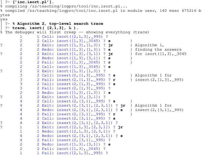
Figure 1: Algorithm 2 (top-level trace) for $isort([2,1,3],L)$

Figure 1 presents constructing a top-level trace for a query $isort([2,1,3],L)$, by Algorithm 2. Margin comments show the fragments of the trace obtained by Algorithm 1 (finding all the answers to a query). The Call and Exit items in these fragments are the top-level trace for the given initial query. So the top-level trace is:

query answers isort([1,3],_3045) isort([1,3],[1,3]) isort([1,3],[3,1]) insert(2,[1,3],_995) (none) insert(2,[3,1],_995) insert(2,[3,1],[2,3,1])

Algorithm 4

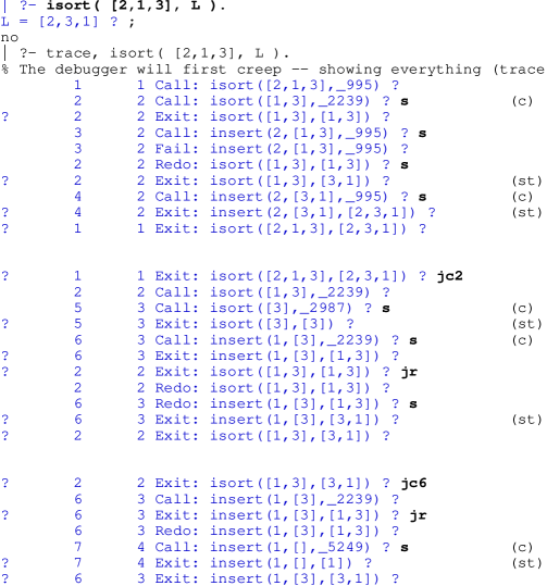
Figure 2: Incorrectness diagnosis according to Algorithm 4

Figure 2 presents diagnosing incorrectness (Algorithm 4) for query $isort([2,1,3],L)$. The debugging output is split into three parts, each is a construction of a top-level success trace (Algorithm 3). The elements of such success trace are marked with (st) in the margin, the corresponding calls are marked with (c).

First the top-level (search) trace is constructed until arriving to the incorrect answer isort([2,1,3],[2,3,1]), we skip invocations of Algorithm 1. Then we pick from the debugger output the top-level success trace for this atom.

The success trace consists of two items (formally - of the atoms of items):

    4      2 Exit: insert(2,[3,1],[2,3,1])
    2      2 Exit: isort([1,3],[3,1])

The latter is incorrect. (Note that, according to the specification for correctness, atom insert(2,[3,1],[2,3,1]) is correct - we do not bother how items are inserted into non sorted lists.)

Now command jc2 leads to the call $isort([1,3],\_2239)$ that corresponds to the incorrect atom. We obtain a relevant fragment of the top-level trace for this call, and search it for the top-level success trace; its items are

    6      3 Exit: insert(1,[3],[3,1])
    5      3 Exit: isort([3],[3]) ?

The former is incorrect, jc6 leads to the corresponding call. The top-level call trace consists of one item

    7      4 Exit: insert(1,[],[1])

(the debugger does not show invocations of built-in predicates =</2, >/2). As the top-level success trace for the incorrect atom $insert(1,[3],[3,1])$ consists only of correct atoms, we located an incorrect clause. It is the last clause of the program (as $insert(1,[3],[3,1])$ is an instance of its head, and - apart from built-ins - it has a single body atom, of which $insert(1,[\,],[1])$ is an instance).

Algorithm 5

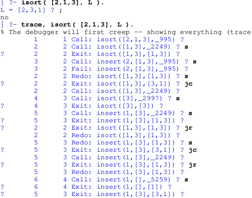
Figure 3: Incorrectness diagnosis according to Algorithm 5

Figure 3 presents applying Algorithm 5 to query $isort([2,1,3],L)$. Whenever an incorrect answer is encountered, command jc is issued to go to the corresponding Call item. So recursive invocations of the algorithm were performed for $isort([1,3],\_2249)$ and $insert(1,[3],\_2249)$. Note that the resulting trace is an abbreviation of that of Algorithm 4. The located incorrect clause is the same as in the previous example.

Figure 4: Incorrectness diagnosis according to Algorithm 5, with the incorrect answer as the initial query.

Figure 4 shows that in this particular case the search of Algorithm 5 is not made shorter by beginning from the incorrect answer to the considered query (instead of beginning from the query itself).

Note that, in the top-level trace for $isort([1,3],\_2249)$, we could not jump over the fragment leading to the first, correct answer. If we do so, the Prolog debugger misses crucial fragments of the computation leading the the second, wrong answer. See Figure 5. After the jc command leading to Call:  isort([1,3],_2239), command s was issued, to immediately obtain the first answer. As a result, $insert(1,[3],\_2249)$ was not traced at all.

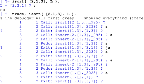
Figure 5: Incorrect application of Algorithm 5, due to jumping over supposedly irrelevant fragments of the top-level trace

Declarative diagnosis of incorrectness

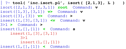
Figure 6: Declarative incorrectness diagnosis of the same error

For a comparison, Figure 6 presents declarative incorrectness diagnosis of the program used above, with the same initial query.

Note that declarative diagnosis is substantially simpler and more efficient than that using the Prolog debugger, exemplified above. In particular, its log is shorter and much simpler to understand.

Some explanations are due. The tool used is a prototype browser for proof trees. It displays the current tree node (an atom) and asks for a command. For non-root nodes it displays (in green) the applicable navigation commands. These commands are:

v   -- go to the child,

<   -- go to the left sibling,

>   -- go to the right sibling,

So we know if the current node is a leaf, a leftmost sibling, or a rightmost one. (A command moving to the parent is not displayed and is not used here.)

Declarative incorrectness diagnosis is performed by navigating the tree looking for an incorrect child of the last found incorrect node. Eventually we arrive at one without incorrect children. In our case such correct children are $3>1$ and $insert(1,[\,],[1])$. This means finding an incorrectness error (an instance of an incorrect clause). Command s displays (in red) the error. (Technically, it displays the parent of the current node with all its children.)

It is important that the user does not face a strict declarative diagnosis algorithm, which only asks questions. Instead, the user decides, what to do. For instance, when correctness of a given atom is not obvious (say the atom is big), one may look at its siblings first. One may explore a subtree, and then move back; etc.

3 Diagnosing incompleteness

Here we use another buggy version of the program, ins.isort.pl (in the names of programs “inc” abbreviates “incorrectness, and “ins” - “insufficiency”, a synonym for incompleteness):

        isort([X|Xs],Ys) :- isort(Xs,Zs), insert(X,Zs,Ys).
        isort([],[]).

        insert(X,[Y|Ys],[Y|Zs]) :- X > Y, insert(X,Ys,Zs).
        insert(X,[Y|Ys],[X,Y|Ys]) :- X =< Y.

No answer is obtained for query $isort([3,2,1],L)$, thus it is an incompleteness symptom.

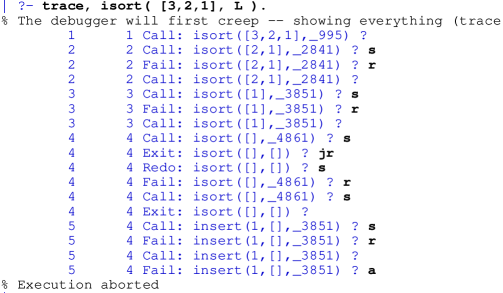
Figure 7: Incompleteness diagnosis according to Algorithm 6.

Algorithm 6

Applying algorithm 6 for query $isort([3,2,1],L)$ is shown in Figure 7. Construction of a top-level trace (Algorithm 2) is begun. The trace contains an incompleteness symptom

     2      2 Call: isort([2,1],_2841)

(it fails with no answers). So the construction of the trace is interrupted, and we begin Algorithm 2 for this query (by commands r and “enter”). Here

     3      3 Call: isort([1],_3851)

(which fails) is a symptom; Algorithm 2 is invoked for this query. The top level trace is:

query answers

isort([],_4861) isort([],[])

insert(1,[],_3851) (none)

and $insert(1,[\,],\_3851)$ is a symptom, it is also the located incompleteness error (as it fails immediately, so its top-level trace is empty, by Algorithm 2). Procedure insert has been found to be the reason of incompleteness.

Declarative diagnosis of incompleteness

For a comparison, we present declarative incompleteness diagnosis for the same program and symptom. We use a prototype diagnoser of [DNTM89] (Figure  8).

We should explain the terminology used by the prototype. An atom $A$ being satisfiable means that ${{\it Sp}^{0}}\models\exists A$, where ${{\it Sp}^{0}}$ is the specification for completeness. (In other words, this means that $A$ has an instance which is in ${{\it Sp}^{0}}$.) Also, “not completely covered” means an incompleteness error [Dra19, Def. 9].

Figure 8: Declarative incompleteness diagnosis of the same error

The tool works similarly to Algorithm 6, by constructing top-level search traces. Such trace is searched for an incorrectness symptom, by querying the user about the elements of the trace. The form of the query is simpler when the trace element consists of an atom with no answers. Such simpler queries are asked first. As a result, in the presented example there was no need to ask a more complicated query.

Note the simplicity and efficiency of declarative diagnosis, in comparison with that using the Prolog debugger.

References

- [DNTM89] W. Drabent, S. Nadjm-Tehrani, and J. Małuszyński. Algorithmic Debugging with Assertions. In H. Abramson and M. H. Rogers, editors, Meta-Programming in Logic Programming, pages 501–522. The MIT Press, 1989.
- [Dra16] W. Drabent. Correctness and completeness of logic programs. ACM Trans. Comput. Log., 17(3):18:1–18:32, 2016.
- [Dra19] W. Drabent. The prolog debugger and declarative programming. CoRR, abs/1906.04765, 2019. http://arxiv.org/abs/1906.04765. To appear in Logic-Based Program Synthesis and Transformation 29th International Symposium, LOPSTR 2019, Porto, Portugal, Revised Selected Papers, Lecture Notes in Computer Science, vol. 12042. Springer.
- [Sha83] E. Shapiro. Algorithmic Program Debugging. The MIT Press, 1983.