Online Sinkhorn: Optimal Transport distances from sample streams

Abstract

Optimal Transport (OT) distances are now routinely used as loss functions in ML tasks. Yet, computing OT distances between arbitrary (i.e. not necessarily discrete) probability distributions remains an open problem. This paper introduces a new online estimator of entropy-regularized OT distances between two such arbitrary distributions. It uses streams of samples from both distributions to iteratively enrich a non-parametric representation of the transportation plan. Compared to the classic Sinkhorn algorithm, our method leverages new samples at each iteration, which enables a consistent estimation of the true regularized OT distance. We provide a theoretical analysis of the convergence of the online Sinkhorn algorithm, showing a nearly-$\mathcal{O}(\frac{1}{n})$ asymptotic sample complexity for the iterate sequence. We validate our method on synthetic 1D to 10D data and on real 3D shape data.

Optimal transport (OT) distances are fundamental in statistical learning, both as a tool for analyzing the convergence of various algorithms [7, 13], and as a data-dependent term for tasks as diverse as supervised learning [18], unsupervised generative modeling [3] or domain adaptation [10]. OT lifts a distance over data points living in a space $\mathcal{X}$ into a distance on the space $\mathcal{P}(\mathcal{X})$ of probability distributions over the space $\mathcal{X}$. This distance has many favorable geometrical properties. In particular it allows one to compare distributions having disjoint supports. Computing OT distances is usually performed by sampling once from the input distributions and solving a discrete linear program (LP), due to [25]. This approach is numerically costly and statistically inefficient [44]. Furthermore, the optimisation problem depends on a fixed sampling of points from the data. It is therefore not adapted to machine learning settings where data is resampled continuously (e.g. in GANs), or accessed in an online manner. In this paper, we develop an efficient online method able to estimate OT distances between continuous distributions. It uses a stream of data to refine an approximate OT solution, adapting the regularized OT approach to an online setting.

To alleviate both the computational and statistical burdens of OT, it is common to regularize the Kantorovich LP. The most successful approach in this direction is to use an entropic barrier penalty. When dealing with discrete distributions, this yields a problem that can be solved numerically using Sinkhorn-Knopp’s matrix balancing algorithm [38, 39]. This approach was pushed forward for ML applications by [11]. Sinkhorn distances are smooth and amenable to GPU computations, which make them suitable as a loss function in model training [18, 30]. The Sinkhorn algorithm operates in two distinct phases: draw samples from the distributions and evaluate a pairwise distance matrix in the first phase; balance this matrix using Sinkhorn-Knopp iterations in the second phase.

This two-step approach does not estimate the true regularized OT distance, and cannot handle samples provided as a stream, e.g. renewed at each training iteration of an outer algorithm. A cheap fix is to use Sinkhorn over mini-batches (see for instance [21] for an application to generative modelling). Yet this introduces a strong estimation bias, especially in high dimension —see [16] for a mathematical analysis. In contrast, we use streams of mini-batches to progressively enrich a consistent representation of the transport plan.

Contributions.

Our paper proposes a new take on estimating optimal transport distances between continuous distributions. We make the following contributions:

• We introduce an online variant of the Sinkhorn algorithm, that relies on streams of samples to enrich a non-parametric functional representation of the dual regularized OT solution.

• We establish the almost sure convergence of online Sinkhorn and derive asymptotic convergence rates (Proposition 3 and 4). We provide convergence results for variants.

• We demonstrate the performance of online Sinkhorn for estimating OT distances between continuous distributions and for accelerating the early phase of discrete Sinkhorn iterations.

Notations.

We denote $\mathcal{C}(\mathcal{X})$ [$\mathcal{C}_{+}(\mathcal{X})$] the set of [strictly positive] continuous functions over a metric space $\mathcal{X}$, $\mathcal{M}^{+}(\mathcal{X})$ and $\mathcal{P}(\mathcal{X})$ the set of positive and probability measures on $\mathcal{X}$, respectively.

1 Related work

Sinkhorn properties.

The Sinkhorn algorithm computes $\varepsilon$-accurate approximations of OT in $O(n^{2}/\varepsilon^{3})$ operations for $n$ samples [2] (in contrast with the $\mathcal{O}(n^{3})$ complexity of exact OT [22]). Moreover, Sinkhorn distances suffer less from the curse of dimensionality [19], since the average error using $n$ samples decays like $\mathcal{O}(\varepsilon^{-d/2}/\sqrt{n})$ in dimension $d$, in contrast with the slow $\mathcal{O}(1/n^{1/d})$ error decay of OT [15, 44]. Sinkhorn distances can further be sharpened by entropic debiasing [17]. Our work is orthogonal, as we focus on estimating distances between continuous distributions.

Continuous optimal transport.

Extending OT computations to arbitrary distributions (possibly having continuous densities) without relying on a fixed a priori sampling is an emerging topic of interest. A special case is the semi-discrete setting, where one of the two distributions is discrete. Without regularization, over an Euclidean space, this can be solved efficiently using the computation of Voronoi-like diagrams [31]. This idea can be extended to entropic-regularized OT [12], and can also be coupled with stochastic optimization methods [20] to tackle high=dimensional problems (see [40] for an extension to Wasserstein barycenters). When dealing with arbitrary continuous densities, that are accessed through a stream of random samples, the challenge is to approximate the (continuous) dual variables of the regularized Kantorovich LP using parametric or non-parametric classes of functions. For application to generative model fitting, one can use deep networks, which leads to an alternative formulation of Generative Adversarial Networks (GANs) [3] (see also [37] for an extension to the estimation of transportation maps). There is however no theoretical guarantees for this type of dual approximations, due to the non-convexity of the resulting optimization problem. To our knowledge, the only mathematically rigorous algorithm represents potentials in reproducing Hilbert space [20]. This approach is generic and does not leverage the specific structure of the OT problem, so that in practice its convergence is slow. We show in Section §5.1 that online Sinkhorn finds better potential estimates than SGD on RKHS representations.

Stochastic approximation (SA).

Our approach may be seen as SA [35] for finding the roots of an operator in a non-Hilbertian functional space. [1] studies SA for solving fixed-points that are contractant in Hilbert spaces. Online Sinkhorn convergence relies on the contractivity of a certain operator in a non-Hilbertian metric, and requires a specific analysis. As both are SA instances, the online Sinkhorn algorithm resembles stochastic EM [8], though it cannot be interpreted as such.

2 Background: optimal transport distances

We first recall the definition of optimal transport distances between arbitrary distributions (i.e. not necessarily discrete), then review how these are estimated using a finite number of samples.

2.1 Optimal transport distances and algorithms

Wasserstein distances.

We consider a complete metric space $(\mathcal{X},d)$ (assumed to be compact for simplicity), equipped with a continuous cost function $(x,y)\in\mathcal{X}^{2}\to C(x,y)\in\mathbb{R}$ for any $(x,y)\in\mathcal{X}^{2}$ (assumed to be symmetric also for simplicity). Optimal transport lifts this ground cost into a cost between probability distributions over the space $\mathcal{X}$. The Wasserstein cost between two probability distributions $(\alpha,\beta)\in\mathcal{P}(\mathcal{X})^{2}$ is defined as the minimal cost required to move each element of mass of $\alpha$ to each element of mass of $\beta$. It rewrites as the solution of a linear problem (LP) over the set of transportation plans (which are probability distribution $\pi$ over $\mathcal{X}\times\mathcal{X}$):

$$\mathcal{W}_{C,0}(\alpha,\beta)\triangleq\min_{\pi\in\mathcal{P}(\mathcal{X}^{2})}\left\{\langle C,\,\pi\rangle\;:\;\pi_{1}=\alpha,\pi_{2}=\beta\right\},$$ (1)

where we denote $\langle C,\,\pi\rangle\triangleq\int C(x,y)\textrm{d}\pi(x,y)$. Here, $\pi_{1}=\int_{y\in\mathcal{X}}\textrm{d}\pi(\cdot,y)$ and $\pi_{2}=\int_{x\in\mathcal{X}}\textrm{d}\pi(x,\cdot)$ are the first and second marginals of the transportation plan $\pi$. We refer to [36] for a review on OT.

Entropic regularization and Sinkhorn algorithm.

The solutions of (2) can be approximated by a strictly convex optimisation problem, where an entropic term is added to the linear objective to force strict convexity. The so-called Sinkhorn cost is then

$$\mathcal{W}_{C,\varepsilon}(\alpha,\beta)\triangleq\min_{\begin{subarray}{c}\pi\in\mathcal{P}(\mathcal{X}\times\mathcal{X})\\ \pi_{1}=\alpha,\pi_{2}=\beta\end{subarray}}\langle C,\,\pi\rangle+\varepsilon\textrm{KL}(\pi|\alpha\otimes\beta),$$ (2)

where the Kulback-Leibler divergence is defined as $\textrm{KL}(\pi|\alpha\otimes\beta)\triangleq\int\log(\frac{\textrm{d}\pi}{\textrm{d}\alpha\textrm{d}\beta})\textrm{d}\pi$ (which is thus equal to the mutual information of $\pi$). $\mathcal{W}_{C,\varepsilon}$ approximates $\mathcal{W}_{C,0}(\alpha,\beta)$ up to an $\varepsilon\log(\varepsilon)$ error [19]. In the following, we set $\varepsilon$ to $1$ without loss of generality, as $\mathcal{W}_{C,\varepsilon}=\varepsilon\mathcal{W}_{C/\varepsilon,1}$, and simply write $\mathcal{W}$. (2) admits a dual form, which is a maximization problem over the space of continuous functions:

$$F_{\alpha,\beta}(f,g)\triangleq\max_{(f,g)\in\mathcal{C}(\mathcal{X})^{2}}\langle f,\,\alpha\rangle+\langle g,\,\beta\rangle-\langle e^{f\oplus g-C},\,\alpha\otimes\beta\rangle+1,$$ (3)

where $\langle f,\,\alpha\rangle\triangleq\int f(x)\textrm{d}\alpha(x)$ and $(f\oplus g-C)(x,y)\triangleq f(x)+g(y)-C(x,y)$. Problem (3) can be solved by closed-form alternated maximization, which corresponds to Sinkhorn’s algorithm. At iteration $t$, the updates are simply

$$f_{t+1}(\cdot) =T_{\beta}(g_{t}),\quad g_{t+1}(\cdot)=T_{\alpha}(f_{t+1}),$$ (4)

$$T_{\mu}(h) \triangleq-\log\int_{y\in\mathcal{X}}\!\!\exp(h(y)-C(\cdot,y))\textrm{d}\mu(y).$$ (5)

The operation $h\mapsto T_{\mu}(h)$ maps a continuous function to another continuous function, and is a smooth approximation of the celebrated $C$-transform of OT [36]. We thus refer to it as a soft C-transform. Note that we consider simultaneous updates of $f_{t}$ and $g_{t}$ in this paper, as it simplifies our analysis. The notation $f_{t}(\cdot)$ emphasizes the fact that $f_{t}$ and $g_{t}$ are functions.

It can be shown that ${(f_{t})}_{t}$ and ${(g_{t})}_{t}$ converge in $(\mathcal{C}(\mathcal{X}),\left\|\cdot\right\|_{\text{var}})$ to a solution $(f^{\star},g^{\star})$ of (3), where $\left\|f\right\|_{\text{var}}\triangleq\max_{x}f(x)-\min_{x}f(x)$ is the so-called variation norm. Functions endowed with this norm are only considered up to an additive constant. Global convergence is due to the strict contraction of the operators $T_{\beta}(\cdot)$ and $T_{\alpha}(\cdot)$ in the space $(\mathcal{C}(\mathcal{X}),\left\|\cdot\right\|_{\text{var}})$ [28].

2.2 Estimating OT distances with realizations

When the input distributions are discrete (or equivalently when $\mathcal{X}$ is a finite set), i.e. $\alpha=\frac{1}{n}\sum_{i=1}^{n}\delta_{x_{i}}$ and $\beta=\frac{1}{n}\sum_{i=1}^{n}\delta_{y_{i}}$, the function $f_{t}$ and $g_{t}$ need only to be evaluated on $(x_{i})_{t}$ and $(y_{i})_{i}$, which allows a proper implementation. The iterations (5) then correspond to the [39] algorithm over the inverse scaling vectors $\bm{u}_{t}\triangleq{(e^{-f_{t}(x_{i})})}_{i=1}^{n},\bm{v}_{t}\triangleq{(e^{-g_{t}(y_{i})})}_{i=1}^{n}$:

$$\bm{u}_{t+1}=\bm{K}\frac{1}{n\bm{v}_{t}}\quad\text{and}\quad\bm{v}_{t+1}=\bm{K}^{\top}\frac{1}{n\bm{u}_{t}}$$ (6)

where $\bm{K}=(e^{-C(x_{i},y_{i})})_{i,j=1}^{n}\in\mathbb{R}^{n\times n}$, and inversion is made pointwise. The Sinkhorn algorithm for OT thus operates in two phases: first, the kernel matrix $\bm{K}$ is computed, with a cost in $O(n^{2}d)$, where $d$ is the dimension of $\mathcal{X}$; then each iteration (6) costs $O(n^{2})$. The online Sinkhorn algorithm that we propose mixes these two phases to accelerate convergence (see results in §5.2).

Consistency and bias.

The OT distance $\mathcal{W}_{C,0}(\alpha,\beta)$ and its regularized version $\mathcal{W}_{C,\varepsilon}(\alpha,\beta)$ can be approximated by the (computable) distance between discrete realizations $\hat{\alpha}=\frac{1}{n}\sum_{i}\delta_{x_{i}}$, $\hat{\beta}=\frac{1}{n}\sum_{i}\delta_{y_{i}}$, where ${(x_{i})}_{i}$ and ${(y_{i})}_{i}$ are i.i.d samples from $\alpha$ and $\beta$. Consistency holds, as $\mathcal{W}(\hat{\alpha}_{n},\hat{\beta}_{n})\to\mathcal{W}(\alpha,\beta)$. Although this is a reassuring result, the sample complexity of transport in high dimensions with low regularization remains high (see §1).

The estimation of $\mathcal{W}(\alpha,\beta)$ may be improved using several i.i.d sets of samples $(\hat{\alpha}_{t})_{t}$ and ${(\hat{\beta}_{t})}_{t}$. Those should be of reasonable size to fit in memory and may for example come from a temporal stream. [21] use a Monte-Carlo estimate $\hat{\mathcal{W}}(\alpha,\beta)=\frac{1}{T}\sum_{t=1}^{T}\mathcal{W}(\hat{\alpha}_{t},\hat{\beta}_{t})$. However, this yields a biased estimation as the distance $\mathcal{W}(\alpha,\beta)$ and the optimal potentials $f^{\star}=f^{\star}(\alpha,\beta)$ differ from their expectation under sampling $\mathbb{E}_{\hat{\alpha}\sim\alpha,\hat{\beta}\sim\beta}[\mathcal{W}(\hat{\alpha},\hat{\beta})]$ and $\mathbb{E}_{\hat{\alpha}\sim\alpha,\hat{\beta}\sim\beta}[f^{\star}(\hat{\alpha},\hat{\beta})]$. In contrast, online Sinkhorn consistently estimates the true potential functions (up to a constant) and the Sinkhorn cost.

3 OT distances from sample streams

We now introduce an online adaptation of the Sinkhorn algorithm. We construct functional estimators of $f^{\star}$, $g^{\star}$ and $\mathcal{W}(\alpha,\beta)$ using successive discrete distributions of samples ${(\hat{\alpha}_{t})}_{t}$ and ${(\hat{\beta}_{t})}_{t}$, where $\hat{\alpha}_{t}\triangleq\frac{1}{n}\sum_{i=n_{t}+1}^{n_{t+1}}\delta_{x_{i}}$, with $n_{0}\triangleq 0$ and $n_{t+1}\triangleq n_{t}+n$. The size of the mini-batch $n$ may potentially depends on $t$. ${(\hat{\alpha}_{t})}_{t}$ and ${(\hat{\beta}_{t})}_{t}$ may be seen as mini-batches of size $n$ within a training procedure.

3.1 Online Sinkhorn iterations

The optimization trajectory ${(f_{t},g_{t})}_{t}$ of the continuous Sinkhorn algorithm given by (5) is untractable as it cannot be represented in memory. The exp-potentials $u_{t}\triangleq\exp(-f_{t})$ and $v_{t}\triangleq\exp(-g_{t})$ are indeed infinitesimal mixtures of kernel functions $\kappa_{y}(\cdot)\triangleq\exp(-C(\cdot,y))$ and $\kappa_{x}(\cdot)\triangleq\exp(-C(x,\cdot))$.

We propose to construct finite-memory consistent estimates of $u_{t}$ and $v_{t}$ using principles from stochastic approximation (SA) [35]. We cast the regularized OT problem as a root-finding problem of a function-valued operator $\mathcal{F}:\mathcal{C}_{+}(\mathcal{X})\times\mathcal{C}_{+}(\mathcal{X})\to\mathcal{C}(\mathcal{X})\times\mathcal{C}(\mathcal{X})$, for which we can obtained unbiased estimates. Optimal potentials are indeed exactly the roots of

$$\mathcal{F}:(u,v)\to\Big{(}u(\cdot)-\int_{y\in\mathcal{X}}\frac{1}{v(y)}\kappa_{y}(\cdot)\textrm{d}\beta(y),\quad v(\cdot)-\int_{x\in\mathcal{X}}\frac{1}{u(x)}\kappa_{x}(\cdot)\textrm{d}\alpha(x)\Big{)}.$$ (7)

In particular, the simultaneous Sinkhorn updates rewrites as $(u_{t+1},v_{t+1})=(u_{t},v_{t})-\mathcal{F}(u_{t},v_{t})$ for all $t$. Importantly, $\mathcal{F}$ can be evaluated without bias using two empirical measures $\hat{\alpha}$ and $\hat{\beta}$, defining

$$\hat{\mathcal{F}}_{\hat{\alpha},\hat{\beta}}(u,v)\triangleq\Big{(}u(\cdot)-\frac{1}{n}\sum_{i=1}^{n}\frac{1}{v(y_{i})}\kappa_{y_{i}}(\cdot)\quad v(\cdot)-\frac{1}{n}\sum_{i=1}^{n}\frac{1}{u(x_{i})}\kappa_{x_{i}}(\cdot)\Big{)}.$$ (8)

By construction, $\mathbb{E}_{\hat{\alpha}\sim\alpha,\hat{\beta}\sim\beta}[\hat{\mathcal{F}}_{\hat{\alpha},\hat{\beta}}]=\mathcal{F}$, and the images of $\hat{\mathcal{F}}$ admit a representation in memory.

Randomized Sinkhorn.

To make use of a stream of samples $(\hat{\alpha}_{t},\hat{\beta}_{t})_{t}$, we may simply replace $\mathcal{F}$ with $\hat{\mathcal{F}}$ in the Sinkhorn updates. This amounts to use noisy soft $C$-transforms in (5), as we set

$$(u_{t+1},v_{t+1}) \triangleq(u_{t},v_{t})-\hat{\mathcal{F}}_{\hat{\alpha},\hat{\beta}}(u_{t},v_{t}),\quad\text{i.e.}$$ (9)

$$\hat{f}_{t+1} =T_{\hat{\beta}_{t}}(\hat{g}_{t}),\qquad\hat{g}_{t+1}=T_{\hat{\alpha}_{t}}(\hat{f}_{t+1}).$$ (10)

$\hat{f}_{t}$ and $\hat{g}_{t}$ are defined in memory by $(y_{i},\hat{g}_{t-1}(y_{i}))_{i}$ and $(x_{i},\hat{f}_{t-1}(x_{i}))_{i}$. Yet the variance of the updates (9) does not decay through time, hence this randomized Sinkhorn algorithm does not converge. However, we show in Proposition 1 that the Markov chain ${(\hat{f}_{t},\hat{g}_{t})}_{t}$ converges towards a stationary distribution that is independent of the potentials $\hat{f}_{0}$ and $\hat{g}_{0}$ used for initialization.

Online Sinkhorn.

To ensure convergence of $\hat{f}_{t}$, $\hat{g}_{t}$ towards some optimal pair of potentials $(f^{\star},g^{\star})$, one must take more cautious steps, in particular past iterates should not be discarded. We introduce a learning rate $\eta_{t}$ in Sinkhorn iterations, akin to the Robbins-Monro algorithm for finding roots of vector-valued functions:

$$(\hat{u}_{t+1},\hat{v}_{t+1}) \triangleq(1-\eta_{t})(\hat{u}_{t},\hat{v}_{t})-\eta_{t}\hat{\mathcal{F}}_{\hat{\alpha}_{t},\hat{\beta}_{t}}(\hat{u}_{t},\hat{v}_{t}),\quad\text{i.e.}$$ (11)

$$e^{-\hat{f}_{t+1}} =(1-\eta_{t})e^{-\hat{f}_{t}}+\eta_{t}e^{-T_{\hat{\beta}_{t}}(\hat{g}_{t})}$$ (12)

Each update adds new kernel functions to a non-parametric estimation of $u_{t}$ and $v_{t}$. The estimates $\hat{u}_{t}$ and $\hat{v}_{t}$ are defined by weights ${(p_{i,t},q_{i,t})}_{i\leqslant n_{t}}$ and positions ${(x_{i},y_{i})}_{i\leqslant n_{t}}\subseteq\leavevmode\nobreak\ \mathcal{X}^{2}$:

$$e^{-\hat{f}_{t}(\cdot)} =\hat{u}_{t}(\cdot)\triangleq\sum_{i=1}^{n_{t}}\exp(q_{i,t}-C(\cdot,y_{i})),$$ (13)

$$e^{-\hat{g}_{t}(\cdot)} =\hat{v}_{t}(\cdot)\triangleq\sum_{i=1}^{n_{t}}\exp(p_{i,t}-C(x_{i},\cdot)).$$ (14)

The SA updates (11) yields simple vectorized updates for the weights ${(p_{i},q_{i})}_{i}$, leading to Algorithm 1. We perform the updates for $q_{i}$ and $p_{i}$ in log-space, for numerical stability reasons.

Complexity.

Each iteration of online Sinkhorn has complexity $\mathcal{O}(n_{t}\,n)$, due to the evaluation of the distances $C(x_{i},y_{i})$ for all $(x_{i})_{(0,n_{t}]}$ and $(y_{i})_{(n_{t},n_{t+1}]}$, and the soft $C$-transforms in (13). Online Sinkhorn computes a distance matrix $(C(x_{i},y_{j}))_{i,j\leqslant n_{t}}$ on the fly, in parallel to updating $\hat{f}_{t}$ and $\hat{g}_{t}$. In total, its computation cost after drawing $n_{t}$ samples is $\mathcal{O}(n_{t}^{2})$. Its memory cost is $\mathcal{O}(n_{t})$; it increases with iterations, which is a requirement for consistent estimation. Randomized Sinkhorn with constant batch-sizes $n$ has a memory cost of $\mathcal{O}(n)$ and a single-iteration computational cost of $\mathcal{O}(n^{2})$.

Input: Dist. $\alpha$ and $\beta$, learning weights ${(\eta_{t})}_{t}$, batch sizes ${(n(t))}_{t}$ Set $p_{i}=q_{i}=0$ for $i\in(0,n_{1}]$

for $t=0,\dots,{T-1}$ do

     Sample $(x_{i})_{(n_{t},n_{t+1}]}\sim\alpha$, $(y_{j})_{(n_{t},n_{t+1}]}\sim\beta$.

     Evaluate $(\hat{f}_{t}(x_{i}))_{i=(n_{t},n_{t+1}]}$, $(\hat{g}_{t}(y_{i}))_{i=(n_{t},n_{t+1}]}$ using $(q_{i,t},p_{i,t},x_{i},y_{i})_{i=(0,n_{t}]}$ in (13).

     $q_{(n_{t},n_{t+1}],t+1}{\leftarrow}\log\frac{\eta_{t}}{n}+(\hat{g}_{t}(y_{i}))_{(n_{t},n_{t+1}]}$,   $p_{(n_{t},n_{t+1}],t+1}{\leftarrow}\log\frac{\eta_{t}}{n}+(\hat{f}_{t}(x_{i}))_{(n_{t},n_{t+1}]}$.

     $q_{(0,n_{t}],t+1}\leftarrow q_{(0,n_{t}],t}+\log(1-\eta_{t})$,   $p_{(0,n_{t}],t+1}\leftarrow p_{(0,n_{t}],t}+\log(1-\eta_{t})$.

Returns: $\hat{f}_{T}:(q_{i,T},y_{i})_{(0,n_{T}]}$ and $\hat{g}_{T}:(p_{i,T},x_{i})_{(0,n_{T}]}$

Algorithm 1 Online Sinkhorn

3.2 Refinements

Estimating Sinkhorn distance.

As we will see in §4, the iterations (11) only estimate potential functions up to a constant. This is sufficient for minimizing a loss function involving a Sinkhorn distance (e.g. for model training or barycenter estimation [40]), as backpropagating through the Sinkhorn distance relies only on the gradients of the potentials $\nabla_{x}f^{\star}(\cdot)$, $\nabla_{y}g^{\star}(\cdot)$ [12, e.g.]. With extra $\mathcal{O}(n_{t}^{2})$ operations, $(\hat{f}_{t},\hat{g}_{t})$ may be used to estimate $\mathcal{W}(\alpha,\beta)$ through a final soft $C$-transform:

$$\hat{\mathcal{W}}_{t}\triangleq\frac{1}{2}\Big{(}\langle\bar{\alpha}_{t},\,f_{t}+T_{\bar{\alpha}_{t}}(\hat{g}_{t})\rangle{+}\langle\bar{\beta}_{t},\,\hat{g}_{t}{+}T_{\bar{\alpha}_{t}}(f_{t})\rangle\Big{)},$$ (15)

where $\bar{\alpha}_{t}\triangleq\frac{1}{n_{t}}\sum_{i=1}^{n_{t}}\delta_{x_{i}}$ and $\bar{\beta}_{t}$ are formed of all previously observed samples.

Fully-corrective scheme.

The potentials $\hat{f}_{t}$ and $\hat{g}_{t}$ may be improved by refitting the weights $(p_{i})_{(0,n_{t}]}$, $(q_{j})_{(0,n_{t}]}$ based on all previously seen samples. For this, we update $\hat{f}_{t+1}=T_{\bar{\beta}_{t}}(g_{t})$ and $\hat{g}_{t+1}=T_{\bar{\alpha}_{t}}(f_{t})$. This reweighted scheme (akin to the fully-corrective Frank-Wolfe scheme from [26]) has a cost of $\mathcal{O}(n_{t}^{2})$ per iteration. It requires to keep in memory (or recompute on-the-fly) the whole distance matrix. Fully-corrective online Sinhorn enjoys similar convergence properties as regular online Sinkhorn, and permits the use of non-increasing batch-sizes—see §B.1. In practice, it can be used every $k$ iterations, with $k$ increasing with $t$. Combining partial and full updates can accelerate the estimation of Sinkhorn distances (see §5.2).

Finite samples.

Finally, we note that our algorithm can handle both continuous or discrete distributions. When $\alpha$ and $\beta$ are discrete distributions of size $N$, we can store $p$ and $q$ as fixed-size vectors of size $N$, and update at each iterations a set of coordinates of size $n<N$. The resulting algorithm is a subsampled Sinkhorn algorithm for histograms, which is detailed in §B.2, Algorithm 3. We show in §5 that it is useful to accelerate the first phase of the Sinkhorn algorithm.

4 Convergence analysis

We show a stationary distribution convergence property for the randomized Sinkhorn algorithm, an approximate convergence property for the online Sinkhorn algorithm with fixed batch-size and an exact convergence result for online Sinkhorn with increasing batch sizes, with asymptotic convergence rates. We make the following classical assumption on the cost regularity and compactness of $\alpha$ and $\beta$.

Assumption 1.

The cost $C:\mathcal{X}\times\mathcal{X}\to\mathbb{R}$ is $L$-Lipschitz, and $\mathcal{X}$ is compact.

4.1 Randomized Sinkhorn

We first state a result concerning the randomized Sinkhorn algorithm (9), proved in §A.2.

Proposition 1.

Under Assumption 1, the randomized Sinkhorn algorithm (9) yields a time-homogeneous Markov chain ${(\hat{f}_{t},\hat{g}_{t})}_{t}$ which is $(\hat{\alpha}_{s},\hat{\beta}_{s})_{s\leqslant t}$ measurable, and converges in law towards a stationary distribution $(f_{\infty},g_{\infty})\in\mathcal{P}(\mathcal{C}(\mathcal{X})^{2})$ independent of the initialization point $(f_{0},g_{0})$.

This result follows from [14] convergence theorem on iterated random functions which are contracting on average. We use the fact that $T_{\hat{\beta}}(\cdot)$ and $T_{\hat{\alpha}}(\cdot)$ are uniformly contracting, independently of the distributions $\hat{\alpha}$ and $\hat{\beta}$, for the variational norm $\|\cdot\|_{\text{var}}$. Using the law of large number for Markov chains [6], the (tractable) average $\frac{1}{t}\sum_{s=1}^{t}\exp(-\bar{f}_{s})$ converges almost surely to $\mathbb{E}[e^{-f_{\infty}}]\in\mathcal{C}(\mathcal{X})$. This expectation verifies the functional equations

$$\mathbb{E}[e^{-f_{\infty}}]=\int_{y}\mathbb{E}[e^{g_{\infty}(y)-C(\cdot,y)}]\textrm{d}\beta(y)\quad\mathbb{E}[e^{-g_{\infty}}]=\int_{x}\mathbb{E}[e^{f_{\infty}(x)-C(x,\cdot)}]\textrm{d}\alpha(x)$$ (16)

These equations are close to the Sinkhorn fixed point equations, and get closer as $\varepsilon$ increases, since $\varepsilon\mathbb{E}[\exp(\pm f_{\infty}/\varepsilon)]\to\mathbb{E}[\pm f_{\infty}]$ as $\varepsilon\to\infty$. Running the random Sinkhorn algorithm with averaging fails to provide exactly the dual solution, but solves an approximate problem.

4.2 Online Sinkhorn

We make the following [35] assumption on the weight sequence. We then state an approximate convergence result for the online Sinkhorn algorithm with fixed batch-size $n(t)=n$.

Assumption 2.

${(\eta_{t})}_{t}$ is such that $\sum\eta_{t}=\infty$ and $\sum\eta_{t}^{2}<\infty$, $0\leqslant\eta_{t}\leqslant 1$ for all $t>0$.

Proposition 2.

Under Assumption 1 and 2, the online Sinkhorn algorithm (Algorithm 1) yields a sequence $(f_{t},g_{t})$ that reaches a ball centered around $f^{\star},g^{\star}$ for the variational norm $\|\cdot\|_{\text{var}}$. Namely, there exists $T>0$, $A>0$ such that for all $t>T$, almost surely

$$\|f_{t}-f^{\star}\|_{\text{var}}+\|g_{t}-g^{\star}\|_{\text{var}}\leqslant\frac{A}{\sqrt{n}}.$$ (17)

The proof is reported in §A.3. It is not possible to ensure the convergence of online Sinkhorn with constant batch-size. This is a fundamental difference with other SA algorithms, e.g. SGD on strongly convex objectives (see [33]). This stems from the fact that the metric for which $\text{Id}-\mathcal{F}$ is contracting is not a Hilbert norm. The constant $A$ depends on $L$, the diameter of $\mathcal{X}$ and the regularity of potentials $f^{\star}$ and $g^{\star}$, but not on the dimension. It behaves like $\exp(\frac{1}{\varepsilon})$ when $\varepsilon\to 0$. Fortunately, we can show the almost sure convergence of the online Sinkhorn algorithm with slightly increasing batch-size $n(t)$ (that may grow arbitrarily slowly for $\eta_{t}=\frac{1}{t}$), as specified in the following assumption.

Assumption 3.

For all $t>0$, $n(t)=\frac{B}{w_{t}^{2}}\in\mathbb{N}$ and $0\leqslant\eta_{t}\leqslant 1$. $\sum w_{t}\eta_{t}<\infty$ and $\sum\eta_{t}=\infty$.

Proposition 3.

Under Assumption 1 and 3, the online Sinkhorn algorithm converges almost surely:

$$\|\hat{f}_{t}-f^{\star}\|_{\text{var}}+\|\hat{g}_{t}-g^{\star}\|_{\text{var}}\to 0.$$ (18)

The proof is reported in §A.4. It relies on a uniform law of large number for functions [42] and on the uniform contractivity of soft $C$-transform operator [43, e.g.]. Consistency of the iterates is an original property—[20] only show convergence of the OT value. Finally, using bounds from [33], we derive asymptotic rates of convergence for online Sinkhorn (see §A.5), with respect to the number of observed samples $N$. We write $\delta_{N}=\|\hat{f}_{t(N)}-f^{\star}\|_{\text{var}}+\|\hat{g}_{t(N)}-g^{\star}\|_{\text{var}}$, where $t(N)$ is the iteration number for which $n_{t}>N$ samples have been observed.

Proposition 4.

For all $\iota\in(0,1)$, $S>0$ and $B\in\mathbb{N}^{\star}$, setting $\eta_{t}=\frac{S}{t^{1-\iota}}$, $n(t)=\lceil Bt^{4\iota}\rceil$, there exists $D>0$ independant of $N$ and $N_{0}>0$ such that, for all $N>N_{0}$, $\delta_{N}\leqslant\frac{D}{N^{\frac{1-\iota}{1+4\iota}}}$.

Online Sinkhorn thus provides estimators of potentials whose asymptotic sample complexity in variational norm is arbitrarily close to $\mathcal{O}(\frac{1}{N})$. To the best of our knowledge, this is an original property. It also results in a distance estimator $\hat{\mathcal{W}}_{N}$ whose complexity is arbitrarily close to $\mathcal{O}(\frac{1}{\sqrt{N}})$, recovering existing asymptotic rates from [19], for any Lipschitz cost. We derive non-asymptotic rates in §A.5 (see (71)), which make explicit the bias-variance trade-off when choosing the step-sizes and batch-sizes. We also give the explicit form of $D$; it does not depend on the dimension. For low $\varepsilon$, $D$ is proportional to $\exp(\frac{2}{\varepsilon})$; the bound is therefore vacuous for $\varepsilon\to 0$. Note that using growing batch-sizes amounts to increase the budget of a single iteration over time: the overall computational complexity after seeing $N$ samples is always $\mathcal{O}(N^{2})$.

Batch-sizes and step-sizes.

To provide practical guidance on choosing rates in batch-sizes $n(t)$ and step-sizes $\eta_{t}$, we can parametrize $\eta_{t}=\frac{1}{t^{a}}$ and $n(t)=Bt^{b}$ and study what is implied by Assumption 3 and Assumption 4. We summarize the schedules for which convergence is guarantees in Table 1. Note that in practice, it is useful to replace $t$ by $(1+r\,t)$ in these schedules. We set $r=0.1$ in all experiments.

Table 1: Schedules of batch-sizes and learning rates that ensures online Sinkhorn convergence.

Param. schedule	Online Sinkhorn	Fully-corrective online Sinkhorn
Batch size $\displaystyle n(t)=Bt^{b}$	$0<b$	$0\leqslant b$
Step size $\displaystyle\eta_{t}=\frac{1}{t^{a}}$	$\displaystyle a\geqslant 1-\frac{b}{2}$	$$\left\{\begin{aligned} a&>\frac{1}{2}-\frac{b}{2}\quad\text{and}\quad b<1\\ a&\geqslant 0\quad\text{and}\quad b\geqslant 1\end{aligned}\right.$$ (19)

Mirror descent interpretation.

Online Sinkhorn can be interpreted as a non-convex stochastic mirror-descent, as detailed in Appendix D. It provides an original interpretation of the Sinkhorn algorithm, different from recent work [27, 32].

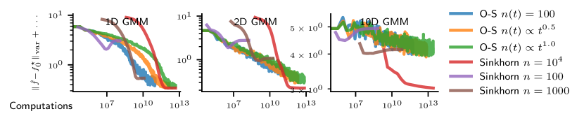
Figure 1: Online Sinkhorn consistently estimate the true regularized OT potentials. Convergence here is measured in term of distance with potentials evaluated on a "test" grid of size $n=10^{4}$. Online-Sinkhorn can estimate potentials faster than sampling then scaling the cost matrix.

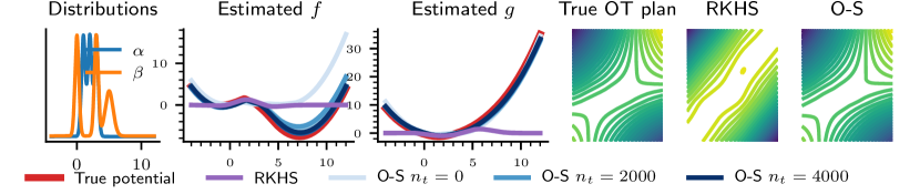
Figure 2: Online Sinhkorn finds the correct potentials over all space, unlike SGD over a RKHS parametrization of the potentials. The plan is therefore correctly estimated everywhere.

5 Numerical experiments

The major purpose of online Sinkhorn (OS) is to handle OT between continuous distributions. We first show that it is a valid alternative to applying Sinkhorn on a single realization of continuous distributions, using examples of Gaussian mixtures of varying dimensions. We then illustrate that OS is able to estimate precisely Kantorovich dual potentials, significantly improving the result obtained using SGD with RKHS expansions [20]. Finally, we show that OS is an efficient warmup strategy to accelerate Sinkhorn for discrete problems on several real and synthetic datasets.

5.1 Continuous potential estimation with online Sinkhorn

Data and quantitative evaluation.

We measure the performance of our algorithm in a continuous setting, where $\alpha$ and $\beta$ are parametric distributions (Gaussian mixtures in 1D, 2D and 10D, with 3, 3 and 5 modes, so that $C_{\max}\sim 1$), from which we draw samples. In the absence of reference potentials $(f^{\star},g^{\star})$ (which cannot be computed in closed form), we compute “test” potentials $(f^{\star}_{0},g^{\star}_{0})$ on realizations $\hat{\alpha}_{0}$ and $\hat{\beta}_{0}$ of size $10000$, using Sinkhorn. We then compare OS to Sinkhorn runs of various size , trained on realizations $N=(100,1000,10000)$ independent of the reference grid (to avoid reducing the problem to a discrete problem between $\hat{\alpha}_{0}$ and $\hat{\beta}_{0}$). To measure convergence, we compute $\delta_{t}=\|\hat{f}_{t}-f^{\star}_{0}\|_{\text{var}}+\|\hat{g}_{t}-g_{0}^{\star}\|_{\text{var}}$, evaluated on the grid defined by $\hat{\alpha}_{0}$ and $\hat{\beta}_{0}$, which constitutes a Monte-Carlo approximation of the error. We evaluate OS with and without full-correction, with different batch-size schedules (see §C.1), as well as the randomized Sinkhorn algorithm. Quantitative results are average over 5 runs. We report quantitative results for $\varepsilon=10^{-2}$ and non fully-corrective online Sinkhorn in the main text, and all other curves in Supp. Fig. 4. In Supp. Fig. 7, we also report results for OT between Gaussians, which is a simpler and less realistic setup, but for which closed-form expressions of the potentials are known [24].

Comparison to SGD.

For qualitative illustration, on the 1D and 2D problem, we consider the main existing competing approach [20], in which $f_{t}(\cdot)$ is parametrized as $\sum_{i=1}^{n_{t}}\alpha_{t}\kappa(\cdot,x_{i})$ (and similarly for $g_{t}$), where $\kappa$ is a reproducing kernel (typically a Gaussian). This differs significantly from online Sinkhorn, where we express $e^{-f_{t}}$ as a Gaussian mixture. The dual problem (5) is solved using SGD, with convergence guarantees on the dual energy. As advocated by the authors, we run a grid search over the bandwidth parameter $\sigma$ of the Gaussian kernel to select the best performing runs.

Earlier potential convergence.

We study convergence curves in Fig. 1, comparing algorithms at equal number of multiplications. OS outperforms or matches Sinkhorn for $N=100$ and $N=1000$ on the three problems; it approximately matches the performance of Sinkhorn on $N=10000$ new iterates on the 1D and 2D problems. On the two low-dimensional problems, online Sinkhorn converges faster than Sinkhorn at the beginning. Indeed, it initiates the computation of the potentials early, while the Sinkhorn algorithm must wait for the cost matrix to be filled. This leads us to study online Sinkhorn as a catalyser of Sinkhorn in the next paragraph. OS convergence is slower (but is still noticeable) for the higher dimensional problem. Fully-corrective OS performs better in this case (see Supp. Fig. 5). We also note that randomized Sinkhorn with batch-size $N$ performs on par with Sinkhorn of size $N$ (Supp. Fig. 6).

Better-extrapolated potentials.

As illustrated in Fig. 2, in 1D, online Sinkhorn refines the potentials $(\hat{f}_{t},\hat{g}_{t})_{t}$ until convergence toward $(f^{\star},g^{\star})$. Supp. Fig. 8 shows a visualisation for 2D GMM. As the parametrization (13) is adapted to the dual problem, the algorithm quickly identifies the correct shape of the optimal potentials—as predicted by Proposition 3. In particular, OS estimates potentials with much less errors than SGD in a RKHS in areas where the mass of $\alpha$ and $\beta$ is low. This allows to consistently estimate the transport plan, which cannot be achieved using SGD. SGD did not converge for $\varepsilon<10^{-1}$, while online Sinkhorn remains stable. OS does not require to set a bandwidth.

$-\log\varepsilon$	4	3	2	1
Stanford	5.3x	4.4x	2.3x	1.2x
10D GMM	1.4x	1.5x	1.3x	1.2x
2D GMM	17x	3.7x	1.3x	2.0x

Figure 3: Online Sinkhorn allows to warmup Sinkhorn during the evaluation of the cost matrix, and to speed discrete optimal transport. Table 2: Speed-ups provided by OS vs S to reach a $10^{-3}$ precision.

5.2 Accelerating Sinkhorn with online Sinkhorn warmup

The discrete Sinkhorn algorithm requires to compute the full cost matrix $\bm{C}\triangleq(C(x_{i},y_{i}))_{i,j}$ of size $N\times N$, prior to estimating the potentials $\bm{f}_{1}\in\mathbb{R}^{N}$ and $\bm{g}_{1}\in\mathbb{R}^{N}$ by a first $C$-transform. In contrast, online Sinkhorn can progressively compute this matrix while computing first sketches of the potentials. The extra cost of estimating the initial potentials without full-correction is simply $2N^{2}$, i.e. similar to filling-up $\bm{C}$. We therefore assess the performance of online Sinkhorn as Sinkhorn warmup in a discrete setting. Online Sinkhorn is run with batch-size $n$ during the first iterations, until observing each sample of $[1,N]$, i.e. until the cost matrix $\bm{C}$ is completely evaluated. From then, the subsequent potentials are obtained using full Sinkhorn updates. We consider the GMMs of §5.1, as well as a 3D dragon from Stanford 3D scans [41] and a sphere of size $N=12000$. We measure convergence using the error $\|T_{\alpha}(\hat{f}_{t})-\hat{g}_{t}\|_{\text{var}}+\|T_{\beta}(\hat{g}_{t})-\hat{f}_{t}\|_{\text{var}}$, evaluated on the support of $\alpha$ and $\beta$; this error goes to $0$. We use $n(t)=\frac{N}{100}(1+0.1t)^{1/2}$—results vary little with the exponent.

Results.

We report convergence curves for $\varepsilon=10^{-3}$ in Fig. 3, and speed-ups due to OS in Table 1. Convergence curves for different $\varepsilon$ are reported in Supp. Fig. 9. The proposed scheme provides an improvement upon the standard Sinkhorn algorithm. After $N^{2}d$ computations (the cost of estimating the full matrix $C$), both the function value and distance to optimum are lower using OS: the full Sinkhorn updates then relay the online updates, using an accurate initialization of the potentials. The OS warmed-up Sinkhorn algorithm then maintains its advantage over the standard Sinkhorn algorithm during the remaining iterations. The speed gain increases as $\varepsilon$ reduces and the OT problem becomes more challenging. Sampling without replacement brings an additional speed-up.

6 Conclusion

We have extended the classical Sinkhorn algorithm to cope with streaming samples. The resulting online algorithm computes a non-parametric expansion of the inverse scaling variables using kernel functions. In contrast with previous attempts to compute OT between continuous densities, these kernel expansions fit perfectly the structure of the entropic regularization, which is key to the practical efficiently. We have drawn links between regularized OT and stochastic approximation. This opens promising avenues to study convergence rates of continuous variants of Sinkhorn’s iterations. Future work will refine the complexity constants and design adaptive non-parametric potential estimations.

7 Acknowledgements

This work was supported by the European Research Council (ERC project NORIA). A.M thanks Anna Korba for helpful discussions on mirror descent algorithms, and Thibault Séjourné for proof-reading and relevant references.

Appendix A Proofs

We first introduce two useful known lemmas, and prove the propositions in their order of appearance.

A.1 Useful lemmas

First, under Assumption 1, we note that the soft $C$-transforms are uniformly contracting on the distribution space $\mathcal{P}(\mathcal{X})$. This is clarified in the following lemma, extracted from [43], Proposition 19. We refer the reader to the original references for proofs.

Lemma 1.

Unser Assumption 1, let $\kappa=1-\exp(-L\textnormal{diam}(\mathcal{X}))$. For all $\hat{\alpha}\in\mathcal{P}(\mathcal{X})$ and $\hat{\beta}\in\mathcal{P}(\mathcal{X})$, for all $f,f^{\prime},g,g^{\prime}\in\mathcal{C}(\mathcal{X})$,

$${\|T_{\hat{\alpha}}(f^{\prime})-T_{\hat{\alpha}}(f^{\prime})\|}_{\text{var}}\leqslant\kappa{\|f-f^{\prime}\|}_{\text{var}},\quad{\|T_{\hat{\beta}}(g)-T_{\hat{\beta}}(g^{\prime})\|}_{\text{var}}\leqslant\kappa{\|g-g^{\prime}\|}_{\text{var}}.$$ (20)

We will also need a uniform law of large numbers for functions. The following lemma is a consequence of Example 19.7 and Lemma 19.36 of [42], and is copied in Lemma B.6 in [29].

Lemma 2.

Under Assumption 1, let $(f_{t})_{t}$ be an i.i.d sequence in $\mathcal{C}(\mathcal{X})$, such that $\mathbb{E}[f_{0}]=f\in\mathcal{C}(\mathcal{X})$. Then there exists $A>0$ such that, for all $n>0$,

$$\mathbb{E}\sup_{x\in\mathcal{X}}|\frac{1}{n}\sum_{i=1}^{n}f_{i}(x)-f(x)|\leqslant\frac{A}{\sqrt{n}}.$$ (21)

Finally, we need a result on running averages using the sequence ${(\eta_{t})}_{t}$. The following result stems from a simple Abel transform of the law of large number, and is established by [29], Lemma B.7.

Lemma 3.

Let $(\eta_{t})_{t}$ be a sequence of weights meeting Assumption 2. Let $(X_{t})_{t}$ be an i.i.d sequence of real-valued random variables with existing first moment $\mathbb{E}[X_{0}]$. We consider the sequence ${(\bar{X}_{t})}_{t}$ defined by $\bar{X}_{0}\triangleq X_{0}$ and

$$\bar{X}_{t}\triangleq(1-\eta_{t})\bar{X}_{t-1}+\eta_{t}X_{t}.$$ (22)

Then $\bar{X}_{t}\to_{t\to\infty}\mathbb{E}[X_{0}]$.

A.2 Proof of Proposition 1

Proof.

We use Theorem 1 from [14]. For this, we simply note that the space $\mathcal{C}(\mathcal{X})\times\mathcal{C}(\mathcal{X})$ in which the chain ${x_{t}\triangleq(f_{t},g_{t})}_{t}$, endowed with the metric $\rho((f_{1},g_{1}),(f_{2},g_{2}))=\|f_{1}-f_{2}\|_{\text{var}}+\|g_{1}-g_{2}\|_{\text{var}}$, is complete and separable (the countable set of polynomial functions are dense in this space, for example). We consider the operator $A_{\theta}\triangleq T_{\hat{\beta}}(T_{\hat{\alpha}}(\cdot))$. $\theta\triangleq(\hat{\alpha},\hat{\beta})$ denotes the random variable that is sampled at each iteration. We have the following recursion:

$$x_{t+2}=A_{\theta_{t}}(x_{t}).$$ (23)

From Lemma 1, for all $\hat{\alpha}\in\mathcal{P}(\mathcal{X})$, $\hat{\beta}\in\mathcal{P}(\mathcal{X})$, $A_{\theta}$ with $\theta=(\hat{\alpha},\hat{\beta})$ is contracting, with module $\kappa_{\theta}<\kappa<1$. Therefore

$$\int_{\theta}\kappa_{\theta}\textrm{d}\mu(\theta)<1,\qquad\int_{\theta}\log\kappa_{\theta}\textrm{d}\mu(\theta)<0.$$ (24)

Finally, we note, for all $f\in\mathcal{C}(\mathcal{X})$

$$\|T_{\beta}(T_{\hat{\alpha}}(f))\|_{\infty}\leqslant\|f\|_{\infty}+2\max_{x,y\in\mathcal{X}}C(x,y),$$ (25)

therefore $\rho(A_{\theta}(x_{0}),x_{0})\leqslant 2\|x_{0}\|_{\infty}+2\max_{x,y\in\mathcal{X}}C(x,y)$ for all $\theta\ (\hat{\alpha},\hat{\beta})$. The regularity condition of the theorem are therefore met. Each of the induced Markov chains ${(f_{2t},g_{2t})}_{t}$ and ${(f_{2t+1},g_{2t+1})}_{t}$ has a unique stationary distribution. These stationary distributions are the same: the stationary distribution is independent of the initialisation and both sequences differs only by their initialisation. Therefore ${(f_{t},g_{t})}_{t}$ have a unique stationary distribution $(F_{\infty},G_{\infty})$. ∎

A.3 Proof of Proposition 2

For presentation purpose, we first show that the “slowed-down” online Sinkhorn algorithm converges in the absence of noise. We then turn to prove Proposition 2.

A.3.1 Noise-free online Sinkhorn

Proposition 5.

We suppose that $\hat{\alpha}_{t}=\alpha$, $\hat{\beta}_{t}=\beta$ for all $t$. Then the updates (11) yields a (deterministic) sequence $(f_{t},g_{t})_{t}$ such that

$$\|\hat{f}_{t}-f^{\star}\|_{\text{var}}+\|\hat{g}_{t}-g^{\star}\|_{\text{var}}\to 0,\qquad\frac{1}{2}\langle\alpha,\,f_{t}+T_{\alpha}(\hat{g}_{t})\rangle+\langle\beta,\,\hat{g}_{t}+T_{\beta}(f_{t})\rangle\to\mathcal{W}(\alpha,\beta).$$ (26)

Note that, as we perform simultaneous updates, we only obtain the convergence of $f_{t}\to f^{\star}+A$, and $g_{t}\to g^{\star}$, where $f^{\star}$ and $g^{\star}$ are solutions of (2) and $A$ is a constant depending on initialization.

The “slowed-down” Sinkhorn iterations converge toward an optimal potential couple, up to a constant factor: this stems from the fact that we apply contractions in the space $(\mathcal{C}(\mathcal{X}),{\|\cdot\|}_{\text{var}})$ with a contraction factor that decreases sufficiently slowly.

Proof.

We write ${(f_{t},g_{t})}_{t}$ the sequence of iterates. Given a pair of optimal potentials $(f^{\star},g^{\star})$, we write $u_{t}\triangleq f_{t}-f^{\star}$, $v_{t}\triangleq g_{t}-g^{\star}$, $u_{t}^{T}\triangleq T_{\alpha}(f_{t})-g^{\star}$ and $v_{t}^{T}\triangleq T_{\alpha}(g_{t})-f^{\star}$. For all $t>0$, we observe that

$$\max u_{t+1} =-\log\min\exp(-u_{t+1})$$ (27)

$$=-\log\big{(}\min\big{(}(1-\eta_{t})\exp(-u_{t})+\eta_{t}\exp(-v_{t}^{T})\big{)}\big{)}$$ (28)

$$\leqslant-\log\big{(}(1-\eta_{t})\min\exp(-u_{t})+\eta_{t}\min\exp(-v_{t}^{T})\big{)}$$ (29)

$$\leqslant-(1-\eta_{t})\log\min\exp(-u_{t})-\eta_{t}\log\min\exp(-v_{t}^{T})$$ (30)

$$=(1-\eta_{t})\max u_{t}+\eta_{t}\max v_{t}^{T},$$ (31)

where we have used the algorithm recursion on the second line, $\min f+g\geqslant\min f+\min g$ on the third line and Jensen inequality on the fourth line. Similarly

$$\min u_{t+1}\geqslant(1-\eta_{t})\min u_{t}+\eta_{t}\min v_{t}^{T},$$ (32)

and mirror inequalities hold for $v_{t}$. Summing the four inequalities, we obtain

$$e_{t+1} \triangleq\|u_{t+1}\|_{\text{var}}+\|v_{t+1}\|_{\text{var}}$$ (33)

$$=\max u_{t+1}-\min u_{t+1}+\max v_{t+1}-\min v_{t+1}$$ (34)

$$\leqslant(1-\eta_{t})(\|u_{t}\|_{\text{var}}+\|v_{t}\|_{\text{var}})+\eta_{t}(\|u_{t}^{T}\|_{\text{var}}+\|v_{t}^{T}\|_{\text{var}}),$$ (35)

$$\leqslant(1-\eta_{t})(\|u_{t}\|_{\text{var}}+\|v_{t}\|_{\text{var}})+\eta_{t}\kappa(\|u_{t}\|_{\text{var}}+\|v_{t}\|_{\text{var}}),$$ (36)

where we use the contractivity of the soft-$C$-transform, that guarantees that there exists $\kappa<1$ such that $\|v_{t}^{T}\|_{\text{var}}\leqslant\kappa\|v_{t}\|_{\text{var}}$ and $\|u_{t}^{T}\|_{\text{var}}\leqslant\kappa\|u_{t}\|_{\text{var}}$ [34].

Unrolling the recursion above, we obtain

$$\log e_{t}=\sum_{s=1}^{t}\log(1-\eta_{t}(1-\kappa))+\log(e_{0})\to-\infty,$$ (37)

provided that $\sum\eta_{t}=\infty$. The proposition follows. ∎

Proof of Proposition 2.

For discrete realizations $\hat{\alpha}$ and $\hat{\beta}$, we define the perturbation terms

$$\varepsilon_{\hat{\beta}}(\cdot)\triangleq f^{\star}-T_{\hat{\beta}}(g^{\star}),\qquad\iota_{\hat{\alpha}}(\cdot)\triangleq g^{\star}-T_{\hat{\alpha}}(f^{\star}),$$ (38)

so that the updates can be rewritten as

$$\exp(-f_{t+1}+f^{\star}) =(1-\eta_{t})\exp(-f_{t}+f^{\star})+\eta_{t}\exp(-T_{\hat{\beta}_{t}}(g_{t})+T_{\hat{\beta}_{t}}(g^{\star})+\varepsilon_{\hat{\beta}_{t}})$$ (39)

$$\exp(-g_{t+1}+g^{\star}) =(1-\eta_{t})\exp(-g_{t}+g^{\star})+\eta_{t}\exp(-T_{\hat{\alpha}_{t}}(f_{t})+T_{\hat{\alpha}_{t}}(f^{\star})+\iota_{\hat{\alpha}_{t}}).$$ (40)

We denote $u_{t}\triangleq-f_{t}+f^{\star}$, $v_{t}\triangleq-g_{t}+g^{\star}$, $u_{t}^{T}\triangleq T_{\hat{\beta}_{t}}(f_{t})-T_{\hat{\beta}_{t}}(f^{\star})$, $v_{t}^{T}\triangleq T_{\hat{\beta}_{t}}(g_{t})-T_{\hat{\beta}_{t}}(g^{\star})$. Reusing the same derivations as in the proof of Proposition 5, we obtain

$$\|u_{t+1}\|_{\text{var}} \leqslant(1-\eta_{t})\|u_{t}\|_{\text{var}}$$ (41)

$$\phantom{=}+\eta_{t}\log\big{(}\max_{x,y\in\mathcal{X}}\exp(\varepsilon_{\hat{\beta}_{t}}(x)-\varepsilon_{\hat{\beta}_{t}}(y))\exp(v_{t}^{T}(x)-v_{t}^{T}(y))\big{)}$$ (42)

$$\leqslant(1-\eta_{t})\|u_{t}\|_{\text{var}}+\eta_{t}\|v_{t}^{T}\|_{\text{var}}+\eta_{t}\|\varepsilon_{\hat{\beta}_{t}}\|_{\text{var}},$$ (43)

where we have used $\max_{x}f(x)g(x)\leqslant\max_{x}f(x)\max_{x}f(x)$ on the second line. Therefore, using the contractivity of the soft $C$-transform,

$$e_{t+1}\leqslant(1-\tilde{\eta}_{t})e_{t}+\frac{\tilde{\eta}_{t}}{1-\kappa}({\|\varepsilon_{\hat{\beta}_{t}}\|}_{\text{var}}+{\|\iota_{\hat{\alpha}_{t}}\|}_{\text{var}}),$$ (44)

where we set $e_{t}\triangleq\|u_{t}\|_{\text{var}}+\|v_{t}\|_{\text{var}}$, $\tilde{\eta}_{t}=\eta_{t}(1-\kappa)$ and $\kappa$ is set to be the biggest contraction factor over all empirical realizations $\hat{\alpha}_{t}$, $\hat{\beta}_{t}$ of the distributions $\alpha$ and $\beta$. It is upper bounded by $1-e^{-L\text{diam}(\mathcal{X})}$, thanks to Assumption 1 and Lemma 1.

The realizations $\hat{\beta}_{t}$ and $\hat{\alpha}_{t}$ are sampled according to the same distribution $\hat{\alpha}$ and $\hat{\beta}$. We define the sequence $r_{t}$ to be the running average of the variational norm of the (functional) error term:

$$r_{t+1}\triangleq(1-\tilde{\eta}_{t})r_{t}+\frac{\tilde{\eta}_{t}}{1-\kappa}({\|\varepsilon_{\hat{\beta}_{t}}\|}_{\text{var}}+{\|\iota_{\hat{\alpha}_{t}}\|}_{\text{var}}).$$ (45)

We thus have, for all $t>0$, $e_{t}\leqslant r_{t}$. Using Lemma 3, the sequence $(r_{t})_{t}$ converges towards the scalar expected value

$$r_{\infty}\triangleq\frac{1}{1-\kappa}\mathbb{E}_{\hat{\alpha},\hat{\beta}}[{\|\varepsilon_{\hat{\beta}}\|}_{\text{var}}+{\|\iota_{\hat{\alpha}}\|}_{\text{var}}]>0.$$ (46)

We now relate $r_{\infty}$ to the number of samples $n$ using a uniform law of large number result on parametric functions. We write $\hat{\beta}=\hat{\beta}_{n}$ to make explicit the dependency of the quantities on the batch size $n$.

Using Lemma 2, we bound the quantity

$$E_{n} \triangleq\mathbb{E}_{\hat{\beta}_{n}}{\|\varepsilon_{\hat{\beta}_{n}}\|}_{\text{var}}=\mathbb{E}_{\hat{\beta}_{n}}{\|\exp(-T_{\beta}(g^{\star}_{0}))-\exp(-T_{\hat{\beta}_{n}}(g^{\star}_{0}))\|}_{\infty}$$ (47)

$$=\mathbb{E}_{Y_{1},\dots Y_{n}\sim\beta}\sup_{x\in\mathcal{X}}\Big{|}\frac{1}{n}\sum_{i=1}^{n}\exp(g^{\star}(Y_{i}))-C(x,Y_{i}))$$ (48)

$$\phantom{=}\qquad\qquad\qquad\quad-\mathbb{E}_{Y\sim\beta}[\exp(g^{\star}_{0}(Y))-C(x,Y)]\Big{|}$$ (49)

$$=\mathbb{E}\sup_{x\in\mathcal{X}}|\frac{1}{n}\sum_{i=1}^{n}\varphi_{i}(x)-\varphi(x)|,$$ (50)

where we have defined $\varphi_{i}:x\to\exp(g^{\star}(Y_{i})-C(x,Y_{i}))$ and set $\varphi$ to be the expected value of each $\varphi_{i}$. The compactness of $\mathcal{X}$ ensures that the functions are square integrable and uniformly bounded. Lemma 2 ensures that there exists $S(g^{\star})$ such that

$$E_{n}\leqslant\frac{S(g^{\star})}{\sqrt{n}}.$$ (51)

We now bound $\mathbb{E}_{\hat{\beta}_{n}}{||\varepsilon_{\hat{\beta}_{n}}||}_{\text{var}}$ using the quantity $E_{n}$. First, we observe that $\|_{\text{var}}=g^{\star}_{\min}<g^{\star}<0$, and there exists $C_{\max}>0$ such that $0\leqslant C(x,y)\leqslant C_{\max}$ for all $x,y\in\mathcal{X}$, thanks to the Assumption 1.

$$\delta\triangleq\exp(-\|g^{\star}\|_{\text{var}}-C_{\max}) \leqslant\exp(-T_{\beta}(g^{\star}))\leqslant 1$$ (52)

$$\exp(-\|g^{\star}\|_{\text{var}}-C_{\max}) \leqslant\exp(-T_{\hat{\beta}_{n}}(g^{\star}))\leqslant 1,$$ (53)

where we have used $g^{\star}=\|g^{\star}\|_{\text{var}}$. For all $x\in\mathcal{X}$,

$$|\varepsilon_{\hat{\beta}_{n}}|=|\log\frac{\exp(-T_{\hat{\beta}_{n}}(g^{\star}))}{\exp(-T_{\beta}(g^{\star}))}|=\Big{|}\log\big{(}1+\frac{\exp(-T_{\hat{\beta}_{n}}(g^{\star}))-\exp(-T_{\beta}(g^{\star}))}{\exp(-T_{\beta}(g^{\star}))}\big{)}\Big{|}.$$ (54)

We first obtain an upper-bound independent of $n$ with the first equality in (54):

$${||\varepsilon_{\hat{\beta}_{n}}||}_{\text{var}}\leqslant{||\varepsilon_{\hat{\beta}_{n}}||}_{\infty}\leqslant{\|g^{\star}\|}_{\text{var}}+C_{\max}.$$ (55)

We now use the second expression in (54): for $n$ large enough, $E_{n}<\delta$

$${||\varepsilon_{\hat{\beta}_{n}}||}_{\text{var}}\leqslant\max(\log(1+\frac{E_{n}}{\delta}),-\log(1-\frac{E_{n}}{\delta}))=-\log(1-\tilde{E}_{n}),$$ (56)

where we have set $\tilde{E}_{n}\triangleq\frac{E_{n}}{\delta}$. On the event $\Omega_{n}=\{\tilde{E}_{n}\leqslant\frac{1}{2}\}$, a simple calculation gives $-\log(1-\tilde{E}_{n})\leqslant(2\log 2)\tilde{E}_{n}\leqslant 2\tilde{E}_{n}$. Thanks to Markov inequality, $\mathbb{P}[\tilde{E}_{n}>\frac{1}{2}]\leqslant 2\mathbb{E}[\tilde{E}_{n}]$. We then split the expectation over the event $\Omega_{n}$, and use inequalities (56) and (55) on each conditional expectation:

$$\mathbb{E}{||\varepsilon_{\hat{\beta}_{n}}||}_{\text{var}} =\mathbb{P}\left[\tilde{E}_{n}\leqslant\frac{1}{2}\right]\mathbb{E}\left[{||\varepsilon_{\hat{\beta}_{n}}||}_{\text{var}}\Big{|}\tilde{E}_{n}\leqslant\frac{1}{2}\right]$$ (57)

$$\phantom{=}+\mathbb{P}\left[\tilde{E}_{n}>\frac{1}{2}\right]\mathbb{E}\left[{||\varepsilon_{\hat{\beta}_{n}}||}_{\text{var}}\Big{|}\tilde{E}_{n}>\frac{1}{2}\right]$$ (58)

$$\leqslant\frac{2\varphi({\|g^{\star}\|}_{\text{var}}+C_{\max})S(g^{\star})}{\sqrt{n}}$$ (59)

$$\leqslant\frac{4\exp({\|g^{\star}\|}_{\text{var}}+C_{\max})S(g^{\star})}{\sqrt{n}}\triangleq\frac{A(g^{\star})}{\sqrt{n}}$$ (60)

The constants $S$ depends on the complexity of estimating the functional $x\to\int_{y}\exp(g^{\star}(y)-C(x,y))\textrm{d}\beta(y)$ with samples from $\beta$. A parallel result holds for $\mathbb{E}_{\hat{\alpha}_{n}}{\|\iota_{\hat{\alpha}_{n}}\|}_{\text{var}}$. Therefore, there exists $A(f^{\star}),A(g^{\star})>0$ such that $r_{\infty}\leqslant\frac{A(f^{\star})+A(g^{\star})}{\sqrt{n}}$. As for all $t>0$, $e_{t}\leqslant r_{t}\to_{t\to\infty}r_{\infty}$, the proposition follows, writing $A=A(f^{\star})+A(g^{\star})$.

The constant $A$ is larger than $\exp(C_{\max})$ when $C_{\max}\to\infty$; Hence it behaves at least like $\exp(\frac{1}{\varepsilon})$ when $\varepsilon\to 0$.

Note that we have used twice a corollary of the law of large numbers: once when averaging over $t$ with $t\to\infty$ (Eq. (46)), and once when averaging over $n$ with $n$ finite (Eq. (57)). ∎

A.4 Proof of Proposition 3

In the proof of Proposition 2 and in particular Eq. (44), the term that prevents the convergence of $e_{t}$ is

$$\eta_{t}({\|\varepsilon_{\hat{\beta}_{t}}\|}_{\text{var}}+{\|\iota_{\hat{\alpha}_{t}}\|}_{\text{var}}),$$ (61)

which is not summable in general. We can control this term by increasing the size of $\hat{\alpha}_{t}$ and $\hat{\beta}_{t}$ with time, at a sufficient rate: this is what Assumption 3 ensures.

Proof.

From Eq. (44), for all $t>0$, we have

$$0\leqslant e_{t+1}\leqslant(1-\tilde{\eta}_{t})e_{t}+\eta_{t}({\|\varepsilon_{\hat{\beta}_{t}}\|}_{\text{var}}+{\|\iota_{\hat{\alpha}_{t}}\|}_{\text{var}}).$$ (62)

Taking the expectation and using the uniform law of large number (57),

$$\mathbb{E}e_{t+1} \leqslant(1-(1-\kappa)\eta_{t})\mathbb{E}e_{t}+\eta_{t}\frac{A}{\sqrt{n(t)}}$$ (63)

$$=(1-(1-\kappa)\eta_{t})\mathbb{E}e_{t}+A\eta_{t}w_{t},$$ (64)

where we have used the definition of $n(t)$ from Assumption 3 in the last line.

The proof follows from a simple asymptotic analysis of the sequence ${(\mathbb{E}e_{t})}_{t}$, following recursion (63). For all $t>0$,

$$\mathbb{E}e_{t+1}-\mathbb{E}e_{t}=-(1-\kappa)\eta_{t}\mathbb{E}e_{t}+A\eta_{t}w_{t}\leqslant A\eta_{t}w_{t}$$ (65)

Therefore, from Assumption 3, ${(\mathbb{E}e_{t+1}-\mathbb{E}e_{t})}_{t}$ is summable and $\mathbb{E}e_{t}\to_{t\to\infty}\ell\geqslant 0$. Let’s assume $\ell>0$. Summing (65) over $t$, we obtain

$$\mathbb{E}e_{t}\leqslant\mathbb{E}e_{1}-(1-\kappa)\sum_{s=1}^{t-1}\eta_{s}\mathbb{E}_{s}+A\sum_{s=1}^{t-1}\eta_{s}w_{s}\to_{t\to\infty}-\infty,$$ (66)

which leads to a contradiction. Therefore $\mathbb{E}e_{t}\to_{t\to\infty}0$. As $e_{t}\geqslant 0$ for all $t>0$, this implies that $e_{t}\to_{t\to\infty}0$ almost surely. ∎

A.5 Proof of Proposition 4

Proof.

The proof of Proposition 3 allows us to derive non-asymptotic rates for potential estimations using the online Sinkhorn algorithm. Let us set $\eta_{t}=\frac{\lambda}{t^{a}}$, $n(t)=\lceil Bt^{2b}\rceil$ in (62), so that Assumption 3 is met. $\lceil\cdot\rceil$ denotes the ceiling function. We are left to study the recursion (63):

$$\delta_{t+1}\triangleq\mathbb{E}e_{t+1}\leqslant(1-\frac{\lambda(1-\kappa)}{t^{a}})\delta_{t}+\frac{A\lambda}{\sqrt{B}{t^{a+b}}}$$ (67)

Following the derivations of [33, Theorem 2 ], we have the following bias-variance decomposed upper-bound, provided that $0\leqslant a<1$ and $a+b>1$. For all $t>0$,

$$\delta_{t}\leqslant(\delta_{0}+\frac{AS}{(a+b-1)\sqrt{B}})\exp(-\frac{S(1-\kappa)}{2}t^{1-a})+\frac{2AS}{\sqrt{B}(1-\kappa)t^{a}}.$$ (68)

Let us now relate the iteration number $t$ to the number of seen sample $N$. By definition

$$n_{t}=\sum_{s=1}^{t}n(s)\leqslant B\sum_{s=1}^{t}s^{2b}+t\leqslant t+\frac{(t+1)^{2b+1}-1}{2b+1}\leqslant(2t)^{2b+1}.$$ (69)

Therefore, when we have seen $N$ samples, the iteration number is superior to $t(N)$, and the expected error $\delta_{N}$ is of the order of $\delta_{t(N)}$, with

$$t(N)={(N/2)}^{\frac{1}{2b+1}}.$$ (70)

We write $\delta_{N}=\delta_{t(N)}$. Replacing (70) in (68) yields

$$\delta_{n}\leqslant(\delta_{0}+\frac{A\lambda}{(a+b-1)\sqrt{B}})\exp\left(-\frac{\lambda(1-\kappa)}{2}{(n/2)}^{\frac{1-a}{2b+1}}\right)+\frac{2A\lambda}{\sqrt{B}(1-\kappa){(n/2)}^{\frac{a}{2b+1}}}.$$ (71)

We note that $b$ and $a$ should be as close to $0$ as possible to reduce the bias term, while $a$ should be as close to $1$ and $b$ as close to $0$ as possible to reduce the variance term. Of course, $b$ should remain larger than $1-a$ to ensure convergence.

To obtain the best asymptotical rates (the error is always dominated by the variance term), we set $a=1-\iota$, $b=2\iota$, with $\iota\succsim 0$. This yields

$$\delta_{n} \leqslant(\delta_{0}+\frac{A\lambda}{\iota\sqrt{B}})\exp\left(-\frac{\lambda(1-\kappa)}{2}{(n/2)}^{\frac{\iota}{1+4\iota}}\right)+\frac{2A\lambda}{\sqrt{B}(1-\kappa){(n/2)}^{\frac{1-\iota}{1+4\iota}}}$$ (72)

$$=\mathcal{O}(n^{-\frac{1-\iota}{1+4\iota}}).$$ (73)

This rate is as close to the rate $\mathcal{O}(\frac{1}{n})$ as desired. We may then perform a last soft $C$-transform (using the $n_{t}$ seen samples) over the estimated $f_{t(n)},g_{t(n)}$ to obtain a estimated solution of the dual optimisation problem (3). The Sinkhorn potentials can therefore be estimated with fast rates. Note that the upper bound explodes when $\varepsilon\to 0$, as $C_{\max}\to\infty$, hence $A\to\infty$, and $(1-\kappa)\to 0$. ∎

Estimating the Sinkhorn distance.

The Sinkhorn distance requires to estimate the integral

$$\mathcal{W}(\alpha,\beta)=\int_{x}f^{\star}(x)\textrm{d}\alpha(x)+\int_{y}g^{\star}(y)\textrm{d}\beta(y).$$ (74)

At iteration $t(n)$, with empirical realization $\bar{\alpha}_{t}$ and $\bar{\beta}_{t}$, containing $n$ samples, we use the estimator

$$\hat{\mathcal{W}}(\alpha,\beta)=\frac{1}{n}\sum_{i=1}^{n}f_{t(n)}(x_{i})+\frac{1}{n}\sum_{i=1}^{n}g_{t(n)}(y_{i}),$$ (75)

We can bound the estimation error $|\hat{\mathcal{W}}(\alpha,\beta)-\mathcal{W}(\alpha,\beta)|=\mathcal{O}(\frac{1}{\sqrt{n}})$, dominated by the integral evaluation noise. We thus recover a new estimator of the Sinkhorn distance with the same sample complexity as the batch Sinkhorn estimator [19]. Our estimator enjoys an original rate for estimating the potentials in $\|\cdot\|_{\text{var}}$.

Appendix B Online Sinkhorn variants

B.1 Fully-corrective scheme

We report the fully-corrective online Sinkhorn algorithm in Algorithm 2. This algorithm also enjoys almost sure convergence, provided that the following assumption is met.

Input: Distribution $\alpha$ and $\beta$, learning weights ${(\eta_{t})}_{t}$ and batch-sizes ${(n(t))}_{t}$. Set $p_{i,1}=q_{i,1}=0$ for $i\in(0,n_{1}]$

for $t=0,\dots,{T-1}$ do

     Sample $(x_{i})_{(n_{t},n_{t+1}]}\sim\alpha$, $(y_{j})_{(n_{t},n_{t+1}]}\sim\beta$.

     Evaluate $(\hat{f}_{t}(x_{i}))_{i=(0,n_{t+1}]}$, $(\hat{g}_{t}(y_{i}))_{i=(0,n_{t+1}]}$ using $(q_{i,t},p_{i,t},x_{i},y_{i})_{i=(0,n_{t}]}$ in (13).

     $q_{(0,n_{t+1}],t+1}{\leftarrow}\log\frac{1}{n}+(\hat{g}_{t}(y_{i}))_{(0,n_{t+1}]}$,   $p_{(n_{t},n_{t+1}],t+1}{\leftarrow}\log\frac{1}{n}+(\hat{f}_{t}(x_{i}))_{(n_{t},n_{t+1}]}$.

Returns: $\hat{f}_{T}:(q_{i,T},y_{i})_{(0,n_{T}]}$ and $\hat{g}_{T}:(p_{i,T},x_{i})_{(0,n_{T}]}$

Algorithm 2 Fully-corrective online Sinkhorn

Input: Distribution $\alpha\in\triangle^{N}$ and $\beta\in\triangle^{N}$, $x\in\mathbb{R}^{n\times d}$, $y\in\mathbb{R}^{n\times d}$, learning weights ${(\eta_{t})}_{t}$

Set $p=q=-\infty\in\mathbb{R}^{n}$.

for $t=1,\dots,{T}$ do

     $q\leftarrow q+\log(1-\eta_{t})$, $p\leftarrow p+\log(1-\eta_{t})$.

     Sample $J_{t}\subset[1,N]$, $I_{t}\subset[1,N]$ of size $n(t)$.

     for $i\in J_{t}$ do

         $q_{i}\leftarrow\log\Big{(}\exp(q_{i})+\exp\big{(}\log(\eta_{t})-\log\frac{1}{N}\sum_{j=1}^{N}\exp(p_{j}-C(x_{j},y_{i})\big{)}\Big{)}$.      

     for $i\in I_{t}$ do

         $p_{i}\leftarrow\log\Big{(}\exp(q_{i})+\exp\big{(}\log(\eta_{t})-\log\frac{1}{M}\sum_{j=1}^{M}\exp(q_{j}-C(x_{i},y_{j})\big{)}\Big{)}$.      

Returns $f_{T}:(q,y)$ and $g_{T}:(p,x)$

Algorithm 3 Online Sinkhorn potentials in the discrete setting

Assumption 4.

For all $t>0$, the total batch-size $n_{t}=\frac{B}{w_{t}^{2}}$ is an integer. The step-size $\eta_{t}$ and the batch-size $n_{t}$ grows so that $\sum w_{t}\eta_{t}<\infty$ and $\sum\eta_{t}=\infty$.

With full correction, the total number of observed samples $n_{t}$ needs to grow at the same rate as the single-iteration batch-size $n(t)$ in Assumption 3. For $\eta_{t}=\frac{1}{t^{a}}$, $a\in(1/2,1]$, it is sufficient to use a constant batch-size $n(t)=B$ to meet Assumption 4. We then have the following property

Proposition 6.

Under Assumption 1 and 4, the fully-corrective online Sinkhorn algorithm converges almost surely:

$$\|\hat{f}_{t}-f^{\star}\|_{\text{var}}+\|\hat{g}_{t}-g^{\star}\|_{\text{var}}\to 0.$$ (76)

Proof.

Using the fully-corrective scheme allows to replace $n(t)$ by $n_{t}=\sum_{s=0}^{t}n(s)$ in (63). The proposition is then obtained in the same way as Proposition 4. ∎

B.2 Online Sinkhorn for discrete distributions

The online Sinkhorn algorithm takes a simpler form with discrete distributions. We derive it in Algorithm 3. We set $\alpha$ and $\beta$ to have size $N$ and $M$, respectively. We evaluate the potentials as

$$g_{t}(y) =-\log\sum_{j=1}^{N}\exp(p_{j}-C(x_{j},y))$$ (77)

$$f_{t}(x) =-\log\sum_{j=1}^{M}\exp(q_{j}-C(x,y_{j})),$$ (78)

where $(p_{j})_{J\in[1,N]}$ and $(q_{j})_{J\in[1,M]}$ are fixed-size vectors. Note that the computations written in Algorithm 3 are in log-space,as they should be implemented to prevent numerical overflows. The sets $|I|$ and $|J|$ can have varying sizes along the algorithm, which allows for example to speed-up the initial Sinkhorn iteration (§5.2). In this case, the cost matrix $\hat{C}=C(x_{i},y_{j}))_{i,j}$ should be progressively recorded along the algorithm iterations.

Appendix C Extra numerical experiments

We display and describe the supplementary figures mentionned in the main text, as well as experimental details useful for reproduction.

C.1 Online Sinkhorn and variants

$\varepsilon=0.1$

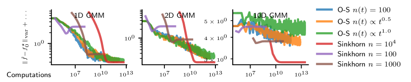
$\varepsilon=0.01$

$\varepsilon=0.001$

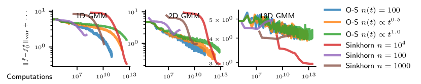
$\varepsilon=0.0001$

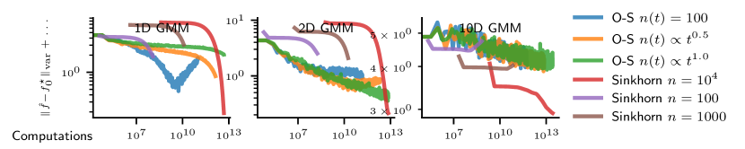
Figure 4: Performance of online Sinkhorn for various $\varepsilon$.

$\varepsilon=0.1$

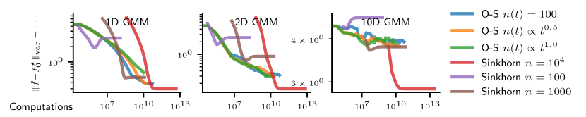
$\varepsilon=0.01$

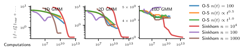
$\varepsilon=0.001$

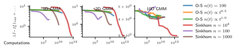
$\varepsilon=0.0001$

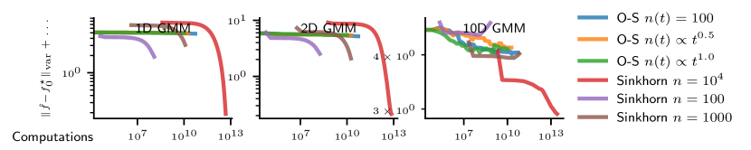
Figure 5: Performance of fully-corrective online Sinkhorn (O-S) for various $\varepsilon$.

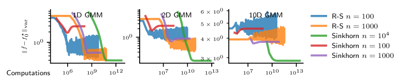
$\varepsilon=0.01$

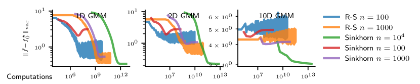
$\varepsilon=0.001$

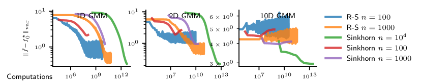
$\varepsilon=0.0001$

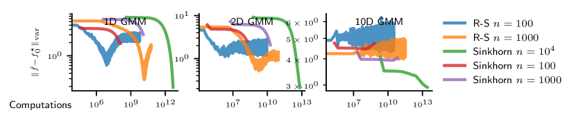
Figure 6: Performance of randomized Sinkhorn (R-S) for various $\varepsilon$.

Grids and details for §5.1.

We set $(\eta_{t},n(t))=\big{(}\frac{1}{(1+0.1t)^{a}},100(1+0.1t)^{b}\big{)}$, with $(a,b)=(0,2)$, $(a,b)=(\frac{1}{2},1)$ and $(a,b=1,0)$ (constant batch-sizes). Batch Sinkhorn algorithms uses $N=\leavevmode\nobreak\ 100,1000,10000$. We train Sinkhorn on $t=5000$ iterations, and train online Sinkhorn long enough to match the number of computations of the large Sinkhorn reference.

All OS convergence curves.

To complete Fig. 1, Fig. 4 report the performance of online Sinkhorn for $\varepsilon\in\{10^{-4},10^{-3},10^{-2},10^{-1}]\}$. The comparison of performance remains similar to the one produced in the main text.

Fully-corrective online Sinkhorn.

Fig. 5 reports the performance of fully-corrected online Sinkhorn (FCOS). We observe that the fully-corrective scheme is less noisy than the non-corrected one. It is less efficient than OS on low-dimensional problems, but faster on the 10 dimensional problem. For GMM-10D, it outperforms the batch Sinkhorn algorithm with $N=100,1000$. Note that we interrupt FCOS for $n_{t}>20,000$, as our implementation of the $C$-transform has a quadratic memory cost in $n_{t}$—this cost can be reduced to a linear cost with more careful implementation .

Randomized Sinkhorn.

Fig. 6 reports the performance of randomized Sinkhorn. In low dimension, randomized Sinkhorn is a reasonable alternative to batch Sinkhorn, as it often outperforms it on average, for the same memory complexity (compare purple to orange curve for instance). In high dimension, batch Sinkhorn tend to perform slightly better.

C.2 OT between Gaussians

We measure the performance of online Sinkhorn to transport one Gaussian distribution $\alpha$ to another $\beta$. The potentials $f^{\star},g^{\star}$ are known exactly for this problem, which allows to have a strong golden standard. More precisely, adapting the formulae from [24], assuming $\alpha\sim\mathcal{N}(\mu,A)$ and $\beta\sim\mathcal{N}(\nu,\beta)$ and writing $I$ the identity matrix in $\mathbb{R}^{d}$, we have

$$C\triangleq(AB+\frac{\varepsilon^{2}}{4}I)^{1/2},\quad U\triangleq B(C+\frac{\varepsilon}{2}I)^{-1}-I,\quad V\triangleq A(C+\frac{\varepsilon}{2}I)^{-1}-I$$ (80)

$$f^{\star}:x\to-\frac{1}{2}(x-\mu)^{\top}U(x-\mu)+x^{\top}(\mu-\nu)$$ (81)

$$g^{\star}:y\to-\frac{1}{2}(y-\nu)^{\top}V(y-\nu)+y^{\top}(\nu-\mu)$$ (82)

We compare batch Sinkhorn $(N=100,1000,10000)$ to (non fully-corrected) online Sinkhorn, with $n(t)=B$, and $n(t)=B(1+0.1t)^{1/2}$, $B=100$, and $\varepsilon\in\{10^{-4},10^{-3},10^{-2},10^{-1}\}$.

$\varepsilon=0.1$

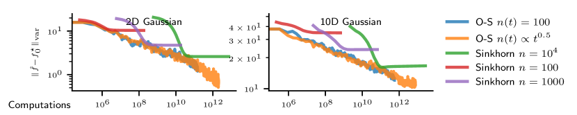
$\varepsilon=0.01$

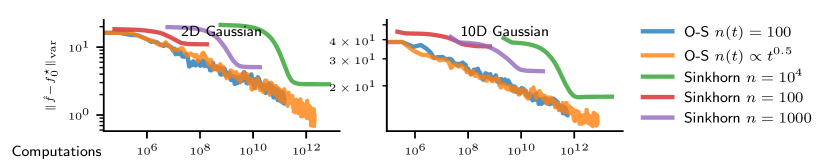
$\varepsilon=0.001$

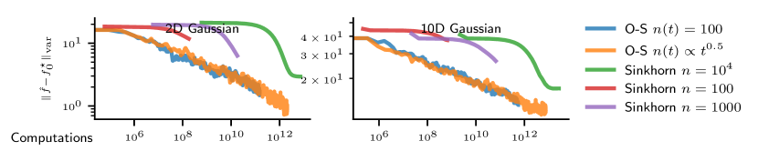
$\varepsilon=0.0001$

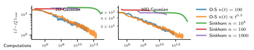
Figure 7: Performance of online-Sinkhorn to estimate OT between two Gaussians. Online Sinkhorn systematically outperforms batch Sinkhorn, but in term of speed and correction.

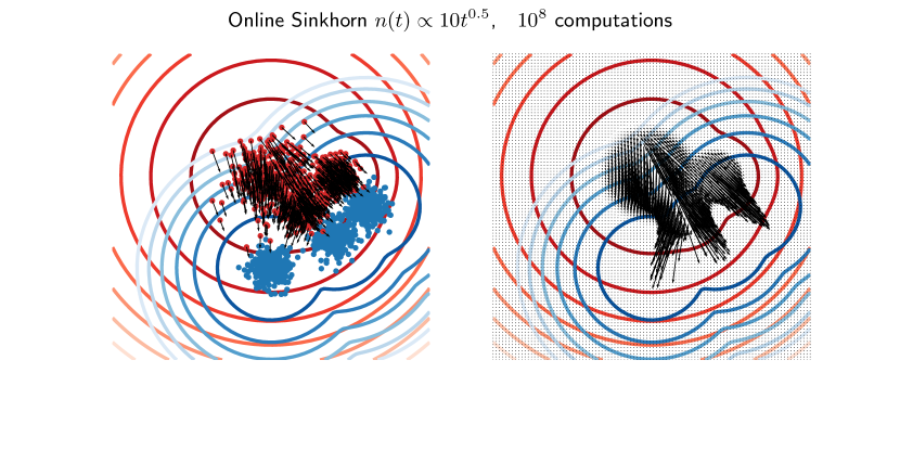
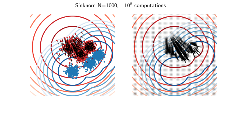
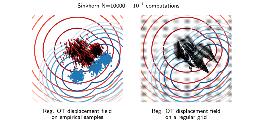
Figure 8: Displacement field as defined by the potentials estimated by online-Sinkhorn and Sinkhorn on a 2D GMM. With the same computational budget, online Sinkhorn finds smoother displacement fields than Sinkhorn. Those are closer to the true reference displacement field (we use Sinkhorn on $N=10000$ to estimate this reference). $\alpha$ and $\beta$ log-likelihood level-lines are displayed in red and blue, while the arrows are proportional to $\nabla_{x}\hat{f}_{t}(x)\textrm{d}\alpha(x)$.

Results.

As displayed in Fig. 7, online Sinkhorn outperforms batch Sinkhorn for all tested batch sizes and all $\varepsilon$. It is faster and does not converge towards biased potentials. This suggests that the performance of online Sinkhorn may be underestimated in the previous analyses due to poor potential reference.

C.3 Illustration of online Sinkhorn potentials on a 2D GMM

The estimate $\hat{f}_{t}$ is useful to compute the gradient of the Sinkhorn distance $\mathcal{W}(\alpha,\beta)$ with respect to the distribution $\alpha$. This is useful when $\alpha$ is a parametric distribution $\alpha_{\theta}$, as it allows to compute the gradient of the Sinkhorn distance with respect to $\theta$ using backpropagation. For simplicity, let us assume that $\alpha=\frac{1}{n}\sum_{i=1}^{n}\delta_{x_{i}}$. Then, for all $i\in[1,n]$,

$$\frac{\partial\mathcal{W}(\alpha,\beta)}{\partial x_{i}}=\nabla_{x}\big{(}x\to f^{\star}(\alpha,\beta)\big{)}(x_{i}),$$ (84)

so that $\nabla_{x}f^{\star}(\alpha,\beta)$ provides a displacement field that can be descended to minimize $\alpha\to\mathcal{W}(\alpha,\beta)$. Such point of view can be extended to general distributions using the mean-field point of view, see e.g. [36, 9]. Estimating $\nabla_{x}f^{\star}(\alpha,\beta)$ is therefore crucial to train e.g. generator networks. Both the online Sinkhorn and the batch Sinkhorn algorithm allow to estimate this vector field, through the plug-in estimator $x\to\nabla_{x}\hat{f}_{t}$, easily computed using the form (13) of $\hat{f}_{t}$.

Experiment.

With 2D GMMs, we estimate a reference vector field $\nabla f^{\star}_{0}$ using Sinkhorn on $N=10,000$ samples and qualitatively compare the estimations provided by online Sinkhorn and batch Sinkhorn $(N=1,000)$, for the same number of computations.

Results.

We represent the estimations $\nabla_{x}\hat{f}_{t}$ in Fig. 8, for $10^{8}$ computations. We compare them to a reference displacement field, estimated wityh $10^{1}0$ computations. We observe that online Sinkhorn estimates a smoother displacement field than batch Sinkhorn for the same computational budget, that is closer to the reference displacement field. In particular, it is less noisy in low-mass areas. This suggest that online Sinkhorn would be a interesting replacement for batch Sinkhorn in training generative architectures (used by e.g. [21]). $\alpha_{\theta}$ is then defined as the push-forward of some simple measure with a neural network $g_{\theta}$. We leave this direction for future work.

C.4 Online Sinkhorn as a warmup process

$\varepsilon=0.1$

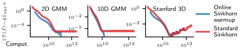
$\varepsilon=0.01$

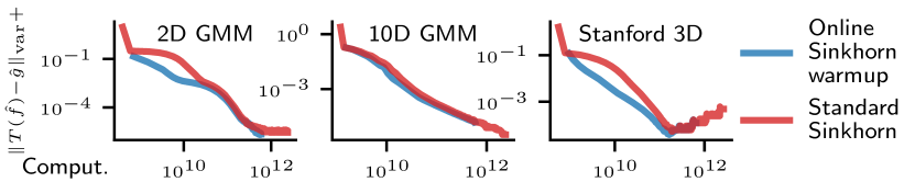
$\varepsilon=0.001$

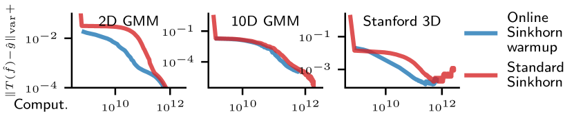
$\varepsilon=0.0001$

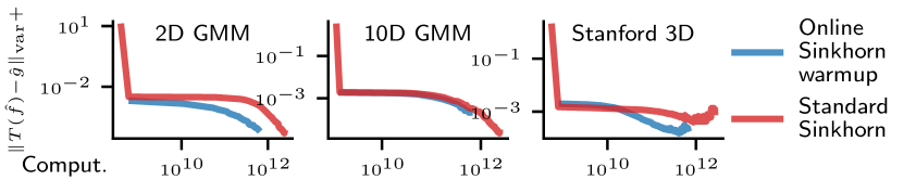
Figure 9: Performance of online-Sinkhorn as warmup for various $\varepsilon$.

Grids and details for §5.2.

We set $(\eta_{t},n(t))=\big{(}\frac{1}{(1+0.1t)^{a}},100(1+0.1t)^{b}\big{)}$, with $(a,b)=(0,2)$, $(a,b)=(\frac{1}{2},1)$ and $(a,b=1,0)$ (constant batch-sizes). The batch Sinkhorn algorithm that is used for reference and after warmup uses $N=10000$. In the reference algorithm, we precompute the distance matrix to save computation. In the warmup algorithm, this distance matrix is filled progressively and then kept in memory to perform $C$-transforms.

We evaluated OS and fully-corrective OS, and found that fully-corrective was less efficient (due to its higher cost in the early iterations). We evaluated sampling with and without replacement in the warmup phase, and found sampling without replacement to be more efficient.

All warmup convergence curves.

To complete Fig. 3, we report convergence curves for different $\varepsilon$ in Fig. 9. We find that speed-up increased with $\varepsilon$ and both the 2D and 3D problems, but remains limited for the 10D problem.

Appendix D Stochastic mirror descent interpretation

The online Sinkhorn can be understood as a stochastic mirror descent algorithm for a non-convex problem. This equivalence is obtained by applying a change of variable in (2), defining

$$\mu\triangleq\alpha\exp(f)\quad\text{and}\quad\nu\triangleq\beta\exp(g).$$ (85)

The dual problem (3) rewrites as a minimisation problem over positive measures on $\mathcal{X}$ and $\mathcal{Y}$:

$$-\!\!\!\!\min_{(\mu,\nu)\in\mathcal{M}^{+}(\mathcal{X})^{2}}\!\!\!\textrm{KL}(\alpha|\mu)+\textrm{KL}(\beta|\nu)+\langle\mu\otimes\nu,\,e^{-C}\rangle-1,$$ (86)

where the function $\textrm{KL}:\mathcal{P}(\mathcal{X})\times\mathcal{M}^{+}(\mathcal{X})\triangleq\langle\alpha,\,\log\frac{\textrm{d}\alpha}{\textrm{d}\mu}\rangle$ is the Kullback-Leibler divergence between $\alpha$ and $\mu$. This objective is block convex in $\mu$, $\nu$, but not jointly convex. As we now detail, this problem can be solved using a stochastic mirror descent [4], applied here over the Banach space of Radon measures on $\mathcal{X}$, equipped with the total variation norm.

Mirror maps and gradient.

For this, we define the (convex) distance generating function $\mathcal{M}^{+}(\mathcal{X})^{2}\to\mathbb{R}$:

$$\omega(\mu,\nu)\triangleq\textrm{KL}(\alpha|\mu)+\textrm{KL}(\beta|\nu).$$ (87)

The gradient of this function and of its Fenchel conjugate $\omega^{\star}:\mathcal{C}(\mathcal{X})^{2}\to\mathbb{R}$ yields two mirror maps. For all $(\mu,\nu)\in\mathcal{M}^{+}(\mathcal{X})^{2}$, $(\varrho,\varphi)\in\mathcal{C}(\mathcal{X})^{2},\varrho<0,\varphi<0$,

$$\nabla\omega(\mu,\nu)=(-\frac{\textrm{d}\alpha}{\textrm{d}\mu},-\frac{\textrm{d}\beta}{\textrm{d}\nu})\qquad\nabla\omega^{\star}(\varrho,\varphi)=(-\frac{\alpha}{\varrho},-\frac{\beta}{\varphi}).$$ (88)

The gradient $\nabla F(\mu,\nu)$ of the objective $F$ appearing in (86) is a continuous function

$$\nabla_{\mu}F(\mu,\nu)=-\frac{1}{\frac{\textrm{d}\mu}{\textrm{d}\alpha}}+\int_{y\in\mathcal{X}}\frac{\textrm{d}\nu}{\textrm{d}\beta}(y)\exp(-C(\cdot,y))\textrm{d}\beta(y)$$ (89)

and similarly for $\nabla_{\nu}F$.

Stochastic mirror descent.

To define stochastic mirror descent iterations, we may replace integration over $\beta$ is by an integration over a sampled measure $\hat{\beta}$. This in turn defines an unbiased gradient estimate $\tilde{\nabla}F$ of $\nabla F$, which has bounded second order moments. This absence of bias is crucial to prove convergence of SMD with high probability. Using the mirror maps and the stochastic estimation of the gradient, one has the following equivalence result, whose proofs stems from direct computations.

Proposition 7.

The stochastic mirror descent iterations

$$(\mu_{t},\nu_{t})=\nabla\omega^{\star}\Big{(}\nabla\omega(\mu_{t},\nu_{t})-\eta_{t}\tilde{\nabla}F(\mu_{t},\nu_{t})\Big{)}$$ (90)

are equal to the updates (11) under the change of variable (85).

Interpretation.

It is important to realize that $\mu_{t}$ and $\nu_{t}$ do not need to be stored in memory. Instead, their associated potentials $f_{t}$ and $g_{t}$ are parametrized as (13). In particular, $\mu_{t}$ and $\nu_{t}$ remain absolutely continuous with respect to $\alpha$ and $\beta$ respectively, so that the Kullbach-Leibler divergence terms are always finite. Note that the mirror descent we consider operates in an infinite-dimensional space, as in [23].

Finally, we mention that when computing exact gradients (in the absence of noise) and when using constant step-size of $\eta_{t}=1$, the algorithm matches exactly Sinkhorn iterations with simultaneous updates of the dual variables. This provides a novel interpretation on the Sinkhorn algorithm, that differs from the usual Bregman projection [5], and the related understanding of Sinkhorn as a constant step-size mirror descent on the primal objective [32] and on a semi-dual formulation [27].

Note that one can not directly apply the proofs of convergence of mirror descent to our problem, as the lack of convexity of problem (86) prevents their use.

References

- [1] Ya.. Alber, C.. Chidume and Jinlu Li “Stochastic Approximation Method for Fixed Point Problems” In Applied Mathematics 03.12, 2012, pp. 2123–2132
- [2] Jason Altschuler, Jonathan Niles-Weed and Philippe Rigollet “Near-linear time approximation algorithms for optimal transport via Sinkhorn iteration” In Advances in Neural Information Processing Systems, 2017
- [3] Martin Arjovsky, Soumith Chintala and Léon Bottou “Wasserstein Generative Adversarial Network” In Proceedings of the International Conference on Machine Learning, 2017
- [4] Amir Beck and Marc Teboulle “Mirror descent and nonlinear projected subgradient methods for convex optimization” In Operations Research Letters 31.3 Elsevier, 2003, pp. 167–175
- [5] Jean-David Benamou, Guillaume Carlier, Marco Cuturi, Luca Nenna and Gabriel Peyré “Iterative Bregman projections for regularized transportation problems” In SIAM Journal on Scientific Computing 37.2 SIAM, 2015, pp. A1111–A1138
- [6] Leo Breiman “The Strong Law of Large Numbers for a Class of Markov Chains” In The Annals of Mathematical Statistics 31.3, 1960, pp. 801–803
- [7] Guillermo Canas and Lorenzo Rosasco “Learning probability measures with respect to optimal transport metrics” In Advances in Neural Information Processing Systems, 2012
- [8] Gilles Celeux and Jean Diebolt “A stochastic approximation type EM algorithm for the mixture problem” In Stochastics and Stochastic Reports 41.1, 1992, pp. 119–134
- [9] Lenaic Chizat “Sparse Optimization on Measures with Over-parameterized Gradient Descent” In arXiv preprint arXiv:1907.10300v1, 2019
- [10] Nicolas Courty, Rémi Flamary, Devis Tuia and Alain Rakotomamonjy “Optimal transport for domain adaptation” In IEEE Transactions on Pattern Analysis and Machine Intelligence 39.9 IEEE, 2016, pp. 1853–1865
- [11] Marco Cuturi “Sinkhorn Distances: Lightspeed Computation of Optimal Transport” In Advances in Neural Information Processing Systems, 2013
- [12] Marco Cuturi and Gabriel Peyré “Semidual Regularized Optimal Transport” In SIAM Review 60.4 SIAM, 2018, pp. 941–965
- [13] Arnak S Dalalyan and Avetik Karagulyan “User-friendly guarantees for the Langevin Monte Carlo with inaccurate gradient” In Stochastic Processes and their Applications 129.12 Elsevier, 2019, pp. 5278–5311
- [14] Persi Diaconis and David Freedman “Iterated random functions” In SIAM Review 41.1 SIAM, 1999, pp. 45–76
- [15] R.. Dudley “The Speed of Mean Glivenko-Cantelli Convergence” In The Annals of Mathematical Statistics 40.1, 1969, pp. 40–50
- [16] Kilian Fatras, Younes Zine, Rémi Flamary, Rémi Gribonval and Nicolas Courty “Learning with minibatch Wasserstein: asymptotic and gradient properties” In arXiv preprint arXiv:1910.04091, 2019
- [17] Jean Feydy, Thibault Séjourné, François-Xavier Vialard, S. Amari, Alain Trouvé and Gabriel Peyré “Interpolating between Optimal Transport and MMD using Sinkhorn Divergences” In International Conference on Artificial Intelligence and Statistics, 2019
- [18] Charlie Frogner, Chiyuan Zhang, Hossein Mobahi, Mauricio Araya and Tomaso A Poggio “Learning with a Wasserstein loss” In Advances in Neural Information Processing Systems, 2015
- [19] Aude Genevay, Lenaic Chizat, Francis Bach, Marco Cuturi and Gabriel Peyré “Sample Complexity of Sinkhorn divergences” In International Conference on Artificial Intelligence and Statistics, 2019
- [20] Aude Genevay, Marco Cuturi, Gabriel Peyré and Francis Bach “Stochastic Optimization for Large-scale Optimal Transport” In Advances in Neural Information Processing Systens, 2016, pp. 3432–3440
- [21] Aude Genevay, Gabriel Peyré and Marco Cuturi “Learning Generative Models with Sinkhorn Divergences” In International Conference on Artificial Intelligence and Statistics, 2018, pp. 1608–1617
- [22] Andrew V Goldberg and Robert E Tarjan “Finding minimum-cost circulations by canceling negative cycles” In Journal of the ACM 36.4, 1989, pp. 873–886
- [23] Ya-Ping Hsieh, Chen Liu and Volkan Cevher “Finding Mixed Nash Equilibria of Generative Adversarial Networks” In arXiv preprint arXiv:1811.02002, 2018
- [24] Hicham Janati, Boris Muzellec, Gabriel Peyré and Marco Cuturi “Entropic Optimal Transport between (Unbalanced) Gaussian Measures has a Closed Form” In arXiv:2006.02572 [math, stat], 2020 arXiv:2006.02572
- [25] L. Kantorovich “On the transfer of masses (in Russian)” In Doklady Akademii Nauk 37.2, 1942, pp. 227–229
- [26] Simon Lacoste-Julien and Martin Jaggi “On the global linear convergence of Frank-Wolfe optimization variants” In Advances in Neural Information Processing Systems, 2015
- [27] Flavien Léger “A gradient descent perspective on Sinkhorn” In arXiv preprint arXiv:2002.03758, 2019
- [28] Bas Lemmens and Roger Nussbaum “Nonlinear Perron–Frobenius Theory” Cambridge: Cambridge University Press, 2012
- [29] Julien Mairal “Stochastic majorization-minimization algorithms for large-scale optimization” In Advances in Neural Information Processing Systems, 2013
- [30] Arthur Mensch, Mathieu Blondel and Gabriel Peyré “Geometric Losses for Distributional Learning” In Proceedings of the International Conference on Machine Learning, 2019
- [31] Quentin Mérigot “A multiscale approach to optimal transport” In Computer Graphics Forum 30.5, 2011, pp. 1583–1592 Wiley Online Library
- [32] Konstantin Mishchenko “Sinkhorn Algorithm as a Special Case of Stochastic Mirror Descent” In arXiv preprint arXiv:1909.06918, 2019
- [33] Eric Moulines and Francis Bach “Non-Asymptotic Analysis of Stochastic Approximation Algorithms for Machine Learning” In Advances in Neural Information Processing Systems, 2011, pp. 451–459
- [34] Gabriel Peyré and Marco Cuturi “Computational optimal transport” In Foundations and Trends® in Machine Learning 11.5-6 Now Publishers, Inc., 2019, pp. 355–607
- [35] Herbert Robbins and Sutton Monro “A stochastic approximation method” In The Annals of Mathematical Statistics, 1951, pp. 400–407
- [36] Filippo Santambrogio “Optimal transport for applied mathematicians” In Birkäuser, NY 55.58-63 Springer, 2015, pp. 94
- [37] Vivien Seguy, Bharath Bhushan Damodaran, Rémi Flamary, Nicolas Courty, Antoine Rolet and Mathieu Blondel “Large-scale optimal transport and mapping estimation” In International Conference on Learning Representations, 2018
- [38] Richard Sinkhorn “A relationship between arbitrary positive matrices and doubly stochastic matrices” In The Annals of Mathematical Statistics 35, 1964, pp. 876–879
- [39] Richard Sinkhorn and Paul Knopp “Concerning nonnegative matrices and doubly stochastic matrices” In Pacific Journal of Mathematics 21.2 Mathematical Sciences Publishers, 1967, pp. 343–348
- [40] Matthew Staib, Sebastian Claici, Justin M Solomon and Stefanie Jegelka “Parallel streaming Wasserstein barycenters” In Advances in Neural Information Processing Systems, 2017
- [41] Greg Turk and Marc Levoy “Zippered polygon meshes from range images” In Proceedings of the 21st annual conference on Computer graphics and interactive techniques, 1994, pp. 311–318
- [42] Aad W. Van der Vaart “Asymptotic statistics” Cambridge University Press, 2000
- [43] François-Xavier Vialard “An elementary introduction to entropic regularization and proximal methods for numerical optimal transport”, 2019
- [44] Jonathan Weed and Francis Bach “Sharp asymptotic and finite-sample rates of convergence of empirical measures in Wasserstein distance” In Bernoulli 25.4A Bernoulli Society for Mathematical StatisticsProbability, 2019, pp. 2620–2648