Does the spin tensor play any role in non-gravitational physics?

Abstract

In view of the recent polarization measurements in ultra-relativistic heavy ion collisions, we discuss the possibility of a physical meaning of the spin angular momentum in quantum field theory and relativistic hydrodynamics.

1 Introduction

The evidence of a finite global polarization of particles in relativistic heavy-ion collisions [1] has opened a new perspective in the field as well as in the theory of relativistic matter. While the experiments proved to be able to measure polarization differentially in momentum space [2], theoretical predictions are mostly based on local thermodynamic equilibrium, which imply a relation between spin and thermal vorticity [3]. In fact, this relation has been recently questioned based on the idea that the separation between orbital and spin angular momentum in quantum physics is possibly physically meaningful. In this case, the spin of the particles would not be necessarily related to thermal vorticity [4, 5]. In gravitational physics, the stress-energy tensor and the spin tensor (Einstein-Cartan theory) have an objective physical meaning, because they are related to the local geometry of space-time. Beyond gravitational theories, the problem of the physical significance of the spin tensor beyond is a long-standing one [6] and has been rediscussed more recently in e.g. ref. [7], where it was demonstrated that, e.g. that some quantities such as viscosity change by small quantum terms depending on whether a spin tensor is there. In this work, which is largely based on ref. [8], I will delve into this subject and the possible phenomenological implications.

2 Spin tensor and pseudo-gauge transformations

In relativistic quantum field theory in flat space-time, according to Noether’s theorem, for each continuous symmetry of the action, there is a corresponding conserved current. The currents associated with the translational symmetry and the Lorentz symmetry are the so-called canonical stress-energy tensor and the canonical angular momentum tensor:

$${\widehat{T}}^{\mu\nu}_{C}=\sum_{a}\frac{\partial\cal L}{\partial(\partial_{\mu}{\widehat{\psi}}^{a})}\partial^{\nu}{\widehat{\psi}}^{a}-g^{\mu\nu}{\cal L},\qquad\qquad\widehat{\cal J}^{\mu,\lambda\nu}_{C}=x^{\lambda}{\widehat{T}}^{\mu\nu}_{C}-x^{\nu}{\widehat{T}}^{\mu\lambda}_{C}+{\widehat{\cal S}}^{\mu,\lambda\nu}_{C}.$$ (1)

In eq. (1), ${\cal L}$ is the lagrangian density, while ${\widehat{\cal S}}_{C}$ reads

$${\widehat{\cal S}}^{\mu,\lambda\nu}_{C}=-i\sum_{a,b}\frac{\partial\cal L}{\partial(\partial_{\mu}{\widehat{\psi}}^{a})}D(J^{\lambda\nu})^{a}_{b}{\widehat{\psi}}^{b}$$ (2)

with $D$ being the irreducible representation matrix of the Lorentz group pertaining to the field. The above tensors fulfill the following equations:

$$\nabla_{\mu}{\widehat{T}}^{\mu\nu}_{C}=0,\qquad\nabla_{\mu}\widehat{\cal J}^{\mu,\lambda\nu}_{C}={\widehat{T}}^{\lambda\nu}_{C}-{\widehat{T}}^{\nu\lambda}_{C}+\nabla_{\mu}{\widehat{\cal S}}^{\mu,\lambda\nu}_{C}=0,$$ (3)

It turns out, however, that the stress-energy and angular momentum tensors are not uniquely defined. Different pairs can be generated either by just changing the lagrangian density or, more generally, by means of the so-called pseudo-gauge transformations [6]:

$${\widehat{T}}^{\prime\mu\nu}={\widehat{T}}^{\mu\nu}+\frac{1}{2}\nabla_{\lambda}\left({\widehat{\Phi}}^{\lambda,\mu\nu}-{\widehat{\Phi}}^{\mu,\lambda\nu}-{\widehat{\Phi}}^{\nu,\lambda\mu}\right),$$

$${\widehat{\cal S}}^{\prime\lambda,\mu\nu}={\widehat{\cal S}}^{\lambda,\mu\nu}-{\widehat{\Phi}}^{\lambda,\mu\nu},$$ (4)

where ${\widehat{\Phi}}$ is a rank-three tensor field antisymmetric in the last two indices, often called and henceforth referred to as superpotential. In Minkowski space-time, the newly defined tensors preserve the total energy, momentum, and angular momentum (herein expressed in Cartesian coordinates):

$${\widehat{P}}^{\nu}=\int_{\Sigma}{\rm d}\Sigma_{\mu}{\widehat{T}}^{\mu\nu},\qquad{\widehat{J}}^{\lambda\nu}=\int_{\Sigma}{\rm d}\Sigma_{\mu}\widehat{\cal J}^{\mu,\lambda\nu},$$ (5)

as well as the conservation equations (3) .

A special pseudo-gauge transformation is the one where one starts with the canonical definitions and the superpotential is the spin tensor itself, that is, ${\widehat{\Phi}}={\widehat{\cal S}}$. In this case, the new spin tensor vanishes, ${\widehat{\cal S}}^{\prime}=0$, and the new stress-energy tensor is the so-called Belinfante stress-energy tensor ${\widehat{T}}_{B}$,

$${\widehat{T}}^{\mu\nu}_{B}={\widehat{T}}^{\mu\nu}_{C}+\frac{1}{2}\nabla_{\lambda}\left({\widehat{\cal S}}^{\lambda,\mu\nu}_{C}-{\widehat{\cal S}}^{\mu,\lambda\nu}_{C}-{\widehat{\cal S}}^{\nu,\lambda\mu}_{C}\right).$$ (6)

It is common wisdom in Quantum Field Theory that no actual physical measurement can be made in flat space-time discriminating between different couples of stress-energy and spin tensor; in other words, no measurement can depend on the superpotential. This is effectively rephrased in the adage it is impossible to separate orbital angular momentum and spin. One should be a little more specific: when saying ”no actual physical measurement” direct measurements of the energy-momentum density, which are obviously sensitive to the superpotential according to eq. (2), are not included. Indeed, space-time local measurement is not possible in a high energy physics experiment and in heavy ion collisions as well. Upon some reflection, one can realized that any measurement involves particles in momentum space and momentum spectra are supposedly independent of the pseudo-gauge transformation.

We can reinforce the above argument by saying that the stress-energy tensor, being a pseudo-gauge dependent quantity, is not a physical object; it is defined, and can be probed with particle measurements, only up to quantum corrections encoded in the superpotential ${\widehat{\Phi}}$. This might be the end of the story, however we are going to see that something more can be told.

3 States, operators and local equilibrium

In quantum physics, there are operators and states. Operators can be invariant under some transformation; for instance, the operators in (5) are invariant under the transformation (2). On the other hand, quantum states can either be invariant under the same transformation or they can not. This dichotomy is reminiscent of the general definition of spontaneous symmetry breaking: while the action of a quantum field theory is invariant under some transformation of the fields, the vacuum state is not. Similarly, within our scope, we can conceive a quantum states which are not invariant under a pseudo-gauge transformations. In principle, this is a very easy operation; take a free field theory, whose Hilbert space basis states are defined by a set of number of occupations for each momentum $p$ and spin state $s$:

$$|\{n\}_{p,s}\rangle$$

These states, being eigenstates of the four-momentum, are clearly pseudo-gauge invariant. Nevertheless, a pseudo-gauge-dependent state can be generated by just forming a linear superposition of the above state with complex coefficients which functionally depend on a particular superpotential $\Phi$ in eq. (2), once a reference set is chosen (e.g. Belinfante):

$$|{\rm state}\rangle=\sum C[\Phi]_{\{n\}_{p,s}}|\{n\}_{p,s}\rangle$$ (7)

This can be easily extended to a mixed state and its associated density operator ${\widehat{\rho}}$. Hence, if the density operator depends on the superpotential, so will the mean values of any quantum operator $\widehat{O}$, whether it is related to measurable quantity or not:

$$O([\Phi])={\rm tr}\left({\widehat{\rho}}[\Phi]\,\widehat{O}\right)$$

To make this concrete, we will now write down a mixed state which is very relevant for relativistic fluid, which is indeed pseudo-gauge dependent. This is the density operator describing local thermodynamic equilibrium in quantum field theory [9, 10, 11, 12]:

$${\widehat{\rho}}_{\rm LE}=\frac{1}{Z}\exp\left[-\int_{\Sigma}{\rm d}\Sigma_{\mu}\left({\widehat{T}}^{\mu\nu}_{B}\beta_{\nu}-\zeta\,{\widehat{j}}^{\mu}\right)\right],$$ (8)

where $\beta$ and $\zeta$ are the four-temperature vector and the ratio between local chemical potential and temperature respectively. The operator (8) is obtained by maximizing the entropy with the constraints [11]:

$$n_{\mu}{\rm tr}\left({\widehat{\rho}}\,{\widehat{T}}_{B}^{\mu\nu}\right)=n_{\mu}T_{B}^{\mu\nu},\qquad n_{\mu}{\rm tr}\left({\widehat{\rho}}\,{\widehat{j}}^{\mu}\right)=n_{\mu}j^{\mu}.$$ (9)

Note the use of the Belinfante’s stress-energy tensor ${\widehat{T}}_{B}$ in both eqs. (8) and (9); in this case, angular momentum density constraints are redundant because the associated spin tensor vanishes [8]. Note that the operator (8) is not the actual density operator, because it is not generally stationary as required in the Heisenberg picture. In fact, the true density operator for a system achieving local thermodynamic equilibrium is the one in eq. (8) for some 3D hypersurface at the time $\tau_{0}$, that is $\Sigma(\tau_{0})$ [9] (see also discussion in ref. [13]).

One can now use the pseudo-gauge transformations of Sec. 2 to rewrite the local thermodynamic equilibrium density operator as a function of, e.g., canonical tensors. Using eq. (6),

$${\widehat{\rho}}_{\rm LE}=\frac{1}{Z}\exp\left[-\int_{\Sigma}{\rm d}\Sigma_{\mu}\left({\widehat{T}}^{\mu\nu}_{C}\beta_{\nu}-\frac{1}{2}\varpi_{\lambda\nu}{\widehat{\cal S}}^{\mu,\lambda\nu}_{C}-\frac{1}{2}\xi_{\lambda\nu}\left({\widehat{\cal S}}^{\lambda,\mu\nu}_{C}+{\widehat{\cal S}}^{\nu,\mu\lambda}_{C}\right)-\zeta{\widehat{j}}^{\mu}\right)\right],$$ (10)

where

$$\varpi_{\lambda\nu}=\frac{1}{2}(\nabla_{\nu}\beta_{\lambda}-\nabla_{\lambda}\beta_{\nu})\qquad\qquad\xi_{\lambda\nu}=\frac{1}{2}(\nabla_{\nu}\beta_{\lambda}+\nabla_{\lambda}\beta_{\nu})$$ (11)

are the thermal vorticity and the symmetric part of the gradient of the four-temperature vector, what can be called thermal shear tensor.

Had we used another couple of tensors, instead of Belinfante, to calculate the local thermodynamic equilibrium operator, the operator would be different. The inclusion of angular momentum density amongst the constraints defining local thermodynamic equilibrium implies an additional constraint:

$$n_{\mu}{\rm tr}\left({\widehat{\rho}}\,{\widehat{\cal S}}^{\mu,\lambda\nu}\right)=n_{\mu}{\cal S}^{\mu,\lambda\nu}.$$ (12)

and the introduction of an additional antisymmetric tensor field $\Omega_{\lambda\nu}$ as Lagrange multiplier for the equation (12), the spin potential. The associated local equilibrium density operator is:

$${\widehat{\rho}}_{\rm LE}=\frac{1}{Z}\exp\left[-\int_{\Sigma}{\rm d}\Sigma_{\mu}\left({\widehat{T}}^{\mu\nu}\beta_{\nu}-\frac{1}{2}\Omega_{\lambda\nu}{\widehat{\cal S}}^{\mu,\lambda\nu}-\zeta{\widehat{j}}^{\mu}\right)\right].$$ (13)

If ${\widehat{T}}={\widehat{T}}_{C}$ and ${\widehat{\cal S}}={\widehat{\cal S}}_{C}$, 5he operator (13) is the same as (10) (hence (8)) if $\beta$ and $\zeta$ are the same fields, $\Omega=\varpi$ and $\xi=0$. The latter condition implies that the equilibrium should be global [14] for the two operators to coincide. Otherwise, they do not; the operator is pseudo-gauge dependent and we are in a situation like the one described by the eq. (7) for a pure state.

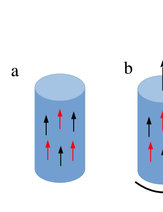
Fig. 1: (Color online) a) a macroscopic fluid at rest with polarized particles (black arrows) and antiparticles (red arrows) b) if the spin tensor vanishes, the fluid must be rotating (non-vanishing thermal vorticity) to have polarized particles and antiparticles in the same direction.

To get an insight of which state an operator (13) can describe that cannot be described by the eq. (8), one can envisage a fluid temporarily at rest with a constant temperature $T$, hence $\beta=(1/T)(1,{\bf 0})$, wherein both particles and antiparticles are polarized in the same direction (see Fig. 1). Such a situation cannot be described as local thermodynamic equilibrium by the density operator (8) because the only way to get particles and antiparticles polarized, in this case, is through a non-vanishing thermal vorticity, that is when the fluid rotates. Yet, thermal vorticity vanishes if $\beta$ is constant, so only through a non-vanishing spin potential $\Omega$ is a charge-independent polarization (such as that observed in the experiment [1]) possible.

Indeed, polarization is the most sensitive variable to discriminate between the two local equilibria density operators. It is thus very important to understand whether the data can be accomodated within the Belinfante LEQ description (8) or whether an extension of hydrodynamics to include the spin potential is needed. The latter option is under scrutiny [15]. For an ampler discussion we refer the reader to ref. [8].

References

- [1] L. Adamczyk et al. [STAR Collaboration], Nature 548 (2017) 62.
-
[2]
J. Adam et al. [STAR Collaboration],
Phys. Rev. C 98 (2018) 014910;
J. Adam et al. [STAR Collaboration], Phys. Rev. Lett. 123 (2019) no.13, 132301. - [3] F. Becattini, V. Chandra, L. Del Zanna and E. Grossi, Annals Phys. 338 (2013) 32.
- [4] W. Florkowski, B. Friman, A. Jaiswal and E. Speranza, Phys. Rev. C 97 (2018) no.4, 041901;
- [5] W. Florkowski, R. Ryblewski and A. Kumar, Prog. Part. Nucl. Phys. 108 (2019) 103709.
- [6] F. W. Hehl, Rept. Math. Phys. 9, 55 (1976).
- [7] F. Becattini and L. Tinti, Phys. Rev. D 87 (2013) no.2, 025029.
- [8] F. Becattini, W. Florkowski and E. Speranza, Phys. Lett. B 789 (2019) 419.
- [9] D. N. Zubarev, Sov. Phys. Doklady 10, 850 (1966); D. N. Zubarev, A. V. Prozorkevich, S. A. Smolyanskii, Theoret. and Math. Phys. 40 (1979), 821.
- [10] Ch. G. Van Weert, Ann. Phys. 140, 133 (1982).
- [11] F. Becattini, L. Bucciantini, E. Grossi and L. Tinti, Eur. Phys. J. C 75 (2015) no.5, 191.
- [12] M. Hongo, Annals Phys. 383 (2017) 1.
- [13] F. Becattini, M. Buzzegoli and E. Grossi, Particles 2 (2019) no.2, 197.
- [14] F. Becattini, Phys. Rev. Lett. 108 (2012) 244502.
- [15] W. Florkowski, arXiv:2002.04823 [nucl-th] and this conference.