Discrete Vortices in Systems of Coupled Nonlinear Oscillators:
Numerical Results for an Electric Model

Abstract

Vortex coherent structures on arrays of nonlinear oscillators joined by weak links into topologically nontrivial two-dimensional discrete manifolds have been theoretically studied. A circuit of nonlinear electric oscillators coupled by relatively weak capacitances has been considered as a possible physical implementation of such objects. Numerical experiments have shown that a time-monochromatic external force applied to several oscillators leads to the formation of long-lived and nontrivially interacting vortices in the system against a quasistationary background in a wide range of parameters. The dynamics of vortices depends on the method of “coupling” of the opposite sides of a rectangular array by links, which determines the topology of the resulting manifold (torus, Klein bottle, projective plane, Möbius strip, ring, or disk).

I Introduction

As known, nonlinear complex wavefields can form quantum vortices in two- and three-dimensional spaces [1-7]. A typical example is vortices in trapped Bose condensates of cold atoms (which are described by the condensate wavefunction $\Psi({\bf r},t)$ within the Gross-Pitaevskii equation). Nontrivial dynamic properties of these objects attract attention of researchers (see, e.g., [8-19]). Vortex structures exist not only in continuous media but also in discrete systems (vortices and vortex solitons on lattices; see [20-29] and references therein). Dynamic systems on lattices allow different physical and mathematical realizations. In particular, vortices in arrays of coupled nonlinear oscillators can exist because each site involves the canonical complex order parameter $a_{n}=\sqrt{S_{n}}\exp(i\Theta_{n})=A_{n}(t)\exp(-i\omega_{0}t)$ , where $S_{n}$ and $\Theta_{n}$ are the action and angle variables for a single oscillator, respectively, and $\omega_{0}$ is the frequency of oscillations in the limit of small amplitudes. The phase $\Theta$ changing slowly upon the bypass along a closed contour along the links can acquire an increment multiple of $2\pi$, thus forming a discrete vortex. However, for such an object to have a pronounced localized core and to be long-lived against a modulationally stable nonzero “density” background $S$, the effect of nonlinearity should be defocusing. The core of the vortex (dip of the density) can be in this case as narrow as about one step of the lattice and even smaller in a certain sense, but the effect of its phase covers the entire system. This property distinguishes ordinary vortices from localized vortex solitons occurring upon focused nonlinearity. The interaction of discrete vortices with each other and with sites of the lattice is responsible for the complex dynamics, which is the subject of this work.

One of the relatively simple and universal mathematical models allowing vortex solutions is the weakly dissipative discrete nonlinear Schrödinger equation with pump

$$i(\dot{A}_{n}+\gamma\omega_{0}A_{n})=g|A_{n}|^{2}A_{n}$$

$$\qquad\qquad+\frac{1}{2}\sum_{n^{\prime}}c_{n,n^{\prime}}(A_{n}-A_{n^{\prime}})+f_{n}(t),$$ (1)

where $\gamma$ is a small linear damping coefficient, $g$ is a nonlinear coefficient, $c_{n,n^{\prime}}$ is a (real) coupling matrix, and $f_{n}(t)$ is the complex envelope of an external quasimonochromatic force (near the resonance frequency). In particular, various metamaterials are described by an equation of this type (see, e.g., [30] and references). It summarizes effects of nonlinearity, dispersion, dissipation, and resonance pumping. Real possible oscillators satisfy such a universal equation only approximately and only in a weakly nonlinear regime. Consequently, Eq.(1) is insufficient for studying the possibility of fabrication of artificial materials that can demonstrate discrete vortices, and it is of interest to study strongly nonlinear physically implementable systems.

It is noteworthy that electric circuits with reverse-biased varactor diodes (variable capacitances depending on the applied voltage) are practically convenient implementations of coupled nonlinear oscillators [31-45]. In particular, they were used to perform experiments simulating the dynamics of solitons on an integrable Toda chain [31-34]. In addition to diodes, nonlinear capacitors based on special dielectric films have also been developed [46,47].

Depending on the design of a circuit, nonlinearity can be both focusing at large scales and defocusing. Until now, focusing variants characterized by the modulation instability of long waves have primarily been studied for discrete solitons, breathers, and vortex solitons [20,22,42,43]. These strongly localized structures are formed on modulationally unstable networks even with small sizes (smaller than $10\times 10$) and occupy only a few cells [43]. Unlike them, the reliable observation of vortices on modulationally stable arrays of coupled oscillators requires a large number of elements, at least $30\times 30$, because the spatial distribution of the phases of vortices is usually delocalized. The fabrication of such large arrays requires high costs. This is likely why vortices on networks have not yet been observed experimentally. An interesting fact that systems of electric oscillators allow such design of couplings that provides topologically nontrivial discrete manifolds, e.g., Möbius strip, Klein bottle, and projective plane, still does not attract attention. Since vortices are long-range objects, the topology of manifolds should strongly affect them. As far as I know, the dynamics of discrete vortices on complex manifolds has not yet been studied (in contrast to discrete solitons on a quasi-one-dimensional Möbius strip [48]). The aim of this work is to partially fill this gap by only the numerical simulation of a fairly realistic electric model. As will be seen below, already the first results appear to be nontrivial and interesting. In particular, long-lived vortices on a discrete weakly dissipative electric circuit under a periodic external action in the nonlinear resonance regime are observed in a numerical experiment for the first time.

Figure 1: Circuit of coupled nonlinear electric oscillators. Only a fragment of the entire circuit (two cells and a link between them) is shown.

II Description of the model

Figure 1 shows the considered circuit consisting of nonlinear electric oscillators coupled by relatively weak capacitive couplings between them. The relation between this circuit and Eq.(1) was recently discussed in [45]. A state of the system is described by voltages $V_{n}(t)$ and by currents $I_{n}(t)$ through inductors $L$ toward the corresponding capacitor. The use of toroidal coils is suggested in order to exclude mutual induction. Here, capacitors $C(V_{n})$ are nonlinear elements. For simplicity, the voltage dependence of the capacitance is used in the form

$$C(V_{n})=C_{0}(1+V_{n}^{2}/V_{*}^{2}),$$ (2)

where $V_{*}$ is a parameter of about several volts. This symmetric dependence is characteristic of capacitors with dielectric films [46, 47]. The application of the bias voltage $V_{b}$ makes it possible to use also varicaps, which (in parallel connection to a normal capacitor) are approximately described by the formula (see, e.g.,[49])

$$C(V_{n})=C_{0}\Big{[}\mu+(1-\mu)/(1+V_{n}/V_{*})^{\nu}\Big{]},$$ (3)

where $0<\mu<1$ is a parameter taking into account the normal capacitor connected in parallel and $\nu$ is a fitting parameter of the diode, which depends on the technology of fabrication and is usually in the range of $0.3\lesssim\nu\lesssim 6.0$ ($\nu=1$ should be taken to obtain a Toda chain). In any case, the stored electrostatic energy on the capacitor (additional to that in the state $V_{n}=0$ ) is determined by the formula

$$W(V_{n})={\textstyle\int}_{0}^{V_{n}}C(u)udu,$$ (4)

and the additional electric charge is

$$q_{n}=q(V_{n})={\textstyle\int}_{0}^{V_{n}}C(u)du.$$ (5)

All capacitances $C_{n,n^{\prime}}$ on couplings are assumed to be linear and small compared to $C_{0}$. Generally speaking, couplings are not necessarily identical, which allows an additional degree of freedom in the design of networks with spatially inhomogeneous properties. It is possible to fabricate locally periodic, quasicrystalline, and (pseudo)random lattices.

Under the assumption that connecting wires have negligibly small resistances, inductances, and capacitances, the real spatial arrangement of the elements of the circuit is insignificant. Circuits with almost any topology are obviously implementable because of the flexibility and small cross section of wires.

For the electric model to be realistic, it should include dissipative elements such as a low active resistance of the coil $R_{L}\ll\sqrt{L/C_{0}}$ and high leakage resistances of capacitors $R_{C}\gg\sqrt{L/C_{0}}$ and $R_{n,n^{\prime}}\gg\sqrt{L/C_{0}}$. For simplicity, a possible nonlinear dependence of $R_{C}$ on the voltage applied to the capacitor is ignored. Furthermore, to compensate energy losses in the system, an alternating voltage ${\cal E}_{n}(t)$ (generator connected in series to the coil is not shown in Fig.1) is applied to a few oscillators.

In the general case, the steady-state voltage on the capacitor is slightly different from $V_{b}$ because of the finiteness of $R_{C}$, but this difference can be neglected in the measure of a very small parameter $R_{L}/R_{C}$. Then, the system of equations of motion has the form

$$C(V_{n})\dot{V}_{n}+\sum_{n^{\prime}}\big{[}C_{n,n^{\prime}}(\dot{V}_{n}-\dot{V}_{n^{\prime}})$$

$$\qquad\qquad+(V_{n}-V_{n^{\prime}})/R_{n,n^{\prime}}\big{]}+V_{n}/R_{C}=I_{n},$$ (6)

$$L\dot{I}_{n}+V_{n}+R_{L}I_{n}={\cal E}_{n}(t).$$ (7)

To solve this system with respect to the time derivatives $\dot{V}_{n}$ in the numerical algorithm, it is possible to use iterations corresponding to the Euler scheme for relaxation to the equilibrium position. In this case, the convergence of iterations is ensured by the symmetry and positive definiteness of the matrix $\{[C(V_{n})+\sum_{m}C_{n,m}]\delta_{n,n^{\prime}}-C_{n,n^{\prime}}\}$ appearing in Eq.(6). The result of iterations is then substituted into a 4th-order Runge-Kutta algorithm for time evolution. The calculations are performed in dimensionless variables $L=1$, $C_{0}=1$, and $V_{*}=1$. Correspondingly, the frequency and period of small oscillations are $\omega_{0}=1$ and $T_{0}=2\pi$ , respectively. It is noteworthy that the energy $\varepsilon_{n}=LI_{n}^{2}/2+W(V_{n})$ of each oscillator in the absence of couplings and dissipation would be conserved.

The requirement that the nonlinear frequency shift $\delta\omega_{\rm nl}=g|A|^{2}$ of a separate oscillator be negative is fundamentally important because, as shown in [45], the dominant elements of the matrix $c_{n,n^{\prime}}$ of the corresponding equation (1) are negative, although the energy of couplings in our model is positive definite. It is particularly easy to test this by the example of an infinite square lattice by calculating the dispersion law for the linearized system and verifying that the quadratic correction to the frequency at low wavenumbers is negative. When the signs of the nonlinear coefficient and dispersion correction are the same, the action of nonlinearity will be defocusing in the quasi-continuum limit, which is necessary for the formation of a stable background on which vortices exist. This condition with the function (2) is satisfied automatically (because $g=-1/4$ in this case) and with the function (3) is satisfied in the region of the parameters

$$g=\nu(1-\mu)[-3+\nu(1-4\mu)]/24<0.$$ (8)

It is assumed that dissipation in the coil prevails over leakage dissipation, so that the Q-factor of a separate oscillator

$$Q^{-1}=\gamma=\left(R_{L}\sqrt{C_{0}/L}+R_{C}^{-1}\sqrt{L/C_{0}}\right)/2$$ (9)

is determined primarily by the first term. The numerical experiments show that a high Q-factor $Q\gtrsim 10^{3}$ is required for the observation of vortices. This requirement seems quite realistic. In particular, for the coil with the inductance $L=1.0\times 10^{-4}$ H and resistance $R_{L}=1\,\Omega$ (such a coil made of a wire with a length of 10 m and a cross section of 0.2 mm² has dimensions of several centimeters) at the values $C_{0}=1.0\times 10^{-10}$ F and $R_{C}>10^{7}\,\Omega$, we obtain $\omega_{0}=1.0\times 10^{7}$ rad/s (corresponding to a frequency of about 1.6 MHz) and a high Q-factor $Q>10^{3}$. The resistance of copper decreases at low temperatures and the Q-factor increases.

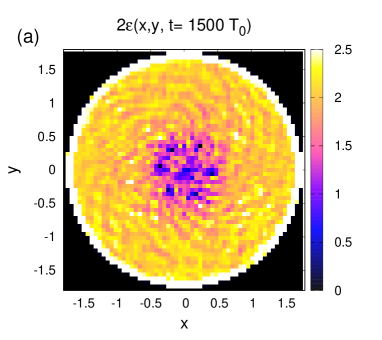
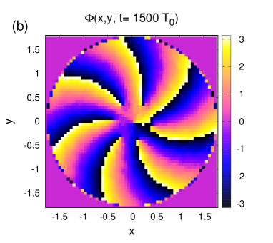
Figure 2: Maps of (a) the doubled energy of oscillators on the lattice and (b) the phase for the rotating cluster of seven vortices on the disk.

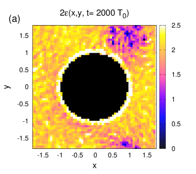
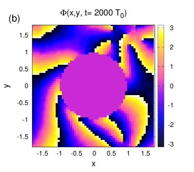
Figure 3: Maps of the (a) doubled energy and (b) phase for the rotating cluster of seven vortices on the torus with the hole.

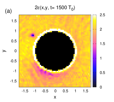
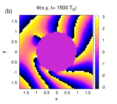
Figure 4: Maps of the (a) doubled energy and (b) phase for the last remaining vortex on the Klein bottle with the hole.

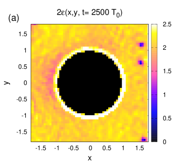
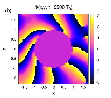
Figure 5: Maps of the (a) doubled energy and (b) phase for three vortices on the projective plane with the hole that move along the perimeter of the square. Finally, only one vortex remains.

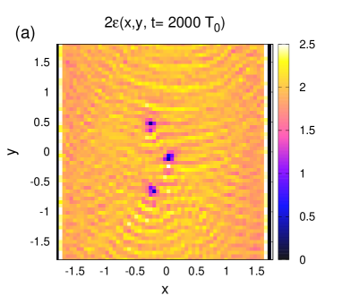
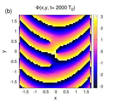
Figure 6: Maps of the (a) doubled energy and (b) phase for vortices on the Möbius strip that move in parallel to the boundary.

III Numerical experiments

In the computer calculations, an element of a two-dimensional array $N_{1}\times N_{2}$ is specified by the multiindex $n=n_{2}+N_{2}n_{1}$, where $0\leq n_{1}\leq N_{1}-1$ and $0\leq n_{2}\leq N_{2}-1$. Only couplings between nearest neighbors or between elements on the opposite sides of the rectangle can be nonzero. If both pairs of the opposite sides are joined by couplings in the direct order [$(0,n_{2})\leftrightarrow(N_{1}-1,n_{2})$, $(n_{1},0)\leftrightarrow(n_{1},N_{2}-1)$], the resulting manifold is a torus. If one pair of the opposite sides are joined in the direct order and the second pair are joined in the reverse order [$(n_{1},0)\leftrightarrow(N_{1}-1-n_{1},N_{2}-1)$], the resulting manifold is a Klein bottle (on this non-orientable manifold, the transition of a vortex through the edge along the “reversed” direction results in its appearance with the opposite sign near the opposite side of the rectangle at the point symmetric with respect to the center). If both pairs of opposite sides are joined in the reverse order, the resulting manifold is a projective plane. Furthermore, if the first pair of opposite sides are not joined altogether, whereas the second pair of opposite sides are joined in the reverse order, the resulting manifold is a Möbius strip. Vortices on the disk were also simulated.

In the numerical experiments reported below, $N_{1}=N_{2}=60$, and, for convenience, sites were located on the square lattice with an arbitrarily chosen step of $h=0.06$ for the total size of the system to be about unity. The external signal ${\cal E}_{n}(t)$ was taken to be monochromatic with the frequency $(1-\Delta)$ for the system to be in the state of nonlinear resonance, where the amplitude of oscillations is determined primarily by the frequency of pumping according to the estimate $gS\approx-\Delta$ and, to a smaller extent, by the amplitude of pumping. For the disk and Möbius strip, the pumping was applied to sites located along the natural boundary. A disk was cut from the torus, Klein bottle, and projective plane, and the signal was applied on sites near the formed boundary. For the formation of vortices to be energetically favorable, the initial phases of the signal depended on $n$, uniformly increasing at bypass along the boundary to the value $2\pi M$, where $M$ is an integer about 10. In the case of the disk and torus, the number $M$ determined the number of vortices in the formed cluster (at the sufficient amplitude of force). In all other cases, no simple correspondence existed between $M$ and the number of vortices: they appeared and disappeared both in the form of vortex-antivortex pairs and singly at collisions with the circular boundary.

Because of a large number of parameters involved in numerical experiments, the results obtained are still insufficient for the complete description of all possible dynamic regimes. For this reason, only some examples are given. However, even these examples clearly demonstrate nontrivial properties of vortices on electric circuits. The parameters were as follows: $R_{L}=0.001$, $1/R_{C}=0.0001$, $C_{n,n^{\prime}}=0.1$, $1/(R_{n,n^{\prime}}C_{n,n^{\prime}})=0.0001$, the amplitude of the external signal was $0.06$, detuning of its frequency $\Delta=0.14$, and $M=7$. All oscillators in the initial state had $I_{n}(0)=0$ and the same values $V_{n}(0)\sim 1$. After an initial transient period continuing about $1000T_{0}$, a quite uniform background density was established on which nucleated vortices moved. Their further evolution significantly depended on the topology of the manifold, as seen in Figs.2-6, which show maps of the energies of oscillators $\varepsilon_{n}$ on the lattice, as well as the quantities $\Phi_{n}=\arctan(I_{n}/V_{n})$, which are qualitatively similar to canonical phases $\Theta_{n}$. In particular, a vortex cluster was formed on the disk, as seen in Fig.2. Vortices in this cluster rotated slowly and changed their mutual arrangement. A similar quiescent regime of rotation of the cluster also occurred in the case of the torus shown in Fig.3. The dynamics on the Klein bottle and projective plane occurred differently, where compact clusters were not formed and the number of vortices decreased gradually with the time (see Figs. 4 and 5, where the difference between the boundary conditions is due to the direct or reverse order of joining of opposite sides and becomes obvious from the comparison of maps of the “phase” $\Phi$). The last remaining vortex on the Klein bottle “was trapped” near the edge of the hole. The last vortex on the projective plane moved along the perimeter of the square clockwise. Vortices on the Möbius strip moved in parallel to the boundary, rarely annihilating pairwise at collisions. In this case, three vortices shown in Fig.6 still remained at times to $5000T_{0}$.

Calculations were also performed with other sets of parameters, e.g., with increased or decreased active resistances, with different frequencies and amplitudes of pumping, as well as with nonuniform profiles of couplings (different $C_{n,n^{\prime}}$ values in different parts of a manifold). Generally speaking, the dynamics of vortices was sometimes strongly different from that described above. In some cases, dark solitons were observed in addition to vortices. All details cannot be discussed here. Important is the fact that long-lived vortices are not exclusive objects requiring fine adjustment of the system but occur in a wide region of parameters.

IV Conclusions

To summarize, a new example of a dynamic system describing modulationally stable nonlinear waves in a weakly dissipative two-dimensional electric circuit has been presented. The numerical simulation has confirmed a scenario according to which resonance pumping concentrated at the edge of such systems results in the formation of an almost uniform background density against which discrete vortices appear and exist for a long time. Such vortices on topologically complex manifolds have been numerically demonstrated for the first time. The derivation (in spatially continuous limit) of equations of motion directly for coordinates of “point” vortices in the presence of dissipation and pump is a problem for the future. Such equations will apparently be more complex than those for the case of free relaxation considered in [29,45].

This work was motivated in particular by interest in the development of artificial materials (including three-dimensional) that can support macroscopic quantum vortices without the Planck constant at room temperature. It is clear that such a material consisting of many millions of units cannot be constructed from radio engineering elements. Its elements should be simpler and cheaper. However, I hope that the general idea of this work will be practically useful for further studies in this field.

References

- (1) L. M. Pismen, Vortices in Nonlinear Fields (Clarendon, Oxford, 1999).
- (2) C. J. Pethick and H. Smith, Bose-Einstein Condensation in Dilute Gases, (Cambridge University Press, Cambridge, 2002).
- (3) L. P. Pitaevskii and S. Stringari, Bose-Einstein Condensation (Oxford University Press, Oxford, 2003).
- (4) P. G. Kevrekidis, D. J. Frantzeskakis, and R. Carretero-González, The Defocusing Nonlinear Schrödinger Equation: From Dark Solitons and Vortices to Vortex Rings (SIAM, Philadelphia, 2015).
- (5) B. Y. Rubinstein and L. M. Pismen, Physica D 78, 1 (1994).
- (6) A. A. Svidzinsky and A. L. Fetter, Phys. Rev. A 62, 063617 (2000).
- (7) A. L. Fetter, Rev. Mod. Phys. 81, 647 (2009).
- (8) V. P. Ruban, Phys. Rev. E 64, 036305 (2001).
- (9) J. Garcia-Ripoll and V. Perez-Garcia, Phys. Rev. A 64, 053611 (2001).
- (10) J. R. Anglin, Phys. Rev. A 65, 063611 (2002).
- (11) P. Rosenbusch, V. Bretin, and J. Dalibard, Phys. Rev. Lett. 89, 200403 (2002).
- (12) A. Aftalion and I. Danaila, Phys. Rev. A 68, 023603 (2003).
- (13) T.-L. Horng, S.-C. Gou, and T.-C. Lin, Phys. Rev. A 74, 041603(R) (2006).
- (14) V. A. Mironov and L. A. Smirnov, JETP Lett. 95, 549 (2012).
- (15) S. Serafini, M. Barbiero, M. Debortoli, S. Donadello, F. Larcher, F. Dalfovo, G. Lamporesi, and G. Ferrari, Phys. Rev. Lett. 115, 170402 (2015).
- (16) S. Serafini, L. Galantucci, E. Iseni, T. Bienaime, R. N. Bisset, C. F. Barenghi, F. Dalfovo, G. Lamporesi, and G. Ferrari, Phys. Rev. X 7, 021031 (2017).
- (17) C. Ticknor, W. Wang, and P. G. Kevrekidis, Phys. Rev. A 98, 033609 (2018).
- (18) V. P. Ruban, JETP Lett. 108, 605 (2018).
- (19) C. Ticknor, V. P. Ruban, and P. G. Kevrekidis, Phys. Rev. A 99, 063604 (2019).
- (20) B. A. Malomed and P. G. Kevrekidis, Phys. Rev. E 64, 026601 (2001).
- (21) P. G. Kevrekidis, B. A. Malomed, and Yu. B. Gaididei, Phys. Rev. E 66, 016609 (2002).
- (22) P. G. Kevrekidis, B. A. Malomed, D. J. Frantzeskakis, and R. Carretero-Gonzalez, Phys. Rev. Lett. 93, 080403 (2004).
- (23) P. G. Kevrekidis, B. A. Malomed, Zh. Chen, and D. J. Frantzeskakis, Phys. Rev. E 70, 056612 (2004).
- (24) D. E. Pelinovsky, P. G. Kevrekidis, and D. J. Frantzeskakis, Physica D 212, 20 (2005).
- (25) F. Lederer, G. I. Stegeman, D. N. Christodoulides, G. Assanto, M. Segev, and Ya. Silberberg, Phys. Rep. 463, 1 (2008).
- (26) J. Cuevas, G. James, P. G. Kevrekidis, and K. J. H. Law, Physica D 238, 1422 (2009).
- (27) Ya. V. Kartashov, B. A. Malomed, and L. Torner, Rev. Mod. Phys. 83, 247 (2011).
- (28) M. Lapine, I. V. Shadrivov, and Yu. S. Kivshar, Rev. Mod. Phys. 86, 1093 (2014).
- (29) V. P. Ruban, Phys. Rev. E 100, 012205 (2019).
- (30) N. N. Rosanov, N. V. Vysotina, A. N. Shatsev, I. V. Shadrivov, and Yu. S. Kivshar’, JETP Lett. 93, 743 (2011).
- (31) R. Hirota and K. Suzuki, J. Phys. Soc. Jpn. 28, 1366 (1970).
- (32) R. Hirota and K. Suzuki, Proc. IEEE 61, 1483 (1973).
- (33) A. C. Hicks, A. K. Common, and M. I. Sobhy, Physica D 95, 167 (1996).
- (34) A. C. Singer and A. V. Oppenheim, Int. J. Bifurcation Chaos 9, 571 (1999).
- (35) D. Cai, N. Gronbech-Jensen, A.R. Bishop, A.T. Findikoglu, and D. Reagor, Physica D 123, 291 (1998).
- (36) T. Kofane, B. Michaux, and M. Remoissenet, J. Phys. C: Solid State Phys. 21, 1395 (1988).
- (37) P. Marquie, J. M. Bilbault, and M. Remoissenet, Phys. Rev. E 49, 828 (1994).
- (38) P. Marquie, J. M. Bilbault, and M. Remoissenet, Phys. Rev. E 51, 6127 (1995).
- (39) V. A. Makarov, E. del Rio, W. Ebeling, and M. G. Velarde, Phys. Rev. E 64, 036601 (2001).
- (40) D. Yemele, P. Marquie, and J. M. Bilbault, Phys. Rev. E 68, 016605 (2003).
- (41) L. Q. English, F. Palmero, A. J. Sievers, P. G. Kevrekidis, and D. H. Barnak, Phys. Rev. E 81, 046605 (2010).
- (42) F. Palmero, L. Q. English, J. Cuevas, R. Carretero-Gonzalez, and P. G. Kevrekidis, Phys. Rev. E 84, 026605 (2011).
- (43) L. Q. English, F. Palmero, J. F. Stormes, J. Cuevas, R. Carretero-Gonzalez, and P. G. Kevrekidis, Phys. Rev. E 88, 022912 (2013).
- (44) F. Palmero, L. Q. English, X.-L. Chen, W. Li, J. Cuevas-Maraver, and P. G. Kevrekidis, Phys. Rev. E 99, 032206 (2019).
- (45) V. P. Ruban, arXiv:1910.07827
- (46) C. J. G. Meyers, C. R. Freeze, S. Stemmer, and R. A. York, Appl. Phys. Lett. 109, 112902 (2016).
- (47) Y. Shen, P. G. Kevrekidis, G. P. Veldes, D. J. Frantzeskakis, D. DiMarzio, X. Lan, and V. Radisic, Phys. Rev. E 95, 032223 (2017).
- (48) F. J. Munoz, S. K. Turitsyn, Yu. S. Kivshar, and M. I. Molina, Phys. Rev. A 95, 033833 (2017).
- (49) A. P. Slobozhanyuk, P. V. Kapitanova, I. V. Shadrivov, P. A. Belov, and Yu. S. Kivshar’, JETP Lett. 95, 613 (2012).