Coverage Analysis of UAVs in Millimeter Wave Networks: A Stochastic Geometry Approach

Abstract

Recent developments in robotics and communication technologies are paving the way towards the use of Unmanned Aerial Vehicles (UAVs) to provide ubiquitous connectivity in public safety scenarios or in remote areas. The millimeter wave (mmWave) spectrum, in particular, has gained momentum since the huge amount of free spectrum available at such frequencies can yield very high data rates. In the UAV context, however, mmWave operations may incur severe signal attenuation and sensitivity to blockage, especially considering the very long transmission distances involved. In this paper, we present a tractable stochastic analysis to characterize the coverage probability of UAV stations operating at mmWaves. We exemplify some of the trade-offs to be considered when designing solutions for millimeter wave (mmWave) scenarios, such as the beamforming configuration, and the UAV altitude and deployment.

I Introduction

In recent years the usage of Unmanned Aerial Vehicles (UAVs), commonly known as drones, has rapidly grown thanks to the extremely low operating and maintenance costs, and to the ease of deployment. When equipped with dedicated sensors, UAVs can support several services, from airspace surveillance and border patrol [1] to traffic and crowd monitoring [2]. Recently, drones have been studied as a solution to provide coverage and connectivity to ground users and first responders in emergency situations [3], e.g., when cellular infrastructures are either unavailable or no longer operational [4]. UAVs can also be deployed on-demand, to boost base station’s capacity in hot-spot areas or when terrestrial infrastructures are overloaded [5].

Today, UAV communications are typically enabled by legacy wireless technologies such as Long Term Evolution (LTE) [6] or Wi-Fi which, however, cannot satisfy the very strict reliability, throughput and latency requirements of future applications [7]. In these regards, 5th generation (5G) innovations, especially network operations in the millimeter wave (mmWave) spectrum, may offer a practical solution to overcome existing cellular connectivity shortfalls [8]. In fact, the large spectrum available at mmWaves, in combination with massive Multiple Input Multiple Output (MIMO) technologies, makes it possible to achieve multi-Gbps transmission speeds, as well as to guarantee spatial isolation and immunity to jamming and eavesdropping through directional communication [9].

Nevertheless, the application of mmWave solutions to UAV networks is hindered by the severe signal power attenuation experienced at high frequency. As a matter of fact, mmWave propagation suffers from adverse environmental conditions (principally rain, but also foliage and atmospheric attenuation), human and self blockage, shadowing, and high material penetration loss [10]. Furthermore, unlike on-the-ground devices, UAVs are fast-moving, and hence create Doppler. Additionally, the establishment of directional transmissions requires periodic beam tracking to maintain alignment, an operations that may increase the communication latency, especially in high velocity flight, and result in Quality of Service (QoS) degradation [11]. Moreover, UAV operations are further complicated by high propulsion energy consumption to maintain and support their movements, thereby posing severe power management constraints [12]. These limitations pose new challenges for proper protocol design and exemplify how UAV connectivity performance in the mmWave scenario is heavily influenced by the specific characteristics of the environment in which the nodes are deployed.

In light of the above challenges, in this paper we apply stochastic geometry to evaluate the practical feasibility of deploying UAV-based networks operating at mmWaves. To the best of our knowledge, this is the first contribution that provides an analytical expression for the UAV coverage probability for mmWave scenarios, i.e., the probability that a reference ground User Equipment (UE) experiences a link quality (which is measured in terms of Signal to Noise Ratio (SNR)) above a certain threshold. Our analysis investigates the impact of several UAV-specific parameters on the overall network performance, including the UAV density, altitude, and antenna configuration. We validate our theoretical model through Monte Carlo simulations and demonstrate that, while a lower altitude is typically correlated with lower signal power attenuation, it also results in more likely non-line-of-sight links due to buildings and other obstacles in the environments, thus leading to intermittent connectivity. Moreover, we show that a peak in the coverage probability can be associated with an optimal deployment altitude, above which the coverage probability degrades due to the increased UAV-UE distance, and characterize the configurations of the network that minimize the number of deployed UAVs without compromising the coverage.

The rest of this paper is organized as follows. In Sec. II we overview the most recent works on UAV networks, in Sec. III we present our stochastic model for evaluating the coverage probability in a general UAV scenario, in Sec. IV we present numerical results and validate our theoretical framework, and in Sec. V we conclude our work with suggestions for future research.

II Related Work

Given the recent advances in UAV design and deployment, the research community is studying how cellular and ad hoc networks can benefit from the integration between wireless communications and flying platforms [13]. The 3rd Generation Partnership Project (3GPP) has examined several study items for the support of UAV-mounted UEs in LTE [14], and will consider more advanced solutions for NR, with the possibility of deploying base stations on UAVs themselves [15].

The interest in UAV communications has led to several studies on channel modeling [16, 17], performance evaluation [18], and mobility management [19] in flying networks. Additionally, the combination of UAVs and mmWaves is seen as a promising enabler of multi-Gbps networks that can be instantiated on the fly [20], to serve, for example, public safety scenarios [21]. A review of the challenges and opportunities for the integration of mmWaves and UAVs can be found in [22]. MmWaves can also be used to establish backhaul links in UAV deployments [23]. Two challenges that still have to be solved in the domain of UAVs and mmWaves are channel modeling (some early results have been presented in [24, 25]) and beam management, which is made more challenging by the high mobility of the flying platform [26].

Stochastic geometry has been widely used to characterize the behavior of UAV networks. In [27, 28] the authors derived the UAV coverage distribution for a network under guaranteed LOS conditions, considering Nakagami-m small-scale fading. The authors of [29] model UAV base stations with a Poission Point Process (PPP), varying the height to maximize the coverage probability. Similarly, the authors of [30] try to optimize the UAV density, assuming LOS links, while in [31] a stochastic model jointly optimizes density, height and antenna patterns. Liu et al., in [32], computed the lower and upper bounds of the coverage probability and area spectral efficiency of UAV networks, assuming, respectively, that UAVs are hovering randomly according to a homogeneous PPP, or that they can instantaneously move to the positions directly above the intended ground users.

In [33], the authors analyze the wireless backhaul links of a UAV network operating in an urban environment in the presence of LOS-blocking buildings, assuming independent distributions of the transmitters and receivers. With respect to the possible applications, [34] evaluates the performance of a UAV swarm acting alongside a terrestrial network in an emergency outage scenario, and [35] models the coverage for capacity in hot-spot scenarios. In [36], a communication network with an underlay aerial base station is deployed to provide coverage for a temporary event (such as a concert in a stadium or a sporting event). Interestingly, the model divides the space allocated to the temporary event, modeled by a disk of radius $R_{2}$, and the UAV, deployed at a certain height $h$ at the center of the disk.

While these papers provide solid models and optimizations for UAV wireless networks, they focus on propagation at sub-6 GHz frequencies. The literature currently lacks works combining stochastic geometry models, UAV networks and the mmWave band. In this paper we fill this gap by deriving the coverage probability for a stochastic UAV network operating at mmWaves, depending on communication and deployment choices (e.g., beamforming design, deployment height and density).

III Stochastic Coverage Analysis

In this section we analyze the coverage of the UAV scenario based on a stochastic analysis. In detail, in Sec. III-A we describe our system model, in Sec. III-B we present the association rule for the UE and derive a probabilistic expression for the distance between the UE and its serving UAV, while in Sec. III-C we provide the expression for the coverage probability.

III-A System Model

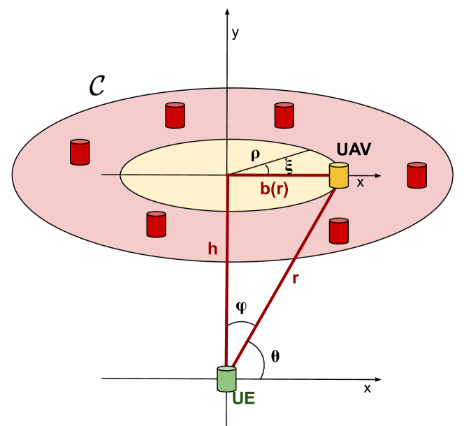
Fig. 1: UAV system model. The reference ground UE is represented at the origin of a Cartesian system $\{x,y\}$ (green box) and at distance $r$ from the target UAV (yellow box). All other UAVs (red boxes) are deployed in a circular area according to a PPP $\Phi_{\rm UAV}$.

Network model. Fig. 1 provides a graphical representation of the scenario of our analysis. Without loss of generality, we assume that a reference ground UE is placed at the origin of a Cartesian system $\{x,y\}$ centered at point $O=(0,0)$. We also assume that UAVs are deployed across a circular Area of Interest (AoI) $\mathcal{C}$ at an altitude $h$ to form a 2D homogeneous PPP $\Phi_{\rm UAV}$ of intensity measure $\lambda_{\rm UAV}$. We must mention that, even though the network should be modeled in the 3D Euclidean space, for the tractability of the analysis, our approach deploys UAVs at the same altitude $h$ so that the overall 3D system could be seen as a superposition of a first ground plane $\Pi^{{}^{\prime}}=\{x^{{}^{\prime}},y^{{}^{\prime}}\}\subseteq\mathbb{R}^{2}$ (with the reference ground UE at position $O$) and a second plane $\Pi^{{}^{\prime\prime}}=\{x^{{}^{\prime\prime}},y^{{}^{\prime\prime}}\}\subseteq\mathbb{R}^{2}$ which includes the AoI $\mathcal{C}\subseteq\mathbb{R}^{2}$. We then call $r$ the 2D distance between the reference ground UE and a generic UAV in the AoI at altitude $h$, and $b(r)=\sqrt{r^{2}-h^{2}}$ the distance between the projection of the UE on $\Pi^{{}^{\prime\prime}}$ and the generic UAV.

Path loss model. In the UAV scenario, especially at low elevation angles, we expect that environmental objects (e.g., buildings, vegetation) will act as obstacles to the propagation of the signals. It is thus imperative to distinguish between Line of Sight (LOS) and Non Line of Sight (NLOS) propagation (denoted with subscripts $L$ and $N$, respectively, throughout the paper). In particular, UAV $n$ is assumed to be in LOS (with probability $p_{L}(r)$) if the segment connecting the reference ground UE and UAV $n$ (at distance $r$) does not intersect any blockage. In this paper, $p_{L}(r)$ is modeled as in [16] as a function of the elevation angle $\theta=\arcsin(h/r)$, i.e.,

$$p_{L}(r)=\frac{1}{1+C\exp\left[-Y\left(\arcsin\left(\frac{h}{r}\right)\frac{180}{\pi}-C\right)\right]},$$ (1)

where $C$ and $Y$ are environment-related parameters whose values will be detailed in Sec. IV. Similarly, UAVs are assumed to be in NLOS with complementary probability $p_{N}(r)=1-p_{L}(r)$.

By the thinning theorem of PPP [37], we can distinguish two independent PPPs for the LOS and NLOS UAVs, i.e., $\Phi_{\text{UAV},L}\subseteq\Phi_{\rm UAV}$ and $\Phi_{\text{UAV},N}\subseteq\Phi_{\rm UAV}$ respectively, of intensity measure $\lambda_{\text{UAV},L}=p_{L}(r)\lambda_{\rm UAV}$, and $\lambda_{\text{UAV},N}=p_{N}(r)\lambda_{\rm UAV}$ respectively. Consequently, the path gain $\ell_{i}(r)$ between the reference ground UE and the generic UAV $\in\Phi_{\text{UAV},i}$, $i\in\{L,N\}$, at distance $r$, is expressed as

$$\ell_{i}(r)=C_{i}r^{-a_{i}}$$ (2)

where $a_{i}$ is the path loss exponent and $C_{i}$ is the path loss gain at unit distance.

Antenna model. As introduced in Sec. I, mmWave communication requires large antenna arrays to be installed at both the UAVs and the UEs to benefit from the resulting antenna gain and overcome the severe path loss experienced at high frequency. In this paper, the UAV (UE) antenna array is modeled as a Uniform Planar Array (UPA) of $\mathcal{N}_{\rm UAV}$ ($\mathcal{N}_{\rm UE}$) elements. For the tractability of the analysis and consistently with related work on stochastic geometry (e.g., [38, 39]), we assume that antenna patterns are approximated by a sectored antenna model, and we call $G=\mathcal{N}_{\rm UAV}\times\mathcal{N}_{\rm UE}$ the overall antenna gain (assumed constant for all angles in the main lobe) in case of perfect beam alignment between the reference ground UE and its serving UAV.

Channel model. In order to describe correctly the UAV channel profile at mmWaves, small-scale fading is modeled via a Nakagami distribution which is generic enough to incorporate both LOS and NLOS air-to-ground channels [40] and has been demonstrated to accurately characterize mmWave propagation (e.g., reflectivity and scattering from common objects), especially when directional beamforming is applied [41].

III-B Association Rule

Let $r_{n}$ be the distance between the reference ground UE and the UAV $n$. We assume that the UE always connects to the UAV $n^{*}\in\Phi_{\text{UAV},i}$, $i\in\{L,N\}$ that provides the maximum path gain, meaning the UAV whose attributes produce the minimum path loss to the signal, i.e.,

$$n^{*}=\operatorname*{arg\,max}_{\forall i\in\{L,N\},\forall n\in\Phi_{i}}{\ell_{i}(r_{n})},$$ (3)

where ${\ell_{i}(r_{n})}$ is given in Eq. (2).

Based on the above definition, we can evaluate the Probability Density Function (PDF) of the distance between the reference ground UE and the closest available LOS or NLOS UAV (which does not necessarily imply a direct correspondence with the UAV that will be selected for association).

       Lemma 1:

The probability density function of the distance $r$ between the reference ground UE and the closest UAV of type $i=\{L,N\}$ is

$$f_{i}(r) =2\pi\lambda_{\rm UAV}rp_{i}(b(r))\exp\left(-2\pi\lambda_{\rm UAV}\int_{0}^{b(r)}p_{i}(\rho)\rho d\rho\right)$$ (4)

where $b(r)=\sqrt{r^{2}-h^{2}}$, $p_{i}\Big{(}b(r)\Big{)}$ is the UAV path loss probability as given in Eq. (1) evaluated at horizontal distance $b(r)$ and $i\in\{L,N\}$ depending on the UAV path loss state.

Proof: See Appendix A. $\blacksquare$

Another important factor to be taken into account is the possibility of associating not to the closest UAV (distance-wise) but to the one offering the best communication performance, as per the association rule defined previously, especially when considering a very dense urban environment in which the nearest available UAV may be NLOS [39]. Therefore we can model the probability $P_{i}$ of connecting to a UAV of type $i=\{L,N\}$ as the probability that the distance $r_{i^{*}}$ between the reference ground UE and the closest UAV of opposite type $i^{*}=\{N,L\}$ is greater than or equal to $A_{i}(r)$, defined as

$$A_{i}(r)=\left(\frac{C_{i^{\ast}}}{C_{i}}r^{a_{i}}\right)^{\frac{1}{a_{i}^{*}}},$$ (5)

where $i^{*}$ represents the path loss state opposite to $i$. As a result, assuming that the reference UE connects to a LOS (NLOS) UAV, the problem can be reformulated by modeling the probability that there are no NLOS (LOS) UAVs inside a circular area of radius $b(A_{L}(r))$ ($b(A_{N}(r))$). The related probability $P_{i}$ is then expressed as in the following lemma.

       Lemma 2:

The probability $P_{i}$ of connecting to a UAV $\in\Phi_{\text{UAV},i}$, with $i=\{L,N\}$, is

$$P_{i}=\int_{h}^{\infty}\exp\left(-2\pi\lambda_{\rm UAV}\int_{0}^{b(A_{i}(r))}p_{i^{\ast}}(\rho)\rho d\rho\right)f_{i}(r)dr,$$ (6)

with $b(A_{i}(r))=\sqrt{A_{i}(r)^{2}-h^{2}}$ being the horizontal distance in the plane $\Pi^{\prime\prime}\subseteq\mathbb{R}^{2}$ to the UAV at distance $A_{i}(r)$ from the reference ground UE.

Proof: See Appendix B. $\blacksquare$

As a final step, we can derive the expression of the PDF of the association distance with a UAV of type $i=\{L,N\}$ in the following lemma.

       Lemma 3:

The probability density function $\overline{f}_{i}(r)$ of the association distance to a UAV $\in\Phi_{\text{UAV},i}$, with $i\in\{L,N\}$ at distance $r$ from a reference ground UE is expressed as

$$\overline{f}_{i}(r)=\exp\left(-2\pi\lambda_{UAV}\int_{0}^{b(A_{i}(r))}p_{i^{\ast}}(\rho))\rho d\rho\right)f_{i}(r).$$ (7)

Proof: The proof follows the same line of reasoning from Lemma 2 and is omitted here. $\blacksquare$

III-C Coverage Probability

In this subsection we provide an analytical closed-form expression for the coverage probability $P_{\rm cov}(\Gamma)$ of a reference ground UE, i.e., the probability that the reference user experiences an SNR larger than a target threshold $\Gamma$ (usually in the order of a few dB). Analytically, $P_{\rm cov}(\Gamma)=\mathbb{P}[\text{SNR}(r)>\Gamma]$, where the SNR experienced by the UE, attached to a UAV $\in\Phi_{\rm UAV},i$, with $i\in\{L,N\}$, at distance $r$ is given as

$$\text{SNR}_{i}=\frac{P_{\rm TX}\ell_{i}(r)Gg}{\text{NF}\cdot\sigma^{2}}.$$ (8)

In Eq. (8), $P_{\rm TX}$ is the transmit power, $\ell_{i}(r)$ is the path gain profile as expressed in Eq. (2), $G=\mathcal{N}_{\rm UAV}\times\mathcal{N}_{\rm UE}$ is the aggregate beamforming gain, $g$ is the small-scale fading, NF is the noise figure and $\sigma^{2}$ is the power of the thermal noise.

By the law of total probability, we can split the SNR contribution due to the presence of LOS and NLOS conditions for the channel, so the coverage probability becomes

$$P_{\rm cov}(\Gamma)=\mathbb{P}\Big{[}\text{SNR}>\Gamma\Big{]}$$

$$=\mathbb{P}\Big{[}\text{SNR}_{L}>\Gamma,n^{*}\in\Phi_{L}\Big{]}+\mathbb{P}\Big{[}\text{SNR}_{N}>\Gamma,n^{*}\in\Phi_{N}\Big{]},$$ (9)

where $n^{*}$ is the serving UAV according to the association rule defined in Sec. III-B. Based on the lemmas and assumptions of the previous sections, we can formalize the SNR coverage probability in the following theorem.

       Theorem 1:

The coverage probability $P_{\rm cov}(\Gamma)$ for an SNR threshold $\Gamma$, considering a Nakagami$(m_{i},\Omega_{i})$ distributed fading $g$ of shape $m_{i}$ and spread $\Omega_{i}$, with $i\in\{L,N\}$, is given by

$$P_{\rm cov}(\Gamma) =\sum_{i\in\{L,N\}}\int_{h}^{\infty}\left(1-\frac{\int_{0}^{\Delta_{i}}t^{m_{i}-1}e^{-t}dt}{\left(m_{i}-1\right)!}\right)\overline{f}_{i}(r)dr,$$ (10)

where $\Delta_{i}=\frac{m_{i}}{\Omega_{i}}\zeta_{i}(r)^{2}$ and $\zeta_{i}(r)=\frac{\Gamma\left(\text{NF}\cdot\sigma^{2}\right)}{P_{\rm TX}GC_{i}}r^{a_{i}}$.

Proof: See Appendix C. $\blacksquare$

IV Performance Evaluation

This section reports a numerical evaluation of the coverage for UAVs in mmWave scenarios. The results are based on the analytical model introduced in Sec. III, and on a Monte Carlo simulation campaign that we run to validate our analysis.

IV-A Scenario

We deploy UAVs operating at $f_{c}=28$ GHz. For the channel model, we consider the parameters reported in Table I: the LOS probability for UAVs follows Eq. (1), the path gain is modeled according to [42], which considers measurements in a typical urban context (i.e., New York City), while the fading is modeled with a Nakagami random variable with parameters from [40].

Table II summarizes the configuration parameters for the network. Notably, in the following, we will evaluate the coverage by varying (i) the number of antenna elements $\mathcal{N}_{\rm UAV}$ and $\mathcal{N}_{\rm UE}$ in the arrays of the UAVs and UEs, respectively; (ii) the SNR threshold $\Gamma$, which discriminates a link with a high enough quality or not; (iii) the altitude $h$ at which the UAVs are deployed; and (iv) the density $\lambda_{\rm UAV}$ in terms of UAV/km².

For the Monte Carlo simulation, we generated $1000$ random realizations of a PPP in an AoI of radius $2000$ m, for each configuration of parameters. In the following figures, the markers indicate the Monte Carlo simulation results, while the lines represent the numerical results for the analytical model, solved using the MATLAB Symbolic toolbox.

TABLE I: Parameters of the channel model, from [42, 40, 16].

Parameter	LOS Value	NLOS Value
Nakagami-m shape parameter	$m_{L}=3$	$m_{N}=2$
Nakagami-m spread parameter	$\Omega_{L}=1$	$\Omega_{N}=1$
Path gain intercept	$C_{L}=10^{-6.14}$	$C_{N}=10^{-7.2}$
Path gain exponent	$a_{L}=2$	$a_{N}=2.92$
Urban LOS probability parameters	$C=9.6117$	$Y=0.1581$

TABLE II: Parameters of the communication scenario

Parameter	Value
Transmit power $P_{\rm TX}$	20 dBm
Antenna configurations ($\mathcal{N}_{\rm UAV}\times\mathcal{N}_{\rm UE}$)	$[8\times 4]$, $[8\times 8]$, $[64\times 4]$
	$[256\times 4]$, $[256\times 8]$
Noise figure NF	5 dB
Thermal noise $\sigma^{2}$	-84 dBm
SNR threshold $\Gamma$	$[-5,0,5]$ dB
UAV deployment height $h$	$[0-1000]$ m
UAV deployment density $\lambda_{\rm UAV}$	$[1,5,10,15,25]$ UAVs/km2

(a) $\Gamma=-5$ dB

(b) $\Gamma=0$ dB

(c) $\Gamma=5$ dB

Fig. 2: Coverage probability $P_{\rm cov}$ vs. the deployment height $h$ and the SNR threshold $\Gamma$. The antenna configuration has $\mathcal{N}_{\rm UAV}=8$ and $\mathcal{N}_{\rm UE}=8$. The lines represent the numerical results given by the analytical model, and the markers the Monte Carlo simulations.

IV-B Impact of the SNR threshold

Fig. 3: Coverage probability as a function of the UAV density $\lambda_{\rm UAV}$, for different configurations of the antenna arrays at the UAVs ($\mathcal{N}_{\rm UAV}$) and UEs ($\mathcal{N}_{\rm UE}$) , with $\Gamma=5$ dB and a fixed height $h=200$ m.

Fig. 2 reports the trend of $P_{\rm cov}$ for different values of the SNR threshold $\Gamma$, the UAV height $h$ and the UAV deployment density $\lambda_{\rm UAV}$. The coverage probability exhibits a bell shape, with a peak at a specific value of the altitude $h_{\rm opt}$, which is given by the combination of two factors. On one hand, if the UAVs are deployed at low altitudes, the LOS probability will be small, thus the increased pathloss in NLOS will penalize the probability of having an SNR above the threshold $\Gamma$. Conversely, for high altitudes, even if the link is likely in LOS, the impact of the increased distance between the reference UE and its serving UAV decreases the overall link budget, preventing a successful communication.

Notice that, as we do not model the interference in the coverage probability estimation, the performance of the network monotonically increases when considering larger values of the deployment density $\lambda_{\rm UAV}$. Notably, for $\Gamma=0$ dB, only densities higher than 10 UAVs/km² reach $P_{\rm cov}\simeq 1$ at the optimal height. In general, the deployment with $\lambda_{\rm UAV}=1$ UAVs/km² severely underperforms the others, with a gap of 0.12 (for $\Gamma=-5$ dB), 0.45 (for $\Gamma=0$ dB), and 0.55 (for $\Gamma=5$ dB) in the optimal coverage probability obtained with $\lambda_{\rm UAV}=5$ UAVs/km². With $\Gamma=-5$ or 0 dB, however, it does not make sense to increase the deployment density above 5 UAV/km² and 10 UAV/km², respectively, as $P_{\rm cov}$ saturates to 1 for the peak altitude.

Finally, when increasing $\Gamma$ (i.e., the minimum quality required to establish the link), the coverage probability decreases, as expected. In particular, while for $\Gamma=-5$ dB only the configuration with $\lambda_{\rm UAV}=1$ UAVs/km² does not reach $P_{\rm cov}=1$, with $\Gamma=5$ dB none of the configurations peaks at 1, with $\lambda_{\rm UAV}=25$ UAVs/km² having a maximum value of 0.99. This is reasonable as an increase in the minimum acceptable SNR value for coverage translates into a tighter constraint on the link budget of the communication link. Additionally, it can be seen that, besides a decrease in the maximum value of $P_{\rm cov}$ for increasing values of $\Gamma$, the altitude for which the peak value is reached decreases, showing that the reduction in path gain has a more significant impact on Eq. (10) than the reduction of LOS probability given by lower values of $h$.

IV-C Impact of the Antenna Configuration

The configuration of the antenna array plays a fundamental role in reaching a high coverage probability while maintaining the highest SNR threshold $\Gamma=5$ dB. The beamforming gain, indeed, is fundamental in mmWave communications to compensate for the larger pathloss that is experienced at such high frequencies. Fig. 3 shows the trend of $P_{\rm cov}$ when varying the UAV density $\lambda_{\rm UAV}$ and the number of antenna elements at the transmitter and the receiver. As can be seen, even for small values of $\lambda_{\rm UAV}$ (i.e., 5 UAVs/km²), it is possible to achieve $P_{\rm cov}\geq 0.95$ by using at least 64 antenna elements in the UAV and only 4 in the UEs. Similarly, by comparing the configurations with $\mathcal{N}_{\rm UAV}=8$ (fixed) and with $\mathcal{N}_{\rm UE}$ varying from 4 to 8, it is possible to increase $P_{\rm cov}$ by 2 times for $\lambda_{\rm UAV}$ up to 10 UAVs/km².

IV-D Impact of the Deployment Height

As highlighted in Fig. 2, the height at which the UAVs are deployed is a key configuration parameter of the network. This parameter distinguishes UAV networks from traditional cellular networks, as the latter have constraints on the base station height (e.g., the availability of poles and towers) that are more relaxed when operating UAVs. Fig. 4 reports the values of $P_{\rm cov}$ for different values of $\lambda_{\rm UAV}$ and deployment height $h$. The latter varies between 2 and 202 m, i.e., in a range where the maximum value is smaller than the height at which $P_{\rm cov}$ peaks and then decreases. Fig. 4 shows that, by operating at a higher altitude, it is possible to decrease the deployment density of the UAVs, without compromising the coverage probability. For example, the configurations with $\lambda_{\rm UAV}=1$ UAVs/km², and $h=202$ m, has a similar $P_{\rm cov}$ to that with $h=2$ m and $\lambda_{\rm UAV}=10$ UAVs/km². Notice that, in terms of deployment cost and energy, it is more efficient to operate fewer UAVs, even if placed at a higher altitude. Along this line, given the range of values of $\lambda_{\rm UAV}$ considered in Fig. 4, it is possible to reach the maximum value for $P_{\rm cov}$ only with the highest-altitude deployments.

Fig. 4: Coverage probability as a function of the UAV density $\lambda_{\rm UAV}$, for different values of the altitude of the deployment, $\mathcal{N}_{\rm UAV}=8$ and $\mathcal{N}_{\rm UE}=8$, and $\Gamma=0$ dB.

V Conclusions and Future Work

In this work, we proposed a stochastic geometry framework to characterize the coverage performance of a mmWave UAV network. Our model characterizes the UAVs as two independent LOS and NLOS two-dimensional homogeneous Poisson processes and derives the analytical expression for the SNR coverage probability as a function of the distance between a reference ground user terminal and its serving UAV. We validated our analytical curves with Monte Carlo simulations and investigated the relation between coverage support and UAV altitude, UAV density, antenna architecture and targeted link quality threshold. We demonstrated that there exists an optimal altitude at which the UAV should be placed to satisfy the required signal quality threshold, which depends on the UAV swarm size and beamforming gain.

UAV networks still suffer from several challenges including energy consumption, reduced time of flight and environment-related sensitivity. In particular, future research efforts should be dedicated to discovering the relationship between coverage performance and UAV energy consumption.

Appendix A

The distance from the closest UAV of type $i\in\{L,N\}$ is equal to $r$ if there are no other UAVs of the same type closer than $r$. Taking as a reference the model in Fig. 1, this means that there must be no other UAV of type $i$ in the ball $\mathcal{B}(0,b(r))$, where we can define the positions of the UAVs in $\mathcal{B}(0,b(r))$ in polar coordinates as a function of the variables $\rho$ and $\xi$, with $0\leq\rho\leq b(r)$ and $0\leq\xi\leq 2\pi$. Now, since the process $\Phi_{\text{UAV},i}$ is a 2D homogeneous PPP with intensity measure $\lambda_{\text{UAV},i}$ over $\mathcal{B}(0,b(r))$, we get

$$F_{i}(r) =\mathbb{P}\Big{[}\text{No LOS UAVs in the ball }\mathcal{B}(0,b(r))\Big{]}$$

$$=\exp\left(-\int_{0}^{2\pi}\int_{0}^{b(r)}\lambda_{\text{UAV},i}\rho d\rho d\xi\right)$$

$$\stackrel{{\scriptstyle(a)}}{{=}}\exp\left(-2\pi\lambda_{\rm UAV}\int_{0}^{b(r)}p_{i}(\rho)\rho d\rho\right)$$ (11)

with $b(r)=\sqrt{r^{2}-h^{2}}$ and $(a)$ derives from $\lambda_{\text{UAV},i}=p_{i}(\rho)\lambda_{\rm UAV}$. In Eq. (A), $p_{i}(\rho)$ can be rewritten from (1) as a function of $\rho$ as

$$p_{i}(\rho)=\frac{1}{1+C\exp\left[-Y\left(\arctan\left(\frac{h}{\rho}\right)\frac{180}{\pi}-C\right)\right]}.$$ (12)

The PDF of the distance $r$ to the closest UAV of type $i$ can finally be computed as

$$f_{i}(r)=\frac{\partial}{\partial r}\Big{(}1-F_{i}(r)\Big{)}$$

$$=2\pi\lambda_{\rm UAV}rp_{i}(b(r))\exp\left(-2\pi\lambda_{\rm UAV}\int_{0}^{b(r)}p_{i}(\rho)\rho d\rho\right).$$ (13)

Appendix B

Let $r_{L}$ and $r_{N}$ be random variables expressing the distance of the reference ground UE from the closest LOS and NLOS UAVs, respectively. In order for the user to connect with a LOS (NLOS) UAV, there must be no NLOS (LOS) UAVs at a distance smaller than or equal to $A_{L}(r)$ ($A_{N}(r)$), i.e., the minimum distance at which a potential NLOS (LOS) UAV could provide a better path gain to the user in comparison to its LOS rival. Considering the LOS case, the probability $P_{L}$ of connecting to a LOS UAV can be written as

$$P_{L}(r) =\mathbb{P}\left[C_{L}r_{L}^{-a_{L}}>C_{N}r_{N}^{-a_{N}}\right]$$

$$=\mathbb{P}\left[r_{N}>\left(({C_{N}}/{C_{L}})r^{a_{L}}\right)^{\frac{1}{a_{N}}}\right]$$

$$\stackrel{{\scriptstyle(a)}}{{=}}\int_{h}^{\infty}\mathbb{P}\left[r_{N}>A_{L}(r)\right]f_{L}(r)dr$$ (14)

where $(a)$ follows from the fact that $r>h$ by construction, and $f_{L}$ is the PDF of $r_{L}$ according to Lemma 1. In Eq. (B), $\mathbb{P}\left[r_{N}>A_{L}(r)\right]$ represents the probability that there are no NLOS BS inside the circular area $\mathcal{B}(0,b(A_{L}(r)))$ with radius $b(A_{L}(r))$ and can be computed as

$$\mathbb{P}\left[r_{N}>A_{L}(r)\right]=\exp\left(-2\pi\lambda_{\rm UAV}\int_{0}^{b\left(A_{L}(r)\right)}p_{N}(\rho)\rho d\rho\right),$$ (15)

where $p_{N}(\rho)$ follows from Eq. (12). By substituting (15) into (B), we get the expression in Lemma 2 for the LOS case. With a similar proof, it is possible to prove the lemma also for the NLOS case.

Appendix C

Being $r_{i}$ the distance between the reference ground UE and its serving UAV $n^{*}\in\Phi_{\text{UAV},i}$, with $i\in\{L,N\}$, the probability in Eq. (III-C) can be written as

$$\mathbb{P} \Big{[}\text{SNR}_{i}>\Gamma,n^{*}\in\Phi_{i}\Big{]}=\mathbb{E}_{r_{i}}\Bigg{[}\mathbb{P}\Big{[}\text{SNR}_{i}>\Gamma\Bigl{\lvert}r_{i}\Big{]}\Bigg{]}$$

$$\stackrel{{\scriptstyle(a)}}{{=}}\mathbb{E}_{r_{i}}\Bigg{[}\mathbb{P}\left[\frac{P_{\rm TX}\ell_{i}(r_{i})Gg(m_{i},\Omega_{i})}{\text{NF}\cdot\sigma^{2}}>\Gamma\Bigl{\lvert}r_{i}\right]\Bigg{]}$$

$$=\int_{h}^{\infty}\mathbb{P}\left[g(m_{i},\Omega_{i})>\frac{\Gamma(\text{NF}\cdot\sigma^{2})}{P_{\rm TX}GC_{i}}r^{a_{i}}\Bigl{\lvert}r\right]\overline{f}_{i}(r)dr,$$ (16)

where $(a)$ derives from Eq. (8). Now, with the assumption that the small scale fading $g$ follows a Nakagami distribution of parameters $m_{i}$ and $\Omega_{i}$, $i\in\{L,N\}$, we can derive its associated Cumulative Distribution Function (CDF) as

$$F(x;m_{i},\Omega_{i}) =\mathbb{P}\Big{[}g(m_{i},\Omega_{i})\leq x\Big{]}$$

$$=P\left(m_{i},\frac{m_{i}}{\Omega_{i}}x^{2}\right)=\frac{\gamma(m_{i},\frac{m_{i}}{\Omega_{i}}x^{2})}{\Gamma(m_{i})},$$ (17)

where $P\left(m,\frac{m_{i}}{\Omega_{i}}x^{2}\right)$ is the (regularized) incomplete gamma function, $\gamma(m_{i},\frac{m_{i}}{\Omega_{i}}x^{2})$ is the lower incomplete gamma function and $\Gamma(m_{i})=\left(m_{i}-1\right)!$. Therefore, the probability term inside Eq. (C) becomes

$$\mathbb{P}\left[g(m_{i},\Omega_{i})>\frac{\Gamma(\text{NF}\cdot\sigma^{2})}{P_{\rm TX}GC_{i}}r^{a_{i}}\Bigl{\lvert}r\right]$$

$$=1-P\left(m_{i},\frac{m_{i}}{\Omega_{i}}\zeta_{i}(r)^{2}\right)=1-\frac{\int_{0}^{\Delta_{i}}t^{m_{i}-1}e^{-t}dt}{\left(m_{i}-1\right)!},$$ (18)

where we defined $\zeta_{i}(r)=\frac{\Gamma(\text{NF}\cdot\sigma^{2})}{P_{\rm TX}GC_{i}}r^{a_{i}}$ and $\Delta_{i}=\frac{m_{i}}{\Omega_{i}}\zeta_{i}(r)^{2}$.
By substituting (C) into (C) we get the expression of the coverage probability in Theorem 1.

References

- [1] P. Chandhar, D. Danev, and E. G. Larsson, “Massive MIMO for communications with drone swarms,” IEEE Transactions on Wireless Communications, vol. 17, no. 3, pp. 1604–1629, Mar 2017.
- [2] P. Chandhar and E. G. Larsson, “Massive MIMO for connectivity with drones: Case studies and future directions,” IEEE Access, vol. 7, pp. 94 676–94 691, 2019.
- [3] W. Shi, H. Zhou, J. Li, W. Xu, N. Zhang, and X. Shen, “Drone assisted vehicular networks: Architecture, challenges and opportunities,” IEEE Network, vol. 32, no. 3, pp. 130–137, May/June 2018.
- [4] M. Mezzavilla, M. Polese, A. Zanella, A. Dhananjay, S. Rangan, C. Kessler, T. S. Rappaport, and M. Zorzi, “Public Safety Communications above 6 GHz: Challenges and Opportunities,” IEEE Access, vol. 6, pp. 316–329, 2018.
- [5] M. Giordani and M. Zorzi, “Satellite Communication at Millimeter Waves: a Key Enabler of the 6G Era,” IEEE International Conference on Computing, Networking and Communications (ICNC), Feb 2020.
- [6] B. Van Der Bergh, A. Chiumento, and S. Pollin, “LTE in the sky: Trading off propagation benefits with interference costs for aerial nodes,” IEEE Communications Magazine, vol. 54, no. 5, pp. 44–50, May 2016.
- [7] S. Hayat, E. Yanmaz, and C. Bettstetter, “Experimental analysis of multipoint-to-point UAV communications with IEEE 802.11n and 802.11ac,” in IEEE 26th Annual International Symposium on Personal, Indoor, and Mobile Radio Communications (PIMRC). IEEE, 2015, pp. 1991–1996.
- [8] L. Zhang, H. Zhao, S. Hou, Z. Zhao, H. Xu, X. Wu, Q. Wu, and R. Zhang, “A survey on 5G millimeter wave communications for UAV-assisted wireless networks,” IEEE Access, vol. 7, pp. 117 460–117 504, 2019.
- [9] M. Xiao, S. Mumtaz, Y. Huang, L. Dai, Y. Li, M. Matthaiou, G. K. Karagiannidis, E. Björnson, K. Yang, I. Chih-Lin et al., “Millimeter wave communications for future mobile networks,” IEEE Journal on Selected Areas in Communications, vol. 35, no. 9, pp. 1909–1935, Sept 2017.
- [10] T. S. Rappaport, R. W. Heath Jr, R. C. Daniels, and J. N. Murdock, Millimeter wave wireless communications. Pearson Education, 2014.
- [11] M. Giordani, M. Polese, A. Roy, D. Castor, and M. Zorzi, “A tutorial on beam management for 3GPP NR at mmWave frequencies,” IEEE Communications Surveys & Tutorials, vol. 21, no. 1, pp. 173–196, First quarter 2019.
- [12] C. H. Liu, Z. Chen, J. Tang, J. Xu, and C. Piao, “Energy-efficient UAV control for effective and fair communication coverage: A deep reinforcement learning approach,” IEEE Journal on Selected Areas in Communications, vol. 36, no. 9, pp. 2059–2070, Sept 2018.
- [13] S. Zhang, Y. Zeng, and R. Zhang, “Cellular-enabled UAV communication: A connectivity-constrained trajectory optimization perspective,” IEEE Transactions on Communications, vol. 67, no. 3, pp. 2580–2604, Mar 2019.
- [14] 3GPP, “Study on enhanced LTE support for aerial vehicles,” TR 36.777, V15.0.0, 2017.
- [15] ——, “Unmanned Aerial System (UAS) support in 3GPP,” TR 22.125, V17.1.0, 2019.
- [16] A. Al-Hourani, S. Kandeepan, and S. Lardner, “Optimal LAP altitude for Maximum Coverage,” IEEE Wireless Communications Letters, vol. 3, no. 6, pp. 569–572, Dec 2014.
- [17] N. Ahmed, S. S. Kanhere, and S. Jha, “On the importance of link characterization for aerial wireless sensor networks,” IEEE Communications Magazine, vol. 54, no. 5, pp. 52–57, May 2016.
- [18] M. Mozaffari, W. Saad, M. Bennis, and M. Debbah, “Drone small cells in the clouds: Design, deployment and performance analysis,” in IEEE Global Communications Conference (GLOBECOM). IEEE, 2015.
- [19] L. Bertizzolo, M. Polese, L. Bonati, A. Gosain, M. Zorzi, and T. Melodia, “mmBAC: Location-Aided mmWave Backhaul Management for UAV-Based Aerial Cells,” in 3rd ACM Workshop on Millimeter-Wave Networks and Sensing Systems, ser. mmNets’19. Association for Computing Machinery, 2019.
- [20] T. Cuvelier and R. Heath, “mmWave MU-MIMO for aerial networks,” in Proc. of IEEE ISWCS, Lisbon, Portugal, Aug 2018.
- [21] W. Xia, M. Polese, M. Mezzavilla, G. Loianno, S. Rangan, and M. Zorzi, “Millimeter Wave Remote UAV Control and Communications for Public Safety Scenarios,” in 16th Annual IEEE International Conference on Sensing, Communication, and Networking (SECON), June 2019.
- [22] Z. Xiao, P. Xia, and X. Xia, “Enabling UAV cellular with millimeter-wave communication: Potentials and approaches,” IEEE Communications Magazine, vol. 54, no. 5, pp. 66–73, May 2016.
- [23] M. Gapeyenko, V. Petrov, D. Moltchanov, S. Andreev, N. Himayat, and Y. Koucheryavy, “Flexible and Reliable UAV-Assisted Backhaul Operation in 5G mmWave Cellular Networks,” IEEE Journal on Selected Areas in Communications, vol. 36, no. 11, pp. 2486–2496, Nov 2018.
- [24] W. Khawaja, O. Ozdemir, and I. Guvenc, “UAV air-to-ground channel characterization for mmWave systems,” in Proc. of IEEE VTC-Fall, Toronto, ON, Canada, Sept 2017.
- [25] ——, “Temporal and spatial characteristics of mmWave propagation channels for UAVs,” in Proc. of IEEE GSMM, May 2018.
- [26] J. Zhao, G. Gao, L. Kuang, Q. Wu, and W. Jia, “Channel tracking with flight control system for UAV mmWave MIMO communications,” IEEE Communications Letters, vol. 22, no. 6, pp. 1224–1227, June 2018.
- [27] V. V. C. Ravi and H. S. Dhillon, “Downlink coverage probability in a finite network of unmanned aerial vehicle (UAV) base stations,” in IEEE 17th International Workshop on Signal Processing Advances in Wireless Communications (SPAWC). IEEE, 2016, pp. 1–5.
- [28] V. V. Chetlur and H. S. Dhillon, “Downlink coverage analysis for a finite 3-D wireless network of unmanned aerial vehicles,” IEEE Transactions on Communications, vol. 65, no. 10, pp. 4543–4558, Oct 2017.
- [29] B. Galkin, J. Kibiłda, and L. A. DaSilva, “A stochastic geometry model of backhaul and user coverage in urban UAV networks,” arXiv preprint arXiv:1710.03701, 2017.
- [30] C. Zhang and W. Zhang, “Spectrum sharing for drone networks,” IEEE Journal on Selected Areas in Communications, vol. 35, no. 1, pp. 136–144, Jan 2017.
- [31] M. M. Azari, Y. Murillo, O. Amin, F. Rosas, M.-S. Alouini, and S. Pollin, “Coverage maximization for a poisson field of drone cells,” in IEEE 28th Annual International Symposium on Personal, Indoor, and Mobile Radio Communications (PIMRC). IEEE, 2017.
- [32] C. Liu, M. Ding, C. Ma, Q. Li, Z. Lin, and Y.-C. Liang, “Performance analysis for practical unmanned aerial vehicle networks with LoS/NLoS transmissions,” in IEEE International Conference on Communications Workshops (ICC Workshops). IEEE, 2018, pp. 1–6.
- [33] B. Galkin, J. Kibilda, and L. A. DaSilva, “Backhaul for low-altitude UAVs in urban environments,” in IEEE International Conference on Communications (ICC). IEEE, 2018.
- [34] A. M. Hayajneh, S. A. R. Zaidi, D. C. McLernon, and M. Ghogho, “Drone empowered small cellular disaster recovery networks for resilient smart cities,” in IEEE international conference on sensing, communication and networking (SECON Workshops). IEEE, 2016.
- [35] B. Galkin, J. Kibiłda, and L. A. DaSilva, “A stochastic model for UAV networks positioned above demand hotspots in urban environments,” IEEE Transactions on Vehicular Technology, vol. 68, no. 7, pp. 6985–6996, July 2019.
- [36] X. Zhou, S. Durrani, J. Guo, and H. Yanikomeroglu, “Underlay drone cell for temporary events: Impact of drone height and aerial channel environments,” IEEE Internet of Things Journal, vol. 6, no. 2, pp. 1704–1718, Apr 2019.
- [37] F. Baccelli and B. Błaszczyszyn, “Stochastic Geometry and Wireless Networks: Volume I Theory,” Foundations and Trends® in Networking, vol. 3, no. 3–4, pp. 249–449, 2010.
- [38] T. Bai and R. W. Heath, “Coverage and Rate Analysis for Millimeter-Wave Cellular Networks,” IEEE Transactions on Wireless Communications, vol. 14, no. 2, pp. 1100–1114, Feb 2015.
- [39] M. Giordani, M. Rebato, A. Zanella, and M. Zorzi, “Coverage and connectivity analysis of millimeter wave vehicular networks,” Ad Hoc Networks, vol. 80, pp. 158–171, Aug 2018.
- [40] Y. Zhu, G. Zheng, and M. Fitch, “Secrecy Rate Analysis of UAV-Enabled mmWave Networks Using Matérn Hardcore Point Processes,” IEEE Journal on Selected Areas in Communications, vol. 36, no. 7, pp. 1397–1409, July 2018.
- [41] J. G. Andrews, T. Bai, M. N. Kulkarni, A. Alkhateeb, A. K. Gupta, and R. W. Heath, “Modeling and analyzing millimeter wave cellular systems,” IEEE Transactions on Communications, vol. 65, no. 1, pp. 403–430, Jan 2017.
- [42] M. R. Akdeniz, Y. Liu, M. K. Samimi, S. Sun, S. Rangan, T. S. Rappaport, and E. Erkip, “Millimeter Wave Channel Modeling and Cellular Capacity Evaluation,” IEEE Journal on Selected Areas in Communications, vol. 32, no. 6, pp. 1164–1179, June 2014.