Astronomy Reports, 2020, Vol. 64, No 4, pp. 326–335

New Expansion Rate Estimate of the Scorpius-Centaurus Association

Based on T Tauri Stars from the Gaia DR2 Catalog

V.V. Bobylev and A.T. Bajkova

Central (Pulkovo) Astronomical Observatory, Russian Academy of Sciences,

Pulkovskoe shosse 65, St. Petersburg, 196140 Russia

Abstract—The kinematic properties of the Scorpius–Centaurus association were studied using spatial velocities of approximately 700 young T Tauri stars. Their proper motions and trigonometric parallaxes were selected by Zari et al. from the Gaia DR2 catalog, and radial velocities were taken from various sources. The linear expansion coefficient’s new estimate of the association $K=39\pm 2$ km/s/kpc is obtained by considering the influence of the galactic spiral density wave with an amplitude of radial disturbances $f_{R}=5$ km/s and solar phase in the wave $-120^{\circ}$. The proper rotation of the association is shown to be small. The residual velocity ellipsoid of these stars has semimajor axes $\sigma_{1,2,3}=(7.72,1.87,1.74)\pm(0.56,0.37,0.22)$ km/s and is positioned at an angle $12\pm 2^{\circ}$ to the galactic plane.

DOI: 10.1134/S1063772920040022

1 INTRODUCTION

The Scorpius–Centaurus stellar association (Sco OB2) is a typical, not very young OB association. It is located near the Sun and has been studied in more detail than other similar structures. For example, according to the data of the modern Gaia DR2 catalog [1, 2], the Scorpius–Centaurus association includes approximately 3000 main sequence candidate members and more than 11 000 T Tauri stars [3]. The association is divided into three groups: Upper Scorpius (US), Upper Centaurus–Lupus (UCL), and Lower Centaurus–Crux (LCC) with mean distances of 145, 140, and 118 pc, respectively [4, 5].

Compared to open clusters, stellar associations have a significantly lower density. Ambartsumian [6] hypothesized their gravitational instability and gradual dissipation. Blaauw was among the first who modeled [7] and estimated [8] the expansion effect of a stellar association. In particular, using the data on young massive stars of spectral class B, he found the linear expansion coefficient of the Centaurus–Crux association $K=50$ km/s/kpc, which allowed the expansion time to be estimated at 20 Myr. This kinematic estimate is in rather good agreement with modern age estimates of the main association members: US (below 10 Ma), UCL (16–20 Ma) and LCC (16–20 Ma), which were obtained by fitting the evolutionary tracks of stars to isochrones on the Hertzsprung–Russell diagram and other methods [9–11].

Analysis of modern kinematic data made it possible to detect the effects of proper rotation and expansion in other known OB associations [12, 13]. For example, the Per OB1 and Car OB1 associations expand at a rate of approximately 6 km/s [14, 15].

Using the example of the Scorpius–Centaurus association, Sartori et al. [10] showed that there were no differences in the distribution and kinematics between massive and low-mass (T Tauri) stars of comparable age. They proposed a model for the formation of this association as a result of the action of a galactic spiral density wave on the gas–dust proto-cloud. In [16], a detailed model of sequential star formation was developed as applied to the Scorpius–Centaurus association.

Bobylev and Bajkova [18] obtained an estimate of the linear expansion coefficient of the Scorpius–Centaurus association $K=46\pm 8$ km/s/kpc based on a sample of young massive stars from the HIPPARCOS catalog [17]. Torres et al. [19] showed that a significant number of young star groups from a wide neighborhood of the Scorpius–Centaurus association are affected by the expansion effect at approximately the same rate. In the analysis of the OB star kinematics, the authors of [20] suggested that the galactic spiral density wave can have a significant effect on the determination of the $K$-effect in the Gould belt and in the Scorpius–Centaurus association.

This study’s aim is to determine the spatial and kinematic characteristics of a young star system belonging to the Scorpius–Centaurus association, to refine the known expansion effect of this association, to estimate the proper system rotation, and to analyze the residual velocities of the stars calculated with allowance for the galactic spiral density wave.

2 DATA

Zari et al. [21] created a compilation catalog of T Tauri stars. These stars were selected from the Gaia DR2 catalog according to kinematic and photometric characteristics. All the stars are located no further than 500 pc from the Sun, since the sample’s radius was limited to $\pi<2$ milliarcseconds (mas). The vast majority of the stars belong to the Gould belt. The stars were selected by their proper motions by analyzing the smoothed point distribution on the plane $\mu_{\alpha}\cos\delta\times\mu_{\delta}$ using the restriction on the tangential velocity of a star $\sqrt{(\mu_{\alpha}\cos\delta)^{2}+\mu^{2}_{\delta}}<40$ km/s. The radial velocities in the catalog [21] were taken from various sources, in particular, from the Gaia DR2 catalog. However, the number of the stars with radial velocities is substantially smaller than that of the stars with proper motions.

In this study, we use T Tauri stars from the sample most closely related to the Gould belt. It is denoted pmsvt3 in the catalog [21] and contains 23686 stars with proper motions and parallaxes, as well as approximately 2000 stars with radial velocities.

Stars with relative parallax errors of less than 15% belonging to the Scorpius–Centaurus association were selected from the pmsvt3 sample. The new sample includes about 5300 candidate members with proper motions and parallaxes. Radial velocities are measured for approximately 700 of these stars. During the selection, the stars with latitudes $b$ from $-15^{\circ}$ to $35^{\circ}$ were taken in accordance with the association map (e.g., [5]). In addition, the following restrictions were used: heliocentric distance $r<220$ pc, coordinate is in the range from $-50$ to 250 pc, and coordinate from $-200$ to 50 pc.

3 METHODS

A rectangular coordinate system centered at the Sun was used, where the $x$ axis is oriented toward the galactic center, the $y$ axis toward the galactic rotation, and the $z$ axis toward the north galactic pole. Then, $x=r\cos l\cos b,$ $y=r\sin l\cos b$ and $z=r\sin b.$

We know three components of a star’s velocity from the observations: radial velocity $V_{r}$ and two tangential velocity projections $V_{l}=4.74r\mu_{l}\cos b$ and $V_{b}=4.74r\mu_{b},$ which are oriented along the galactic longitude $l$ and latitude $b$, respectively, and expressed in km/s. Here, the coefficient 4.74 is the ratio of the kilometer number in an astronomical unit to the number of seconds in a tropical year, and $r=1/\pi$ is the heliocentric distance of the star in kpc, which is calculated through the star’s parallax in mas. The proper motion components and are expressed in mas/year.

Spatial velocities $V_{r},V_{l}$ and $V_{b}$ are calculated through the components $U,V$ and $W,$; velocity $U$ is oriented from the Sun to the Galaxy’s center, $V$ in the direction of the Galaxy’s rotation, and $W$ to the north galactic pole:

$$\begin{array}[]{lll}U=V_{r}\cos l\cos b-V_{l}\sin l-V_{b}\cos l\sin b,\\ V=V_{r}\sin l\cos b+V_{l}\cos l-V_{b}\sin l\sin b,\\ W=V_{r}\sin b+V_{b}\cos b.\end{array}$$ (1)

Obviously, to calculate spatial velocities, it is necessary to use stars with complete information, i.e., with known parallax, radial velocity, and proper motion components.

Figure 1 shows the selected star distribution with known radial velocities projected onto the galactic plane $xy$ and their spatial velocities. The figure also shows 33 stars with velocities $V>10$ km/s, which were not used in solving the basic kinematic equations. As can be seen from the figure, the selected stars form a very compact cluster in the $UV$ plane of velocities (Fig. 1b) and are of great interest for kinematic analysis.

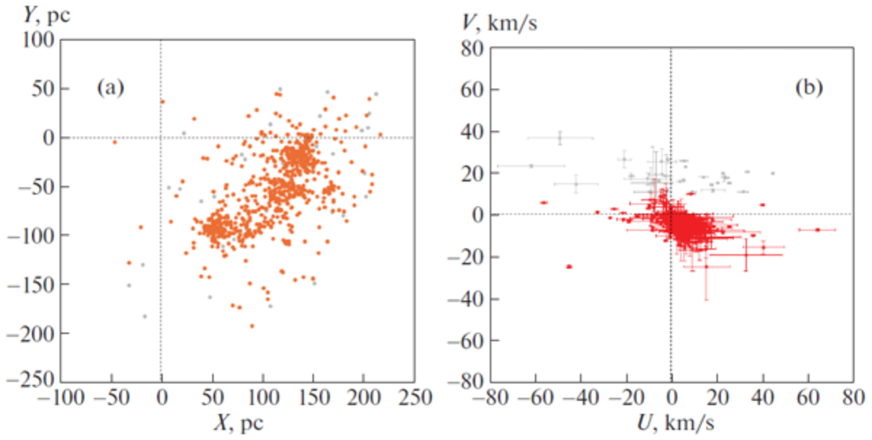
Figure 1: (a) Distribution of the probable members of the Scorpius–Centaurus association on the galactic plane $xy$; (b) spatial $UV$ velocities of these stars. The velocities are given relative to the LSR; the bright dots indicate the stars with velocities $V>10$ km/s.

3.1 Residual Velocities

In the residual velocity formation, the Sun’s peculiar velocity relative to the local standard of rest (LSR), $U_{\odot},$ $V_{\odot}$ and $W_{\odot}$ is primarily considered. The radial extension of the region under study (along $R$) is less than 200 pc; thus, there is no particular need to consider the Galaxy’s differential rotation, especially since the galactic rotation’s curve is nearly flat. However, it is interesting to consider the influence of the galactic spiral density wave. The expressions for taking these two effects into account are as follows:

$$\begin{array}[]{lll}V_{r}=V^{*}_{r}-[-U_{\odot}\cos b\cos l-V_{\odot}\cos b\sin l-W_{\odot}\sin b\\ +\tilde{v}_{\theta}\sin(l+\theta)\cos b-\tilde{v}_{R}\cos(l+\theta)\cos b],\end{array}$$ (2)

$$\begin{array}[]{lll}V_{l}=V^{*}_{l}-[U_{\odot}\sin l-V_{\odot}\cos l-r\Omega_{0}\cos b+\tilde{v}_{\theta}\cos(l+\theta)+\tilde{v}_{R}\sin(l+\theta)],\end{array}$$ (3)

$$\begin{array}[]{lll}V_{b}=V^{*}_{b}-[U_{\odot}\cos l\sin b+V_{\odot}\sin l\sin b-W_{\odot}\cos b\\ -\tilde{v}_{\theta}\sin(l+\theta)\sin b+\tilde{v}_{R}\cos(l+\theta)\sin b],\end{array}$$ (4)

where $V^{*}_{r},V^{*}_{l},V^{*}_{b}$ in the right-hand parts of the equations are the initial uncorrected velocities, and $V_{r},V_{l},V_{b}$ in the left-hand parts are the corrected velocities, using the ones in which the residual velocities $U,V,W$ based on relations (1) can be calculated; $R$ is the distance from the star to the galaxy’s rotation axis, $R^{2}=r^{2}\cos^{2}b-2R_{0}r\cos b\cos l+R^{2}_{0}.$

The distance $R_{0}$ is taken as $8.0\pm 0.15$ kpc [22]. The specific values of the Sun’s peculiar velocity relative to the LSR, $(U_{\odot},V_{\odot},W_{\odot})=(11.1,12.2,7.3)$ km/s, are taken in accordance with the definition [23].

There are two other velocities that are also of interest: the radial velocity $V_{R}$ oriented from the galactic center along the radius and the velocity $V_{\theta}$ orthogonal to it and directed along the galaxy’s rotation. These velocities are calculated based on the following relationships:

$$\begin{array}[]{lll}V_{\theta}=~{}~{}U\sin\theta+(V_{0}+V)\cos\theta,\\ V_{R}=-U\cos\theta+(V_{0}+V)\sin\theta,\end{array}$$ (5)

where the position angle $\theta$ satisfies the relation $\tan\theta=y/(R_{0}-x)$, $x,y,z$ are the rectangular heliocentric coordinates of the star; and $V_{0}$ is the linear velocity of the Galaxy’s rotation at a solar distance $R_{0}$.

Considering the influence of the spiral density wave, we used a model based on the linear theory of density waves by Lin and Shu [24], in which the potential’s perturbation has the form of a traveling wave.

$$\begin{array}[]{lll}\tilde{v}_{R}=f_{R}\cos\chi,\\ \tilde{v}_{\theta}=f_{\theta}\sin\chi,\\ \chi=m[\cot(i)\ln(R/R_{0})-\theta]+\chi_{\odot},\end{array}$$ (6)

where $f_{R}$ and $f_{\theta}$ are the perturbation amplitudes of the radial and azimuthal velocities; $i$ is the twist angle of spirals ($i<0$ for twisting spirals); $m$ is the number of arms; $\chi_{\odot}$ is the phase angle of the Sun, which is measured from the center of the Carina–Sagittarius Arm in this study; $\lambda$ is the distance (along the galactocentric radial direction) between the adjacent segments of spiral arms in a near-solar neighborhood (spiral wave length), which is calculated from the relation

$$\tan(i)=\lambda m/(2\pi R_{0}).$$ (7)

The described method for considering the influence of a spiral density wave was used, for example, in [25] or [26].

There is currently no certainty regarding the number of spiral arms $m$ in our galaxy. However, in this case, the neighborhood under consideration is small, and the position angle $\theta\rightarrow 0^{\circ}$ in formula (6). Under this condition, it can be easily shown that the inclusion of a spiral wave does not depend on $m$. Indeed, in accordance with relation (7), we have $\cot(i)=2\pi R_{0}/\lambda m.$. After substituting into (6), $m$ is canceled. Thus, considering the influence of a spiral density wave, it is necessary to have four parameters: $\lambda$, $f_{R}$, $f_{\theta}$ and $\chi_{\odot}.$

The assessment efficiency depends both on the perturbation amplitude of the spiral wave and on the solar phase in the wave. For example, at a certain phase value, a zero effect can be obtained even with a large amplitude. On the other hand, for a certain amplitude of radial perturbations, the value of the linear expansion coefficient $K$ from the stellar system decreases by the same amount. This was obtained in the kinematics analysis of the Gould belt [27].

In this paper, in accordance with the analysis of various star samples [28–31], the following parameters of the spiral density wave are adopted: $\lambda=2.2$ kpc, $f_{R}=5$ km/s, $f_{\theta}=0$ km/s and $\chi_{\odot}=-120^{\circ}.$ Since very young stars are considered, studies focused on the parameter values of the spiral density wave that were obtained by various authors for the youngest objects. For example, the value of the Sun’s phase in the density wave was found to be $\chi_{\odot}=-125\pm 10^{\circ}$ from the analysis of maser sources with measured trigonometric parallaxes [29], $\chi_{\odot}=-120\pm 10^{\circ}$ from a sample of young open star clusters [30], and $\chi_{\odot}=-121\pm 3^{\circ}$ from Cepheids [28]. The amplitudes of radial disturbance velocities $f_{R}$, as a rule, significantly differ from zero, while those of tangential $f_{\theta}$ do not [29, 30]. A current definition summary of $f_{R}$ and $f_{\theta}$ is provided by Loktin and Popova (Table 2 in [31]). Based on open-star cluster data from the current version of the “Uniform Catalog of Parameters of Open Star Clusters” and data from the Gaia DR2 catalog, these authors found $f_{R}=4.6\pm 0.7$ km/s and $f_{\theta}=1.1\pm 0.4$ km/s [31]. The value of the disturbance wavelength in the Sun’s vicinity lies in the range of 2.0–2.5 kpc [29–31]; it is well determined by both the positions of the stars and their kinematics. For example, the values $\lambda_{\theta}=2.3\pm 0.5$ kpc and $\lambda_{R}=2.2\pm 0.5$ kpc were found from the analysis of both tangential and radial velocities of young open star clusters from the Gaia DR2 catalog [30].

3.2 Residual Velocities Ellipsoid

To determine the parameters of the residual velocity ellipsoid of the stars, the following known method [32] is used. In the classic version, six moments of the second order $a,b,c,f,e,$ and $d$ are considered:

$$\begin{array}[]{lll}a=\langle U^{2}\rangle-\langle U^{2}_{\odot}\rangle,\qquad\quad b=\langle V^{2}\rangle-\langle V^{2}_{\odot}\rangle,\qquad\quad c=\langle W^{2}\rangle-\langle W^{2}_{\odot}\rangle,\\ f=\langle VW\rangle-\langle V_{\odot}W_{\odot}\rangle,\quad e=\langle WU\rangle-\langle W_{\odot}U_{\odot}\rangle,\quad d=\langle UV\rangle-\langle U_{\odot}V_{\odot}\rangle,\end{array}$$ (8)

As noted above, if necessary, the observable velocities can be released not only from the Sun’s peculiar motion, but also from the Galaxy’s differential rotation or from the influence of the spiral density wave. The moments $a,b,c,f,e,$ and $d$ are the coefficients of the surface equation

$$ax^{2}+by^{2}+cz^{2}+2fyz+2ezx+2dxy=1,$$ (9)

as well as the symmetric tensor components of residual velocity moments

$$\left(\matrix{a&d&e\cr d&b&f\cr e&f&c\cr}\right).$$ (10)

The values of all elements of this tensor can be determined from the solution of the following system of conditional equations:

$$\begin{array}[]{lll}V^{2}_{l}=a\sin^{2}l+b\cos^{2}l\sin^{2}l-2d\sin l\cos l,\end{array}$$ (11)

$$\begin{array}[]{lll}V^{2}_{b}=a\sin^{2}b\cos^{2}l+b\sin^{2}b\sin^{2}l+c\cos^{2}b\\ -2f\cos b\sin b\sin l-2e\cos b\sin b\cos l+2d\sin l\cos l\sin^{2}b,\end{array}$$ (12)

$$\begin{array}[]{lll}V_{l}V_{b}=a\sin l\cos l\sin b+b\sin l\cos l\sin b\\ +f\cos l\cos b-e\sin l\cos b+d(\sin^{2}l\sin b-\cos^{2}\sin b),\end{array}$$ (13)

$$\begin{array}[]{lll}V_{b}V_{r}=-a\cos^{2}l\cos b\sin b-b\sin^{2}l\sin b\cos b+c\sin b\cos b\\ +f(\cos^{2}b\sin l-\sin l\sin^{2}b)+e(\cos^{2}b\cos l-\cos l\sin^{2}b)\\ -d(\cos l\sin l\sin b\cos b+\sin l\cos l\cos b\sin b),\end{array}$$ (14)

$$\begin{array}[]{lll}V_{l}V_{r}=-a\cos b\cos l\sin l+b\cos b\cos l\sin l\\ +f\sin b\cos l-e\sin b\sin l+d(\cos b\cos^{2}l-\cos b\sin^{2}l).\end{array}$$ (15)

The solution is sought using the least squares method (LSM) with respect to six unknowns $a,b,c,f,e,$ and $d$. The eigenvalues of tensor (10) $\lambda_{1,2,3}$ are then found from the solution of the secular equation

$$\left|\matrix{a-\lambda&d&e\cr d&b-\lambda&f\cr e&f&c-\lambda\cr}\right|=0.$$ (16)

The eigenvalues of this equation are equal to the inverse values of the ellipsoid’s squared semiaxes of the velocity moments and, at the same time, to the ellipsoid’s squared semiaxes of the residual velocities:

$$\begin{array}[]{lll}\lambda_{1}=\sigma^{2}_{1},\lambda_{2}=\sigma^{2}_{2},\lambda_{3}=\sigma^{2}_{3},\\ \lambda_{1}>\lambda_{2}>\lambda_{3}.\end{array}$$ (17)

Directions of the principal axes of tensor (16) $L_{1,2,3}$ and $B_{1,2,3}$ are found from the relations

$$\tan L_{1,2,3}={{ef-(c-\lambda)d}\over{(b-\lambda)(c-\lambda)-f^{2}}},$$ (18)

$$\tan B_{1,2,3}={{(b-\lambda)e-df}\over{f^{2}-(b-\lambda)(c-\lambda)}}\cos L_{1,2,3}.$$ (19)

The errors of determining and are estimated according to the following procedure:

$$\begin{array}[]{lll}\displaystyle\varepsilon(L_{2})=\varepsilon(L_{3})={{\varepsilon(\overline{UV})}\over{a-b}},\quad\displaystyle\varepsilon(B_{2})=\varepsilon(\varphi)={{\varepsilon(\overline{UW})}\over{a-c}},\quad\displaystyle\varepsilon(B_{3})=\varepsilon(\psi)={{\varepsilon(\overline{VW})}\over{b-c}},\\ \displaystyle\varepsilon^{2}(L_{1})={\varphi^{2}\varepsilon^{2}(\psi)+\psi^{2}\varepsilon^{2}(\varphi)\over{(\varphi^{2}+\psi^{2})^{2}}},\quad\displaystyle\varepsilon^{2}(B_{1})={\sin^{2}L_{1}\varepsilon^{2}(\psi)+\cos^{2}L_{1}\varepsilon^{2}(L_{1})\over{(\sin^{2}L_{1}+\psi^{2})^{2}}},\end{array}$$ (20)

where $\varphi=\cot B_{1}\cos L_{1}$ and $\psi=\cot B_{1}\sin L_{1}.$ In this case, it is necessary to calculate beforehand three values $\overline{U^{2}V^{2}}$, $\overline{U^{2}W^{2}},$ and $\overline{V^{2}W^{2}},$ then

$$\begin{array}[]{lll}\displaystyle\varepsilon^{2}(\overline{UV})=(\overline{U^{2}V^{2}}-d^{2})/n,\quad\displaystyle\varepsilon^{2}(\overline{UW})=(\overline{U^{2}W^{2}}-e^{2})/n,\quad\displaystyle\varepsilon^{2}(\overline{VW})=(\overline{V^{2}W^{2}}-f^{2})/n,\end{array}$$ (21)

where $n$ is the number of stars. Here, the errors of each axis are estimated independently, with the exception of $L_{2}$ and $L_{3},$ in which its errors are calculated by one formula.

3.3 Kinematic Model

From the analysis of residual velocities $V_{r},V_{l},$ and $V_{b}$ the average group velocity $(U,V,W)_{\diamondsuit},$ can be determined, as well as four analogues of Oort constants $(A,B,C,K)_{\diamondsuit}.$ In this case, these characterize the effects of proper rotation ($A_{\diamondsuit}$ and $B_{\diamondsuit}$), as well as expansion and compression ($C_{\diamondsuit}$ and $K_{\diamondsuit}$), of the low-mass star sample. A simple kinematic model similar to the Oort–Lindblad model is used in this case [32]:

$$\begin{array}[]{lll}V_{r}=U_{\diamondsuit}\cos b\cos l+V_{\diamondsuit}\cos b\sin l+W_{\diamondsuit}\sin b\\ +rA_{\diamondsuit}\cos^{2}b\sin 2l+rC_{\diamondsuit}\cos^{2}b\cos 2l+rK_{\diamondsuit}\cos^{2}b,\end{array}$$ (22)

$$\begin{array}[]{lll}V_{l}=-U_{\diamondsuit}\sin l+V_{\diamondsuit}\cos l+rA_{\diamondsuit}\cos b\cos 2l-rC_{\diamondsuit}\cos b\sin 2l+rB_{\diamondsuit}\cos b,\end{array}$$ (23)

$$\begin{array}[]{lll}V_{b}=-U_{\diamondsuit}\cos l\sin b-V_{\diamondsuit}\sin l\sin b+W_{\diamondsuit}\cos b\\ -rA_{\diamondsuit}\sin b\cos b\sin 2l-rC_{\diamondsuit}\cos b\sin b\cos 2l-rK_{\diamondsuit}\cos b\sin b.\end{array}$$ (24)

The unknowns $(U,V,W)_{\diamondsuit}$ and $(A,B,C,K)_{\diamondsuit}$ result from a joint LSM solution of the conditional equation system (22)–(24). The following weight system is used: $w_{r}=S_{0}/\sqrt{S_{0}^{2}+\sigma^{2}_{V_{r}}},$ $w_{l}=S_{0}/\sqrt{S_{0}^{2}+\sigma^{2}_{V_{l}}}$ and $w_{b}=S_{0}/\sqrt{S_{0}^{2}+\sigma^{2}_{V_{b}}},$ where $S_{0}$ is the “space” dispersion; and $\sigma_{V_{r}},\sigma_{V_{l}},$ and $\sigma_{V_{b}}$ are the dispersions of the errors of the corresponding observed velocities. The value of $S_{0}$ is comparable to the mean-square residual (unit weight error) when solving conditional equations of the form (22)–(24). For the analysis of star residual velocities in this study, $S_{0}$ is taken as 3 km/s. The 3$\sigma$ criterion is applied for discarding residuals.

Using the parameter values $A_{\diamondsuit}$ and $C_{\diamondsuit},$ the $l_{xy}$ angle (vertex deviation) in accordance with the relation proposed by Parenago [33] is calculated:

$$\tan(2l_{xy})={{(AK-BC)_{\diamondsuit}}\over{(AB+KC)_{\diamondsuit}}},$$ (25)

in which the absence of expansion or compression (at $K=0$) takes a more familiar (as in the analysis of galactic rotation) form $\tan(2l_{xy})=-C_{\diamondsuit}/A_{\diamondsuit}.$ In the case of pure rotation, angle $l_{xy}$ points exactly at the kinematic center.

Note several important relationships in our kinematic model [32]:

$$\begin{array}[]{lll}(\Omega_{0})_{\diamondsuit}=(B-A)_{\diamondsuit},\\ (V^{\prime}_{0})_{\diamondsuit}=(B+A)_{\diamondsuit},\end{array}$$ (26)

where $(\Omega_{0})_{\diamondsuit}$ is the rotation’s angular velocity, and $(V^{\prime}_{0})_{\diamondsuit}=(\partial V_{\theta}/\partial R)_{\diamondsuit}$ is the first derivative of the linear rotational velocity $(V_{\theta})_{\diamondsuit}$ at the point $R=R_{0}.$

For the angular expansion and compression rate $(k_{0})_{\diamondsuit}$ and the first derivative of the linear radial velocity (oriented along the radius from the system’s kinematic center) of expansion and compression $V_{R}$ at the point $R=R_{0}$, studies show [32]

$$\begin{array}[]{lll}(k_{0})_{\diamondsuit}=(K-C)_{\diamondsuit},\\ (V^{\prime}_{R})_{\diamondsuit}=(K+C)_{\diamondsuit}.\end{array}$$ (27)

RESULTS AND DISCUSSION

Table 1 lists the results obtained by a joint LSM solution of the form’s conditional equations (22)–(24). The first column shows the sought-for parameters and their associated values; the second column gives the results obtained from the stars corrected for the Sun’s peculiar motion relative to the LSR; the third column gives the results obtained from the same stars with additional corrections to proper motions and radial velocities for the influence of a spiral density wave with amplitude $f_{R}=5$ km/s and the solar phase in the wave $\chi_{\odot}=-120^{\circ}$; the fourth column gives the results obtained from the stars described in the previous step, but all longitudes are corrected by $l=l-l_{xy},$ i.e., reduced to the new kinematic center of the system. In this new coordinate system, the values of the parameters $(U,V,W)_{\diamondsuit}$ and $(v,l,b)_{\diamondsuit}$ are not of great interest and thus are not listed here.

The lower part of the table shows the parameters of the residual velocity ellipsoid found as a LSM solution result of the conditional equation system (11)–(15). Based on the analysis of the Gaia catalog data by Wright and Mamajek (2018), the following average values of velocity dispersions were determined for the three main groups in the Scorpius–Centaurus association: $3.20^{+0.22}_{-0.20}$ km/s (US), $2.45^{+0.20}_{-0.20}$ km/s (UCL) and $2.15^{+0.47}_{-0.24}$ km/s (LCC). As observed in Table 1, the unit weight errors $\sigma_{0}$ (it has the sense of the average error over the three coordinate axes), as well as the dispersion values of the residual velocity ellipsoids, are in good agreement with the indicated estimates.

The second column in Table 1 gives the group velocity vector components of the sample relative to the Sun $({\overline{U}},{\overline{V}},{\overline{W}})=(-10.7,-16.1,-6.2)\pm(0.4,0.4,0.1)$ km/s. These were calculated as a simple average of the star velocities that were not corrected in any way.

In [18], the value $({\overline{U}},{\overline{V}},{\overline{W}})=(-11.8,-18.2,-6.1)\pm(0.8,0.8,0.3)$ km/s was obtained from the analysis of 134 bright members of the Scorpius–Centaurus association from the HIPPARCOS catalog [17]. Goldman et al. [35] determined $({\overline{U}},{\overline{V}},{\overline{W}})=(-8.2,-20.9,-6.1)\pm(1.1,1.5,0.6)$ km/s for 487 stars of subgroup C from LCC with an average age of 10 Ma. Wright and Mamajek [5] found $({\overline{U}},{\overline{V}},{\overline{W}})=(-7.2,-19.6,-6.1)\pm(0.2,0.2,0.1)$ km/s based on the analysis of approximately 250 bright members of the Scorpius–Centaurus association from the Gaia DR2 catalog.

Due to the fact that 33 stars with velocities $V>10$ km/s were discarded (Fig. 1), the sample is kinematically very homogeneous. Earlier, an estimate of the linear expansion coefficient $K=46\pm 8$ km/s/kpc was obtained from a sample of approximately 200 massive OB stars from the HIPPARCOS catalog [18]. Now, we obtain a significantly smaller error in determining this coefficient, $\pm$2 km/s/kpc. The value $K=41\pm 2$ km/s/kpc from the second column of Table 1 is in close agreement with the analysis of massive stars that was also obtained in [18] without considering the spiral density wave.

The value $l_{xy}=-13\pm 12^{\circ}$ (third column of Table 1) indicates that the kinematic center of the star system lies in the fourth galactic quadrant. However, the error in determining this quantity is large. On the other hand, the first axis direction of the residual velocity ellipsoid of the stars $L_{1}=324\pm 5^{\circ}$ (lower part of Table 1) is determined with a smaller error. Both $l_{xy}$ and $L_{1}$ alignments are counted from the direction toward the galactic center $l=0^{\circ}$ but in opposite ways. For their correct comparison, we will count from the direction $l=0^{\circ}$ uniformly. For example, for $L_{1}=324\pm 5^{\circ}$, we can write $324^{\circ}-360^{\circ}=-36^{\circ}$. Thus, the direction $-36\pm 5^{\circ}$ can be considered the direction toward the kinematic center of the Scorpius–Centaurus association.

Table 1: Parameters of the Oort–Lindblad kinematic model (upper part) and parameters of the residual velocity ellipsoid (lower part)

Parameters	Before accounting	After accounting	$l_{new}=l-l_{xy}$
${\overline{U}},$ km/s	$-10.67\pm 0.40$
${\overline{V}},$ km/s	$-16.14\pm 0.39$
${\overline{W}},$ km/s	$-6.19\pm 0.08$
$N_{\star}$	697	697	697
$\sigma_{0},$ km/s	2.2	2.2	2.2
$U_{\diamondsuit},$ km/s	$0.43\pm 0.40$	$2.55\pm 0.41$
$V_{\diamondsuit},$ km/s	$-3.94\pm 0.39$	$-3.43\pm 0.40$
$W_{\diamondsuit},$ km/s	$1.11\pm 0.08$	$1.11\pm 0.08$
$v_{\diamondsuit},$ km/s	$4.12\pm 0.38$	$4.42\pm 0.39$
$l_{\diamondsuit},$ deg	$276\pm 6$	$307\pm 5$
$b_{\diamondsuit},$ deg	$16\pm 2$	$15\pm 2$
$A_{\diamondsuit},$ km/s/kpc	$2.5\pm 2.0$	$2.0\pm 2.0$	$-0.1\pm 2.0$
$B_{\diamondsuit},$ km/s/kpc	$-2.0\pm 1.8$	$0.8\pm 1.9$	$0.8\pm 1.9$
$C_{\diamondsuit},$ km/s/kpc	$3.9\pm 1.9$	$-4.3\pm 1.9$	$-4.8\pm 2.0$
$K_{\diamondsuit},$ km/s/kpc	$41.1\pm 2.1$	$36.8\pm 2.1$	$36.8\pm 2.1$
$l_{xy},$ deg	$18\pm 12$	$-13\pm 12$	$0$
$\sigma_{1},$ km/s	$7.71\pm 0.62$	$8.23\pm 0.58$
$\sigma_{2},$ km/s	$2.40\pm 0.38$	$2.18\pm 0.41$
$\sigma_{3},$ km/s	$1.86\pm 0.24$	$1.58\pm 0.28$
$L_{1},B_{1},$ deg	$323\pm 7,~{}~{}3\pm 1$	$324\pm 5,~{}~{}2\pm 1$
$L_{3},B_{3},$ deg	$56\pm 9,~{}39\pm 3$	$60\pm 7,~{}68\pm 3$
$L_{2},B_{2},$ deg	$230\pm 9,~{}51\pm 2$	$233\pm 7,~{}22\pm 2$

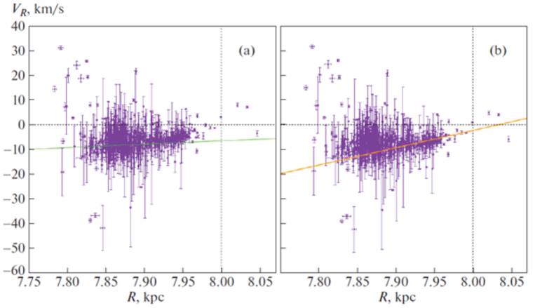
Figure 2: Galactocentric radial velocities of stars $V_{R}$ depending on the distance $R$ (a) corrected for the Sun’s motion relative to the LSR (the green line shows the influence of the spiral density wave) and (b) corrected for the Sun’s motion relative to the LSR with the influence of the spiral density wave taken into account (the orange line corresponds to $K$ effect found from these stars).

In the coordinate system with a new center (fourth column of Table 1), the constants $A_{\diamondsuit}$ and $C_{\diamondsuit}$ do not differ significantly from zero.

Figure 2 illustrates the stellar velocities $V_{R}$ depending on distance $R$. The velocities are corrected for the Sun’s motion relative to the LSR. Figure 2a shows a wave

$$-5\cos\biggl{[}-{2\pi R_{0}\over 2.2}\ln\biggl{(}{R\over R_{0}}\biggr{)}-120^{\circ}\biggr{]},$$

written down in accordance with relations (6) and (7), with the perturbation amplitude $f_{R}=5$ km/s, wavelength $\lambda=2.2$ kpc, and the solar phase in the wave $\chi_{\odot}=-120^{\circ}$; the minus sign before the formula means that the perturbation is oriented toward the center of the Galaxy in the center of a spiral arm (for example, when $R\approx 7.2$ kpc).

By definition, $2K=V_{R}/R+\partial V_{R}/\partial R$ if the rotational velocity $V_{\theta}$ is independent of the angle $\theta,$ $\partial V_{\theta}/\partial\theta=0$ [32]. At a constant angular velocity, i.e., at $\partial V_{R}/\partial R=0$, $\partial V_{R}/\partial R=0$ and $2K=V_{R}/R$. Figure 2b shows the dependence $V_{R}/R=2K$ with the value $K=37$ km/s/kpc.

Based on the solution from the fourth column of Table 1 using relation (27), $K-C=41.6\pm 2.8$ km/s/kpc and $K+C=32.0\pm 2.8$ km/s/kpc are found. From an observer’s perspective, these values show that there is a large angular velocity of expansion and a large positive derivative of the expansion’s linear velocity.

It is interesting to determine the kinematic parameters for US, UCL, and LCC separately. To do so, the entire sample was divided into three thirty-degree sectors by galactic longitude $l$. The results of solving equations (22)–(24), by allowing a spiral wave to influence three samples, are given in Table 2.

As can be seen in Table 2, the value of the linear expansion coefficient $K=13.6\pm 6.6$ km/s/kpc determined from the star samples with longitudes $l<300^{\circ}$ is very different from other results. These stars also have the highest unit weight error $\sigma_{0}.$ Thus, there is a strong influence from the stars of the first galactic quadrant, which are most likely background stars. Therefore, further analysis was carried out without these stars.

As a result, the LSM solution of conditional equations (22)–(24) was obtained under the condition $l>300^{\circ}$ using 574 stars, where the mean motion vector is $(U,V,W)_{\diamondsuit}=(2.96,-2.84,1.24)\pm(0.45,0.44,0.08)$ km/s (this vector corresponds to the total velocity $v_{\diamondsuit}=4.28\pm 0.43$ km/s with direction $l_{\diamondsuit}=316\pm 6^{\circ}$ and $b_{\diamondsuit}=17\pm 3^{\circ}$), as well as the following values of the remaining parameters:

$$\begin{array}[]{lll}A_{\diamondsuit}=-0.1\pm 2.1~{}\hbox{km/s/kpc},\\ B_{\diamondsuit}=1.5\pm 2.0~{}\hbox{km/s/kpc},\\ C_{\diamondsuit}=-9.5\pm 2.1~{}\hbox{km/s/kpc},\\ K_{\diamondsuit}=39.1\pm 2.3~{}\hbox{km/s/kpc},\\ l_{xy}=-1\pm 6^{\circ},\end{array}$$ (28)

where the unit weight error $\sigma_{0}$ amounted to 1.9 km/s. Based on the obtained value of the linear expansion coefficient $K=39\pm 2$ km/s/kpc, the characteristic time of expansion of the complex can be estimated according to the well-known formula $T=977.5/K$, $T=25\pm 2$ which is Myr.

To determine the rotation parameters, the star radial velocities are not necessary; two equations (23)–(24) or even one (23) are sufficient. Thus, to study the proper rotation of the Scorpius–Centaurus association, it would be better to use a catalog with a huge number of stars from Damiani et al. [3] when this directory appears in the Strasbourg database.

Table 2: Parameters of the Oort–Lindblad kinematic model found from the samples in three longitude intervals

Parameters	$l<300^{\circ}$	$l:300-330^{\circ}$	$l>330$
$N_{\star}$	116	213	367
$\sigma_{0},$ km/s	3.5	1.4	2.1
$U_{\diamondsuit},$ km/s	$4.5\pm 1.1$	$3.9\pm 0.6$	$4.0\pm 0.7$
$V_{\diamondsuit},$ km/s	$-3.1\pm 1.1$	$-5.1\pm 0.6$	$-1.8\pm 0.6$
$W_{\diamondsuit},$ km/s	$0.4\pm 0.3$	$1.3\pm 0.1$	$1.2\pm 0.1$
$v_{\diamondsuit},$ km/s	$5.5\pm 1.1$	$6.5\pm 0.6$	$4.6\pm 0.6$
$l_{\diamondsuit},$ deg	$326\pm 12$	$307\pm 5$	$335\pm 8$
$b_{\diamondsuit},$ deg	$4\pm 4$	$12\pm 2$	$15\pm 5$
$A_{\diamondsuit},$ km/s/kpc	$3.1\pm 6.1$	$15.2\pm 3.6$	$-11.7\pm 4.1$
$B_{\diamondsuit},$ km/s/kpc	$-11.3\pm 5.9$	$-11.7\pm 3.6$	$10.2\pm 4.1$
$C_{\diamondsuit},$ km/s/kpc	$-20.9\pm 6.3$	$12.1\pm 3.8$	$-25.9\pm 3.9$
$K_{\diamondsuit},$ km/s/kpc	$13.6\pm 6.6$	$37.6\pm 3.9$	$41.4\pm 4.0$
$l_{xy},$ deg	$16\pm 8$	$34\pm 5$	$5\pm 4$

As noted in the Data section, the sample contains approximately 5300 candidate members of the Scorpius– Centaurus association with their proper motions and parallaxes. The radial velocities are known for a small star fraction in this sample. In this case, the LSM solution of the three equation system (22)–(24) is followed as: a star with proper motions gives two equations (23) and (24); if the radial velocity is available, the star gives all three equations. With this approach, the rotation parameters are the main focus, assuming that the expansion parameter is already determined reliably.

As a result, the following solution was obtained: $(U,V,W)_{\diamondsuit}=(3.11,-1.88,1.10)\pm(0.17,0.13,0.02)$ km/s ($v_{\diamondsuit}=3.80\pm 0.15$ km/s with direction $l_{\diamondsuit}=329\pm 2^{\circ}$ and $b_{\diamondsuit}=17\pm 1^{\circ}$), and

$$\begin{array}[]{lll}A_{\diamondsuit}=1.8\pm 0.8~{}\hbox{km/s/kpc},\\ B_{\diamondsuit}=-7.5\pm 0.6~{}\hbox{km/s/kpc},\\ C_{\diamondsuit}=-9.6\pm 0.6~{}\hbox{km/s/kpc},\\ K_{\diamondsuit}=33.1\pm 0.9~{}\hbox{km/s/kpc},\\ l_{xy}=1\pm 2^{\circ},\end{array}$$ (29)

where $\sigma_{0}$ amounted to 1.3 km/s. Unlike solution (28), here, the values of all four constants are determined more accurately. The value $l_{xy}$ is close to zero, so there is no need to use a new coordinate system.

From the solution (29) with the dominant expansion, the following rotation parameters using the relation (26) are found: $(\Omega_{0})_{\diamondsuit}=-9.3\pm 1.0$ km/s/kpc and $(V^{\prime}_{0})_{\diamondsuit}=-5.7\pm 1.0$ km/s/kpc. The sign of this angular velocity indicates that its direction coincides with galactic rotation. At the point of the observer, the modulus of this velocity increases.

For the expansion, using relation (27), we find the following parameters: $(k_{0})_{\diamondsuit}=42.7\pm 1.1$ km/s/kpc and $(V^{\prime}_{R})_{\diamondsuit}=24.5\pm 1.1$ km/s/kpc. Thus, from the observer’s perspective, the modulus of this velocity also increases.

Applying a similar approach to solution (28), as well as to the solution in the last column of Table 1, similar values for the expansion parameters and the absence of proper rotation are found. Thus, the expansion parameters are determined reliably, and the parameters of proper rotation strongly depend on the adopted restrictions. However, in general, the proper rotation of the Scorpius–Centaurus association is small.

Fernández et al. [34] traced the kinematic evolution of the Scorpius–Centaurus association by analyzing the galactic orbits of various association parts in the past. The orbits were constructed in an axisymmetric potential with additional allowance for the spiral density wave. The expansion of the association was confirmed. Concurrently, the Local Bubble evolution was studied as well.

The studies by Wright and Mamajek [5] are also important to note. They tested the kinematics of the Scorpius–Centaurus association using several methods. In particular, they considered a method for searching for the linear expansion coefficient by the radial velocities of stars, and also reconstructed the star orbits in order to find the time point of their spatial concentration’s smallest area. The authors concluded that there was no evidence that the subgroups under consideration had a more compact configuration in the past. In other words, they found no expansion signs of the association. Conversely, Goldman and et al. [35] showed the presence of an expansion of the star subsystem in the association and in LCC with a linear expansion coefficient $K\sim 35$ km/s/kpc.

The following parameters of the residual velocity ellipsoid were found from the stars with radial velocities that were used to search for solution (28):

$$\begin{array}[]{lll}\sigma_{1}=7.72\pm 0.56~{}\hbox{km/s},\\ \sigma_{2}=1.87\pm 0.37~{}\hbox{km/s},\\ \sigma_{3}=1.74\pm 0.22~{}\hbox{km/s}\end{array}$$ (30)

and orientation parameters of this ellipsoid

$$\matrix{L_{1}=323\pm 7^{\circ},&B_{1}=~{}~{}3\pm 1^{\circ},\cr L_{2}=~{}54\pm 6^{\circ},&B_{2}=~{}12\pm 2^{\circ},\cr L_{3}=305\pm 6^{\circ},&B_{3}=~{}78\pm 2^{\circ}.\cr}$$ (31)

The direction $L_{1}=323^{\circ}(-37^{\circ})$ first agrees well with the direction towards the geometric center of the Scorpius-Centaurus association (Fig. 1) and, secondly, agrees well with the value $l_{xy}=-44^{\circ}$ found on the basis of the Oort–Lindblad model (solution (28)). In contrast to the ellipsoids of Table 1, it is interesting to note that this ellipsoid’s orientation is in excellent agreement with the Gould belt’s orientation [36]. For example, on the basis of a similar approach in Bobylev’s study [27], it was shown that the residual velocity ellipsoid of the Gould belt stars has principal semiaxes $\sigma_{1,2,3}=(8.9,5.6,3.0)\pm(0.1,0.2,0.1)$ km/s and it is located at an angle $22\pm 1^{\circ}$ to the galactic plane.

4 CONCLUSIONS

The kinematics of young T Tauri stars belonging to the Scorpius–Centaurus association was studied. For this purpose, the catalog of this star type was used, with their proper motions and parallaxes by Zari et al. [21] based on the Gaia DR2 catalog. The catalog [21] contains more than 23 000 stars and is dedicated to the stars belonging to the Gould belt.

Present studies mainly focus on the search for stars closely related to the Scorpius–Centaurus association. For this purpose, restrictions were placed on both the coordinates of the stars and their spatial velocities. The Oort–Lindblad kinematic model was used as the main model, in which the sample’s vector of the average group velocity relative to the LSR $(U,V,W)_{\diamondsuit}$ was determined, as well as four analogues of Oort constants $(A,B,C,K)_{\diamondsuit}$.

An important feature found in this study is the influence assessment of the spiral density wave. The assessment efficiency depends both on the amplitude of the perturbation of the spiral wave and on the solar phase in the wave. For example, at a certain value of the phase, a zero effect can be obtained even for a large amplitude. On the other hand, for a certain amplitude of radial perturbations, the linear expansion’s determined coefficient value of the stellar system $K_{\diamondsuit}$ decreases by the same amount. We have chosen a relatively small value of the radial perturbation amplitude and a zero value of the tangential perturbation amplitude found earlier from masers, OB stars, and young Cepheids.

First, a kinematic analysis was performed for about 700 Scorpius–Centaurus stars for which the proper motions, parallaxes, and radial velocities were measured. The new estimate of the linear expansion coefficient $K_{\diamondsuit}=39\pm 2$ km/s/kpc was obtained considering the Sun’s peculiar velocity relative to the LSR and the influence of the galactic spiral density wave with the amplitude of radial perturbations $f_{R}=5$ km/s and the solar phase in the wave $-120^{\circ}.$ Compared to the expansion, the proper rotation of the Scorpius–Centaurus association is small; it is poorly determined since the rotation parameters strongly depend on the adopted restrictions.

The residual velocity ellipsoid of the stars from this sample has the principal semiaxes $\sigma_{1,2,3}=(7.72,1.87,1.74)\pm(0.56,0.37,0.22)$ km/s and is positioned at an angle of $12\pm 2^{\circ}$ to the galactic plane. The orientation of the ellipsoid shows that it lies close to the Gould plane, and its first axis lies in the direction $143^{\circ}-323^{\circ}$.

Using approximately 5300 stars with their proper motions and parallaxes, it was shown that, relative to the LSR, the Scorpius–Centaurus association moves at a velocity $v_{\diamondsuit}=3.80\pm 0.15$ km/s in the direction $l_{\diamondsuit}=329\pm 2^{\circ}$ and $b_{\diamondsuit}=17\pm 1^{\circ}.$

ACKNOWLEDGEMENTS

The authors would like to thank the reviewer for useful comments, which helped improve the article.

FUNDING

The study was supported in part by the Program of the Presidium of the Russian Academy of Sciences KP19–270 “Questions of origin and evolution of the Universe using the methods of ground-based observations and space research.”

REFERENCES

1. A.G.A. Brown, A. Vallenari, T. Prusti, et al. (Gaia Collab.), Astron. Astrophys. 616, 1 (2018).

2. L. Lindegren, J. Hernandez, A. Bombrun, et al. (Gaia Collab.), Astron. Astrophys. 616, 2 (2018).

3. F. Damiani, L. Prisinzano, I. Pillitteri, et al., Astron. Astrophys. 623, 112 (2019).

4. P.T. de Zeeuw, R. Hoogerwerf, J.H.J. de Bruijne, et al., Astron. J. 117, 354 (1999).

5. N.J. Wright and E.E. Mamajek, Mon. Not. R. Astron. Soc. 476, 381 (2018).

6. V.A. Ambartsumian, Astron. Zh. 26 (3) (1949).

7. A. Blaauw, Bull. Astron. Inst. Netherland 11, 414 (1952).

8. A. Blaauw, Ann. Rev. Astron. Astrophys. 2, 213 (1964).

9. E. E. Mamajek, M. Meyer, and J. Liebert, Astron. J. 124, 1670 (2002).

10. M.J. Sartori, J.R.D. Lepine, and W. S. Dias, Astron. Astrophys. 404, 913 (2003).

11. T. Preibisch and E. Mamajek, in Handbook of Star Forming Regions, Ed. by Bo Reipurth, Vol. 5 of The Southern Sky ASP Monograph Publications (ASP, San Francisco, 2008), Vol. 2.

12. T. Cantat-Gaudin, C. Jordi, N.J. Wright, et al., Astron. Astrophys. 626, 17 (2019).

13. A. Rao, P. Gandhi, C. Knigge, et al., arXiv: 1908.00810 (2019).

14. A.M. Mel’nik and A.K. Dambis, Mon. Not. R. Astron. Soc. 472, 3887 (2017).

15. A.M. Mel’nik and A.K. Dambis, Astron. Rep. 62, 998 (2018).

16. T. Preibisch and H. Zinnecker, Astron. J. 117, 2381 (1999).

17. The HIPPARCOS and Tycho Catalogues, ESA SP– 1200 (1997).

18. V.V. Bobylev and A.T. Bajkova, Astron. Lett. 33, 571 (2007).

19. C.A.O. Torres, R. Quast, C.H.F. Melo, and M.F. Sterzik, in Handbook of Star Forming Regions, Ed. by Bo Reipurth, Vol. 5 of The Southern Sky ASP Monograph Publications (ASP, San Francisco, 2008), Vol. 2.

20. V.V. Bobylev and A.T. Bajkova, Astron. Lett. 39, 532 (2013).

21. E. Zari, H. Hashemi, A.G.A. Brown, et al., Astron. Astrophys. 620, 172 (2018).

22. T. Camarillo, M. Varun, M. Tyler, et al., Publ. Astron. Soc. Pacif. 130, 4101 (2018).

23. R. Schönrich, J. Binney, and W. Dehnen, Mon. Not. R. Astron. Soc. 403, 1829 (2010).

24. C.C. Lin and F.H. Shu, Astrophys. J. 140, 646 (1964).

25. Yu. N. Mishurov and I.A. Zenina, Astron. Astrophys. 341, 81 (1999).

26. D. Fernández, F. Figueras, and J. Torra, Astron. Astrophys. 372, 833 (2001).

27. V.V. Bobylev, Astron. Lett. 46 (2020, in press).

28. A.K. Dambis, L.N. Berdnikov, Yu. N. Efremov, et al., Astron. Lett. 41, 489 (2015).

29. A.S. Rastorguev, M.V. Zabolotskikh, A.K. Dambis, et al., Astrophys. Bull. 72, 122 (2017).

30. V.V. Bobylev and A.T. Bajkova, Astron. Lett. 45, 151 (2019).

31. A. V. Loktin and M. E. Popova, Astrophys. Bull. 74, 270 (2019).

32. K.F. Ogorodnikov, Dynamics of Stellar Systems (Pergamon, Oxford, 1965).

33. P.P. Parenago, Course of Stellar Astronomy (Gosizdat, Moscow, 1954) [in Russian].

34. D. Fernández, F. Figueras, and J. Torra, Astron. Astrophys. 480, 735 (2008).

35. B. Goldman, S. Roser, E. Schilbach, et al., Astrophys. J. 868, 32 (2018).

36. V.V. Bobylev, Astrophysics 57, 583 (2014).