Holding and transferring matter-wave solitons against gravity by spin-orbit-coupling tweezers

Abstract

We consider possibilities to grasp and drag one-dimensional solitons in two-component Bose-Einstein condensates (BECs), under the action of gravity, by tweezers induced by spatially confined spin-orbit (SO) coupling applied to the BEC, with the help of focused laser illumination. Solitons of two types are considered, semi-dipoles and mixed modes. We find critical values of the gravity force, up to which the solitons may be held or transferred by the tweezers. The dependence of the critical force on the magnitude and spatial extension of the localized SO interaction, as well as on the soliton’s norm and speed (in the transfer regime), are systematically studied by means of numerical methods, and analytically with the help of a quasi-particle approximation for the soliton. In particular, a noteworthy finding is that the critical gravity force increases with the increase of the transfer speed (i.e., moving solitons are more robust than quiescent ones). Nonstationary regimes are addressed too, by considering abrupt application of gravity to solitons created in the weightless setting. In that case, solitons feature damped shuttle motion, provided that the gravity force does not exceed a dynamical critical value, which is smaller than its static counterpart. The results may help to design gravimeters based on ultracold atoms.

I Introduction

Optical tweezers, which were first constructed in the classic works of Ashkin et al. Ashkin ; Chu for selecting and driving microscopic dielectric particles by means of laser beams, are nowadays used in various experiments aimed at trapping and transfer of atomic Bose-Einstein condensates (BECs) Steuernagel2005 -Nieminen2014 . Among these settings, is holding BEC under the action of gravity. The interaction of ultracold condensates with the gravitational field is a problem with applications to experiments in gravitational physics and development of precise measurement techniques. In particular, atomic Raman interferometry Fixler2007 -Xu2018 and Bloch oscillations Clade2005 -Poli2011 of ultracold atoms trapped in a vertical optical lattice were used for precise measurement of the free-fall acceleration, as well as its gradient, aimed at geological applications. A combination of these techniques was reported to remarkably improve the accuracy of atomic interferometry Fattori and fundamental measurements of gravity Charriere . Recently, a fountain gravimeter, which achieved a sub-$\mathrm{\mu}$G degree of accuracy, was fabricated on an atom chip Abend2016 , and a compact quantum gravimeter was realized in polarization-synthesized spin-dependent optical lattices Yongguan2018 -Robens2018 . Dynamics of BEC under the action of microgravity has also been a subject of many experiments microgravity -microgravity2 .

The self-attractive intrinsic nonlinearity of BEC, induced by inter-atomic collisions, which is accurately modeled by the Gross-Pitaevskii equation (GPE) GP , gives rise to self-trapped states, in the form of solitons recent-review and breathers Strathclyde . As concerns the above-mentioned topics, relevant aspects are manipulations of matter-wave solitons with the help of tweezers Carpentier2008 , motion of solitons Holtzmann -Rosanov2 and breathers Alodjants ; Rosanov3 driven by gravity, and Bloch oscillations of gap solitons in optical lattices under the action of a constant (gravity) force Salerno2008 . In this context, it is worthy to mention great diversity in the design of matter-wave interferometers offered by matter-wave solitons Rosanov4 -splitter .

However, the applications of optical tools to BEC are hampered by effects of heating the condensate by laser beams which are used for the creation of tweezers heating1 -heating3 and optical lattices OL-heating1 -OL-heating7 . In this work, we aim to elaborate a tweezers scheme for matter-wave solitons based on spatially localized spin-orbit (SO) coupling applied to BEC, by means of properly focused laser illumination. One of incentives for the introduction of the scheme is the fact that the SO interaction may be induced in the condensate without heating it no-heating1 -no-heating4 .

The configuration is schematically shown in Fig. 1, which assumes that the soliton is placed in a narrow vertical cigar-shaped potential trap and illuminated by a horizontal Raman laser beam inducing the SO coupling and focused on a segment of the vertical “cigar”. In fact, the focusing does not need to be very tight. Indeed, for a typical longitudinal extension of solitons, which is, normally, several microns Randy , the Raman-beam illumination should be confined on a comparable segment, which is, thus, much larger than the diffraction limit for the focusing, $\simeq\lambda/2$, as determined by the characteristic beam’s wavelength, $\lambda\simeq 1$ $\mathrm{\mu}$m Spielman ; Galitski .

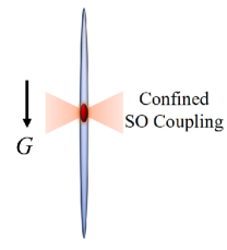
Figure 1: (Color online) The sketch of the setting: a quasi-1D matter-wave soliton, designated by the dark red color, is created in the vertical cigar-shaped potential trap, while horizontal beams, which induce the confined SO coupling, hold the soliton at a particular vertical position. ${\large G}$ represents the gravity force.

The SO coupling in BECs, which emulates the eponymous effect in physics of semiconductors, has been an active research subject in recent years Spielman -Yongping2016 . In the combination with the usual collision-induced nonlinearity, the SO coupling was theoretically shown to support various species of one-dimensional (1D) solitons 1D-SO-sol-1 -SKA0 . A surprising prediction is that the interplay of the linear SO interaction and cubic self-attraction leads to stabilization of multidimensional solitons in free space, which are completely unstable in the absence of the SO terms Sakaguchi2014 -Pangw2018 .

As concerns the application of the SO coupling to a spatially confined region, such as in the configuration sketched in Fig. 1, it was predicted that 1D solitons and their bound states may be maintained by means of localized SO interaction 1Dlocalized ; Bin2019 . Further, it was recently demonstrated that spatially confined SO coupling can be used to maintain stable 2D solitons Yongyao2018 . A related possibility is the use of effectively 1D and 2D (low-dimensional) SO coupling for the stabilization of, respectively, 2D and 3D solitons (in the full dimension), including a vortex component PRR .

The subject of the present work is the stability and dynamics of quasi-1D solitons held or transported by localized SO coupling against the action of gravity, as suggested by Fig. 1. The consideration is based on a combination of systematic numerical simulations and the use of an analytical approximation. The results may help to develop a new type of cold-atom gravimeter and, more generally, new techniques for precise measurements.

The remainder of the paper is structured as follows. The setting is introduced in Section II, which is followed by presentation of numerical and analytical results for stationary solitons, obtained in both quiescent and moving reference frames (the latter one pertaining to the transport of solitons), in Section III. Motion (shuttle oscillations) of solitons is numerically studied in Section IV, and the paper is concluded by Section V.

II The model

The setting sketched in Fig. 1, with the spatially confined SO coupling of the Rashba type Rashba , which can be created by the laser beam Campbell2011 , is represented by the following system of coupled GPEs for a pseudo-spinor (two-component) mean-field wave function, $\left(\psi_{+},\psi_{-}\right)$, written in the scaled form:

$$i\partial_{t}\psi_{+}=-{\frac{1}{2}}\partial_{xx}\psi_{+}+\Lambda(x)\partial_{x}\psi_{-}-(|\psi_{+}|^{2}+\gamma|\psi_{-}|^{2})\psi_{+}+{\frac{1}{2}}\frac{d{\Lambda}}{dx}\psi_{-}-Gx\psi_{+},$$

$$i\partial_{t}\psi_{-}=-{\frac{1}{2}}\partial_{xx}\psi_{-}-\Lambda(x)\partial_{x}\psi_{+}-(|\psi_{-}|^{2}+\gamma|\psi_{+}|^{2})\psi_{-}-{\frac{1}{2}}\frac{d{\Lambda}}{dx}\psi_{+}-Gx\psi_{-},$$ (1)

where the strength of the attractive self-interaction in each component is normalized to be $1$, $\gamma$ is the relative strength of the cross-interaction between the components, and $G$ is the gravity force. In the experiment, values of $G$ may be controlled by means of the angle between the direction of the quasi-1D trap holding the condensate and the vertical direction, as well as by running the experiment in microgravity settings microgravity ; microgravity2 . Because the natural transverse structure of laser beams is Gaussian, we adopt the corresponding shape of the spatial localization of the SO-coupling coefficient, cf. Refs. 1Dlocalized and Yongyao2018 :

$$\Lambda(x)=\Lambda_{0}\exp(-x^{2}/L^{2}),$$ (2)

where $L$ defines the confinement size, while amplitude $\Lambda_{0}$ may be fixed to $1$ by means of additional rescaling. Nevertheless, it is convenient to keep $\Lambda_{0}$ as a free parameter, to explore dependence of the predicted effects on the strength of the SO interaction.

Terms $\sim d\Lambda/dx$ in Eq. (1) appear when the GPE system is derived from the respective Hamiltonian,

$$H=\int_{-\infty}^{+\infty}\frac{1}{2}\left[\left(\left|\partial_{x}\psi_{+}\right|^{2}+\left|\partial_{x}\psi_{-}\right|^{2}-\left|\psi_{+}\right|^{4}-\left|\psi_{-}\right|^{4}\right)-\gamma\left|\psi_{+}\right|^{2}\left|\psi_{-}\right|^{2}\right.$$

$$+\frac{1}{2}\Lambda(x)\left(\psi_{+}^{\ast}\partial_{x}\psi_{-}-\psi_{-}^{\ast}\partial_{x}\psi_{+}+\psi_{+}\partial_{x}\psi_{-}^{\ast}-\psi_{-}\partial_{x}\psi_{+}^{\ast}\right)$$

$$\left.-Gx\left(\left|\psi_{+}\right|^{2}+\left|\psi_{-}\right|^{2}\right)\right]dx.$$ (3)

Solutions are characterized by their total norm, which is a dynamical invariant of the system,

$$N=\int_{-\infty}^{+\infty}dx\left(|\psi_{+}|^{2}+|\psi_{-}|^{2}\right).$$ (4)

Moving tweezers, which can transfer trapped solitons, are defined as profiles (2) moving at velocity $c$,

$$\Lambda(x)=\Lambda_{0}\exp\left[-\left(x-ct\right)^{2}/L^{2}\right].$$ (5)

In particular, we aim to find a critical value of velocity, up to which the trapped solitons may be stably transferred. This is a nontrivial issue because Eq. (1) is not Galilean invariant. To address it, we follow Ref. Sakaguchi2014 and rewrite Eqs. (1) in the moving reference frame, with coordinate $x^{\prime}=x-ct$ and transformed wave function, $\psi_{{\LARGE\pm}}\left(x,t\right)=\psi_{{\LARGE\pm}}^{\prime}\left(x^{\prime},t\right)\exp\left(icx^{\prime}+ic^{2}t/2+iGct^{2}/2\right)$:

$$i\partial_{t}\psi_{+}^{\prime}=-{\frac{1}{2}}\partial_{x^{\prime}x^{\prime}}\psi_{+}^{\prime}+\Lambda(x^{\prime})\partial_{x^{\prime}}\psi_{-}^{\prime}-(|\psi_{+}^{\prime}|^{2}+\gamma|\psi_{-}^{\prime}|^{2})\psi_{+}^{\prime}+\left[\frac{1}{2}{\frac{d\Lambda(x^{\prime})}{dx^{\prime}}+ic\Lambda}\left(x^{\prime}\right)\right]\psi_{-}^{\prime}-Gx^{\prime}\psi_{+}^{\prime},$$

$$i\partial_{t}\psi_{-}^{\prime}=-{\frac{1}{2}}\partial_{x^{\prime}x^{\prime}}\psi_{-}^{\prime}-\Lambda(x^{\prime})\partial_{x^{\prime}}\psi_{+}^{\prime}-(|\psi_{-}^{\prime}|^{2}+\gamma|\psi_{+}^{\prime}|^{2})\psi_{-}^{\prime}-\left[\frac{1}{2}{\frac{d\Lambda(x^{\prime})}{dx^{\prime}}+ic\Lambda}\left(x^{\prime}\right)\right]\psi_{+}^{\prime}-Gx^{\prime}\psi_{-}^{\prime}.$$ (6)

Thus, the underlying equations indeed change in the moving frame. Note that another transformation, $\psi_{\pm}^{\prime}\rightarrow\left(\psi_{\pm}^{\prime}\right)^{\ast}$, $t\rightarrow-t$, casts Eq. (6) into itself, with $c$ replaced by $-c$, thus making positive and negative values of $c$ mutually equivalent [see also Fig. 5(d) below].

The linear-mixing terms $\sim ic\Lambda$, which are generated by the transformation in Eq. (6), strongly affect the structure of solitons, but, generally, do not make them unstable, as shown below.

III Stationary solutions

III.1 Stationary states in the quiescent reference frame

III.1.1 Numerical results

In the 2D system, two types of fundamental solitons exist under the action of the SO coupling. One is built as a composite state including a fundamental soliton in component $\psi_{+}$ (one with zero topological charge, $S_{+}=0$), and a solitary vortex (with charge $S_{-}=1$) in component $\psi_{-}$. States of this type are classified as semivortex (SV) solitons Sakaguchi2014 (similar composite modes, found in a model with repulsive nonlinearity, were called “half vortices” BB2012 ). Due to the symmetry of the SO coupling, SVs with the opposite chirality, defined by the vorticity set $(S_{+}=-1,S_{-}=0)$, exist too. The other type of 2D fundamental solitons is the mixed-mode (MM) soliton, which is built as a superpositions of states with vorticities $(0,1)$ and $(-1,0)$ in the two components.

A 1D counterpart of the SV soliton is a semidipole (SD) composite state, which is composed of spatially even and odd modes in its two components, and can be found numerically starting from the following input:

$$\psi_{+}=A_{1}\exp(-x^{2}/W^{2}),~{}\psi_{-}=A_{2}\left(x/W\right)\exp(-x^{2}/W^{2}),$$ (7)

with width $W$ and real amplitudes $A_{1,2}$. A 1D version of MM solitons is built as a superposition of even and odd modes in both components Rongxuan2018 . Accordingly, the numerical search for such solutions may be initiated by input

$$\psi_{\pm}=\left[A_{1}\pm A_{2}\left(x/W\right)\right]\exp(-x^{2}/W^{2}).$$ (8)

The form of these is suggested by their 2D counterparts used in Ref. Sakaguchi2014 for constructing solitons of the SV and MM types.

In the numerical analysis, we chiefly focus on the Manakov’s nonlinearity, with $\gamma=1$ in Eq. (1) Manakov (although other values of $\gamma$ are considered too). This case is relevant for experimental realization of the SO coupling in binary mixtures of two different hyperfine atomic states Galitski -Yongping2016 , for which scattering lengths of collisions between atoms belonging to the same or different atomic states are nearly equal. The interplay of the SO coupling and nonlinearity of the Manakov’s type in the 2D system features special properties. In particular, the SD and MM solitons are included, in this case, in a broader family of 2D solitons with equal energies and equal chemical potentials for a fixed soliton’s norm (4) Sakaguchi2014 . A systematic numerical analysis demonstrates below that states maintained by the SO trap (2) are especially robust against the effect of gravity in the system with the Manakov’s nonlinearity.

Stationary solutions of Eq. (1) for solitons can be obtained as follows.

(i) Use the imaginary-time method (ITM) Chiofalo2000 ; JKyang2008 to produce a stationary solution at $G=0$. Because the SD and MM solitons represent mutually degenerate ground states in the Manakov’s case, either of them can be generated by the ITM with inputs chosen as per Eqs. (7) and (8), respectively (at $\gamma<1$ and $\gamma>1$, the ground state is represented by solitons of the SD and MM types, respectively Sakaguchi2014 ). Due to the SO coupling between the component of the soliton, they share a common value of the chemical potential $\mu$, taking the form of

$$\psi_{\pm}(x,t)=\phi_{\pm}(x)e^{-i\mu t}.$$ (9)

The chemical potential of the ITM-produced solutions can be accurately identified by the substitution of the solutions in Eq. (1) and looking at the central point ($x=0$).

(ii) Use the wave function and chemical potential of the solution with $G=0$ as an initial guess, and then apply the squared-operator method (SOM) JKyang2007 , to produce a stationary solution with $G^{(1)}=\delta G$, where $\delta G$ is a small value.

(iii) Using SOM, continue to build solutions, increasing the gravity force by small steps, $G^{(n-1)}\rightarrow G^{(n)}=G^{(n-1)}+\delta G$.

In the case of $G>0$, the formal ground state (the one with the minimal energy) corresponds to the free fall of the wave packet towards $x\rightarrow\infty$. For this reason, ITM, which seeks for the system’s ground state, is irrelevant for constructing solitons at $G>0$, and it was necessary to use SOM at stages (ii) and (iii).

Figures 2(a,b) display typical examples of stable MM and SD solitons, obtained by means of this procedure for different values of $G$ and fixed $\mu$. Stability of these solitons is illustrated by direct simulations displayed in panel (c). The results show that the shape of MM solitons quickly tends to become close to the SD type with the increase of $G$, therefore the consideration is focused below, chiefly, on the SD modes.

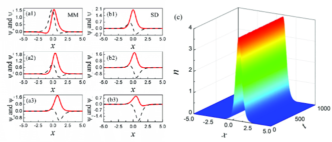
Figure 2: Continuous and dashed lines depict two components of stationary wave functions in stable solitons of the MM and SD types [the left column, (a1)-(a3), and the right one, (b1)-(b3), respectively] for different values of the gravity force: $G=0$ (a1,b1), $0.12$ (a2,b2), and $0.24$ (a3,b3). The solutions are obtained with a fixed chemical potential, $\mu=-2.5231$, starting from the MM and SD solitons with norm $N=4$ [see Eq. (4)] at $G=0$. Solid and dashed curves in these panels represent profiles of the $\psi_{+}$ and $\psi_{-}$ components, respectively. (c) Stability of the solitons (of the MM type, as concerns this example) in direct simulations, for $G=0.24$. The soliton was initially perturbed by random noise, added at the $3\%$ amplitude level. The evolution is shown by the spatiotemporal distribution of the total density, $n(x,t)=|\psi_{+}(x,t)|^{2}+|\psi_{-}(x,t)|^{2}$. In this figure, parameters of Eqs. (1) and (2) are fixed as $\gamma=1$ and $L=2$.

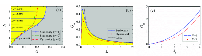
Figure 3: (a) Stability and instability areas (yellow and gray ones, respectively) of stationary states in the $\left(N,G\right)$ plane for $\gamma=1$. Here, the source soliton used at $G=0$ is one of the SD type, and branches with $\mu=-0.5428$, $-0.9247$, $-1.6455$, $-2.5231$, $-3.6451$ represent solution families starting with norms $N=1,2,3,4,5$ at $G=0$, respectively. The green dashed curve is the stability boundary for $\gamma=0$. Here and in panel (b), the red dashed-dotted curve is the stability boundary of the shuttle-motion regime, which is considered below. The SO confinement size is fixed in this panel as $L=2$, see Eq. (2). (b) The stability and instability areas of stationary states in the $\left(G,L\right)$ plane, for fixed norm $N=5$. The dotted line is the fitting curve, which is $G_{\mathrm{cr}}=0.6/L$. (c) $G_{\mathrm{cr}}$ as a function of $\Lambda_{0}$ for $N=4$ (solid curve) and $N=3$ (dashed curve) for $(L,\gamma)=(2,1)$.

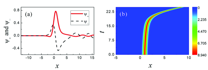
Figure 4: (a) A delocalized solution with nonvanishing tails, atr $(N,G,L)=(2,0.14,2)$. (b) The evolution of an unstable soliton, with parameters $(N,G,L)=(6,0.28,2)$.

Results of the numerical analysis are summarized in Fig. 3. First, panel (a) displays a stability area for the stationary soliton solutions in the $(N,G)$ plane. They exist and are stable in the yellow area, between $G=0$ and the critical (largest) value $G=G_{\mathrm{cr}}$. Horizontal lines connecting points $G=0$ and $G=G_{\mathrm{cr}}$ show that the variation of $G$ at fixed values of the chemical potential, $\mu$, practically does not affect the respective value of the soliton’s norm, $N$. At $G>G_{\mathrm{cr}}$, solutions with $N<3$ become delocalized, developing nonvanishing tails which extend to the boundary of the integration domain, see Fig. 4(a). This result implies that, under the action of strong gravity, the condensate leaks from the finite region at which the SO coupling is applied. Further, in the interval of $3<N<5$, at $G>G_{\mathrm{cr}}$ the numerical procedure yields only zero solution, while unstable solitons are obtained for $N>5$ and $G-G_{\mathrm{cr}}$ positive but not too large. As shown in Fig. 4(b), unstable solitons eventually escape from the trap and start the free fall towards $x\rightarrow+\infty$. Only zero solution is produced by the numerical method at any value of $N$ for $G-G_{\mathrm{cr}}$ large enough. In the case of $\gamma=1$ (the Manakov’s nonlinearity), values of $G_{\mathrm{cr}}$ for the SD and MM solitons are naturally found to be identical. Typical examples of such stable solitons at the boundary of their stability area are shown in Figs. 2(a3,b3).

Figure 3(a) clearly demonstrates that the stability area expands with the increase of $N$, hence stronger nonlinearity makes the solitons more stable against the action of the gravity. Additional numerical results reveal that $G_{\mathrm{cr}}$ is smaller at both $\gamma<1$ and $\gamma>1$ than in the Manakov’s case. In particular, Fig. 3(a) shows the $G_{\mathrm{cr}}(N)$ curve for $\gamma=0$, with values $G_{\mathrm{cr}}$ essentially smaller than for $\gamma=1$. Thus, as mentioned above, the Manakov’s nonlinearity is optimal for the stabilization of the solitons against gravity. Indeed, it is natural to expect that effects of the SO coupling are strongest when the nonlinearity is equal for the nonlinear self- and cross-interactions of components of the pseudo-spinor wave function.

Further, Fig. 3(b) shows the dependence of $G_{\mathrm{cr}}$ on size $L$ of the confinement region in which the SO coupling is applied, as per Eq. (2), for the SD soliton with $N=5$. The dependence features a maximum at $L\approx 0.6$, which is, quite naturally, comparable to the width of the corresponding soliton, $W\simeq$ $\sim 0.3$. The numerical results demonstrate that $G_{\mathrm{cr}}$ decays as $L^{-1}$ with the increase of $L$. This finding is explained below by means of the analytical approximation, see Eq. (15).

Finally, the growth of $G_{\mathrm{cr}}$ with the increase of the strength of the localized SO-coupling term, i.e., $\Lambda_{0}$ in Eq. (2), is displayed in Fig. 3(c). Roughly linear initial increase of $G_{\mathrm{cr}}$ with $\Lambda$, as well as its increase with $N$, observed in the figure, also complies with Eq. (15) derived below. The increase of $\Lambda_{0}$ leads not only to the growth of critical gravity force, $G_{\mathrm{cr}}$, but also to growth of the amplitude of the nonzero tail of the wave function extending towards the right edge of the solution domain at $G>G_{\mathrm{cr}}$ (not shown here in detail).

III.1.2 The analytical approximation

Characteristics of the stationary state under the combined action of gravity and SO-coupling-induced trap may be analyzed by means of the approximation which treats the soliton as a quasi-particle. To illustrate the application of the approximation in a simple form, in Appendix we formulate it for the simplest setting based on the single GPE, with the localized trap represented by an attractive delta-functional potential. Here we apply similar analysis to the system under the consideration.

If the soliton’s width is $\lesssim L$, then the effective soliton’s potential, induced by the localized SO coupling as per Eq. (3), is approximated as

$$U_{\mathrm{SOC}}(\xi)=-U_{0}\Lambda_{0}N^{2}\exp\left(-\xi^{2}/L^{2}\right),$$ (10)

cf. Eq. (A5), where $\xi$ is the coordinate of the soliton’s center, $U_{0}$ is a constant, and use is made of the fact that the soliton’s width and norm scale with its amplitude $A$ as $W\sim A^{-1}$ and $N\sim A^{2}W$ . This potential gives rise to the trapping force,

$$F_{\mathrm{SOC}}(\xi)=-\frac{dU_{\mathrm{SOC}}(\xi)}{d\xi}=-2U_{0}\Lambda_{0}N^{2}\left(\xi/L^{2}\right)\exp\left(-\xi^{2}/L^{2}\right).$$ (11)

The maximum value of the force is attained at the value of $\xi$ determined by condition

$$\frac{dF_{\mathrm{SOC}}(\xi)}{d\xi}=0,~{}\mathrm{i.e.},~{}\xi_{\max}^{2}=L^{2}/2,$$ (12)

and accordingly, the largest absolute value of the force corresponds to

$$\left(F_{\mathrm{SOC}}(\xi)\right)_{\max}=-\sqrt{2/e}U_{0}\Lambda_{0}N^{2}L^{-1}.$$ (13)

The competing gravity force acting on the soliton is estimated as

$$F_{G}=F_{0}NG,$$ (14)

where $F_{0}$ is another constant. Finally, the largest value of $G$, up to which the equilibrium condition, $F_{\mathrm{SOC}}(\xi)+F_{G}=0$, may hold, is

$$G_{\mathrm{cr}}=\sqrt{\frac{2}{e}}\frac{U_{0}\Lambda_{0}}{F_{0}}\frac{N}{L},$$ (15)

cf. Eqs. (A6) and (A7) in appendix. Equation (15) explains the above-mentioned $L^{-1}$ dependence for relatively large $L$. On the other hand, if $L$ is too small, the SO-coupling trap is obviously weak, therefore $G_{\mathrm{cr}}$ vanishes at $L\rightarrow 0$.

III.2 Stationary states in the moving reference frame

Stationary solutions in the moving reference frame were obtained by solving Eq. (6) with velocity $c\neq 0$. The procedure is similar to that outlined above for $c=0$:

(i) For a given value of $c$, ITM is used to produce a stationary solution with $G=0$, as the ground state.

(ii) Stable solitons with $G\neq 0$ are obtained by means of the continuation of the latter solution by small steps to $G>0$, with the help of SOM because, as well as in the case of $c=0$, the stationary soliton cannot be a ground state at $G>0$.

An example of a stable soliton with $c\neq 0$ is displayed in Figs. 5(a1,a2). The stability is corroborated by direct simulations of the perturbed evolution, as shown in Fig. 5(b). Comparison of the field profiles displayed in Fig. 5(a) with their counterparts, shown in Fig. 2(b2) for the same values $N=4$ and $G=0.12$, but zero velocity, demonstrates that the moving soliton, remaining a stable solution, develops a complex structure, in comparison with the essentially real one at $c=0$. On the other hand, Fig. 5(c) suggests that the total-density profile of the moving soliton, shown in terms of $n(x^{\prime})=|\phi_{+}(x^{\prime})|^{2}+|\phi_{-}(x^{\prime})|^{2}$, varies quite slowly with the increase of the velocity at a fixed value of the total norm. The latter figure demonstrates that the overall shape of the soliton gradually becomes sharper, which enhances the strength of trapping by the localized SO coupling.

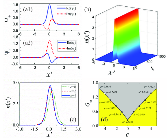
Figure 5: (a1,a2) Real and imaginary parts of two components of a composite soliton of the SD type in the moving reference frame, with speed $c=4$, at $G=0.12$. (b) Direct simulations of the evolution of the soliton perturbed by random noise at the $3\%$ amplitude level, which confirms its stability. The evolution is shown by means of the spatiotemporal distribution of the total density, $n(x^{\prime},t)$. (c) Total-density profiles of the stationary solitons with a fixed value of the total norm, $N=4$, and different values of velocity $c$. (d) The stability area (the yellow one), $G\leq G_{\mathrm{cr}}$, of the stationary solitons in the $(c,G)$ plane. In all the panels, the parameters are fixed as $(N,L,\gamma)=(4,2,1)$.

Stability of the moving solitons of the SD type is summarized in the parameter chart in the $\left(c,G\right)$ plane, which is displayed in Fig. 5(d). The symmetry of the stability area with respect to $c\longleftrightarrow-c$ corresponds to the above-mentioned invariance of Eq. (6) for the replacement of $c$ by $-c$. The figure demonstrates that the increase of $|c|$ leads to additional stabilization of the trapped solitons (growth of $G_{\mathrm{cr}}$). This effect may be explained by the fact that the linear-mixing terms $\sim ic\Lambda\left(x^{\prime}\right)$ in Eq. (6), being proportional to the spatial-modulation coefficient, $\Lambda(x)$, induce an additional effective potential which enhances the trapping action of the spatially confined SO coupling. In particular, considering stationary solutions to Eq. (6), $\psi_{\pm}^{{}^{\prime}}=\exp\left(-i\mu t\right)\phi_{\pm}(x^{\prime})$, with $\left|\phi_{\_}\right|\ll\left|\phi_{+}\right|$, and focusing on the effect of terms $\sim{ic\Lambda}\left(x^{\prime}\right)$ (neglecting, for the time being, terms $\sim d\Lambda(x^{\prime})/dx^{\prime}$), the use of the second equation in system (6) makes it possible to eliminate $\phi_{-}$ in favor of $\phi_{+}$, as $\phi_{-}\approx-ic\mu^{-1}\Lambda(x)\phi_{+}$. Then, the substitution of this result in the first equation of system (6) produces an effective potential,

$$U_{\mathrm{eff}}(x)\approx c^{2}\mu^{-1}\Lambda^{2}(x).$$ (16)

Because soliton states exist at $\mu<0$, the potential given by Eq. (16) is indeed a trapping one, with the negative sign, thus helping to additionally stabilize the bound state. The action of the extra potential also explains the shift of the overall-density profile back towards $x=0$ and sharpening of the profile with the increase of $c$ in Fig. 5(c).

Figure 6: (a,b) Profiles of the two components of the moving soliton with the same values $(N,L,\gamma)=(4,2,1)$ as in Fig. 5(a1,a2,c), but much larger gravity force, $G=1.36$ (instead of $G=0.12$ in Fig. 5). This soliton is located close to the stability boundary, in terms of Fig. Fig. 5(d). (c) The comparison of the total density of the same soliton (the red short dotted curves) and its counterpart pertaining to $G=0.12$ (the solid black line).

Lastly, while the moving solitons shown in Fig. 5(a1,a2,c) are located deep inside the stability area, in terms of Fig. 5(d), Fig. 6 displays an example of a soliton with the same values of the norm, $N=4$, and speed, $c=4$, but taken at a much stronger gravity force ($G=1.36$ instead of $G=0.12$), which places the soliton close to the stability boundary. Comparison of the latter profile with its counterpart from Fig. 5(a1,a2), see panel (c) in Fig. 6, provides another proof of the robustness of the solitons: the increase of $G$ by a factor $\approx 11.3$ leads to a minor change in the shape, viz., reduction of the overall peak density by a factor $\approx 0.81$, and a shift of the peak towards $x>0$.

IV Dynamical solutions

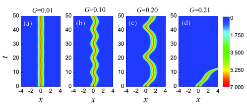
Figure 7: Direct simulation initiated by the abrupt application of gravity, with strength $G=0.01$ (a), $0.10$ (b), $0.20$ (c), and $0.21$ (d), to a soliton of the MM type, originally created for $G=0$. Other parameters are $(N,L,\gamma)=(5,2,1)$. The evolution is shown by means of spatiotemporal distributions of the total density.

The dynamics of solitons in the present system may be tested by abruptly applying gravity to a mode created in a weightless environment, i.e., generated by Eq. (1) with $G=0$ (in the experiment, this may be realized by creating a soliton in a horizontally oriented cigar-shaped trap, which is then quickly turned in the vertical plane). Figure 7 exhibits a typical example of the subsequent evolution of a soliton of the MM type, under the action of the suddenly applied gravity with different values of $G$. It is seen that the soliton develops shuttle motion with an amplitude and period depending on $G$ (oscillatory motion of nonlinear SO-coupled wave packets in a trapping potential was considered in Ref. Mardonov ). The resulting period of the shuttle motion for the SD and MM solitons is shown in Fig. 8 as a function of $G$. The figure demonstrates that solitons of both types develop identical dynamics in the case of the Manakov’s nonlinearity, $\gamma=1$. The divergence of the period at the critical value, $G=G_{\mathrm{cr}}^{\mathrm{d}}$, implies that, at $G>G_{\mathrm{cr}}^{\mathrm{d}}$, the soliton can no longer be held in the shuttle state by the spatially confined SO-coupling trap, see an example in Fig. 7(d)]. The dynamical critical value of the gravity strength, $G_{\mathrm{cr}}^{\mathrm{d}}$, is presented, as a function of $N$ and $L$, in Figs. 3(a,b). Shapes of dependences $G_{\mathrm{cr}}^{\mathrm{d}}(N)$ and $G_{\mathrm{cr}}^{\mathrm{d}}(L)$ are similar to their counterparts for the stationary solutions, while the magnitude of $G_{\mathrm{cr}}^{\mathrm{d}}$ is, naturally, smaller, as maintaining stable solitons in the dynamical regime requires to add some margin to the critical value defined for the static state.

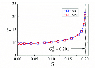
Figure 8: Period $T$ of the shuttle motion of solitons originally created with $G=0$ and then abruptly set in motion by the application of gravity force $G$. Dependences $T(G)$ are shown for solitons of the SD and MM types, with parameters $(N,L,\gamma)=(5,2,1)$. Note that the periods are fully identical for both types of the solitons in the case of $\gamma=1$ (the Manakov’s nonlinearity). The soliton ecapes from the shuttle regime at $G>G_{\mathrm{cr}}^{\mathrm{d}}$.

Long-time dynamics in the shuttle regime may be characterized by the soliton’s center-of-mass coordinate, defined as

$$X_{\mathrm{mc}}(t)={N}^{-1}\int_{-\infty}^{+\infty}(|\psi_{+}(t)|^{2}+|\psi_{-}(t)|^{2})xdx.$$ (17)

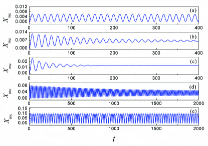
Figure 9: (a,b,c) Motion of the center of mass of the MM soliton, originally created with parameters $(N,\gamma,G_{0})=(1,1,0)$, under the action of the suddenly applied gravity with $G=0.01$ (a), $0.02$ (b) and $0.04$ (c). (d) The same, but for initial parameters $(N,\gamma,G_{0})=(3,1,0)$ and $G=0.16$. (e) The same for $(N,\gamma,G_{0})=(5,1,0)$ and $G=0.2$. In all the cases, coefficients of the confined SO-coupling term in Eq. (2) are $\Lambda_{0}=1$ and $L=2$.

Figure 9 displays the long-time regimes of motion produced by simulations performed for different values of parameters $N$ and $G$. It is observed that the oscillations are, generally, damped, which may be explained by weak radiation losses of the soliton moving with acceleration RMP . The damping rate increases with the increase of $G$ and decrease of $N$. The former peculiarity is explained by the fact that rapid oscillations at smaller values of $G$ (see Fig. 8) produce little radiation RMP , while, on the other hand, heavier solitons with a larger norm are less amenable to the action of the weak recoil force produced by the emission of radiation.

V Conclusion

The objective of this work is to study the dynamics of two-component matter-wave solitons under the action of the gravity field, with the aim to hold the solitons in a fixed position, or move them at a constant speed, by means of an effective trapping potential imposed by the spatially confined SO (spin-orbit) coupling. In comparison with usual laser-beam tweezers, advantage offered by the SO-coupling trap is the absence of detrimental heating effects. First, stationary solutions of the system of coupled GPEs for solitons of the SD (semi-discrete) and MM (mixed-mode) types were produced, in the quiescent and moving reference frames. In both cases, the critical value of the gravity force, $G_{\mathrm{cr}}$, which is the boundary of the stability area for the solitons trapped by the localized SO coupling, was found. By means of systematically collected numerical results and the analytical approximation, which treats the soliton as a quasi-particle, it was demonstrated that the stability area can be expanded (i.e., $G_{\mathrm{cr}}$ made larger) by increasing the strength of the SO-coupling term, the norm, and the speed, in the case of the moving system. In the second part of the work, dynamical regimes were addressed, by abruptly applying gravity to solitons created in the weightless setting. If the gravity force is smaller than the respective dynamical critical value (which, in turn, is smaller than its stationary counterpart), the solitons feature damped shuttle motion, with the period and damping rate affected by the gravity strength. The results produced by the consideration of both stationary and dynamical settings demonstrate the ability of the effective trapping potential, induced by the spatially confined SO coupling, to hold solitons against the gravity, and transfer them at a constant speed, the latter regime being actually more stable. These findings may help to design new gravimeters and improve other techniques for precise measurements, based on the use of cold atoms.

The present analysis may be extended in other directions. First, a natural possibility is to consider this problem in the 2D geometry, where conditions for the soliton stability are drastically different from those in the 1D case Sakaguchi2014 -Pangw2018 . The 2D matter-wave solitons stabilized by the SO coupling include vortex components, which suggests a possibility to consider the interaction of vortex solitons with gravity. Further, one can add the beyond-mean-field Lee-Huang-Yang corrections to the GPE system Petrov , and thus consider holding and transfer of “quantum droplets” (self-trapped modes with the flat-top shape Petrov ; recent-review ) in the presence of gravity. Note that the interplay between the spatially uniform SO coupling and LHY corrections was considered in Refs. Cui2018 ; QD2017 ; ZW2013 . A challenging option is to extend the current setting to the full 3D geometry.

Appendix: The analytical approximation in the simplest form

The single GPE, which includes the gravity field and the localized trap represented by the $\delta$-functional attractive potential with strength $\varepsilon>0$ (such as one induced by a tightly focused red-shifted laser beam), is

$$i\partial_{t}\psi=-{\frac{1}{2}}\partial_{xx}\psi-|\psi|^{2}\psi-Gx\psi-\varepsilon\delta(x)\psi.$$ (A1)

Here the localized potential is set at $x=0$ without the loss of generality. The Hamiltonian corresponding to Eq. (A1) is

$$H=\int_{-\infty}^{+\infty}\left[\frac{1}{2}\left(\left|\partial_{x}\psi\right|^{2}-\left|\psi\right|^{4}\right)-Gx\left|\psi\right|^{2}\right]dx-\varepsilon|\psi(x=0)|^{2},$$ (A2)

cf. Eq. (3). Stationary solutions to Eq. (A1), with chemical potential $\mu$, are looked form as $\psi=\exp\left(-i\mu t\right)\phi(x)$, where real function $\phi(x)$ obeys equation

$$\mu\phi=-{\frac{1}{2}}\frac{d^{2}\phi}{dx^{2}}-\phi^{3}-Gx\phi-\varepsilon\delta(x)\phi.$$ (A3)

In the absence of the gravity and trapping potential, the commonly known nonlinear-Schrödinger soliton with norm $N$, $\mu=-N^{2}/8$, and central coordinate $\xi$, is

$$\phi_{\mathrm{sol}}(x)=(N/2)\mathrm{sech}\left((N/2)\left(x-\xi\right)\right).$$ (A4)

If the gravitational and trapping potentials in Eq. (A2) are considered as small perturbations, the respective terms in the soliton’s energy are

$$U_{\varepsilon}(\xi)+U_{G}(\xi)=-\left(N/2\right)^{2}\varepsilon~{}\mathrm{sech}^{2}\left(N\xi/2\right)-GN\xi,$$ (A5)

which predicts a stationary state at a local minimum of the potential, defined by $\left(d/d\xi\right)\left(U_{G}(\xi)+U_{\varepsilon}(\xi)\right)=0$, i.e., at $\xi$ which is a smaller root of the equation

$$\tanh\left(\frac{N}{2}\xi\right)-\tanh^{3}\left(\frac{N}{2}\xi\right)=\frac{4G}{\varepsilon N^{2}}.$$ (A6)

As follows from Eq. (A6), the stationary state exists at values of the gravity force

$$G\leq G_{\mathrm{cr}}=\frac{\varepsilon N^{2}}{6\sqrt{3}}.$$ (A7)

Alternatively, one can conclude that, for given $G$, the trapping potential is able to hold solitons with norms exceeding a certain minimum value,

$$N\geq N_{\min}=\sqrt{6\sqrt{3}G/\varepsilon}.$$ (A8)

References

- (1) Ashkin A 1970 Phys. Rev. Lett. 24 156-159
- (2) Ashkin A, Dziedzic J M, Bjorkholm J E and Chu S 1986 Opt. Lett. 11 288-290
- (3) Steuernagel O 2005 J. Opt. A: Pure Appl. Opt. 7 S392-S398
- (4) Boyer V, Godun R M, Smirne G, Cassettari D, Chandrashekar C M, Deb A B, Laczik Z J and Foot C J 2006 Phys. Rev. A 73 031402
- (5) Carpentier A V, Belmonte-Beitia J, Michinel H and Rodas-Verde M I 2008 J. Mod. Opt. 55 2819-2829
- (6) Nieminen T A, Preez-Wilkinson N du, Stilgoe A B, Loke V L Y, Bui A A M and Rubinsztein-Dunlop H 2014 J. Quant. Spectr. & Rad. Transfer 146 59-80
- (7) Fixler J B, Foster G T, McGuirk J M and Kasevich M 2007 Science 315, 74
- (8) Lamporesi G, Bertoldi A, Cacciapuoti L, Prevedelli M and Tino G M 2008 Phys. Rev. Lett. 100 050801
- (9) Hu Z K, Sun B L, Duan X C, Zhou M K, Chen L L, Zhan S, Zhang Q Z and Luo J 2013 Phys. Rev. A 88 043610
- (10) Rosi G, Sorrentino F, Cacciapuoti L, Prevedelli M and Tino G M 2014 Nature (London) 510 519
- (11) Xu Y, Cui J, Qi K, Deng X, Zhou M, Duan X and Hu Z 2018 Phys. Rev. A 97 063626
- (12) Cladé P, Guellati-Khélifa S, Schwob C, Nez F, Julien L and Biraben F 2005 Europhys. Lett. 71, 730
- (13) Ferrari G, Poli N, Sorrentino F and Tino G M 2006 Phys. Rev. Lett. 97 060402
- (14) Poli N, Wang F Y, Tarallo M G, Alberti A, Prevedelli M and Tinox G M 2011 Phys. Rev. Lett. 106 038501
- (15) Fattori M, D’Errico C, Roati G, Zaccanti M, Jona-Lasinio M, Modugno M, Inguscio M and Modugno G 2008 Phys. Rev. Lett. 100 080405
- (16) Charriére R, Cadoret M, Zahzam N, Bidel Y and Bresson A 2012 Phys. Rev. A 85 013639
- (17) Abend S, Gebbe M, Gersemann M, Ahlers H, Müntinga H, Giese E, Gaaloul N, Schubert C, Lämmerzahl C, Ertmer W, Schleich W P and Rasel E M 2016 Phys. Rev. Lett. 117 203003
- (18) Ke Y, Huang J, Zhuang M, Lu B and Lee C 2018 Phys. Rev. A 98, 053826
- (19) Robens C, Zopes J, Alt W, Brakhane S, Meschede D and Alberti A 2017 Phys. Rev. Lett. 118 065302
- (20) Robens C, Brakhane S, Alt W, Meschede D, Zopes J and Alberti A 2018 Phys. Rev. Appl. 9 034016
- (21) van Zoest T, et al 2010 Science 328, 1540-1543
- (22) Muentinga H, et al 2013 Phys. Rev. Lett. 110 093602
- (23) Pitaevskii L and Stringari S 2003 Bose-Einstein Condensation (Clarendon Press: Oxford).
- (24) Kartashov Y, Astrakharchik, Malomed G B and Torner L 2019 Nature Reviews Physics 1 185-197
- (25) Di Carli A, Colquhoun C D,Henderson G, Flannigan S, Oppo G L, Daley A J, Kuhr S and Haller E 2019 Phys. Rev. Lett. 123 123602
- (26) Holzmann M and Audretsch J 1997 Europhys. Lett. 40 31-36
- (27) Zobay O and Garraway B M 2004 Phys. Rev. A 69 023605
- (28) Khamrakulov Kh P 2014 Int. J. Mod. Phys. B 28 1450198
- (29) Vysotina N V and Rosanov N N 2016 J. Exp. Theor. Phys. 123 51-58
- (30) Sekh G A 2017 Phys. Lett. A 381 852-858
- (31) Rosanov N N and Vysotina N V 2017 Optics and Spectroscopy 123 918-927
- (32) Charukhchyan M V, Sedov E S, Arakelian S M and Alodjants A P 2014 Phys. Rev. A 89 063624
- (33) Malomed B A, Rosanov N N and Fedorov S V 2018 Phys. Rev. E 97 052204
- (34) Salerno M, Konotop V V and Bludov Yu V 2008 Phys. Rev. Lett. 101 030405
- (35) Veretenov N, Rozhdestvensky Yu, Rosanov N, Smirnov V and Fedorov S 2007 Eur. Phys. J. D 42 455-460
- (36) Billam T P, Cornish S L and Gardiner S A 2011 Phys. Rev. 83 041602
- (37) Lee C, Huang J H, Deng H M, Dai H, and Xu J 2012 Frontier of Physics 7 109-130.
- (38) Opanchuk B, Egorov M, Hoffmann S, Sidorov A I and Drummond P D 2012 EPL 97 50003
- (39) Holdaway D I H, Weiss C and Gardiner S A 2012 Phys. Rev. A 85 053618
- (40) Abdullaev F Kh and Brazhnyi V A 2012 J. Phys. B: At. Mol. Opt. Phys. 45 085301
- (41) Martin A D and Ruostekoski J 2012 New J. Phys. 14 043040
- (42) Gertjerenken B and Weiss C 2012 J. Phys. B: At. Mol. Opt. Phys. 45 165301
- (43) Polo J and Ahufinger V 2013 Phys. Rev. A 88 053628
- (44) McDonald G D, Kuhn C C N, Hardman K S, Bennetts S, Everitt P J, Altin P A, Debs J E, Close J D and Robins N P 2014 Phys. Rev. Lett. 113 013002
- (45) Sakaguchi H and Malomed B A 2016 New J. Phys. 18 025020
- (46) Onofrio R, Durfee D S, Raman C, Köhl M, Kuklewicz C E and Ketterle W 2000 Phys. Rev. Lett. 84 810-813
- (47) Greiner M, Bloch I, Hansch T W and Esslinger T 2001 Phys. Rev. A 63, 031401
- (48) Günter K J, Cheneau M, Yefsah T, Rath S P and Dalibard J 2009 Phys. Rev. A 79 011604
- (49) Winoto S L, DePue M T, Bramall N E and Weiss D S 1999 Phys. Rev. A 59 R19-R22
- (50) Blakie P B and Porto J V 2004 Phys. Rev. A 69 013603
- (51) Xu K, Liu Y, Abo-Shaeer J R, Mukaiyama T, Chin J K, Miller D E, Ketterle W, Jones K M and Tiesinga E 2005 Phys. Rev. A 72 043604
- (52) Ho T L and Q Zhou 2007 Phys. Rev. Lett. 99 120404
- (53) Cramer M, Ospelkaus S, Ospelkaus C, Bongs K, Sengstock K and Eisert J 2008 Phys. Rev. Lett. 100 140409
- (54) Pichler H, Daley A J and Zoller P 2010 Phys. Rev. A 82 063605
- (55) Sugawa S, Inaba K, Taie S, Yamazaki R, Yamashita M and Takahashi Y 2011 Nature Phys. 7, 642-648
- (56) Wu Z, Zhang L, Sun W, Xu X T, Wang B Z, Ji S C, Deng Y J, Chen S, Liu X J, Pan J W 2016 Science 354, 83-88
- (57) Yasir K A, Zhuang L, and Liu W M 2017 Phys. Rev. A 95 013810
- (58) Chen L, Zhu C Z, Zhang Y B and Pu H 2018 Phys. Rev. A 97 031601
- (59) Sanchez-Baena J, Boronat J and Mazzanti F 2018 Phys. Rev. A 98 053632
- (60) Strecker K E, Partridge G B, Truscott A G and Hulet R G 2003 New J. Phys. 5 73
- (61) Lin Y J, Jimenez-Garcia K and Spielman I B 2011 Nature 471 83
- (62) Galitski V and Spielman I B 2013 Nature 494 49-54
- (63) Zhou X, Li Y, Cai Z, Wu C 2013 J. Phys. B: At. Mol. Opt. Phys. 46 134001
- (64) Goldman N, Juzeliūnas G, Öhberg P and Spielman I B 2014 Rep. Prog. Phys. 77 126401
- (65) Garcia-March M A, Mazzarella G, Dell’Anna L, Juliá-Díaz B, Salasnich L and Polls A 2014 Phys. Rev. A 89 063607
- (66) Zhai H 2015 Rep. Prog. Phys. 78 026001
- (67) Zhang Y, Mossman M E, Busch T, Engels P, Zhang C 2016 Front. Phys. 11, 118103
- (68) Achilleos V, Frantzeskakis D J, Kevrekidis P G and Pelinovsky D E 2013 Phys. Rev. Lett. 110 264101
- (69) Kartashov Y, Konotop V V and Abdullaev F Kh 2013 Phys. Rev. Lett. 111 060402
- (70) Xu Y, Zhang Y and Wu B 2013 Phys. Rev. A 87 013614
- (71) Salasnich L and Malomed B A 2013 Phys. Rev. A 87 063625
- (72) Liu Y K and Yang S J 2014 EPL 108 30004
- (73) Salasnich L, Cardoso W B and Malomed B A 2014 Phys. Rev. A 90 033629
- (74) Zhang Y, Xu Y and Busch T 2015 Phys. Rev. A 91 043629
- (75) Zhu X, Li H, Shi Z, Xiang Y and He Y 2017 J. Phys. B: At. Mol. Opt. Phys. B 50 155004
- (76) Abdullaev F Kh, Brtka M, Gammal A and Tomio L 2018 Phys. Rev. A 97 053611
- (77) Adhikari S K 2019 Phys. Rev. A 100 063618
- (78) Sakaguchi H, Li Band Malomed B A 2014 Phys. Rev. E 89 032920
- (79) Zhang Y, Zhou Z, Malomed B A and Pu H 2015 Phys. Rev. Lett. 115 253902
- (80) Sakaguchi H, Sherman E Y and Malomed B A 2016 Phys. Rev. E 94 032202
- (81) Gautam S and Adhikari S K 2017 Phys. Rev. A 95 013608
- (82) Li Y, Liu Y, Fan Z, Pang W, Fu S and Malomed B A 2017 Phys. Rev. A 95 063613
- (83) Chiquillo E 2017 J. Phys. A: Math. Theor. 50 105001.
- (84) Chen G, Liu Y and Wang H 2017 Commun. Nonlinear Sci. Numer. Simulat. 48 318-325
- (85) Sakaguchi H and Malomed B A 2018 Phys. Rev. A 97 013607
- (86) Adhikari S K and Gautam S 2018 Phys. Rev. A 97 013629
- (87) Pang W, Deng H, Liu B, Xu J and Li Y 2018 Applied Science 8 1771
- (88) Kartashov Y V, Konotop V V and Zezyulin D A 2014 Phys. Rev. A 90 063621
- (89) Ye Z, Chen Y, Zheng Y, Chen X, Liu B 2020 Chaos, Solitons & Fractals, 130 109418
- (90) Li Y, Zhang X, Zhong R, Luo Z, Liu B, Huang C, Pang W and Malomed B A 2019 Commun. Nonlinear Sci. Numer. Simulat. 73 481
- (91) Kartashov Y V, Torner L, Modugno M, Sherman E Ya, Malomed B A and Konotop V V 2020 Phys. Rev. Research 2 013036
- (92) Bychkov Y A and Rashba E I 1984 J. Phys. C 17 6039-6045
- (93) Campbell D L, Juzeliūnas G, and Spielman I B 2011 Phys. Rev. A 84 025602.
- (94) Ramachandhran B, Opanchuk B, Liu X J, Pu H, Drummond P D and Hu H 2012 Phys. Rev. A 85 023606
- (95) Zhong R, Chen Z, Huang C, Luo Z, Tan H, Malomed B A and Y Li 2018 Front. Phys. 13 130311
- (96) Kaup D J and Malomed B A 1993 Phys. Rev A 48 599
- (97) Chiofalo M, Succi S and Tosi P M 2000 Phys. Rev. E 62 7438
- (98) Yang J and Lakoba T I 2008 Stud. Appl. Math. 120 265
- (99) Yang J and Lakoba T I 2007 Stud. Appl. Math. 118 253
- (100) Mardonov Sh, Modugno M, and Sherman E Ya 2015 J. Phys. B: At. Mol. Opt. Phys. 48 115302
- (101) Kivshar Y S and Malomed B A 1989 Rev. Mod. Phys. 61 763-915
- (102) Petrov D S 2015 Phys. Rev. Lett. 115 155302
- (103) Cui X 2018 Phys. Rev. A 98 023630
- (104) Li Y, Luo Z, Liu Y, Chen Z, Huang C, Fu S, Tan H and Malomed B A 2017 New J. Phys. 19 113043
- (105) Zheng W, Yu Z, Cui X, and Zhai H, 2013 J. Phys. B 46 134007